Muon and rare top decays in up-type specific
variant axion models
Abstract
The invisible variant axion models (VAM’s) offer a very attractive solution for the strong CP problem without the domain wall problem. We consider the up-type specific variant axion models and examine their compatibility with the muon anomaly and the constraints from lepton flavor universality, several flavor observables, and top quark measurements. We find that the combined fit favors the parameters and , the same as the type-X 2HDM. Moreover, we find that there are no conflict with any flavor observables as long as the mixing angle is sufficiently small. In particular, a small nonzero mixing angle is slightly favored by the observed branching ratio. The up-specific VAM predicts the flavor-violating top rare decay followed by , which would provide a smoking gun signature at the LHC. We show that current searches of already impose some constraints on the parameter space but are not sensitive to the most interesting light region. We propose an efficient search strategy that employs di-tau tagging using jet substructure information, and demonstrate that it can enhance the sensitivity on , especially in the light region. This model also predicts the flavor-violating decay of heavy Higgs bosons, such as , that would suppress the decays. We also examine the up-specific VAM with the muon-specific lepton sector and the down-type specific VAM’s as interesting alternative scenarios.
I Introduction
The strong CP problem of an empirically tiny CP-violating phase in QCD, , can be solved by employing a Peccei-Quinn (PQ) symmetry Peccei:1977hh , with which one can rotate away the undesired phase. Such a is assumed to be anomalous and broken spontaneously, resulting in the existence of a pseudo Nambu-Goldstone boson, called the axion Weinberg:1977ma ; Wilczek:1977pj , whose dynamics is characterized by the axion decay constant . Such a model is subject to various experimental constraints. Axion helioscopes and astronomical observations give a lower bound of GeV (see, for example, Ref. Agashe:2014kda ). On the other hand, coherent oscillations of the axion field can play the role of a cold dark matter in the Universe Abbott:1982af ; Preskill:1982cy ; Dine:1982ah , from which one has GeV Ade:2015xua , provided that the axion is the dominant component of the dark matter. However, the model has a serious problem of domain wall formation in the early Universe. This is because the number of discrete vacua separated by the domain walls is related to the number of fermion generations, which is 3 in the standard model (SM). Such a problem can be resolved by assuming that only one right-handed (RH) quark is charged under the PQ symmetry, thus rendering a unique vacuum Peccei:1986pn ; Krauss:1986wx .
Consistency of the axion model requires the use of two Higgs doublet fields and , with charged under the PQ symmetry while being neutral. Such an arrangement of assigning PQ charges to one Higgs doublet field and one RH quark would lead to flavor-changing neutral scalar (FCNS) couplings in the quark sector Chen:2010su . Depending on whether the RH quark belongs to the up or down sector, the FCNS interactions could respectively happen among the up- or down-type quarks. For example, a top-specific variant axion model (VAM) has recently been studied in Refs. Chiang:2015cba ; Chiang:2017fjr . Since such FCNS couplings depend on the chirality of fermions, the VAM presents a different Yukawa structure from, for example, the common two-Higgs doublet models (2HDM’s). As the SM lepton sector is irrelevant to the above-mentioned domain wall problem, one has the freedom of assigning either zero or non-zero PQ charge to the leptons.
In general, we have six possible choices of assigning a non-zero PQ charge to one of the RH quark fields: and . In this work, we mainly discuss a scenario in which one of the up-type RH quark fields is charged under . Depending on the mixing parameters, one can obtain as a special case the top-specific VAM examined in Refs. Chiang:2015cba ; Chiang:2017fjr . We will show that the mixing parameters are constrained under various experimental constraints such as the Higgs signal strength data and neutral meson mixing, and left with three possible regions corresponding to up-specific, charm-specific and top-specific scenarios. The scenario of having one of the down-type RH quark fields charged under , as we will show, is more severely constrained by low-energy flavor physics data.
Motivated by the long-standing puzzle of a -level deviation Hagiwara:2011af in the muon anomalous magnetic dipole moment ( or ) from the SM, we find it advantageous to make all leptons charged under the PQ symmetry as well in the model. In fact, as far as the lepton sector and the third-generation quarks are concerned, the up-specific and charm-specific models become effectively identical to the usual Type-X 2HDM. Since the up or charm Yukawa coupling is too small to affect the direct search constraints of additional Higgs bosons in collider experiments, which are mainly determined by the third-generation Yukawa couplings, most of the same constraints on Type-X 2HDM can be directly applied here. In particular, it is known that Type-X 2HDM is difficult to constrain at the LHC and that it can explain the muon deviation by taking large values of and a light pseudo-scalar Higgs boson with 2HDMg2 . One of the efforts to constrain such a model at the LHC can be found in Ref. Chun:2015hsa . We will see that the up-specific model shares the same parameter set to explain the deviation, while the charm-specific model is not favored as the two-loop contribution to is not negligible and has the opposite sign. Note that the requirements of large and perturbativity of the top Yukawa coupling prohibit us from assigning a non-zero PQ charge to the RH top quark, as examined in Ref. Chiang:2017fjr .
In the up/charm-specific model with the above-mentioned setup, an interesting rare top decay followed by or is predicted. Even though there is no dedicated experimental study focusing on this process, we find that searches for production followed by (or ) already constrains the parameter space of this model. Nevertheless, a dedicated search of the rare decay would still provide a better sensitivity to this model. We will propose an efficient strategy using the tau-tag algorithm with the jet substructure information and show that the sensitivity would be much enhanced. In this model, the heavy Higgs bosons also have flavor-violating decay modes. Those flavor-violating processes would provide smoking-gun signatures of the model at the LHC.
As a solution to the domain wall problem, we have more freedom in assigning the PQ charges in the lepton sector. If only is PQ charged, the lepton sector becomes identical to the so-called muon-specific 2HDM, which is shown to successfully accommodate without relying on the 2-loop contribution with a light boson Abe:2017jqo . We will see that the up-specific VAM with the muon-specific lepton sector is another attractive possibility as it is not constrained by the lepton universality measurements and no tuning is required to suppress , thanks to the absence of such light particles. Unlike the original muon-specific model, the up-specific VAM with the muon-specific sector predicts that the heavy Higgs bosons can decay into a pair of flavor-violating up-type quarks such as at a significant branching fraction. It thus suppresses the decay, making the constraint at the LHC less effective and opening up more parameter space.
This paper is organized as follows. Section II discusses the structure of the Higgs sector in the VAM and possible scenarios of PQ charge assignment to the quark fields. We work out the FCNS couplings of the SM-like Higgs boson to the SM fermions. Section III is devoted to studying possible effects of the FCNS interactions on physical observables. Current data such as the muon anomaly, the lepton universality in decays, the lepton universality in decays, rare decays and meson mixing, and top observables are imposed to constrain the mixing parameters in the Higgs sector. In Section IV, we focus on a promising signature of the model, namely the rare and decays. We show the current constraints from existing searches, and propose an effective way to look for the signature of this model by introducing boosted tagging using jet substructures. Section V discuss another interesting possibility of the charge assignments for the lepton sector and how the down-type VAM is severely constrained by data. We summarize our findings of this study in Section VI.
II Up-Type Specific Variant Axion Model
In a minimal setup of the VAM, we have two Higgs doublet fields and and a scalar field with PQ charges , and , respectively. 111Note that there is a difference in the convention between this work and Ref. Chiang:2017fjr . The PQ-charged Higgs field is in the former case and in the latter. The field, a SM gauge singlet scalar, is introduced to break the PQ symmetry spontaneously at a high energy scale by acquiring a vacuum expectation value (VEV) while it does not play much a role at low energies. In general, one can choose any one of the six RH quark fields to be charged under . It is also all right for leptons to carry either zero or non-zero PQ charges. After electroweak symmetry breaking, acquire the VEV’s , respectively. Empirically, . We define following the usual convention in the 2HDM’s.
We first argue that the requirements of accommodating the muon anomaly and perturbativity in the Yukawa couplings largely restrict ourselves to only the scenario of up-type specific VAM’s. Consider first the scenario where the leptons do not carry the PQ charge and therefore have to couple only with . In this case, the VEV’s of the Higgs fields must satisfy the hierarchy: . In order to reproduce its mass, the RH top quark has to carry a non-zero PQ charge and therefore couple to . As far as the down-type quark sector and the lepton sector are concerned, the model is identical to the Type-II 2HDM. However, it had been shown that such a model could not explain 2HDMg2 . Therefore, both RH top and RH bottom quarks have to have non-zero PQ charges and couple to . Nevertheless, such a PQ charge assignment gives rise to the domain wall problem. As a conclusion, the scenario where the leptons do not carry the PQ charge fails to solve the muon .
In the scenario where the leptons are charged under , the VEV’s must satisfy instead (corresponding to ) in order for the lepton Yukawa couplings to be sufficiently large to explain . In this case, cannot be the one carrying a non-zero PQ charge because the top Yukawa would become non-perturbative. We are then left with the choices of assigning a non-zero PQ charge to one of the remaining five RH quark fields. In the following, we will formulate the up-type specific VAM’s as an explicit example, and comment on stringent constraints on the down-type specific VAM’s from low-energy flavor physics data.
Following the above argument, we assign a non-zero PQ charge of to the RH up or charm quark field . As explicitly shown below, these two possibilities are related by a rotation in the field space. The Yukawa interactions are given by:
| (1) |
where the family indices , and . Explicitly, assume the forms of
| (2) |
where denotes a generally non-zero entry.
As in the 2HDM’s, one can rotate the Higgs doublet fields into the Higgs basis:
| (9) |
where the new Higgs fields
| (14) |
The mass eigenstates of the CP-even neutral Higgs bosons, and with , are relative to and through a rotation:
| (19) |
In this basis, the original Lagrangian is written as:
| (20) |
where, . Throughout this paper, we will use the shorthand notation: and . With the explicit forms in Eq. (2), we have
| (21) | ||||
The up-type quark mass matrix can be diagonalized via a bi-unitary transformation, , with the unitary matrix defined by
| (28) |
In this mass basis,
| (32) |
where
| (42) |
and the non-trivial flavor structure among the , and fields is encoded in the matrix . Assuming no additional CP phase for simplicity and without loss of generality, we can parametrize the mixing matrix with a mixing angle and a mixing angle as
| (49) |
The first and second matrices on the right-hand side of the above equation represent respectively the mixing between and and the mixing between and . In the next section, we will see that both and are constrained to be close to or . We note that corresponds to a PQ-charged up quark, to a PQ-charged charm quark, and or to a PQ-charged top quark. The last case is identical to the scenario discussed in Ref. Chiang:2017fjr , where is restricted to moderate values and the muon cannot be explained. With this parameterization, the explicit form of becomes
| (53) |
The Yukawa Lagrangian can now be cast into a simpler form:
| (54) |
where
| (55) | ||||
and
| (56) |
where denotes the eigenvalue of a fermion (i.e., for , and for ). The FCNS interactions only appear in the up-quark sector, and the these interactions can be written as
| (57) |
The pattern of the FCNS interactions of is hence identical to that of but suppressed by and , respectively. Although we parametrize the mixing matrix and using two mixing angles and , we will see in the next section that the mixing angle receives stronger constraints than the mixing angle from the oscillation. Therefore, it is reasonable to fix in the mixing matrix for other phenomenological studies. In this limit, we have
| (58) | ||||
III Constraints
In this section we consider the current experimental constraints on this model. We examine first the constraints from low energy observables: muon , lepton universality in and decays, and the decay. We perform a -fit to those four observables to find the preferred parameter region. We consider the observables one by one as follows.
Muon
The discrepancy between the experimental measurement Bennett:2006fi and the SM prediction of the muon anomalous magnetic moment Jegerlehner:2009ry is a long-standing puzzle, and the deviation Broggio:2014mna
| (59) |
is at about level. Additional 1-loop contributions from the bosons in the VAM are the same as those in the usual 2HDM 2HDMg2 , and the sum is given by
| (60) |
where is the Fermi decay constant, is the muon mass, is the fine structure constant, and the loop functions
Note that the sign of each contribution in Eq. (60) is solely determined by that of the corresponding loop function. In particular, the diagram associated with () gives the leading negative (positive) contribution among all.
The 2-loop Barr-Zee contributions may also be important in this model. Those involving the heavy fermions have the contribution
| (61) |
where the loop functions are defined as
The explicit values of the 1-loop contribution and the 2-loop Barr-Zee contributions for the case of are shown in Table 1. To obtain from the table, one needs to multiply a common pre-factor of . To ameliorate the deviation, the total contribution from the VAM must be about and positive. Therefore, we require an positive contribution without the pre-factor. The loop functions are monotonically increasing function of while the mass dependence is not strong as long as . Hence, it is a good approximation that both for 1-loop and 2-loop contributions. In Type-X 2HDM, for example, taking and renders a factor of enhancement on the 2-loop contribution, which leads to the required size of positive contribution.
| fermion | sign of | ||||
|---|---|---|---|---|---|
| 1-loop | |||||
| 2-loop | |||||
The sign of each contribution is determined by the corresponding , which is proportional to for the contributions and for in the aligned limit (). The last column in the table summarizes the sign of each contribution modulo . For the parameter region of , the 1-loop contribution is always negative. Hence, a significant positive contribution is required from the 2-loop Barr-Zee diagrams. The Barr-Zee diagram contribution involving a light is proportional to or . With , we see from the table that only the -loop offers a positive contribution among the enhanced contributions. With a large enhancement, it dominates to compensate for the other negative 1-loop and 2-loop contributions. In the up-type VAM, the bottom loop contribution is negative but negligible since is canceled by . We find that the charm-specific VAM is not preferred as the charm loop contribution is negative and enhanced by , while the up-specific VAM is still viable as one can neglect the small up Yukawa coupling.
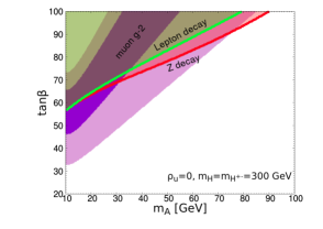
Moreover, any non-zero mixing between and , , does not help explaining the muon in the up-specific VAM because a non-zero always reduces and may turn the originally positive top-loop Barr-Zee contribution negative. Therefore, a large value of is not favored. This is also seen in the charm-specific VAM for the same reason. The parameter region consistent with the muon observation is shown in purple in Fig. 1 for , and .
Lepton universality in decays
The lepton decay processes , and can be used to constrain this model, as they can be mediated at tree level by in addition to the bosons. This is true for any 2HDM’s in general. There are also loop contributions mediated by and 2HDMg2 . The Heavy Flavor Averaging Group (HFAG) gives constraints on the coupling ratios , where hfag . Here we quote the deviations of these ratios from their SM values, : , , and .
By neglecting the electron mass, we obtain , , and , with
| (62) |
where the loop functions , and . Taking correlations among the observables into account, we use the following three independent quantities for the -fit 2HDMg2
| (63) | ||||
Both and are negative in the VAM, while the observed data prefer to have positive values. Thus, we can set an upper bound on for a fixed value of . The 95% CL excluded region is overlaid as the green area in Fig. 1. Note that this constraint is independent of the quark sector and thus the quark mixing parameter .
Lepton universality in decays
The precision measurements at the -pole in both SLD and LEP experiments provide ratios of the leptonic decay branching fractions ALEPH:2005ab . Consider the deviations of such ratios from identity, defined by . Current data have
| (64) |
Corrections due to the loops in the VAM are found to be zdecay
| (65) |
where the SM couplings and . The corrections and from the VAM’s are given by
where , , and the loop functions
| (66) |
The renormalization constant from dimensional regularization will cancel in and .
While the contributions from the VAM’s are negative, the present data exhibit slightly larger values than the SM predictions. Therefore, the large region with an enhancement in the coupling is disfavored. The region excluded at 95% CL is overlaid in the red region in Fig. 1. Note that this constraint is insensitive to the quark sector. From the above considerations, it is seen that small and large are preferred in the up-specific VAM.
Bottom rare decay
In the SM, the flavor-changing neutral current (FCNC) processes are mediated by the loop diagrams with the boson and top quark. In the VAM with non-zero quark mixing angle , the pseudoscalar can couple to the top quark through the coupling. Since is preferred to be light according to the discussions in the previous subsection, its contribution to cannot be neglected. The time-integrated branching ratio averaged between the LHCb bs-LHCb and CMS bs-CMS Collaborations normalized to the SM prediction is reported to be:
| (67) |
The combined SM and VAM contribution to this observable is bs
| (68) |
where and are the decay width difference between the two mass eigenstates and the width of the lighter mass eigenstate, respectively. The pseudoscalar and scalar contributions are given by
| (69) | ||||
where , , and are the Wilson coefficients of the effective four-fermion operators , , and that include contributions from both SM and VAM, with the detailed expressions given in Ref. bs . The measured value of is slightly smaller at the level than the SM prediction out of and .
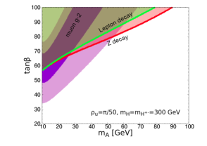
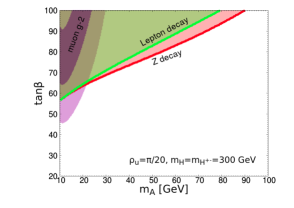
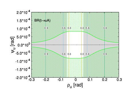
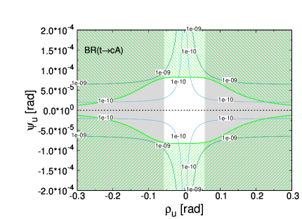
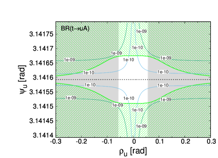
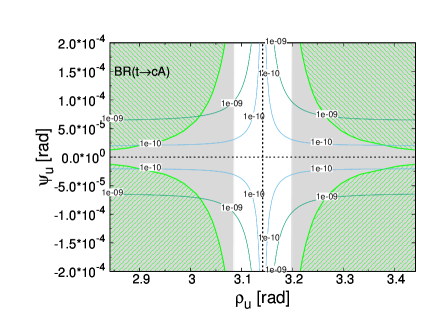
In the up-specific VAM, the main contribution appears in and one can neglect . The contribution from the top- loop diagrams with a pseudoscalar propagator is proportional to . For , the contribution is positive and independent of , with for . As increases, it decreases to zero at and eventually becomes negative. The bottom quark mediated diagrams with a pseudoscalar propagator contribute negatively as for , which is independent of as it is proportional to . In summary, a small but non-zero is preferred to fit the current data, which exhibits a small downward deviation . There exists another solution corresponding to .
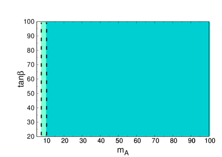
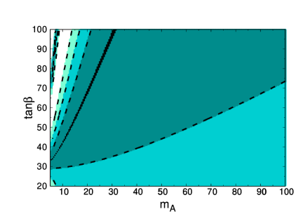
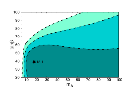
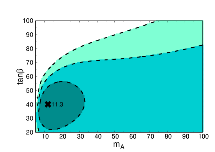
Fig. 2 shows the -contours in the - plane for with (left plot) and (right plot). Shapes of these contours depend sensitively on the value of . Fig. 3 shows the -contours for all the above-mentioned observables taken into account, for (left plot) and (right plot). The best fit point in plane is located around for the whole relevant range of , which is the consistent range to the top total width measurement as we will see in the next section. Such a set of parameters is favored in comparison with the SM () at about 1-2 level. The case would provide a best fit () mainly due to the observed decay branching fraction. In summary so far, the scenario of GeV and with a small mixing angle is preferred by muon without conflicts with the other observables in the up-specific VAM.
oscillation
In the general case when the non-zero flavor violating parameters and are allowed, our model is constrained by more flavor observables. In the following, we examine the flavor violating effects on the meson mixing, the rare top decays, and the total top quark width.
The flavor changing couplings of can contribute to the oscillation at both tree and loop levels. The tree contributions are proportional to and described by the diagrams with the - and -channel exchanges of . The dominant loop-level contributions are proportional to due to and running in the loop. In the VAM, the oscillation imposes the following constraints Harnik:2012pb
| (70) | |||||
| (71) |
The constraints in the - plane for and are shown in Fig. 4, where the hatched green region is excluded at 95% CL. We neglect the interference effects. It is clear that is more constrained than , especially in the up-specific and charm-specific VAM’s. The constraints are weaker in the top-specific case. Even though these plots are drawn by neglecting the flavor-changing contributions from the bosons, there is virtually no change to them even when these diagrams are also included. This is because the mass of are much heavier than in our setup and there is an additional suppression factor of or even though the couplings are proportional to the same factor .
The constraints
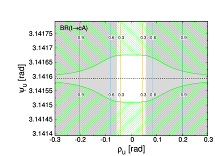
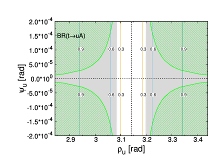
In Fig. 4, we see that is not strongly constrained for by the oscillation data. Currently, one of the most stringent constraints comes from the top FCNS decays of , where and is given by Chiang:2017fjr
| (72) |
The exclusion region generally depends on the value of and , which is empirically found to be close to zero from 125-GeV Higgs coupling measurements. For example, with and , the constraint reads . In the alignment limit , however, these FCNS top decays vanish identically in the up-type VAM.
The constraints from top quark total width
A robust constraint on the FCNS couplings independent of can be obtained from the model-independent top width measurements CMS:2016hdd , where the total top width is reported not to exceed GeV at 95% CL. On the other hand, the VAM’s predict the rare top decays of and . We demand that the total top decay width, including the standard partial width GeV, be below the the upper bound; that is, with
| (73) |
The condition , corresponding to , is translated to for and . Note that it currently provides the most stringent constraint on . The exclusion region is shown by the gray region in Fig. 4.
The decay
When the boson is lighter than , the decay of is kinematically allowed. Although there is a CMS study constraining % Sirunyan:2018pzn , we cannot find the constraint on . Thus, we consider the branching ratio of exotic Higgs decays, which is currently bounded to Curtin:2013fra . Using the partial width formula
| (74) |
we find that the trilinear scalar coupling should satisfy . In the lepton-specific 2HDM with large , can be expressed in terms of neutral Higgs boson masses and lepton Yukawa couplings as Chun:2015hsa
| (75) |
From the first two terms in the numerator, the natural size of is about 60 GeV. Therefore, fine tuning is required for a cancellation between the first two terms and the third term in the numerator, in order to satisfy the experimental constraint on the decay.
Under the constraints of Higgs data: and , we can consider two possible cases. The first case corresponds to the right-sign limit (). However, in the large limit, the bound of GeV is required by the perturbativity condition of the coupling. The charged Higgs mass is then forced to be light due to the condition without conflicting with the electroweak precision measurements. Consequently, the region associated with the right-sign limit is ruled out due to the direct search of the charged Higgs boson at the LHC. The second case corresponds to the wrong-sign limit (), where can be arbitrarily large and, therefore, can be fine-tuned to vanish. The solution for an exact cancellation in in the wrong-sign limit is
| (76) |
for GeV. This is almost independent of provided , as is the case considered here.
Single production at the LHC
In the up-specific VAM, the production at the LHC through the process is enhanced by . For example, for GeV, the production cross section at the 13-TeV LHC reaches
| (77) |
It is, however, too small to detect through the di-muon resonance signal with the current integrated luminosity dimuon .
In this section, we have examined various current constraints on the up-type VAM. As a short summary, we have found that the up-specific VAM with and can provide a good explanation for the deviation found in , while the charm-specific VAM is not favored in this regard. There are no conflict with any flavor observables and experimental measurements considered in this section, as long as the mixing angles and are small. Moreover, taking non-zero at the order of offers a better fit to the branching fraction. This could lead to interesting phenomenology.
IV Smoking gun signatures at LHC
IV.1 Rare top decay
In this section we focus on the up-specific VAM and first consider the most promising signature at the LHC. The analysis shown in this section can be readily applied to the charm-specific case with , although as seen in the previous section this case is slightly disfavored by the observation.
In the VAM with , the decay helicity amplitudes in the limit of are given by
| (78) | ||||
The angle is between the up-quark 3-momentum and the top spin and the up-quark energy in the top rest frame. The direction of up-quark emitted from the top quark is preferentially aligned with the polarization of the top quark. The partial decay width of is easily computed as
| (79) |
which is not suppressed even in the alignment limit, in contrast to the partial decay width that is suppressed by . The branching ratio assuming is, with :
| (80) |
Therefore, for , a of would provide the branching ratio: .
IV.2 Current constraints from existing searches
As top quarks are copiously produced in pairs at the LHC, one should be able to constrain or search for this rare FCNS decay. Nevertheless, we cannot find a dedicated experimental study searching for this specific rare decay in the literature other than several theoretical studies Kao:2011aa ; Chen:2013qta ; Altunkaynak:2015twa . We consider the main production mechanism of the pseudoscalar as , which involves one -jet from the standard top decay. The relevant analyses indirectly constraining this process and at the LHC are the light pseudoscalar Higgs boson searches in association with a pair CMS:2015mca ; Khachatryan:2015baw ; Sirunyan:2017uvf , with several theoretical efforts being made to improve the sensitivity Goncalves:2016qhh ; Banerjee:2017wxi ; Bernon:2014nxa . Among them we find that the CMS analysis at 8 TeV Khachatryan:2015baw currently provides the most stringent constraint. The CMS has shown that the sensitivity using is comparable but weaker than that using , assuming Sirunyan:2017uvf . There are also searches using the di-tau channel on the 13-TeV data Aaboud:2017sjh , although they focus on the case where the new bosons are heavy and only show a limit of GeV at lightest.
We follow the most stringent 8-TeV CMS analysis Khachatryan:2015baw and re-interpret it to constrain our model. For the signal analysis, we use MadGraph5+Pythia8 Alwall:2014hca ; Sjostrand:2007gs for event generation and Delphes3 delphes3 for detector simulation. For jet reconstruction, we rely on the FastJet package Cacciari:2011ma and use the anti-kT algorithm with the standard jet size . The data include three channels: , and , where denotes a tau lepton decaying hadronically, and their respective selection cuts are summarized as follows:
-
•
channel: exactly one and one with opposite charges:
GeV, and GeV, ,
, , -
•
channel: exactly one and one with opposite charges:
GeV, and GeV, ,
, , -
•
channel: exactly one and one with the opposite charge:
( GeV, GeV) or ( GeV, GeV),
and
, , ,
where and is the azimuthal angle difference between the momentum and the missing transverse momentum. The definitions of can be found in Ref. Khachatryan:2015baw . In addition to the above selection cuts, events in all the channels are required to have at least one -tagged jet with and . For the hadronic tagging, we take a simpler algorithm described in Ref. Papaefstathiou:2014oja for the Cambridge/Aachen (C/A) jets with and call a tag when the following conditions are satisfied:
-
•
define by drawing a cone with a smaller radius centered at the jet, and require no tracks with GeV to lie in the annulus between ;
-
•
the hardest track in satisfies GeV; and
-
•
, where , the fraction of jet energy deposited in the jet core.
For the selected events, we consider the possible values of consistent with the kinematics of the two visible tau decay products, and take the minimum value as . We can then set an upper limit on the cross section at 95 % CL. from the combined distribution of all three channels.
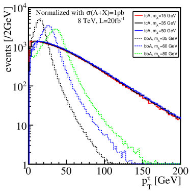
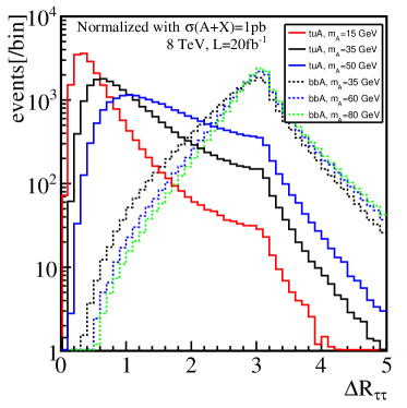
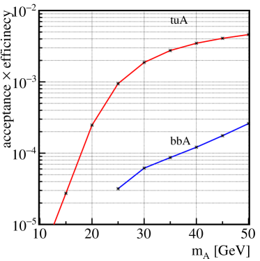
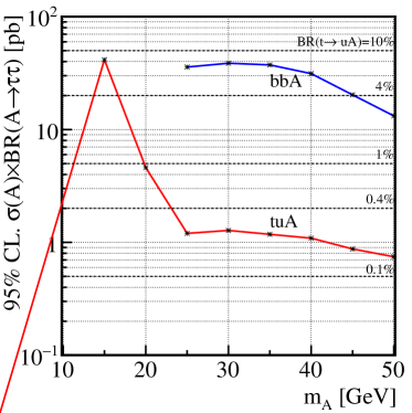
There are two important differences between the decay from production and that from the decay in production (in this section, we shall refer to them as and , respectively). One is that the distribution is softer in the sample when is small, whereas in sample is harder and practically independent of , especially in the tail. This is seen in the upper-left plot of Fig 5, where the normalized distributions in the selected and samples are shown. The other is that the distribution is peaked at in samples whereas it is peaked at for , and more prominent when becomes smaller. The normalized distributions are shown in the upper-right plot of Fig. 5. As a result, the efficiencies of the selection cuts are rapidly falling as gets smaller in both cases of and but for different reasons. The resulting acceptance and efficiency as a function of is shown in the lower-left plot of Fig. 5. As -tagging efficiency rapidly falls as decreases, so is the lepton acceptance from the leptonic tau decay. The final efficiency for the production diminishes when becomes small. On the other hand, the acceptance of the channel is relatively high. For example, it is about 30 times higher than the channel for GeV. Taking this efficiency difference into account, we can re-interpret and apply the constraints obtained for the production to the production. The resulting upper bound on the production cross section at the 95 % CL is shown as a function of in the lower-right plot of Fig. 5. Assuming pb at LHC 8 TeV and is sufficiently small, we can translate the upper bound on the cross section to that on the branching ratio and obtain roughly % for GeV. For GeV, the acceptance is exponentially falling due to the cut. Based on our estimate, % would be allowed for . Since the CMS analysis does not show the results for GeV, we apply in this range the same upper bound on the cross section times the acceptance given at GeV. We consider our results in that range as a conservative estimate because we expect smaller SM background contributions for the appropriate signal region.
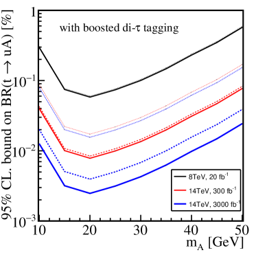
IV.3 Searches using di-tau tagging
In the previous section we have shown that the existing searches become insensitive for the light region, of most interest to us for explaining the muon in our model. In this section we propose an effective way to probe the region, and provide a rough estimate of the expected sensitivity using the current and future data at the LHC.
One of the main reasons for the sensitivity to present a sharp drop in the light region is due to the cut on the reconstructed leptons and taus. For a light , it is boosted from the top decay with the decay products (a di-tau pair from ) being collimated. They are difficult to discriminate and hence naturally captured as one object. We develop the di-tau tagging algorithm following the idea of mutual isolation proposed in the Ref. Katz:2010iq as follows:
-
•
find a jet using the C/A algorithm with ;
-
•
define two exclusive sub-jets and using calorimeter towers in the jet;
-
•
define tau-candidates , by drawing a cone of around each sub-jet;
-
•
for both , require that once the activities (tracks and calorimeters) in are removed, the remaining activity in the original jet satisfy the tau-tagging criteria, with ; and
-
•
the hardest tracks in and are oppositely charged.
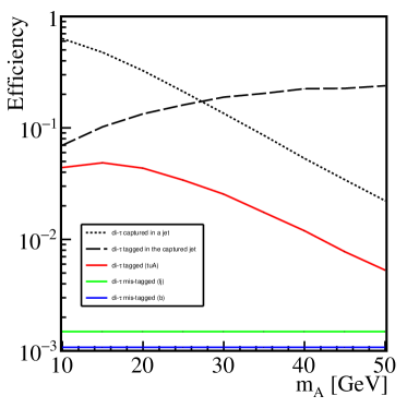
Based on the algorithm described above, the resulting tagging efficiency is shown in the upper left plot of Fig. 6. Note that the tagging efficiency depends on the definition: since the efficiency definition is in general the number of jets tagged divided by the number of preselected jets, there are several possibilities to choose the preselected number as the denominator. First, the efficiency of both visible decay products from the taus in an decay are captured in a jet is shown by the dotted curve as a function of , which rapidly drops as gets larger from 60% to 3%. The tagging efficiency of this algorithm using the number of jets capturing the two visible taus as the denominator is % depending on , as shown by the dashed curve. Finally the overall combined tagging efficiency for the signal ranges from 5% to 0.5% are shown by the red curve, while the mistagging efficiency for the non-tau jets is %. Another analysis quotes a similar di-tau tagging/mis-tag efficiency Conte:2016zjp .
The main background after the appropriate preselection would be , as considered in this paper. A more dedicated analysis would require collaborations with experimental inputs. The set of the preselection is as follows:
-
•
require that the event contains exactly one isolated lepton and at least three jets, with exactly one of them tagged as a -jet and exactly one of them tagged with di-, ;
-
•
GeV and GeV to guarantee that the event contains one standard top decay; and
-
•
to make sure and are from the rare decay, where is the hardest non-, non-di- jet.
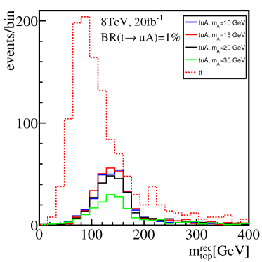
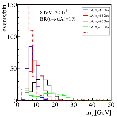
The reconstructed distributions for the signal samples and the background are shown in the upper right plot of Fig. 6. The signal events peak around GeV. Finally, to reduce the remaining background, we make use of the distributions shown in the lower left plot of Fig. 6 and apply the GeV cut. The mass of the signal di- jet has a peak slightly below the corresponding . Based on the remaining number of events after all the selection cuts, we estimate and show the sensitivity to the in the lower right plot of Fig. 6. The resulting current sensitivity would reach below 0.1 % for GeV, which is corresponding to sensitivity on for , and would provide a better sensitivity for GeV compared with the limit given in Fig 5 in the previous section. We also show the future prospects of the sensitivity using 300 fb-1 (3000 fb-1) at 14-TeV LHC. They would reach % for GeV depending on the systematic uncertainty assumption. It will be a factor of improvement from the current constraints. It would be translated to sensitivity on for . The dotted, dashed and solid curves in the plot correspond to the assumed systematic uncertainties of 5 %, 1 %, and 0 %, respectively.
IV.4 Flavor-violating decay of heavy Higgses
Another smoking gun signature of this model is the flavor-violating decays of heavy Higgs bosons and , where we mean flavor-violating decays as those including different generations in the final states.222The SM CKM matrix also initiates such modes, but a more significant fraction of the branching ratio would be expected in the VAM’s with non-zero . Since the characteristic helicity structure is expected, a sizable branching ratio of (including both and for short) and the corresponding should be observed. Existence of these decays would offer a clear difference between the simple type-X 2HDM and the up-specific VAM. Note that when is heavy, though loosing the motivation for explaning , the corresponding flavor-violating decay modes of are also predicted. A modified model with the capacity to accommodate in the heavy scenario will be discussed in the next section.
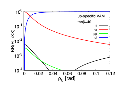
For and , we have
| (81) |
Therefore, the flavor-violating decay dominates for . Fig. 7 shows the branching ratios as a function of for and . For example, reaches 90% for . Since is suppressed due to the new decay mode, the constraint from the searches for the heavy Higgs bosons via the mode could become much weaker in our scenario. It will be even more suppressed with the existence of the other decay modes involving the Higgs bosons, although we assume them negligible here.
Our model also predicts the helicities of top quark in the decay products from the heavy Higgses: the left-handed top or the right-handed anti-top should be observed. Confirming the existence of the decay and measuring the polarization of in the decay products would be an important test for our model.
V Another variants
V.1 Muon-specific in lepton sector
So far, we have assigned the same non-zero PQ charge to charged leptons of all three generations, making their Yukawa couplings to enhanced by . In particular, the enhanced coupling is important to enhance the Barr-Zee diagram contributions to while it is also constrained by the lepton universalities in heavy lepton and decays. Thus, the mass of is required to be lighter than 30 GeV as shown in Fig. 1, which forces us to fine-tune the coupling to zero as decay is always kinematically allowed. For the lepton sector, however, we have more freedom in the PQ charge assignment as they are not relevant to the PQ-solution nor the domain wall problem. From the phenomenological point of view, we can assign a non-zero PQ charge only to and keep and PQ-neutral. We shall refer to the lepton sector in this scenario as the muon-specific lepton sector. It might be even more natural as we have a parallel setup to treat only one generation being special in both lepton and quark sectors. As a result, the and couplings are suppressed by , and the constraints from the heavy lepton and the decays become irrelevant. In this case, the 1-loop contribution dominates over the 2-loop contribution of the suppressed -loop Barr-Zee diagram for Abe:2017jqo . Since among the 1-loop contributions only the one involving the CP-even provides a positive contribution to , as explicitly seen in Table 1, the preferred parameter region has to satisfy . As all the contributions roughly scale like , the required value of to explain the deviation in is about .
In the simple muon-specific model, the LHC data already set lower bounds on and as a plethora of events would be generated through and both and can decay into a pair of muons with a branching ratio of almost 100% due to the enhancement. The search with three or more muons had been performed by the CMS Collaboration using the 13-TeV data with 35.9 fb-1 and found the data consistent with the SM expectation cms-multi , which constrains GeV when we assume Abe:2017jqo . In this case, the decay is kinematically forbidden, and we do not have to worry about the fine-tuning problem of the coupling. With such heavy Higgs masses, would be required to explain the deviation.
With the muon-specific lepton sector, only the up-specific VAM would be valid among the up-type VAM’s as the enhanced 2-loop contributions to are negative for the up-type quarks and only the up Yukawa coupling is small enough to neglect the effects. As the mixing controlled by initiates the enhanced 2-loop -contribution, we cannot consider arbitrary large , as it is not theoretically favored by perturbativity with such a large . We restrict the range of by requiring all Yukawa couplings be perturbative, and obtain from . Within this range, the negative 2-loop top contribution is negligible.
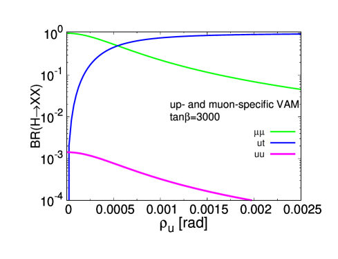
As increases, the enhanced branching ratio of reduces and dominates over the decay of for a good portion of the parameter space. Explicitly, the ratio of their branching ratios is
| (82) |
and ranges from 0 to . In this case, the above-mentioned constraint becomes weaker or invalid for a non-zero . It opens up an allowed region for lighter with the corresponding smaller . Fig. 8 shows the branching fractions as a function of assuming only the fermionic decay modes contribute. Observing the flavor-violating decays would be a smoking gun signature to distinguish between the simple muon-specific 2HDM and the up-type VAM with the muon-specific lepton sector. In this scenario, the flavor-changing rare top decays, and , are kinematically forbidden.
As mentioned above, the charm-specific VAM is difficult to accommodate such large because the 2-loop contribution would dominate over the 1-loop contributions, resulting in an opposite contribution to the . The top-specific VAM is also disfavored by the same reason as the perturbativity of Yukawa couplings. Among the down-type specific VAM’s, down-specific and strange-specific VAM’s would be compatible with the muon-specific lepton sector as the corresponding Yukawa couplings are negligible, analogous to the up-specific case. In the bottom specific VAM, since the enhanced bottom contribution to dominates over the 1-loop contribution, is favored and is required. In this setup, the dominant decay mode of and becomes and the mode is suppressed by , which makes the above-mentioned constraint weaker. However, such an enhancement in the bottom Yukawa coupling would require an extreme fine-tuning at the level of to accommodate the decay branching ratio, since the bottom diagrams contribute as discussed in Sec. III.
V.2 Assigning non-zero PQ charges to down-type RH quarks
Instead of assigning non-zero PQ charge to the RH up-type quarks, we can do the same to the RH down-type quarks without loosing the motivations. In this subsection, we briefly comment on how such a scenario is severely constrained by quark mixing in the down sector. The mixing structure is analogous to the up-type specific VAM, and the mixing matrix would be the same in form as but with and replaced respectively by and to describe the and mixing. We also define in a way analogous to in Eq. (42) with the corresponding substitution. According to Table II of Ref. Harnik:2012pb , the constraints from , and oscillations are:
| (83) | |||||
| (84) | |||||
| (85) |
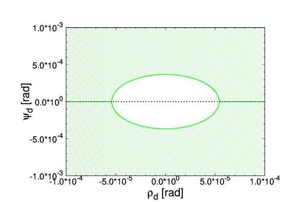
The region in the plane allowed by the above constraints for and is shown by the white region in Fig. 9. Only the region nearby (down-specific VAM) is shown. The constraint is important for , giving . The constraint is important for , giving . The constraint is important for , giving . We define and . There are also allowed regions with (strange-specific VAM) and (bottom-specific VAM). However, as mentioned in the previous section the bottom-specific solution is strongly disfavored by the data.
VI conclusions
We have studied variant axion models (VAM’s) with only a specific fermion charged under the Peccei-Quinn symmetry and their capacity to accommodate the muon anomaly as well as the compatibility with various other experimental constraints. We start by considering the up-type specific VAM’s and find that the combined fit favors the parameters and , the same as the type-X 2HDM. Moreover, we find that this parameter choice has no conflict with flavor observables as long as the mixing angle is sufficiently small. In particular, a small nonzero mixing angle is slightly favored by the observed branching ratio.
As the charm-mediated Barr-Zee diagram contribution to is negative, the charm-specific VAM is disfavored in comparison with the up-specific VAM. We therefore focus on the up-specific model and its promising signature of the rare decay followed by at the LHC. Current searches of already impose some constraints in the parameter space, but do not exclude the most interesting region of . We propose an efficient search strategy that employs di-tau tagging using jet substructure information, and have explicitly demonstrated that it would enhance the sensitivity on , especially in the light region of great interest to us. Our model also predicts that the heavy Higgs bosons have significant flavor-violating decays, such as . We encourage our experimental colleagues to search intensively for this flavor-changing top decay and the flavor-violating resonances.
We have also considered other variants: the muon-specific lepton sector and the down-type specific VAM’s. The up-specific VAM with the muon-specific lepton sector is very interesting possibility as no tuning is required to suppress and the scenario is not constrained by the lepton universality measurements. Unlike the simplest muon-specific model, the up-specific VAM with the muon-specific sector predicts that the heavy Higgs bosons can decay into a pair of flavor-violating up-type quarks such as at a significant branching fraction. It suppresses the decay, making the constraint at the LHC less effective and opens up more parameter space. The down/strange-specific VAM’s with the muon-specific lepton sector would also be viable possibilities. The down-type specific VAM’s are strongly constrained by the decay and the and meson mixing data, rendering a very fine-tuned parameter space. Nevertheless, such scenarios could offer another interesting possibility to explain as one of the bottom Barr-Zee diagram contribution is positive.
Acknowledgments
The authors would like to thank Kei Yagyu for some discussions about the -specific lepton sector. This research was supported in part by the Ministry of Science and Technology of Taiwan under Grant No. NSC 100-2628-M-008-003-MY4 (C.-W. C); the Japan Society for the Promotion of Science (JSPS) Grant-in-Aid for Scientific Research Numbers No. 26104001, No. 26104009, No. 16H02176, and No. 17H02878 (T. T. Y.); and the World Premier International Research Center Initiative, MEXT, Japan (M. T., P.-Y. T, and T. T. Y.). MT is supported in part by the JSPS Grant-in-Aid for Scientific Research Numbers 16H03991, 16H02176, 17H05399, and 18K03611.
References
- (1) R. D. Peccei and H. R. Quinn, Phys. Rev. Lett. 38, 1440 (1977).
- (2) S. Weinberg, Phys. Rev. Lett. 40, 223 (1978).
- (3) F. Wilczek, Phys. Rev. Lett. 40, 279 (1978).
- (4) K. A. Olive et al. [Particle Data Group Collaboration], Chin. Phys. C 38, 090001 (2014).
- (5) L. F. Abbott and P. Sikivie, Phys. Lett. B 120, 133 (1983).
- (6) J. Preskill, M. B. Wise and F. Wilczek, Phys. Lett. B 120, 127 (1983).
- (7) M. Dine and W. Fischler, Phys. Lett. B 120, 137 (1983).
- (8) P. A. R. Ade et al. [Planck Collaboration], arXiv:1502.01589 [astro-ph.CO].
- (9) R. D. Peccei, T. T. Wu and T. Yanagida, Phys. Lett. B 172, 435 (1986).
- (10) L. M. Krauss and F. Wilczek, Phys. Lett. B 173, 189 (1986).
- (11) C. R. Chen, P. H. Frampton, F. Takahashi and T. T. Yanagida, JHEP 1006, 059 (2010) [arXiv:1005.1185 [hep-ph]].
- (12) C. W. Chiang, H. Fukuda, M. Takeuchi and T. T. Yanagida, JHEP 1511, 057 (2015) [arXiv:1507.04354 [hep-ph]].
- (13) C. W. Chiang, H. Fukuda, M. Takeuchi and T. T. Yanagida, Phys. Rev. D 97, no. 3, 035015 (2018) [arXiv:1711.02993 [hep-ph]].
- (14) K. Hagiwara, R. Liao, A. D. Martin, D. Nomura and T. Teubner, J. Phys. G 38, 085003 (2011) [arXiv:1105.3149 [hep-ph]].
- (15) E. J. Chun, EPJ Web Conf. 118, 01006 (2016) [Pramana 87, no. 3, 41 (2016)] [arXiv:1511.05225 [hep-ph]].
- (16) E. J. Chun, Z. Kang, M. Takeuchi and Y. L. S. Tsai, JHEP 1511, 099 (2015), [arXiv:1507.08067 [hep-ph]].
- (17) T. Abe, R. Sato and K. Yagyu, JHEP 1707, 012 (2017), [arXiv:1705.01469 [hep-ph]].
- (18) G. W. Bennett et al. [Muon g-2 Collaboration], Phys. Rev. D 73, 072003 (2006), [hep-ex/0602035].
- (19) F. Jegerlehner and A. Nyffeler, Phys. Rept. 477, 1 (2009), [arXiv:0902.3360 [hep-ph]].
- (20) A. Broggio, E. J. Chun, M. Passera, K. M. Patel and S. K. Vempati, JHEP 1411, 058 (2014), [arXiv:1409.3199 [hep-ph]].
- (21) Y. Amhis et al. [Heavy Flavor Averaging Group (HFAG)], [arXiv:1412.7515 [hep-ex]].
- (22) S. Schael et al. [ALEPH and DELPHI and L3 and OPAL and SLD Collaborations and LEP Electroweak Working Group and SLD Electroweak Group and SLD Heavy Flavour Group], Phys. Rept. 427, 257 (2006), [hep-ex/0509008].
- (23) E. J. Chun and J. Kim, JHEP 1607, 110 (2016), [arXiv:1605.06298 [hep-ph]].
- (24) R. Aaij et al. [LHCb Collaboration], Phys. Rev. Lett. 111, 101805 (2013), [arXiv:1307.5024 [hep-ex]].
- (25) S. Chatrchyan et al. [CMS Collaboration], Phys. Rev. Lett. 111, 101804 (2013), [arXiv:1307.5025 [hep-ex]].
- (26) X. Q. Li, J. Lu and A. Pich, JHEP 1406, 022 (2014), [arXiv:1404.5865 [hep-ph]].
- (27) R. Harnik, J. Kopp and J. Zupan, JHEP 1303, 026 (2013), [arXiv:1209.1397 [hep-ph]].
- (28) CMS Collaboration [CMS Collaboration], CMS-PAS-TOP-16-019.
- (29) A. M. Sirunyan et al. [CMS Collaboration], arXiv:1805.10191 [hep-ex].
- (30) D. Curtin et al., Phys. Rev. D 90, no. 7, 075004 (2014), [arXiv:1312.4992 [hep-ph]].
- (31) I. Hoenig, G. Samach and D. Tucker-Smith, Phys. Rev. D 90, no. 7, 075016 (2014), [arXiv:1408.1075 [hep-ph]].
- (32) C. Kao, H. Y. Cheng, W. S. Hou and J. Sayre, Phys. Lett. B 716, 225 (2012) [arXiv:1112.1707 [hep-ph]].
- (33) K. F. Chen, W. S. Hou, C. Kao and M. Kohda, Phys. Lett. B 725, 378 (2013) [arXiv:1304.8037 [hep-ph]].
- (34) B. Altunkaynak, W. S. Hou, C. Kao, M. Kohda and B. McCoy, Phys. Lett. B 751, 135 (2015) [arXiv:1506.00651 [hep-ph]].
- (35) CMS Collaboration [CMS Collaboration], CMS-PAS-HIG-14-029.
- (36) V. Khachatryan et al. [CMS Collaboration], Phys. Lett. B 758, 296 (2016) [arXiv:1511.03610 [hep-ex]].
- (37) A. M. Sirunyan et al. [CMS Collaboration], JHEP 1711, 010 (2017) [arXiv:1707.07283 [hep-ex]].
- (38) D. Goncalves and D. Lopez-Val, Phys. Rev. D 94, no. 9, 095005 (2016) [arXiv:1607.08614 [hep-ph]].
- (39) S. Banerjee, D. Barducci, G. Belanger, B. Fuks, A. Goudelis and B. Zaldivar, JHEP 1707, 080 (2017) [arXiv:1705.02327 [hep-ph]].
- (40) J. Bernon, J. F. Gunion, Y. Jiang and S. Kraml, Phys. Rev. D 91, no. 7, 075019 (2015) [arXiv:1412.3385 [hep-ph]].
- (41) M. Aaboud et al. [ATLAS Collaboration], JHEP 1801, 055 (2018) [arXiv:1709.07242 [hep-ex]].
- (42) J. Alwall et al., JHEP 1407, 079 (2014) [arXiv:1405.0301 [hep-ph]].
- (43) T. Sjostrand, S. Mrenna and P. Z. Skands, Comput. Phys. Commun. 178, 852 (2008) [arXiv:0710.3820 [hep-ph]].
- (44) J. de Favereau et al. [DELPHES 3 Collaboration], JHEP 1402, 057 (2014)
- (45) M. Cacciari, G. P. Salam and G. Soyez, Eur. Phys. J. C 72, 1896 (2012) [arXiv:1111.6097 [hep-ph]].
- (46) A. Papaefstathiou, K. Sakurai and M. Takeuchi, JHEP 1408, 176 (2014) [arXiv:1404.1077 [hep-ph]].
- (47) A. Katz, M. Son and B. Tweedie, Phys. Rev. D 83, 114033 (2011) [arXiv:1011.4523 [hep-ph]].
- (48) E. Conte, B. Fuks, J. Guo, J. Li and A. G. Williams, JHEP 1605, 100 (2016) [arXiv:1604.05394 [hep-ph]].
- (49) CMS Collaboration [CMS Collaboration], CMS-PAS-EXO-17-006, [arXiv:1708.07962 [hep-ex]].