Light Dark Matter Showering under Broken Dark $U(1)$ – Revisited

Abstract

It was proposed recently that different chiralities of the dark matter (DM) fermion under a broken dark U(1) gauge group can lead to distinguishable signatures at the LHC through shower patterns, which may reveal the mass origin of the dark sector. We study this subject further by examining the dark shower of two simplified models, the dubbed Chiral Model and the Vector Model. We derive a more complete set of collinear splitting functions with power corrections, specifying the helicities of the initial DM fermion and including the contribution from an extra degree of freedom, the dark Higgs boson. The dark shower is then implemented with these splitting functions, and the new features resulting from its correct modelling are emphasized. It is shown that the DM fermion chirality can be differentiated by measuring dark shower patterns, especially the DM jet energy profile, which is almost independent of the DM energy.

I Introduction

The nature of dark matter (DM) remains one of the most challenging puzzles in modern physics. One of the popular scenarios is that the DM is composed of weakly interacting massive particles (WIMP) Lee:1977ua , as strongly motivated by the supersymmetric framework Jungman:1995df . Null results of direct detection and LHC search have highly constrained this scenario in recent years. Meanwhile, new evidences such as the positron excess in cosmic ray spectra Adriani:2008zr , the tension between the cold DM model and the small structure observations of the universe Spergel:1999mh , etc. have led us to consider other options. One possibility is that there exists a new interaction in the dark sector ArkaniHamed:2008qp ; Alexander:2016aln ; ArkaniHamed:2008qn ; Cirelli:2008pk , given the rich dynamical structure in the Standard Model (SM). In particular, stability or longevity of DM particles could be associated with exact or approximate quantum numbers, that might be in turn the results of exact gauge symmetries or accidental symmetries of underlying dark gauge groups, in analogy with the electron stability and the proton longevity (see Refs. Baek:2013qwa ; KO:2016gxk for discussions along this line of thoughts).

The simplest candidate for the new dark gauge interaction arises from a hidden $U(1)$ gauge group which is kinetically mixed with the $U(1)$ sector in the SM. The study of a new $U(1)$ gauge group has a long history Holdom:1985ag . The operation of the LHC has provided a unique opportunity to test various scenarios with new $U(1)$ interactions Cohen:2017pzm . Here we are interested in a light DM charged under a dark $U(1)_{d}$ group with the mass around the sub-GeV scale. As this light DM is produced energetically at a collider, it radiates multiple collimated $U(1)_{d}$ gauge bosons, i.e., dark photons, which then decay back into SM particles, forming detectable leptonic or hadronic jets. This is an analogue to the phenomenon called the parton shower in the SM, especially the electroweak (EW) shower Chen:2016wkt , if the dark photon has a small mass. The subject on the dark shower has been investigated recently in the literature: both analytical and Monte Carlo methods were applied to the model, in which DM fermions interact with gauge fields only through a vector current Buschmann:2015awa ; both the vector and the axial vector interactions were considered in Zhang:2016sll , where it was pointed out that whether left-handed and right-handed fermions have different interactions with gauge bosons could be determined by measuring the dark shower patterns at the LHC.

In this paper we will further explore the relation between the dark shower patterns and the chirality of the DM fermion, motivated by the close connection of the DM property under the gauge group to the mass origin in the dark sector. The dark photon mass can come from two types of mechanism, the Higgs mechanism and the Stüeckelberg mechanism Bell:2016uhg ; Ruegg:2003ps . The latter can be seen as a limiting case of the former with the Higgs sector – including the longitudinal gauge boson after symmetry breaking and the Higgs boson – decoupling from a theory, such that the fermion involved in the former (the latter) prefers to be chiral-like (vector-like). The dark shower pattern is then mainly governed by transversely polarized dark photons in the case of the Stüeckelberg mechanism, but receives additional contributions from longitudinally polarized dark photons and dark Higgs bosons in the case of the Higgs mechanism. Because transversely polarized dark photons tend to be soft, while longitudinally polarized dark photons and dark Higgs bosons do not, different shower patterns can be produced in the two scenarios. Therefore, exploring the chiral behavior of the DM fermion through the dark shower patterns helps understand the origin of the dark photon mass.

The rest of the paper is organized as follows. In Sec. II, we elaborate the two mass generation mechanisms for dark photons and how they are related to the chiral property of the DM fermion. Two simplified models, the Chiral Model and the Vector Model, are introduced for the realization of mass generation. In Sec. III, we explain the setting of the dark shower and the role of the splitting functions, mentioning some subtleties attributed to particle mass effects. The splitting functions with the DM fermions as the initial particles in the considered models are then derived according to the formalism for the EW shower in Ref. Chen:2016wkt . In Sec. IV, we implement the dark shower with the Monte Carlo program developed in Ref. Chen:2016wkt , examine several observables associated with the dark shower, and highlight the different patterns between the two models. It will be demonstrated that the DM jet energy profile, being almost independent of the DM energy, is an appropriate observable for differentiating the DM fermion chirality. We intend to explore the properties of new dark $U(1)$ gauge boson showers possibly produced at LHC as an application of the results in Chen:2016wkt , and to lay out a correct framework for studying this topic. We emphasize that there has not been a complete treatment of the dark splitting functions and the dark shower implementation in the literature. Section V is the conclusion. Some examples on the calculation of the splitting functions are presented in the Appendix.

II Models

A peculiar observation about an abelian gauge theory is that a gauge boson can obtain a mass without the Higgs mechanism, while the theory still remains gauge invariant and renormalizable. The mechanism is referred to as the Stüeckelberg mechanism Bell:2016uhg ; Ruegg:2003ps which differs from the well-known Higgs mechanism in the number of degrees of freedom. The latter requires an additional scalar field charged under the gauge group to induce symmetry breaking, after which the Goldstone modes are “eaten” by the gauge fields to become the longitudinal polarizations. As the dark photon mass is generated through the Higgs mechanism, there are effectively two more degrees of freedom, the longitudinal polarization of the dark photon and the dark Higgs boson. The Stüeckelberg mechanism is a limiting case of the Higgs mechanism, in which the vacuum expectation value (VEV) of the Higgs boson approaches to infinity, while the Higgs charge and the Yukawa coupling approach to zero in the way that the gauge boson (fermion) mass, proportional to the product of the Higgs charge (Yukawa coupling) and the VEV, remains fixed. The Higgs boson, with its mass being proportional to the product of the square root of the finite Higgs self-coupling and the VEV, then decouples. Hence, if the dark photon obtains its mass through the Stüeckelberg mechanism, neither the Goldstone mode nor the dark Higgs boson will exist.

As stated in the introduction, the origin of the dark photon mass is closely related to the DM fermion property under the gauge group $U(1)_{d}$. The argument goes as follows: we first assume that the DM fermion is of the Dirac type and has some generic interactions with the dark photon. If the DM fermion is chiral-like, the left-handed fermion and the right-handed fermion can have different $U(1)_{d}$ charges, and a bare mass term for the fermion is forbidden by the $U(1)_{d}$ symmetry. Similarly to the SM, a dark Higgs field has to be introduced to give the fermion mass, which then gives the dark photon mass as well naturally. Thus the dark photon mass is likely to be induced by the Higgs mechanism in this case. Alternatively, if the DM fermion is vector-like, the left-handed and right-handed fermions have the same charge under the dark $U(1)_{d}$ group. It is then impossible for the fermion mass to come from the symmetry breaking of a Higgs sector under the same $U(1)_{d}$ group. It is also natural to assume that the dark photon mass is attributed to the Stüeckelberg mechanism without a Higgs sector.

We realize the above two scenarios with the simplified models below. The Chiral Model for the implementation of the Higgs mechanism is defined as

$${\cal L} = -\frac{1}{4}F^{\prime}_{\mu\nu}F^{\prime\mu\nu}+\frac{\epsilon}{2}F^{\prime}_{\mu\nu}F^{\mu\nu}+|D_{\mu}\Phi^{\prime}|^{2}-\frac{\lambda_{\Phi^{\prime}}}{4}\left(|\Phi^{\prime}|^{2}-\frac{v_{\Phi^{\prime}}^{2}}{2}\right)^{2}$$ (1)

$$+\sum_{s=L/R}i\overline{\chi}_{s}\not{D}\chi_{s}-\left(y_{\chi}\overline{\chi_{L}}\Phi^{\prime}\chi_{R}+h.c.\right),$$

where the fields with primes represent the dark fields, $\epsilon$ describes the mixing strength between the dark and SM photons, $D_{\mu}=\partial_{\mu}-ig^{\prime}Q_{s}A^{\prime}_{\mu}$ with $s=L/R$ for the left-/right-handed DM fermion $\chi_{s}$, the Higgs charge $Q_{\Phi^{\prime}}$ appearing in $D_{\mu}\Phi^{\prime}$ is given by $Q_{\Phi^{\prime}}=Q_{L}-Q_{R}$, and $\lambda_{\Phi^{\prime}}$ and $y_{\chi}$ denote the dark Higgs self-coupling and the dark Yukawa coupling, respectively. The scalar field can be parameterized as $\Phi^{\prime}=\frac{1}{\sqrt{2}}(h^{\prime}+i\phi^{\prime})$. After dark gauge symmetry breaking, $\Phi^{\prime}$ acquires a VEV $v_{\Phi^{\prime}}$ along the direction of $h^{\prime}$: $h^{\prime}\rightarrow h^{\prime}+v_{\Phi^{\prime}}$, and particles get their masses with the dark photon mass $m_{A^{\prime}}=g^{\prime}Q_{\Phi^{\prime}}v_{\Phi^{\prime}}$, the dark fermion mass $m_{\chi}=\frac{y_{\chi}v_{\Phi^{\prime}}}{\sqrt{2}}$, and the dark Higgs mass $m_{h^{\prime}}^{2}=\frac{\lambda_{\Phi^{\prime}}v_{\Phi^{\prime}}^{2}}{2}$. Here we have adopted the sign convention of the coupling, so that $g^{\prime}Q_{\Phi^{\prime}}>0$ and $y_{\chi}>0$.

It is easy to see that Eq. (1) reduces to the Vector Model for the Stüeckelberg mechanism in the limits $v_{\Phi^{\prime}}\to\infty$, $Q_{\Phi^{\prime}}\to 0$, and $y_{\chi}\to 0$ with finite $m_{A^{\prime}}$ and $m_{\chi}$,

$${\cal L}=-\frac{1}{4}F^{\prime}_{\mu\nu}F^{\prime\mu\nu}+\frac{\epsilon}{2}F^{\prime}_{\mu\nu}F^{\mu\nu}+\frac{1}{2}m_{A^{\prime}}^{2}A^{\prime}_{\mu}A^{\prime\mu}+\sum_{s}\overline{\chi}_{s}\left(i\not{D}-m_{\chi}\right)\chi_{s},$$ (2)

for which we have $Q_{L}=Q_{R}$.

The two models are typical, and do not cover all the possibilities Bell:2016uhg . In the chiral case, other possibilities are highly constrained by the unitarity and gauge invariance Kahlhoefer:2015bea , such that a dark Higgs sector seems to be inevitable. In the vector case, the dark photon mass is still allowed to arise from the Higgs mechanism, but we would need to add additional degrees of freedom to the model. Because these possibilities do not modify the relation between the shower patterns and the DM fermion chirality essentially, we will ignore them here without losing generality, and leave them to future works.

III Collinear Splitting functions and Dark Shower

III.1 Mass Effects

When the masses of the DM and the dark photon are much lower than the center-of-mass energy of a collider, their production rates are greatly enhanced in collinear regions of radiative corrections, leading to multiple dark particles collimated with the DM along a certain direction. This dark shower is in analogy to the QCD and EW showers in the SM. If the dark photon has a finite mixing with the SM photon, the produced dark photons may decay into SM particles, resulting in signatures of lepton jets Buschmann:2015awa or light-hadron jets.

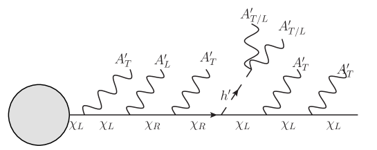
Figure 1: Illustration of dark shower in the Chiral Model.

The evolution of the dark shower initiated by the mother particle $A$ through the radiation $A\rightarrow B+C$ is controlled by the Sudakov form factor

$$\Delta_{A}(t)=\text{exp}\left[-\sum_{B,C}\int_{t_{0}}^{t}dt^{\prime}\int dz\frac{d{\mathcal{P}}_{A\rightarrow B+C}}{dzdt^{\prime}}\right],$$ (3)

which sums all possible collinear splitting functions $\frac{d{\mathcal{P}}_{A\rightarrow B+C}}{dzdt^{\prime}}$. The variable $z=\frac{E_{C}}{E_{A}}$ is the energy fraction of the particle $C$ to the particle $A$. The evolution variable is usually taken as $t=\log(k_{T}^{2})$ or $t=\log(q^{2})$ with $k_{T}$ being the transverse momentum of a final state particle and $q^{2}$ being the virtuality of $A$. The lower bound $t_{0}=\log(m_{\text{cutoff}}^{2})$ corresponds to the infrared cutoff scale $m_{\text{cutoff}}={\rm max}(m_{A^{\prime}},m_{\chi},m_{h^{\prime}})$. As seen below, the mass terms in the splitting functions play the role of an infrared cutoff, so that the choice of $t_{0}$ is largely irrelevant as long as it is not higher than the mass scale of the theory.

The dark shower in a massive $U(1)$ theory bears many similarities to the EW shower. In Ref. Chen:2016wkt , all the $1\rightarrow 2$ EW splitting functions were derived, including the broken splitting functions that are proportional to the VEV of the Higgs field, or equivalently, particle masses. The splitting function $\frac{d{\mathcal{P}}_{A\rightarrow B+C}}{dzdk_{T}^{2}}$ can be expanded in powers of $\frac{m^{2}}{k_{T}^{2}}$ Chen:2016wkt in a model with symmetry breaking,

$$\text{leading power}:\ \ \ \frac{d{\mathcal{P}}_{A\rightarrow B+C}}{dzdk_{T}^{2}} \propto \frac{k_{T}^{2}}{\tilde{k}_{T}^{4}},$$ (4)

$$\text{next-to-leading power: }\ \ \ \frac{d{\mathcal{P}}_{A\rightarrow B+C}}{dzdk_{T}^{2}} \propto \frac{m^{2}}{\tilde{k}_{T}^{4}},$$ (5)

where the mass parameter $m$ depends on the specific splitting process. The denominator $\tilde{k}_{T}^{4}=(\tilde{k}_{T}^{2})^{2}$ is written in terms of

$$\tilde{k}_{T}^{2}=k_{T}^{2}+\bar{z}m_{B}^{2}+zm_{C}^{2}-z\bar{z}m_{A}^{2},$$ (6)

with $\bar{z}=1-z$. The splitting functions at the leading power, being mass independent, correspond to those in the unbroken theory. The splitting functions from the next-to-leading-power corrections are more enhanced at low $k_{T}$ relative to the unbroken splittings, and called the “ultra-collinear” splittings Chen:2016wkt . The origin of the ultra-collinear splittings can be interpreted as the VEV insertions into either particle propagators or splitting vertices Chen:2016wkt .

Compared to the splitting functions for massless particles, we have replaced $\frac{1}{k_{T}^{2}}$ by $\frac{k_{T}^{2}}{\tilde{k}_{T}^{4}}$ effectively, such that the mass terms in $\tilde{k}_{T}^{4}$ play the role of an infrared regulator. The evolution of the parton shower will shut off automatically, when it approaches to the infrared scale. Note that the infrared regularization in the QCD shower is implemented with a sharp cutoff, below which the hadronization takes place. The mass effects are included in Pythia Sjostrand:2014zea currently by adding an extra term to the splitting function Buschmann:2015awa ,

$$\frac{1}{k_{T}^{2}}\rightarrow\frac{1}{k_{T}^{2}}+\frac{m^{2}}{k_{T}^{4}},$$ (7)

equivalent to the Taylor expansion of $\frac{k_{T}^{2}}{\tilde{k}_{T}^{4}}$ around $\frac{1}{k_{T}^{2}}$ to the order of $\frac{m^{2}}{k_{T}^{2}}$.

The separation of the unbroken and broken pieces is best illustrated in the splittings containing longitudinal vector bosons. Naively, the splitting function for $\chi\rightarrow\chi A^{\prime}_{L}$ can be obtained through the Goldstone equivalence theorem, whose contribution, however, accounts only for the unbroken piece. It has been proposed to take into account the symmetry breaking effects by imposing the Goldstone equivalence gauge (GEG) Chen:2016wkt . To explain what this new gauge does, we write the longitudinal polarization vector as

$$\epsilon^{\mu}_{L}=\frac{k^{\mu}}{m_{A^{\prime}}}-\frac{m_{A^{\prime}}}{n\cdot k}n^{\mu},$$ (8)

with the momentum of the vector boson $k^{\mu}=(k^{0},\vec{k})$ and the direction of GEG being defined by a null vector $n^{\mu}=(1,-\hat{k})$ with $\hat{k}\cdot\hat{k}=1$. The term $\frac{k^{\mu}}{m_{A^{\prime}}}$ is the one that gives rise to the aforementioned contribution of the Goldstone equivalence. It induces a bad high-energy behavior and large interference among diagrams, complicating many calculations, such as those of the collinear splitting functions. Working in the GEG along $n^{\mu}$ renders this term, which violates the gauge condition because of $n\cdot k\neq 0$, not contribute to physical polarizations. Instead, it manifests itself as a Goldstone mode. The remnant term $-\frac{m_{A^{\prime}}}{n\cdot k}n^{\mu}$ survives, since $n\cdot n=0$, namely, the gauge condition is satisfied. The amplitudes involving longitudinal vector bosons are then evaluated by summing diagrams for both the Goldstone and gauge components in GEG. These two components bear different physical significance to the splitting functions: the former, that flips the fermion helicity, contributes to splittings at leading power of $\frac{m^{2}}{k_{T}^{2}}$; while the latter, that does not flip the fermion helicity, contributes at next-to-leading power, i.e., to the ultra-collinear splittings as seen in the next subsection. Besides, the fermion mass also contributes to the ultra-collinear splittings in a similar way.

III.2 Splitting Functions

The splitting functions in the Chiral Model and Vector Model are described by the same set of parameters $\alpha^{\prime}=g^{\prime 2}/(4\pi)$, $m_{A^{\prime}}$, $m_{\chi}$, $m_{h^{\prime}}$, as well as $Q_{L}$ and $Q_{R}$, in terms of which all other parameters $Q_{\Phi^{\prime}}$, $y_{\chi}$, and $\lambda_{\Phi^{\prime}}$ can be expressed. We focus on the splittings with $\chi$ being the only initial state in the present work. The leading power splittings are given by

$$\frac{d{\mathcal{P}}}{dzdk_{T}^{2}}(\chi_{s}\rightarrow\chi_{s}+A^{\prime}_{T}) = \frac{\alpha^{\prime}}{2\pi}Q_{s}^{2}\frac{1+\bar{z}^{2}}{z}\frac{k_{T}^{2}}{\tilde{k}_{T}^{4}},$$ (9)

$$\frac{d{\mathcal{P}}}{dzdk_{T}^{2}}(\chi_{s}\rightarrow\chi_{-s}+A^{\prime}_{L}) = \frac{\alpha^{\prime}}{2\pi}\frac{m_{\chi}^{2}}{m_{A^{\prime}}^{2}}Q_{\Phi^{\prime}}^{2}\frac{z}{2}\frac{k_{T}^{2}}{\tilde{k}_{T}^{4}},$$ (10)

$$\frac{d{\mathcal{P}}}{dzdk_{T}^{2}}(\chi_{s}\rightarrow\chi_{-s}+h^{\prime}) = \frac{\alpha^{\prime}}{2\pi}\frac{m_{\chi}^{2}}{m_{A^{\prime}}^{2}}Q_{\Phi^{\prime}}^{2}\frac{z}{2}\frac{k_{T}^{2}}{\tilde{k}_{T}^{4}},$$ (11)

where $s$ denotes both the helicity $\pm 1/2$ in $\chi_{s}$ and the chirality $L/R$ in $Q_{s}$. The helicity and the chirality become identical in the high energy limit with $s=\mp\frac{1}{2}$ corresponding to $s=L/R$ for particles (as opposed to antiparticles). Here we use left-handed/right-handed to label the helicity and the chirality interchangeably. It is found from the above splitting functions that the radiation of transversely polarized dark photons exhibits a soft enhancement at small $z$, and that the radiations of longitudinally polarized dark photons and dark Higgs bosons diminish at leading power in the Vector Model due to $Q_{\Phi^{\prime}}=0$. These are the major features which cause the different dark shower pattens in the Chiral and Vector Models.

We have the next-to-leading-power splitting functions

$$\frac{d{\mathcal{P}}}{dzdk_{T}^{2}}(\chi_{s}\rightarrow\chi_{-s}+A^{\prime}_{T}) = \frac{\alpha^{\prime}}{2\pi}z(Q_{s}-Q_{-s}\bar{z})^{2}\frac{m_{\chi}^{2}}{\tilde{k}_{T}^{4}},$$ (12)

$$\frac{d{\mathcal{P}}}{dzdk_{T}^{2}}(\chi_{s}\rightarrow\chi_{s}+A^{\prime}_{L}) = \frac{\alpha^{\prime}}{2\pi}\frac{1}{2z}\left(2Q_{s}\bar{z}+(-1)^{s+\frac{1}{2}}\frac{z^{2}m_{\chi}^{2}}{m_{A^{\prime}}^{2}}Q_{\Phi^{\prime}}\right)^{2}\frac{m_{A^{\prime}}^{2}}{\tilde{k}_{T}^{4}},$$ (13)

$$\frac{d{\mathcal{P}}}{dzdk_{T}^{2}}(\chi_{s}\rightarrow\chi_{s}+h^{\prime}) = \frac{\alpha^{\prime}}{2\pi}Q_{\Phi^{\prime}}^{2}\frac{z(1+\bar{z})^{2}}{2}\frac{m_{\chi}^{2}}{m_{A^{\prime}}^{2}}\frac{m_{\chi}^{2}}{\tilde{k}_{T}^{4}}.$$ (14)

At this subleading level, longitudinally polarized dark photons contribute in the Vector Model, but dark Higgs boson still do not. As shown in the next section, the next-to-leading-power effects on the dark shower patterns are less important.

In the above derivation with only the dark radiation, we have assumed that the mass eigenstate of the massive dark photon is what appears in the Lagrangian. Strictly speaking, we need to perform the field redefinition and diagonalize the mass matrix to find the real mass eigenstates first. After the diagonalization, the real massless eigenstate does not interact with the DM fermion directly, and the massive dark photon can be also radiated by a SM fermion, such as a colliding parton, whose effect is, however, suppressed by the mixing parameter $\epsilon$. Besides, the $1\rightarrow 2$ splitting amplitudes mainly collect collinear contributions, and it has been known that different collinear sub-processes do not affect each other significantly. Including a $U(1)_{Y}$ gauge group from the SM side, we get an additional interaction between the DM fermion and the $Z$ boson. This interaction does not induce new collinear splittings, because the $Z$ boson mass is much larger than the mass scale considered here.

Compared with Ref. Zhang:2016sll and the setting in Pythia, our formulae have several important differences:

• In the splittings, we treat the fermion helicities separately. This is necessary, because it is not guaranteed that the initial particle in the shower is unpolarized. Moreover, the fermion flips its helicity in some splittings, leading to nontrivial interplay between different helicities, which cannot be captured by naively taking an average of the initial helicities in the splittings. Especially, we find that even though the DM is unpolarized initially, it can obtain a certain polarization after showering in our setup.

• We incorporate the dark Higgs boson contribution in the splitting functions, since it arises naturally along with the Goldstone mode in the Chiral Model.

• Our splitting function for $\chi_{s}\rightarrow\chi_{-s}+A^{\prime}_{L}$ contains an additional factor $z/2$ relative to the result in Ref. Zhang:2016sll , which arises from the choice of the wave function for the initial state fermion in the evaluation of the splitting functions. We point out that in order for proper factorization of the collinear splitting functions from hard processes, the “on-shell” wave function is required regardless of the kinematics, as elaborated further in Appendix A.

• We have one more set of splitting functions (scaling as $\frac{m^{2}}{k_{T}^{4}}$) attributed to the symmetry breaking, which are more enhanced in the small $k_{T}$ region than the leading-power splitting functions.

IV Implementation of Dark Showering

We implement the dark shower with the derived splitting functions using the EW shower program from Ref. Chen:2016wkt , and compare its patterns in the Chiral Model and Vector Model at several benchmark points. For the same couplings and masses, the difference between the two models is characterized by the charge ratio $Q_{L}/Q_{R}$. Following Ref. Zhang:2016sll for an immediate comparison, we choose $(Q_{V},Q_{A})=(1,1)$ for the Chiral Model and $(Q_{V},Q_{A})=(1,0)$ for the Vector Model, where $Q_{V}=\frac{Q_{L}+Q_{R}}{2}$ and $Q_{A}=\frac{Q_{L}-Q_{R}}{2}$. Except for the dark Higgs mass $m_{h^{\prime}}$, the other parameters of the models are also the same as in Ref. Zhang:2016sll . Three benchmark points A, B and C are selected as

point A: $$\alpha^{\prime}=0.3\ \ \ \ m_{\chi}=0.7\ \text{GeV}\ \ m_{A^{\prime}}=0.4\ \text{GeV}\ \ m_{h^{\prime}}=1.0\ \text{GeV},$$

point B: $$\alpha^{\prime}=0.15\ \ \ m_{\chi}=1.0\ \text{GeV}\ \ m_{A^{\prime}}=0.4\ \text{GeV}\ \ m_{h^{\prime}}=1.0\ \text{GeV},$$

point C: $$\alpha^{\prime}=0.075\ \ m_{\chi}=1.4\ \text{GeV}\ \ m_{A^{\prime}}=0.4\ \text{GeV}\ \ m_{h^{\prime}}=1.4\ \text{GeV},$$

in which the DM fermion and the dark photon with the masses of around sub-GeV are relatively light, and the Yukawa coupling is as large as possible, i.e., near the perturbative limit $\alpha^{\prime}\frac{m_{\chi}^{2}}{m_{A^{\prime}}^{2}}\lesssim 1$. It has been shown Zhang:2016sll that the study with the above model parameters is relevant for the LHC search.

We simulate the hard process of DM fermion pair production at the LHC with the center-of-mass energy $\sqrt{s}=14$ TeV through the effective operator $(\bar{q}\gamma^{\mu}q)(\bar{\chi}\gamma_{\mu}\chi)$, requiring an associated jet to have a transverse momentum $p_{T}>200$ GeV. After the dark shower, dark Higgs bosons in the final state are assumed to exclusively decay into pairs of dark photons, which subsequently form electron pairs, muon pairs and pion pairs. For our choice of the dark photon mass, the decay branching ratios are set to $\text{Br}(A^{\prime}\to ee)=\text{Br}(A^{\prime}\to\mu\mu)=0.45$ and $\text{Br}(A^{\prime}\to\pi\pi)=0.1$, respectively Alekhin:2015byh . For simplicity, we also assume that the produced dark photons mostly decay into SM particles inside a collider. It then demands a large enough kinetic mixing $\epsilon\gtrsim 8.2\times 10^{-6}$, so that $A^{\prime}$ decays within a length of $\sim\mathcal{O}(1)$ mm according to the total decay width $\Gamma_{A^{\prime}}\sim\alpha_{\text{em}}\epsilon^{2}M_{A^{\prime}}$. On the other hand, the mixing effect should be small enough for justifying the neglect of the initial state dark radiation as noted before. The subtle cases, in which the dark photons partially decay into SM particles, and the initial state dark radiation contributes, will be studied elsewhere.

For the shower patterns, we consider three observables: ($i$) the scalar sum of transverse momenta $p_{T}$ over all produced dark photons,

$$H_{T}=\sum_{i=A^{\prime}}|p_{T_{i}}|,$$ (15)

($ii$) the number $n_{A^{\prime}}$ of dark photons per event, and ($iii$) a jet substructure called the energy profile of the DM jet. Because the dark photons are highly boosted, $H_{T}$ gives the same result as the scalar sum of $p_{T}$ over all leptons and hadrons from the dark photon decays. Though the distribution in $n_{A^{\prime}}$ reflects the nature of the dark sector, strictly speaking, the photon number is not an infrared safe observable in the high energy limit. Equation (3) implies that the small $k_{T}$ region in the splitting is favored, namely, the emitted particles tend to form a jet along the direction of the DM fermion momentum. It has been known that jet substructures serve as a powerful tool to explore properties of parent particles which lead jets. For example, it was proposed in Kitadono:2014hna to differentiate the helicity of an energetic top quark by means of its jet energy profile. It will be demonstrated that the Chiral Model and the Vector Model are distinguishable in the $H_{T}$ and $n_{A^{\prime}}$ distributions, as well as in the jet energy profile.

The panels (a) in Figs. 2, 3 and 4 imply that the $H_{T}$ distribution in the Vector Model is more enhanced at low $H_{T}$, compared with the Chiral Model. Note that the emitted dark photons are mainly transverse in the Vector Model, but can be both transverse and longitudinal in the Chiral Model. There is also additional contribution from dark Higgs bosons in the Chiral Model, which was not included in previous studies. The enhancement at low $H_{T}$ is then understood, for the unbroken splitting $\chi_{s}\rightarrow\chi_{s}A^{\prime}_{T}$ contains soft singularity, whereas $\chi_{s}\rightarrow\chi_{-s}A^{\prime}_{L}$ and $\chi_{s}\rightarrow\chi_{-s}h^{\prime}$ do not. This is the major feature that differentiates the chirality of the DM fermion. In particular, this feature is most useful, as the Yukawa coupling, characterized by the ratio $\frac{m_{\chi}}{m_{A^{\prime}}}$, is comparable to the gauge coupling. As exhibited in the panels (a) of Figs. 2, 3 and 4, the Chiral Model and the Vector Model are clearly distinguished for $\frac{m_{\chi}}{m_{A^{\prime}}}=3.5$ (Point C) and $\frac{m_{\chi}}{m_{A^{\prime}}}=2.5$ (Point B). For $\frac{m_{\chi}}{m_{A^{\prime}}}=1.75$ (Point A), the distinction becomes less obvious at large $H_{T}$, but is still significant at low $H_{T}$.

The $n_{A^{\prime}}$ distribution is plotted in the panels (c) of Figs. 2, 3 and 4, in which the peak height in the $n_{A^{\prime}}$ distribution is generally larger, while the peak $n_{A^{\prime}}$ itself is lower, in the Vector Model than in the Chiral Model. This difference is again attributed to the additional emissions of longitudinally polarized dark photons and dark Higgs bosons in the Chiral Model, which increase the dark photon number.

We point out that the dark Higgs boson appears only in the Chiral Model. It can have important effects on the patterns of the above observables, depending on the relation of the dark Higgs mass $m_{h^{\prime}}$ to masses of the other particles in the model. If $m_{h^{\prime}}$ is much larger than both $m_{\chi}$ and $m_{A^{\prime}}$, the dark Higgs boson does not contribute to the dark shower, corresponding to the curves labelled by “Chiral model with T+L” in the plots. As $m_{h^{\prime}}$ is comparable to $m_{\chi}$ and $m_{A^{\prime}}$, every dark Higgs boson produced in the shower accounts for two dark photons, altering the signals of lepton jets. This case corresponds to the curves labelled by “Chiral model with T+L+h”. It is found that the dark Higgs boson emission further pushes the distributions of the dark photon number to larger $n_{A^{\prime}}$ in the Chiral Model, as indicated in the panels (c) of Figs. 2, 3 and 4. At last, we observe in the panels (b) and (d) that the effects from the various next-to-leading-power, i.e., broken splittings are generally too small to be identified in the distributions.

We have emphasized the differences between our treatment of the dark shower and the splitting functions and that in Ref. Zhang:2016sll at the end of Sec. III.2. The results of the Chiral Model using the program and the splitting functions in Ref. Zhang:2016sll correspond to the curves labelled by “chiral model from Zhang et al.”. Regardless of the general agreement, we cannot accommodate some distinctions from those in Ref. Zhang:2016sll , which might be due to the different settings in the shower program and Pythia. We have cross checked our program with that of Ref. Buschmann:2015awa for the Vector Model, and confirmed agreement on the average dark photon number.

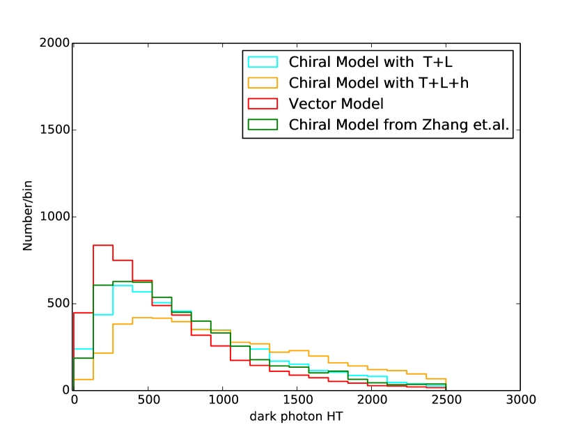
(a)

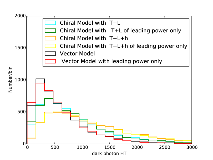
(b)

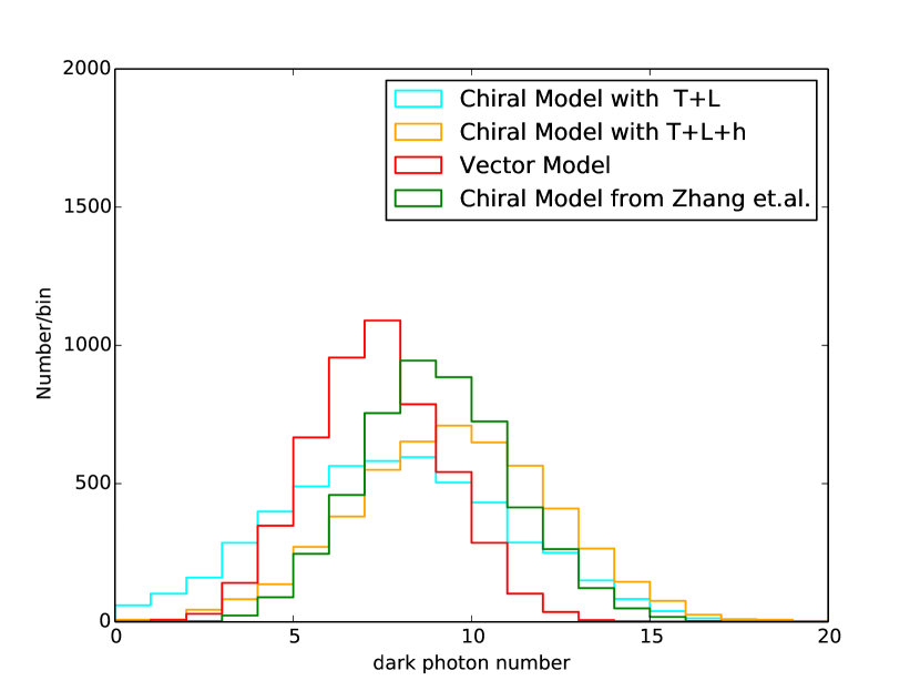
(c)

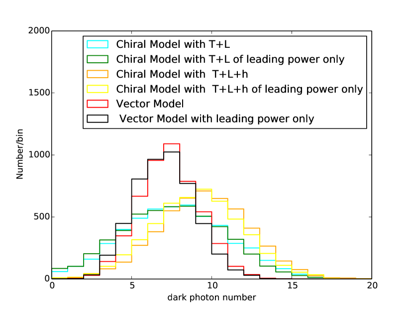
(d)

Figure 2: Dark shower with Point A: $\alpha^{\prime}=0.3$, $m_{\chi}=0.7$ GeV, $m_{A^{\prime}}=0.4$ GeV, and $m_{h^{\prime}}=1.0$ GeV. “T”, “L”, “h” represent the types of splitting functions: “T” for $\chi_{s}\rightarrow\chi_{s^{\prime}}A^{\prime}_{T}$; “L” for $\chi_{s}\rightarrow\chi_{s^{\prime}}A^{\prime}_{L}$; “h” for $\chi_{s}\rightarrow\chi_{s^{\prime}}h^{\prime}$. “Leading power” denotes the splitting functions with leading power contributions, i.e. those scaling as $\frac{d{\mathcal{P}}}{dzdk_{T}^{2}}\sim\frac{1}{k_{T}^{2}}$. “Zhang et. al.” labels the splitting functions from Zhang:2016sll by Zhang et. al.

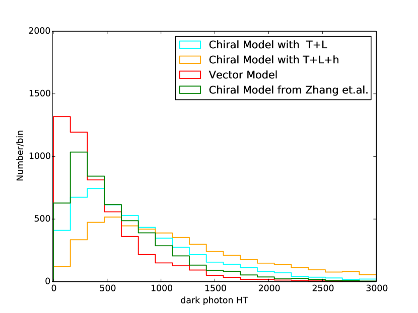
(a)

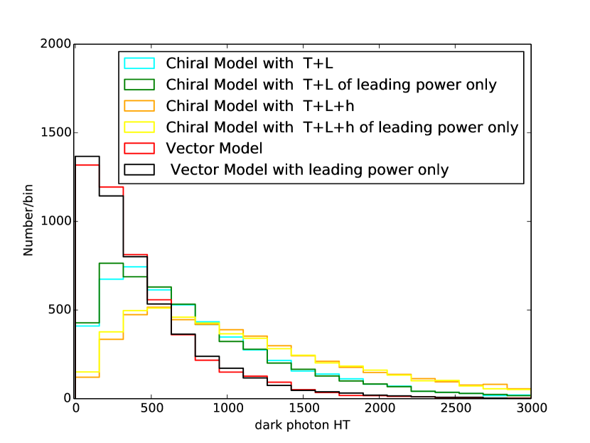
(b)

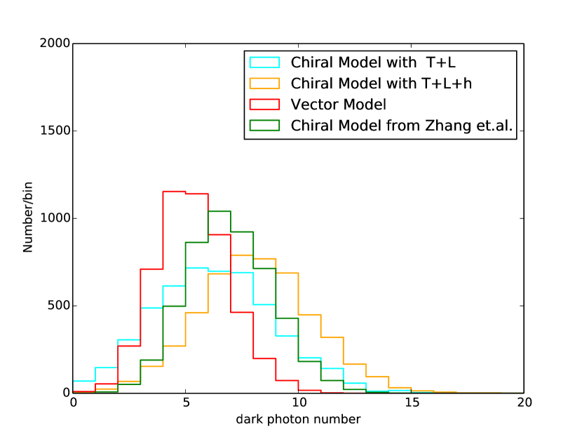
(c)

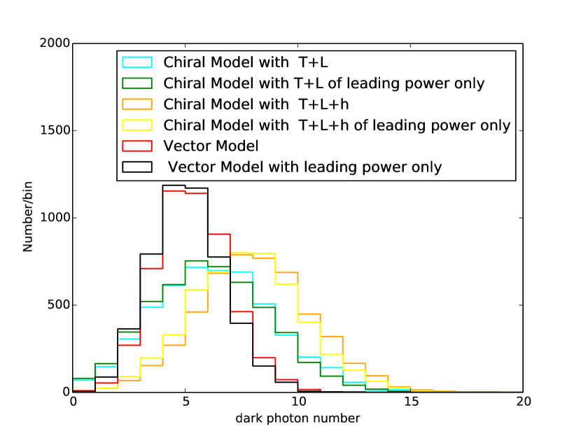
(d)

Figure 3: Same as Fig. 2 but with Point B: $\alpha^{\prime}=0.15$, $m_{\chi}=1.0$ GeV, $m_{A^{\prime}}=0.4$ GeV, and $m_{h^{\prime}}=1.0$ GeV.

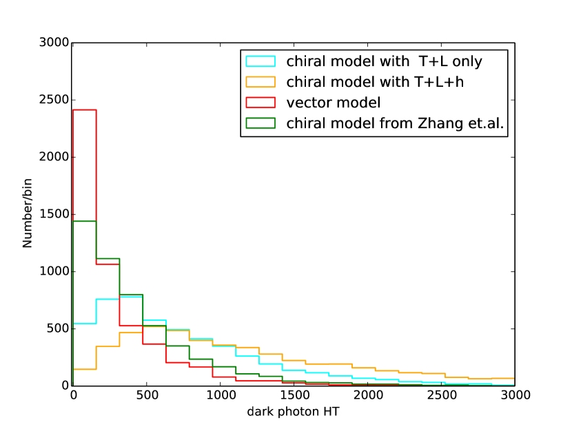
(a)

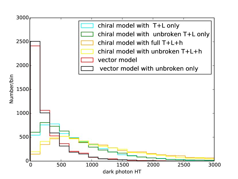
(b)

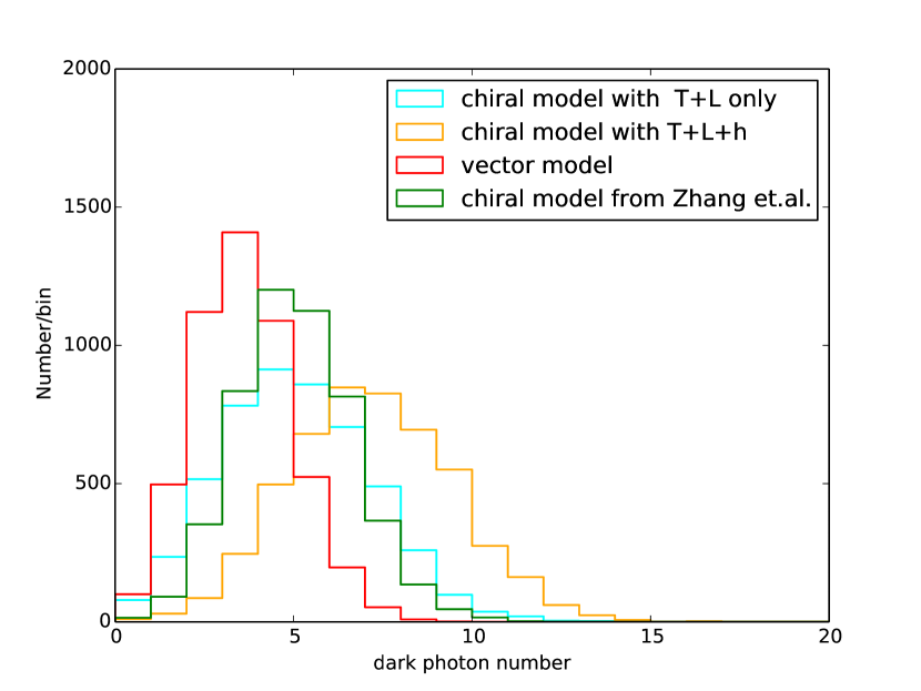
(c)

(d)

Figure 4: Same as Fig. 2 but with Point C: $\alpha^{\prime}=0.075$, $m_{\chi}=1.4$ GeV, $m_{A^{\prime}}=0.4$ GeV, and $m_{h^{\prime}}=1.4$ GeV.

Although we considered the dark photons as final states in generating Figs. 2, 3 and 4, the results for the dark photon number $n_{A}$ and for the scalar sum $H_{T}$ of the dark photon transverse momenta are basically identical, when the SM particles which the dark photons decay to are taken as final states. The reason is that almost all dark photons decay to SM particles before they reach the detectors at LHC with the kinematic mixing chosen in this work, as stated before. Moreover, the DM fermion produced in the hard process is highly boosted, so that all the particles in the dark shower are collimated, and contribute to the above observables. We illustrate this fact by presenting the plots with both the dark photons and the SM particles as final states in Fig. 5.

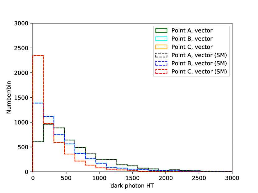
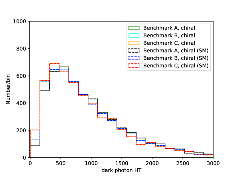
Figure 5: Comparison between $H_{T}$ with the dark photons as final states and that with the SM particles which the dark photons decay to as final states.

We then examine how the distributions of dark photons are affected by the cut imposed on the dark photon transverse momentum $p_{T}$ relative to the hard DM fermion. We plot in Fig. 6 the $n_{A}$ and $H_{T}$ distributions with and without the cut $p_{T}>10$ GeV for Point C. It is found that the $H_{T}$ distribution is not modified by the cut, whereas the $n_{A}$ distribution exhibits a dependence on the cut. It confirms the expectation that the number of dark photons is not an infrared-safe observable and contains an inherent theoretical uncertainty. Nevertheless, the difference between the Chiral and the Vector Model is not washed out after imposing the $p_{T}$ cut, because the distributions shift along the same direction.

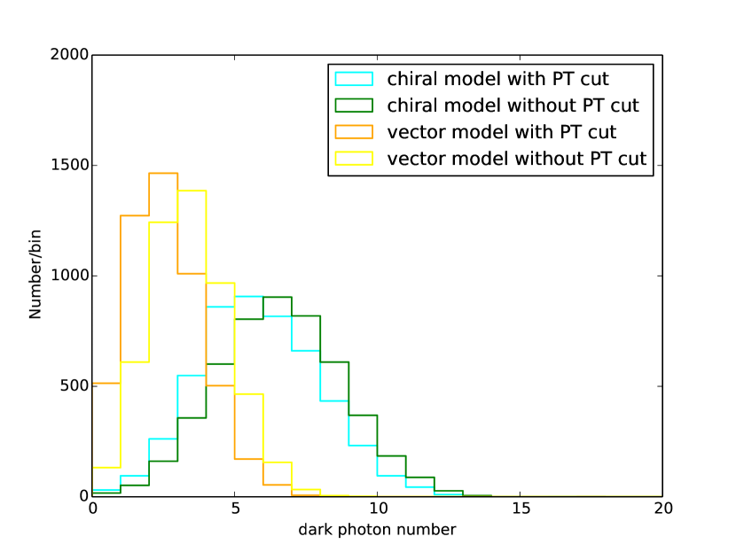
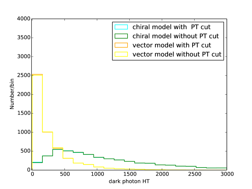
Figure 6: Distributions of dark photons without a cut and with a cut $p_{T}>10$ GeV for the Vector Model and the Chiral Model. The parameters are set to Point C.

To examine the shape of DM jets for each benchmark point, we cluster the final state particles radiated by a DM fermion using the anti-$k_{t}$ jet algorithm for the jet radius $R=2$ to determine the jet axis. We then average the energy deposit over $10^{4}$ DM jet events with respect to the distance to the jet axis. The jet profile is then described by the variable $f_{E}(r)$, defined as the energy fraction outside the cone with the radius $r<R$. The distributions of $f_{E}(r)$ from the Vector and Chiral Models for the three benchmark points are displayed in the left panel of Fig. 7, which descend from $f_{E}(r=0)=1$ to $f_{E}(r=R)=0$ following different curves. We notice that the jets are broader in the Chiral Model than in the Vector Model, since longitudinally polarized dark photons and dark Higgs bosons without the soft singularity in the momentum fraction $z$ can attain larger transverse momentum $k_{T}$ compared with transversely polarized dark photons, according to the Sudakov form factor in Eq. (3). In the right panel, we exhibit the jet profile for the point A with different DM energies. It is seen that the jet profile is mainly determined by the DM fermion chirality, and almost independent of the DM energy. This observation can be understood via the resummation formalism for the jet energy profile Li:2011hy , whose behavior is mainly determined by the $r$-dependent and energy-independent double logarithm. It implies that the jet profile is an appropriate observable for differentiating the DM fermion chirality.

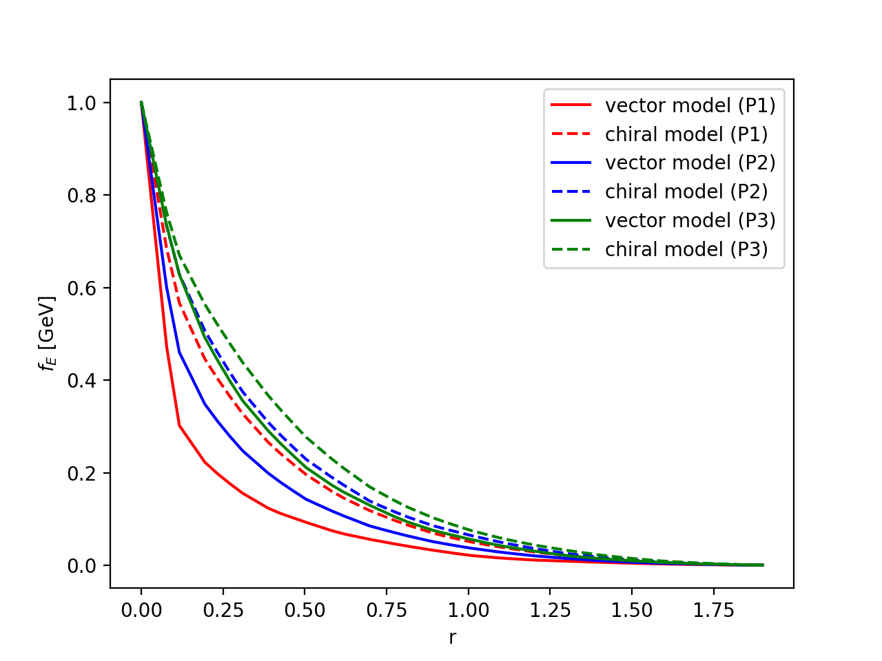
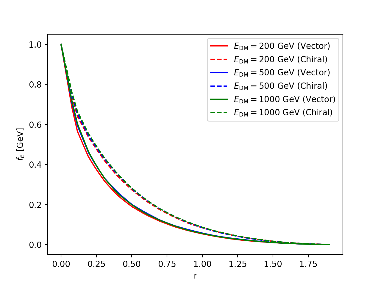
Figure 7: Left panel: energy profiles of DM jets for three benchmark points in the mono-jet channel ($p_{T}(j)>200$ GeV) at 14 TeV LHC. Right panel: energy profiles of DM jets for Point A with different DM energies.

V Conclusion

In this paper we investigated the dark shower patterns generated by energetic light DM fermions with different interactions to the dark photons at the LHC, evaluating the three observables explicitly, the scalar sum of dark photon transverse momenta, the dark photon number, and the energy profile of DM jets. Our work was motivated by the connection of the DM chiral property under a dark $U(1)$ gauge group to the mass origin of the dark sector, which could be realized at least in the simple Chiral and Vector Models considered here. It was shown that the DM chirality can indeed be distinguished by measuring the dark shower patterns: the shower is dominated by soft transversely polarized dark photons in the Vector Model, while it contains extra energetic longitudinally polarized dark photons and dark Higgs bosons in the Chiral Model. Especially, the jet energy profile, mainly determined by the DM fermion chirality and almost independent of the DM energy, seems to be an appropriate observable for the purpose.

Compared with the literatures on this subject, we have derived the complete set of $1\rightarrow 2$ splitting functions with the DM fermion as the initial state in the “DM fermion+dark $U(1)$” scenario. Based on these splitting functions, our implementation of the dark shower exhibits several novelties, making the analysis more accurate and valuable:

1. We specified the helicities of the DM fermions in the splitting functions and stressed that this specification is important for the Chiral Model, especially when the Yukawa coupling is comparable to the dark gauge coupling.

2. We analyzed the effects of the dark Higgs boson in different limits of the dark Higgs mass.

3. We included the symmetry breaking effects in the dark shower through a class of new splitting functions at power of $\frac{m^{2}}{k_{T}^{2}}$, though their effects on the shower patterns were found to be minor in general.

With the framework being solidly built up for correctly modeling the dark shower phenomena, we plan to carry out a careful collider analysis and related searching strategies in the forthcoming paper. It is also obvious that our formalism can be applied to more complicated and realistic models, and extended to include splittings of other initial particles, such as dark Higgs bosons, dark photons, etc..Ẇe will address these subjects in future publications.

Acknowledgements We thank the discussions with Tao Han, Myeonghun Park, Brock Tweedie and Mengchao Zhang. This work was partly supported in part by National Research Foundation of Korea (NRF) Research Grant NRF-2015R1A2A1A05001869 (PK, TM), and by the Ministry of Science and Technology of R.O.C. under Grant No. MOST-104-2112-M-001-037-MY3.

Appendix A Examples of Splitting Function Calculation

We take the processes $\chi_{s}\rightarrow\chi_{-s}A^{\prime}_{L}$ and $\chi_{s}\rightarrow\chi_{s}A^{\prime}_{L}$ in Fig. 8 as examples to demonstrate how to calculate the splitting functions for $A\rightarrow B+C$. We follow the methods in Ref. Chen:2016wkt basically by imposing the GEG, in which the amplitudes involving longitudinal vector bosons are derived by summing over both the Goldstone components and the remnant gauge components. To evaluate the collinear splitting amplitudes and the splitting functions, the total amplitude for a physical process should be factorized into the form

$$i{\mathcal{M}}=i{\mathcal{M}}_{split}\frac{i}{k_{A}^{2}-m_{A}^{2}}i{\mathcal{M}}_{hard}+\text{power\ suppressed}.$$ (16)

The collinear splitting function is then related to the splitting amplitude $i{\mathcal{M}}_{split}$ via

$$\frac{d{\mathcal{P}}}{dzdk_{T}^{2}}=\frac{1}{16\pi^{2}}z\bar{z}\frac{\overline{|{\mathcal{M}}_{split}|^{2}}}{\tilde{k}_{T}^{4}}.$$ (17)

To satisfy the factorization condition in Eq. (16), we need to write the fermion propagator of the initial virtual state as

$$\frac{\not{k}+m_{\chi}}{k^{2}-m_{\chi}^{2}}=\frac{\sum_{s}u^{0}_{s}(k)\bar{u}^{0}_{s}(k)}{k^{2}-m_{\chi}^{2}}+{\cal O}\left(\frac{1}{E}\right),$$ (18)

with $u^{0}_{s}(k)$ being the “on-shell” wave functions,

$$u^{0}_{-}(k)=\sqrt{E+|\vec{k}|}\left({\begin{array}[]{c}\xi_{-}\\ \frac{m_{\chi}}{E+|\vec{k}|}\xi_{-}\end{array}}\right)\hskip 28.45274ptu^{0}_{+}(k)=\sqrt{E+|\vec{k}|}\left({\begin{array}[]{c}\frac{m_{\chi}}{E+|\vec{k}|}\xi_{+}\\ \xi_{+}\end{array}}\right).$$

The factorization form makes clear that only the “on-shell” wave functions contribute nontrivially to the splitting amplitude $i{\mathcal{M}}_{split}$ and then to the collinear splitting function.

Figure 8: The $\chi\rightarrow\chi A^{\prime}$ splitting function.

We now compute the amplitude for $\chi_{s_{1}}\rightarrow\chi_{s_{2}}A_{L}^{\prime}$,

$$i{\mathcal{M}}_{\chi_{s_{1}}\rightarrow\chi_{s_{2}}A_{L}^{\prime}}=i{\mathcal{M}}_{\chi_{s_{1}}\rightarrow\chi_{s_{2}}\phi^{\prime}}+\text{phase}\cdot i{\mathcal{M}}_{\chi_{s_{1}}\rightarrow\chi_{s_{2}}A_{n}^{\prime}},$$ (19)

where the relative phase between the two amplitudes ${\mathcal{M}}_{\chi_{s_{1}}\rightarrow\chi_{s_{2}}\phi^{\prime}}$ and ${\mathcal{M}}_{\chi_{s_{1}}\rightarrow\chi_{s_{2}}A_{n}^{\prime}}$ can be obtained in the same way as Eq. (B16) in Ref. Chen:2016wkt . We define the covariant derivative $D_{\mu}\Phi^{\prime}=(\partial_{\mu}-ig^{\prime}Q_{\Phi^{\prime}}A_{\mu}^{\prime})\Phi^{\prime}$ with $g^{\prime}Q_{\Phi^{\prime}}>0$, by means of which the mixing Lagrangian becomes $-m_{A^{\prime}}\partial_{\mu}\phi^{\prime}A^{{}^{\prime}\mu}$ with a minus sign. The phase is then given by

$$\text{phase}=\left\{\begin{array}[]{rcl}-i&&\text{for incoming momentum},\\ i&&\text{for outgoing momentum}.\end{array}\right.$$

We specify the helicities, and divide the splittings into the helicity-flipping one $\chi_{s}\rightarrow\chi_{-s}A^{\prime}_{L}$ (leading power) and the helicity-conserving one $\chi_{s}\rightarrow\chi_{s}A^{\prime}_{L}$ (next-to-leading power). The $\chi_{s}\rightarrow\chi_{-s}A^{\prime}_{L}$ splitting amplitude is written as

$$i{\mathcal{M}}^{\chi_{s}\rightarrow\chi_{-s}A^{\prime}_{L}}_{split}=i\sqrt{2}g^{\prime}\frac{m_{\chi}}{m_{A^{\prime}}}Q_{\Phi^{\prime}}\bar{u}^{0}_{-s}(k_{B})\gamma_{5}u^{0}_{s}(k_{A})+{\cal O}\left(\frac{m}{E}\right),$$ (21)

in which the power suppressed term comes from the gauge component contribution. The Goldstone component leads to

$$i{\mathcal{M}}^{\chi_{s}\rightarrow\chi_{-s}A^{\prime}_{L}}_{split}=i\sqrt{2}g^{\prime}\frac{m_{\chi}}{m_{A^{\prime}}}Q_{\Phi^{\prime}}\frac{1}{\sqrt{2\bar{z}}}k_{T},$$ (22)

via which we obtain, according to Eq. (17), the splitting function for $\chi_{s}\rightarrow\chi_{-s}A^{\prime}_{L}$ given in Eq. (10).

The $\chi_{s}\rightarrow\chi_{s}A^{\prime}_{L}$ splitting amplitude is decomposed into

$$i{\mathcal{M}}^{\chi_{s}\rightarrow\chi_{s}A^{\prime}_{L}}_{split} = i{\mathcal{M}}^{\chi_{s}\rightarrow\chi_{s}A^{\prime}_{n}}_{split}+\text{phase}\cdot i{\mathcal{M}}^{\chi_{s}\rightarrow\chi_{s}\phi^{\prime}}_{split},$$ (23)

with

$$i{\mathcal{M}}^{\chi_{s}\rightarrow\chi_{s}A^{\prime}_{n}}_{split} = ig^{\prime}\sum_{s=L,R}Q_{s}\bar{u}^{0}_{s}(k_{B})\gamma^{\mu}P_{s}u^{0}_{s}(k_{A})\epsilon_{\mu},$$

$$i{\mathcal{M}}^{\chi_{s}\rightarrow\chi_{s}\phi^{\prime}}_{split} = i\sqrt{2}g^{\prime}\frac{m_{\chi}}{m_{A^{\prime}}}Q_{\Phi}\bar{u}^{0}_{s}(k_{B})\gamma_{5}u^{0}_{s}(k_{A}),$$ (24)

where $P_{s}$ is the operator to project out the left-handed chirality ($P_{L}=\frac{1-\gamma_{5}}{2}$) or the right-handed chirality $P_{R}=\frac{1+\gamma_{5}}{2}$. A straightforward derivation yields the splitting amplitudes

$$i{\mathcal{M}}^{\chi_{L}\rightarrow\chi_{L}A^{\prime}_{L}}_{split} = ig^{\prime}m_{A^{\prime}}\frac{2}{z\sqrt{\bar{z}}}\left(Q_{L}\bar{z}+\frac{z^{2}m_{\chi}^{2}}{2m_{A^{\prime}}^{2}}(Q_{L}-Q_{R})\right),$$

$$i{\mathcal{M}}^{\chi_{R}\rightarrow\chi_{R}A^{\prime}_{L}}_{split} = ig^{\prime}m_{A^{\prime}}\frac{2}{z\sqrt{\bar{z}}}\left(Q_{R}\bar{z}-\frac{z^{2}m_{\chi}^{2}}{2m_{A^{\prime}}^{2}}(Q_{L}-Q_{R})\right).$$

Combining the $s=R(+\frac{1}{2})$ and $s=L(-\frac{1}{2})$ pieces, we have

$$i{\mathcal{M}}^{\chi_{s}\rightarrow\chi_{s}A^{\prime}_{L}}_{split} = ig^{\prime}m_{A^{\prime}}\frac{1}{z\sqrt{\bar{z}}}\left(2Q_{s}\bar{z}+(-1)^{s+\frac{1}{2}}\frac{z^{2}m_{\chi}^{2}}{m_{A^{\prime}}^{2}}Q_{\Phi^{\prime}}\right).$$ (25)

Inserting the above expression into Eq. (17) leads to the splitting function for $\chi_{s}\rightarrow\chi_{s}A^{\prime}_{L}$ in Eq. (13),

$$\frac{d{\mathcal{P}}}{dzdk_{T}^{2}}(\chi_{s}\rightarrow\chi_{s}A^{\prime}_{L})=\frac{\alpha^{\prime}}{2\pi}\frac{1}{2z}\left(2Q_{s}\bar{z}+(-1)^{s+\frac{1}{2}}\frac{z^{2}m_{\chi}^{2}}{m_{A^{\prime}}^{2}}Q_{\Phi^{\prime}}\right)^{2}\frac{m_{A^{\prime}}^{2}}{\tilde{k}_{T}^{4}}.$$ (26)

References

- (1) B. W. Lee and S. Weinberg, Phys. Rev. Lett. 39, 165 (1977).
- (2) G. Jungman, M. Kamionkowski and K. Griest, Phys. Rept. 267, 195 (1996).
- (3) O. Adriani et al. [PAMELA Collaboration], Nature 458, 607 (2009).
- (4) D. N. Spergel and P. J. Steinhardt, Phys. Rev. Lett. 84, 3760 (2000).
- (5) N. Arkani-Hamed, D. P. Finkbeiner, T. R. Slatyer and N. Weiner, Phys. Rev. D 79, 015014 (2009).
- (6) M. Cirelli, M. Kadastik, M. Raidal and A. Strumia, Nucl. Phys. B 813, 1 (2009) Addendum: [Nucl. Phys. B 873, 530 (2013)].
- (7) N. Arkani-Hamed and N. Weiner, JHEP 0812, 104 (2008).
- (8) J. Alexander et al., arXiv:1608.08632 [hep-ph].
- (9) S. Baek, P. Ko and W. I. Park, JHEP 1307, 013 (2013) doi:10.1007/JHEP07(2013)013 [arXiv:1303.4280 [hep-ph]].
- (10) P. Ko, New Phys. Sae Mulli 66, no. 8, 966 (2016). doi:10.3938/NPSM.66.966
- (11) B. Holdom, Phys. Lett. 166B, 196 (1986).
- (12) T. Cohen, M. Lisanti, H. K. Lou and S. Mishra-Sharma, JHEP 1711, 196 (2017).
- (13) J. Chen, T. Han and B. Tweedie, JHEP 1711, 093 (2017).
- (14) M. Buschmann, J. Kopp, J. Liu and P. A. N. Machado, JHEP 07, 045 (2015).
- (15) M. Zhang, M. Kim, H. S. Lee and M. Park, arXiv:1612.02850 [hep-ph].
- (16) N. F. Bell, Y. Cai and R. K. Leane, JCAP 1701, no. 01, 039 (2017).
- (17) H. Ruegg and M. Ruiz-Altaba, Int. J. Mod. Phys. A 19, 3265 (2004).
- (18) F. Kahlhoefer, K. Schmidt-Hoberg, T. Schwetz and S. Vogl, JHEP 1602, 016 (2016).
- (19) T. Sjöstrand et al., Comput. Phys. Commun. 191, 159 (2015).
- (20) S. Alekhin et al., Rept. Prog. Phys. 79, no. 12, 124201 (2016).
- (21) Y. Kitadono and H. n. Li, Phys. Rev. D 89, no. 11, 114002 (2014); Phys. Rev. D 93, no. 5, 054043 (2016).
- (22) H. n. Li, Z. Li and C.-P. Yuan, Phys. Rev. Lett. 107, 152001 (2011); Phys. Rev. D 87, 074025 (2013).