”Blinking eigenvalues” of the Steklov problem generate the continuous spectrum in a cuspidal domain

Abstract.

We study the Steklov spectral problem for the Laplace operator in a bounded domain $\Omega\subset{\mathbb{R}}^{d}$, $d\geq 2$, with a cusp such that the continuous spectrum of the problem is non-empty, and also in the family of bounded domains $\Omega^{\varepsilon}\subset\Omega$, $\varepsilon>0$, obtained from $\Omega$ by blunting the cusp at the distance of $\varepsilon$ from the cusp tip. While the spectrum in the blunted domain $\Omega^{\varepsilon}$ consists for a fixed $\varepsilon$ of an unbounded positive sequence $\{\lambda_{j}^{\varepsilon}\}_{j=1}^{\infty}$ of eigenvalues, we single out different types of behavior of some eigenvalues as $\varepsilon\to+0$: in particular, stable, blinking, and gliding families of eigenvalues are found. We also describe a mechanism which transforms the family of the eigenvalue sequences into the continuous spectrum of the problem in $\Omega$, when $\varepsilon\to+0$.

1. Introduction.

1.1. Formulation of the problems.

Let $\Omega$ be a domain in ${\mathbb{R}}^{n}$, $n\geq 2$, with compact closure $\overline{\Omega}$ and boundary $\partial\Omega$ which is smooth everywhere except at the origin ${\mathcal{O}}$ of the Cartesian coordinate system $x=(y,z)\in{\mathbb{R}}^{n-1}\times{\mathbb{R}}$ (Fig. 1.1,a). In a neighborhood of the point ${\mathcal{O}}$ the domain $\Omega$ coincides with the cusp

(1.1) $$\Pi^{d}=\{x=(y,z)\,:\,z\in(0,d),\eta=z^{-m}y\in\omega\}\ ,\ \ d>0,$$

where $m>1$ is the sharpness exponent of the cusp and the cross-section $\omega$ is a domain in ${\mathbb{R}}^{n-1}$ bounded by a smooth $(n-2)$-dimensional closed surface $\partial\omega$.

First of all, we consider the Steklov problem for the Laplace operator

(1.2) $$-\Delta u(x) = \lambda u(x),\,x\in\Omega,\ \ \ \partial_{\nu}u(x)=\lambda u(x),\,x\in\partial\Omega,$$

where $\partial_{\nu}$ is the outward normal derivative and $\lambda$ is the spectral parameter.

We introduce the Hilbert space ${\mathcal{H}}$ endowed with the norm

(1.3) $$\|u;{\mathcal{H}}\|=\big{(}\|\nabla u;L^{2}(\Omega)\|^{2}+\|u;L^{2}(\partial\Omega)\|^{2}\big{)}^{1/2}$$

and contained in the Sobolev space $H^{1}(\Omega)$. Then, the integral identity corresponding to the problem (1.2) reads as

(1.4) $$(\nabla u,\nabla v)_{\Omega}=\lambda(u,v)_{\Omega}\hskip 28.45274pt\forall\,v\in{\mathcal{H}},$$

see [9]. Here, $\nabla$ is the gradient, $(\ \,,\ )_{\Upsilon}$ is the natural scalar product in the Lebesgue space $L^{2}(\Upsilon)$, while the scalar product in ${\mathcal{H}}$ generated by the norm (1.3) will be denoted by $\langle\ \,,\ \rangle$ in the following. Moreover, we define the operator ${\mathcal{S}}:{\mathcal{H}}\to{\mathcal{H}}$ and the new spectral parameter $\mu$ by

(1.5) $$\langle{\mathcal{S}}u,v\rangle = (u,v)_{\partial\Omega}\hskip 28.45274pt\forall\,u,v\in{\mathcal{H}},$$

(1.6) $$\mu = (1+\lambda)^{-1},$$

and by these relations the problem (1.4) is converted to the abstract equation

(1.7) $${\mathcal{S}}u=\mu u\hskip 28.45274pt\mbox{in}\ {\mathcal{H}}.$$

Clearly, the operator ${\mathcal{S}}$ is positive definite, symmetric and continuous, and, therefore, self-adjoint.

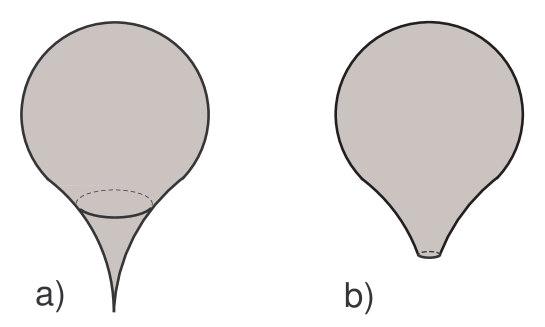
Figure 1.1. a) Cuspidal domain, b) domain with blunted cusp.

If we assume for a while that $m\leq 1$ in (1.1), the boundary $\partial\Omega$ becomes Lipschitz and the essential spectrum of ${\mathcal{S}}$ consists only of the single point $\mu=0$ due to the compactness of the embedding ${\mathcal{H}}=H^{1}(\Omega)\subset L^{2}(\Omega)$, cf. [1, Thm. 10.1.5.]. The remaining part of the spectrum is discrete and forms a positive sequence converging to zero so that according to the relation (1.6) the whole spectrum $\sigma$ of the problem (1.4) (the Steklov problem (1.2)) consists of an unbounded positive sequence of normal eigenvalues. As verified in [18], the spectrum remains discrete, if $m<2$.

However, in the case $m\geq 2$ the above-mentioned embedding ${\mathcal{H}}\subset L^{2}(\Omega)$ loses its compactness, see e.g. [18] and [11], and hence the continuous components $\sigma_{\rm co}$ of the spectra of the operator ${\mathcal{S}}$ and the Steklov problem become non-empty. The component $\sigma_{\rm co}=[\lambda_{\dagger},+\infty)$ will be described explicitly in Section 4 for the most interesting case

(1.8) $$m=2,$$

where the positive cut-off value $\lambda_{\dagger}$ will be obtained from (2.10). Note that in the case $m>2$ it was shown in [18] that $\lambda_{\dagger}=0$ and $\sigma_{\rm co}=[0,+\infty)$; this case will not be considered in the present paper.

Blunting the cuspidal tip makes the boundary Lipschitz again, see Fig. 1.1,b. We consider the simplest truncation

(1.9) $$\Omega^{\varepsilon}=\Omega\smallsetminus\overline{\Pi^{\varepsilon}}\hskip 28.45274pt\mbox{with a small}\ \varepsilon\in(0,d)$$

and the mixed boundary-value problem

(1.10) $$-\Delta u^{\varepsilon}(x) = 0,\hskip 42.67912ptx\in\Omega^{\varepsilon},$$

(1.11) $$\partial_{\nu}u^{\varepsilon}(x) = \lambda^{\varepsilon}u^{\varepsilon}(x),\hskip 11.38092ptx\in(\partial\Omega)^{\varepsilon}=\partial\Omega^{\varepsilon}\smallsetminus\overline{\omega^{\varepsilon}},$$

(1.12) $$u^{\varepsilon}(x) = 0,\hskip 42.67912ptx\in\omega^{\varepsilon},$$

with the artificial Dirichlet condition in the end $\omega^{\varepsilon}=\{x\in\Pi^{d}\,:\,z=\varepsilon\}$. Other truncation surfaces and types of the artificial boundary condition will be discussed in Section 4.

The operator formulation of the problem (1.10)–(1.12) will be given in Section 4, but is is clear that its spectrum $\sigma^{\varepsilon}$ is discrete and consists of the positive unbounded sequence of eigenvalues

(1.13) $$0<\lambda_{1}^{\varepsilon}<\lambda_{2}^{\varepsilon}\leq\lambda_{3}^{\varepsilon}\leq\ldots\leq\lambda_{m}^{\varepsilon}\leq\ldots\to+\infty.$$

The main goal of our paper is to describe the abnormal behavior of some entries in (1.13), when $\varepsilon\to+0$ and the domain sharpens into a cusp. Furthermore, we will find a mechanism transforming the family of the sequences (1.13) into the continuous spectrum $\sigma$ of the original Steklov problem (1.2).

We will not investigate the asymptotics of all eigenvalues (1.13) but only some of them. First, in Section 4.3 we find families of eigenvalues which have the property that for some $\lambda^{\sf tr}$ and any small enough $\varepsilon>0$, the $c\varepsilon$-neighborhood of $\lambda^{\sf tr}$ contains an eigenvalue belonging to the sequence (1.13), for some positive constant $c$ independent of $\varepsilon$. For brevity, we call such families ”stable eigenvalues”. (In Section 4.1,$3^{\circ}$, we make a remark showing that every $\lambda>\lambda_{\dagger}$ indeed is an eigenvalue of the problem (1.10)–(1.12) for some $\varepsilon$.)

Moreover, Theorem 4.3 shows that any point $\lambda>\lambda_{\dagger}$ becomes a ”blinking eigenvalue” (Section 4.1,$2^{\circ}$) when $\varepsilon\to+0$, i.e. there exists a positive sequence $\{\varepsilon_{k}\}_{k=1}^{\infty}=\{\varepsilon_{k}(\lambda)\}_{k=1}^{\infty}$ tending to 0 such that for $\varepsilon=\varepsilon_{k}$, the $c_{\lambda}\varepsilon_{k}$-neighborhood of $\lambda$ contains an entry $\lambda_{m_{k}}^{\varepsilon_{k}}$, where $m_{k}=m_{k}(\lambda)$. (However, for $\varepsilon\not=\varepsilon_{k}$, there is no guarantee of this family staying near $\lambda$. The number $\lambda$ becomes a true eigenvalue of the problem (1.10)–(1.12) for some $\varepsilon$ close to any entry of the sequence $\{\varepsilon_{k}\}_{k=1}^{\infty}$). This fact can obviously be used for the construction of a singular Weyl sequence for the operator ${\mathcal{S}}$ at the point (1.6) (Section 5.1). It is a remarkable fact that the structure of the elements of this singular sequence is quite different from the one used in [18] for the continuous spectrum $\sigma_{\rm co}$.

One more strange phenomenon on the behavior of the eigenvalues of the problem (1.10)–(1.12) will be described in Section 4.1,$3^{\circ}$, namely so called ”gliding eigenvalues”. We will detect a set of eigenvalues $\lambda_{m_{k}(\varepsilon)}^{\varepsilon}$, with changing numbers $m_{k}(\varepsilon)$, falling down at a high speed $O\big{(}\varepsilon^{-1}|\ln\varepsilon|^{-1}(\lambda_{m(\varepsilon)}^{\varepsilon}-\lambda_{\dagger})\big{)}$ as $\varepsilon\to+0$. The speed however declines while approaching the threshold, which produces a smooth touchdown of $\lambda_{m(\varepsilon)}^{\varepsilon}$ at $\lambda_{\dagger}$. Furthermore, these eigenvalues ”sweep” the semi-axis $(\lambda_{\dagger},+\infty)$ many times, when $\varepsilon\to+0$ and the Lipschitz domain $\Omega^{\varepsilon}$ becomes cuspidal. (Notice that the ”blinking” and ”gliding” behaviors do not constitute a classification or define separate values of $\varepsilon$ or $\lambda$ — they are just different aspects among the families of eigenvalues.)

The number $\lambda_{\dagger}$ still belongs to the continuous spectrum, since, according to the general results in [5, 15], see also [7, Ch. 10], eigenvalues of infinite multiplicity do not appear in elliptic problems in cuspidal domains so that the essential and continuous spectra coincide and thus the latter is also a closed set.

2. Known facts.

2.1. Formal asymptotic procedure.

For an eigenfunction of the problem (1.2), we introduce the standard asymptotic ansatz in the analysis of thin domains, which has in particular been used in [18, 20]

(2.1) $$u(y,z)=w(z)+W(\eta,z)+\ldots,$$

where $w$ and $W$ are the power-law functions

(2.2) $$w(z)=z^{\tau}w_{0}\ ,\ \ W(\eta,z)=z^{\tau+2}W_{0}(\eta),$$

$\eta=(\eta_{1},\ldots,\eta_{n-1})=z^{-2}y$ are the stretched coordinates in (1.1), and the dots stand for higher-order terms to be estimated in Section 4. We insert (2.1), (2.2) to the restriction of the problem (1.2) on the cusp (1.1) and collect the terms of order $z^{\tau-2}$ in the Laplace equation, and thus obtain the $(n-1)$-dimensional Poisson equation with the parameter $z>0$,

(2.3) $$-\Delta_{\eta}W_{0}(\eta)=F(\eta):=z^{2-\tau}\partial_{z}^{2}w(z)\ ,\ \ \eta\in\omega.$$

The unit outward normal vector on the lateral side $\Gamma^{d}=\{x\,:\,\eta\in\partial\omega,z\in(0,d)\}$ of the cusp equals

(2.4) $$\nu(y,z)=\big{(}1+4z^{2}|\eta\cdot\nu^{\prime}(\eta)|^{2}\big{)}^{-1/2}\big{(}\nu^{\prime}(\eta),-2z\eta\cdot\nu^{\prime}(\eta)\big{)},$$

where $\nu^{\prime}=(\nu_{1}^{\prime},\ldots,\nu_{n-1}^{\prime})$ is the normal on the boundary $\partial\omega\subset{\mathbb{R}}^{n-1}$ and $|\nu^{\prime}|=1$. Thus, extracting terms of order $z^{\tau}$ from the Steklov condition yields the boundary condition

(2.5) $$\partial_{\nu^{\prime}}W_{0}(\eta)=G(\eta):=z^{-\tau}\big{(}\lambda w(z)+2z\eta\cdot\nu^{\prime}(\eta)\partial_{z}w(z)\big{)}\ ,\ \ \eta\in\partial\omega,$$

where $\partial_{z}=\partial/\partial z$, $\partial_{\nu^{\prime}}=\nu^{\prime}\cdot\nabla_{\eta}$ and the central dot stands for the scalar product in the Euclidean space. According to (2.2), the right-hand sides of (2.3) and (2.5) are indeed independent of $z$. The combatibility condition in the Neumann problem (2.3), (2.5) is written as

(2.6) $$0 = \int\limits_{\omega}F(\eta)d\eta+\int\limits_{\partial\omega}G(\eta)ds_{\eta}$$

$$= z^{2-\tau}\big{(}|\omega|\partial_{z}^{2}w(z)+\lambda|\partial\omega|w(z)+2(n-1)|\omega|^{-1}z\partial_{z}w(z)\big{)}$$

with the volume $|\omega|={\rm mes}_{n-1}\omega$ and the area $|\partial\omega|={\rm mes}_{n-2}\partial\omega$. We multiply (2.6) by $z^{2n+\tau}$ and, as a result, obtain the ordinary differential equation of Euler type

(2.7) $$-\partial_{z}\big{(}z^{2(n-1)}|\omega|\partial_{z}w(z)\big{)}=\Lambda z^{2(n-2)}|\partial\omega|w(z)\ ,\ \ z>0,$$

with the coefficient

(2.8) $$\Lambda=\frac{|\partial\omega|}{|\omega|}\lambda.$$

It has the solutions

(2.9) $$w_{\pm}(z)=w_{0}z^{\tau_{\pm}}\ \ \mbox{with}\ \tau_{\pm}=-\Big{(}n-\frac{3}{2}\Big{)}\pm\sqrt{\Big{(}n-\frac{3}{2}\Big{)}^{2}-\Lambda}.$$

The imaginary parts of both exponents $\tau_{\pm}$ are nonzero provided

(2.10) $$\Lambda>\big{(}n-\frac{3}{2}\Big{)}^{2}=:\Lambda_{\dagger}\ \ \Leftrightarrow\ \ \lambda>\lambda_{\dagger}:=\Big{(}n-\frac{3}{2}\Big{)}^{2}\frac{|\omega|}{|\partial\omega|},$$

but both $\tau_{\pm}$ are real in the case $\lambda<\lambda_{\dagger}$. Finally, for $\lambda=\lambda_{\dagger}$, the general solution of (2.7) is

$$w(z)=z^{-n+3/2}(c_{0}+c_{1}\ln z).$$

In Section 3 it will be convenient to set

(2.11) $$w_{\pm}(z)=w_{0}z^{-n+3/2}(1\pm i\ln z)\ \ \ \mbox{at}\ \lambda=\lambda_{\dagger}$$

so that we can write the general solution for every $\lambda\geq\lambda_{\dagger}$ as

(2.12) $$w(z)=b_{+}w_{+}(z)+b_{-}w_{-}(z)\ \ \ \mbox{with}\ b_{\pm}\in{\mathbb{C}}.$$

The normalization factor $w_{0}$ of (2.9) and (2.12) will be fixed in the formulas (3.3), (3.5) of Section 3.1.

Since the compatibility condition (2.6) is satisfied by the function (2.12), the Neumann problem (2.3), (2.5) has a solution $W$ which is defined up to an additive constant and becomes unique by requiring the orthogonality condition

(2.13) $$\int\limits_{\omega}W_{0}(\eta)d\eta=0.$$

2.2. The spectrum of the Steklov problem.

The following result was proven in [18] by constructing Weyl singular sequences for $\lambda>\lambda_{\dagger}$ and parametrices for the Steklov problem operator in the case $\lambda\in[0,\lambda_{\dagger})$.

Theorem 2.1.

The continuous spectrum $\sigma_{\rm co}$ of the Steklov problem (1.2) in the cuspidal domain $\Omega$ with the sharpness exponent (1.8) equals $[\lambda_{\dagger},+\infty)$, where the cut-off point $\lambda_{\dagger}$ is given in (2.10).

In other words, the essential spectrum of the operator ${\mathcal{S}}$ consists of the point $\mu=0$ and the continuous spectrum $(0,\mu_{\dagger}]$, where $\mu_{\dagger}=(1+\lambda_{\dagger})^{-1}$, according to (1.6).

Null is an eigenvalue of the problem (1.2), and the interval $(0,\lambda_{\dagger})$ below the continuous spectrum $\sigma_{\rm co}$ may contain other points of the discrete spectrum $\sigma_{\rm di}$. Furthermore, it was verified in [18] that in the mirror symmetric case

(2.14) $$\Omega=\{(y,z)\,:\,(-y_{1},y_{2},\ldots,y_{n-1},z\}\in\Omega\}$$

the point spectrum $\sigma_{\rm po}$ is non-empty and in particular it includes the unbounded monotone sequence

(2.15) $$0<\lambda_{1}^{+}<\lambda_{2}^{+}\leq\lambda_{3}^{+}\leq\ldots\leq\lambda_{p}^{+}\leq\ldots\to+\infty$$

of eigenvalues of the auxiliary problem

$$-\Delta u^{+}(x) = 0,\,x\in\Omega^{+},\ \ \ \partial_{\nu}u^{+}(x)=\lambda^{+}u^{+}(x),\,x\in(\partial\Omega)^{+},$$

$$u^{+}(x) = 0,\,x\in\Sigma=\partial\Omega^{+}\cap\Omega,$$

where $\Omega^{+}=\{x\in\Omega\,:\,y_{1}>0\}$ is the half-domain and $\Sigma$ is the artificial truncation surface.

2.3. Weak formulation of the inhomogeneous Steklov problem.

We fix the value of the parameter $\lambda$ in the problem

(2.16) $$-\Delta u(x)=f(x),\,x\in\Omega,\ \ \ \partial_{\nu}u(x)-\lambda u(x)=g(x),\,x\in\partial\Omega\smallsetminus{\mathcal{O}},$$

and introduce the space $V_{\beta}^{1}(\Omega)$ with the weighted norm

(2.17) $$\|u;V_{\beta}^{1}(\Omega)\|=\big{(}\|\nabla u;L_{\beta}^{2}(\Omega)\|^{2}+\|u;L_{\beta-1}^{2}(\Omega)\|^{2}+\|u;L_{\beta}^{2}(\partial\Omega)\|^{2}\big{)}^{1/2}$$

where $\beta\in{\mathbb{R}}$, $L_{\beta}(\Upsilon)$ is the weighted Lebesgue space with the norm

$$\|v;L_{\beta}(\Upsilon)\|=\|r^{\beta}v;L(\Upsilon)\|$$

and $r=|x|$ is the distance of $x$ from the cusp tip ${\mathcal{O}}$.

Lemma 2.2.

For every $u\in C_{c}^{\infty}(\overline{\Omega}\smallsetminus{\mathcal{O}})$ and compact subset $K$ of $\overline{\Omega}\smallsetminus{\mathcal{O}}$, there holds the inequality

(2.18) $$\|u;L_{\beta-1}^{2}(\Omega)\|+\|u;L_{\beta}^{2}\partial(\Omega)\|\leq c\big{(}\|\nabla u;L_{\beta}^{2}(\Omega)\|+\|u;L^{2}(K)\|\big{)},$$

where the constant $c$ depends on $\Omega$, $K$ and $\beta$ but not on $u$.

Proof. Replacing $u\mapsto r^{-\beta}u$ reduces the claim to the case $\beta=0$ which has been considered in [18, Sect. 2].   $\boxtimes$

We associate with the problem (2.16) the integral identity [9]

(2.19) $$(\nabla u,\nabla v)_{\Omega}-\lambda(u,v)_{\partial\Omega}=F(v)\hskip 28.45274pt\forall\,v\in V_{-\beta}^{1}(\Omega),$$

where $F\in V_{-\beta}^{1}(\Omega)^{*}$ is an (anti)linear functional in $V_{-\beta}^{1}(\Omega)$, for instance,

(2.20) $$F(v)=(f,v)_{\Omega}+(g,v)_{\partial\Omega}\ \ \mbox{with}\ f\in L_{\beta+1}^{2}(\Omega),\ g\in L_{\beta}^{2}(\partial\Omega).$$

According to (2.20), all terms in (2.19) are properly defined so that (2.19) defines a continuous mapping

(2.21) $$V_{\beta}^{1}(\Omega)\ni u\mapsto T_{\beta}(\lambda)u=F\in V_{-\beta}^{1}(\Omega)^{*}.$$

In [18] it is proven that the operator $T_{0}(\lambda)$ is Fredholm for $\lambda\in[0,\lambda_{\dagger})$ but loses this property for $\lambda\geq\lambda_{\dagger}$. Notice that the latter fact follows from the failure of the inclusion $z^{\tau_{\pm}}\in V_{0}^{1}(\Pi^{d})$ in the case (2.10). We remark that $T_{\beta}(\lambda)$ is still Fredholm, if $\lambda\geq\lambda_{\dagger}$ and $\beta\not=0$, although this fact will be of no use here.

2.4. Asymptotics of the solutions in the cusp.

We consider problem (2.19) with the right-hand side (2.20), where $\beta=-1$ and

(2.22) $$g=0,\ f\in L^{2}(\Omega).$$

The following assertion on the asymptotics of the solution of the Steklov problem (2.16) can be found in [20, Thm. 2.6].

Theorem 2.3.

Let $u\in V_{1}^{1}(\Omega)$ be a solution of the problem (2.21) with $\lambda\geq\lambda_{\dagger}$, $\beta=1$ and the right-hand side (2.20), (2.22). Then, $u$ has the representation

(2.23) $$u(x)=\widetilde{u}(x)+\chi(x)\big{(}w(z)+W(z^{-2}y,z)\big{)},$$

where the remainder $\widetilde{u}$ lives in $V_{-1}^{1}(\Omega)$ and $\chi$ is a smooth cut-off function,

(2.24) $$\chi=1\ \mbox{in}\ \Pi^{d/2}\ and\ \chi=0\ \mbox{in}\ \Omega\smallsetminus\Pi^{d}.$$

Moreover, $w$ is the linear combination (2.3) with some coefficients $b_{\pm}$ depending on $f$ and including the functions (2.9) in the case $\lambda>\lambda_{\dagger}$ and (2.11) in the case $\lambda=\lambda_{\dagger}$, while $W$ is determined by (2.2), (2.3), (2.5), (2.13). Furthermore, there holds the estimate

(2.25) $$\|\widetilde{u};V_{-1}^{1}(\Omega)\|+|b_{+}|+|b_{-}|\leq c\big{(}\|f;L^{2}(\Omega)\|+\|u;V_{1}^{1}(\Omega)\|\big{)}$$

with a coefficient $c$ independent of $f$ and $u$.

We emphasize that for $\lambda<\lambda_{\dagger}$, i.e., below the continuous spectrum $\sigma_{\rm co}$, the asymptotic form of the solutions of the problem (2.16) is different from that in Theorem 2.3.

Remark 2.4.

A direct calculation based on formulas (2.9), (2.11) and (2.2) shows that the function $\chi(w+W)$ in Theorem 2.3 lives in $V_{1}^{1}(\Omega)$ but does not belong to $V_{-1}^{1}(\Omega)$, if $|b_{+}|+|b_{-}|\not=0$. Note that the solution $W$ of the Neumann problem (2.3), (2.5) is determined up to the addentum

(2.26) $$z^{-n+3/2\pm i\tau_{0}}W_{\bullet}\ \ \mbox{with}\ \tau_{0}=\sqrt{\Big{(}n-\frac{3}{2}\Big{)}^{2}-\Lambda}$$

which is constant with respect to $\eta$. However, the term (2.26) belongs to both spaces $V_{\pm 1}^{1}(\Pi^{d})$ and thus can be omitted in (2.23). This explains why one requires the orthogonality condition (2.13) on $W_{0}$.   $\boxtimes$

Remark 2.5.

A solution $u$ of the problem (2.19) with data (2.22) belongs to the linear space $H_{\rm loc}^{2}(\overline{\Omega}\smallsetminus{\mathcal{O}})$. According to [20, Lem. 3.2] [[correct reference?]], the second derivatives of the remainder $\widetilde{u}\in V_{-1}^{1}(\Omega)$ belong to the space $L_{1}^{2}(\Omega)$ but not to $L_{0}^{2}(\Omega)=L^{2}(\Omega)$, although one might imagine so on the basis of (2.22).

3. Radiation conditions and extension of the operator.

3.1. Generalized Green’s formula.

Given two right-hand sides $f^{1}$ and $f^{2}$ belonging to $L^{2}(\Omega)$, let $u^{1}$ and $u^{2}$ be the solutions of the problem (2.16). Let also $b_{\pm}^{1}$ and $b_{\pm}^{2}$ denote the coefficients in the linear combinations for $w^{1}$ and $w^{2}$ in (2.12), which appear in the asymptotic formula (2.23) for $u^{1}$ and $u^{2}$, respectively. We insert these solutions into the Green’s formula on the truncated domain $\Omega^{\delta}$, see (1.9). Passing to the limit $\delta\to+0$, we get

(3.1) $$(f^{1},u^{2})_{\Omega}-u^{1},f^{2})_{\Omega}=-\lim\limits_{\delta\to+0}\big{(}(\Delta u^{1},u^{2})_{\Omega^{\delta}}-(\Delta u^{2},u^{1})_{\Omega^{\delta}}\big{)}$$

$$= \lim\limits_{\delta\to+0}\int\limits_{\omega^{\delta}}\big{(}\overline{u^{2}(y,\delta)}\partial_{z}u^{1}(y,\delta)-u^{1}(y,s)\overline{\partial_{z}u^{2}(y,\delta)}\big{)}dy.$$

First, we consider the case $\lambda>\lambda_{\dagger}$, when the entries of (2.12) are of the form (2.9). We follow [20, Sect. 3.4], see also [19], and use the decay properties of $\widetilde{u}^{j}(y,z)$ and $W^{j}(z^{-2}y,z)$, see (2.25), (2.2), to change in the limit the integrand in (3.1) to

$$\overline{w^{2}(\delta)}\partial_{z}w^{1}(\delta)-w^{1}(\delta)\overline{\partial_{z}w^{2}(\delta)}.$$

Hence, the representation (2.12), (2.9) of $w^{0}$ yields

(3.2) $$(f^{1},u^{2})_{\Omega}-(u^{1},f^{2})_{\Omega}$$

$$= -w_{0}^{2}\lim\limits_{\delta\to+0}\delta^{2(n-1)}|\omega|\Big{(}\big{(}\overline{b_{+}^{2}\delta^{\tau_{+}}+b_{-}^{2}\delta^{\tau_{-}}}\big{)}\big{(}\tau_{+}b_{+}^{1}\delta^{\tau_{+}-1}+\tau_{-}b_{-}^{1}\delta^{\tau_{-}-1}\big{)}$$

$$- \big{(}b_{+}^{1}\delta^{\tau_{+}}+b_{-}^{1}\delta^{\tau_{-}}\big{)}\big{(}\overline{\tau_{+}b_{+}^{2}\delta^{\tau_{+}-1}+\tau_{-}b_{-}^{2}\delta^{\tau_{-}-1}}\big{)}\Big{)}.$$

Thus, fixing the normalization factor in (2.9) as

(3.3) $$w_{0}=\frac{1}{\sqrt{2|\omega|}}\Big{(}\Lambda-n+\frac{3}{2}\Big{)}^{-1/4}\hskip 28.45274pt\mbox{for}\ \lambda>\lambda_{\dagger},$$

we derive the equality

(3.4) $$-(\Delta u^{1},u^{2})_{\Omega}+(u^{1},\Delta u^{2})_{\Omega}=i\overline{b_{+}^{2}}b_{+}^{1}-i\overline{b_{-}^{2}}b_{-}^{1}$$

for functions of the form (2.24) satisfying the Steklov condition in (1.2).

The identity (3.4) holds true also in the case $\lambda=\lambda_{\dagger}$ with logarithmic singularities (2.11), when the normalization factor is chosen as

(3.5) $$w_{0}=\frac{1}{\sqrt{2|\omega|}}.$$

This can be proven with calculations quite similar to (3.1), (3.2).

Taking into account Theorem 2.3 and generalizing the above calculations a bit (cf. [20, Sect. 3.4]) yields also the following assertion.

Theorem 3.1.

Let $u^{1}$, $u^{2}\in V_{-1}^{1}(\Omega)\cap H_{\rm loc}^{2}(\overline{\Omega\smallsetminus{\mathcal{O}})}$ satisfy

(3.6) $$\Delta u^{j}\in L^{2}(\Omega)\ ,\ \ \partial_{\nu}u^{j}-\lambda u^{j}\in L_{-1}^{2}(\partial\Omega),\ \ j=1,2.$$

Then, these functions can be written in the form (2.23), and there holds the generalized Green’s formula

$$-(\Delta u^{1},u^{2})_{\Omega}+(\partial_{\nu}u^{1}-\lambda u^{1},u^{2})_{\partial\Omega}+(u^{1},\Delta u^{2})_{\Omega}-(u^{1},\partial_{\nu}u^{2}-\lambda u^{2})_{\partial\Omega}$$

(3.7) $$\ \ \ =i\overline{b_{+}^{2}}b_{+}^{1}-i\overline{b_{-}^{2}}b_{-}^{1}$$

3.2. Wave processes in the cusp.

We follow the paper [19], which is related to a bit geometrically different cuspidal irregularity of the boundary, and interpret the singular solutions (2.9) (detached in the right-hand side of (2.23), $\lambda>\lambda_{\dagger}$) as waves travelling along the cusp (1.1). A clear physical reason for such an interpretation can be found in the papers [12, 8, 6] and others describing the Vibration Black Holes for acoustic and elastic waves. The Mandelstam energy radiation principle can be used to distinguish between outgoing $w_{+}$ and incoming $w_{-}$ waves, namely, the former propagates to and the latter from the tip ${\mathcal{O}}$; see [10] and also [17, Ch. 5], [19, 6]. As usual in scattering theory, this classification provides the following solution of the diffraction problem (1.2) in $\Omega$, see e.g. [22, 13], [17, Ch. 5], and Lemma 3.2, below:

(3.8) $$Z(x)=\chi(x)\big{(}w_{-}(z)+W_{-}(\eta,z)\big{)}+s\chi(x)\big{(}w_{+}(z)+W_{+}(\eta,z)\big{)}+\widetilde{Z}(x)\big{)},$$

which is generated by the ”incoming” wave $w_{-}$ and involves the scattering coefficient $s$ of the ”outgoing” wave $w_{+}$. The decomposition (3.8) is nothing but a concretization of (2.23); the remainder $\widetilde{Z}$ belongs to $V_{-1}^{1}(\Omega)$ and $s$ is the so called scattering coefficient. Plugging the harmonic function $Z$ into (3.4) gives

(3.9) $$0=i|s|^{2}-i\ \ \Rightarrow\ \ s=e^{i\Theta}\in{\mathbb{S}}^{1}\subset{\mathbb{C}}.$$

Although we will provide a mathematical argument to support these formulas, it will be convenient to use the physical terminology in the sequel. We will write $Z(\lambda;x)$, $s(\lambda)$ and so on to indicate the dependence on the spectral parameter $\lambda$.

3.3. Weighted spaces with detached asymptotics.

Let $\lambda\geq\lambda_{\dagger}$ and let ${\mathcal{V}}^{1}(\Omega;\lambda)$ be the Banach space composed of functions (2.23) and endowed with the norm

(3.10) $$\|u;{\mathcal{V}}^{1}(\Omega;\lambda)\|=\|\widetilde{u};V_{-1}^{1}(\Omega)\|+\sum_{\pm}|b_{\pm}|,$$

where $\widetilde{u}$ is the remainder and $b_{\pm}$ are the coefficients of the linear combination (2.12). Since $V_{1}^{1}(\Omega)^{*}\subset V_{-1}^{1}(\Omega)^{*}$, the operator

(3.11) $${\mathcal{T}}(\lambda):{\mathcal{V}}^{1}(\Omega;\lambda)\to V_{1}^{1}(\Omega)^{*}$$

is nothing but the restriction of the operator $T_{1}(\lambda)$ to the subspace ${\mathcal{V}}^{1}(\Omega;\lambda)\subset V_{1}^{1}(\Omega)$. In view of Theorem 2.3, the operator (3.11) inherits the main properties of $T_{1}(\lambda)$, in particular, its kernel equals

$${\rm ker}\,{\mathcal{T}}(\lambda)={\rm ker}\,T_{1}(\lambda)=\{u\in V_{1}^{1}(\Omega)\,:\,T_{1}(\lambda)u=0\}.$$

The operators $T_{1}(\lambda)$ and $T_{-1}(\lambda)$ are Fredholm and mutually adjoint, and therefore

(3.12) $${\rm Ind}\,T_{1}(\lambda)=-{\rm Ind}\,T_{-1}(\lambda).$$

Furthermore, in view of Theorem 2.3, their indices Ind $T_{\pm 1}(\lambda)={\rm dim\,ker}\,T_{\pm 1}(\lambda)-{\rm dim\,coker}\,T_{\pm 1}(\lambda)$ are related by

(3.13) $${\rm Ind}\,T_{1}(\lambda)={\rm Ind}\,T_{-1}(\lambda)+2,$$

where 2 is just the number of the free constants $b_{\pm}$ in the detached asymptotic term on the right-hand side of (2.23). Obviously, ker $T_{-1}(\lambda)\subset{\rm ker}\,T_{1}(\lambda)$, hence, we can deduce from (3.12), (3.13) that

(3.14) $${\rm ker}\,T_{1}(\lambda)={\mathcal{Z}}\oplus{\rm ker}\,T_{-1}(\lambda).$$

where ${\mathcal{Z}}$ is a subspace of dimension 1.

Lemma 3.2.

Let $\lambda\geq\lambda_{\dagger}$. The subspace ${\mathcal{Z}}$ in (3.14) is spanned by the non-trivial solution $Z\in V_{1}^{1}(\lambda)$, see (3.8), of the problem (2.19) with $F=0$, $\beta=1$.

Proof. A non-trivial element $Z\in{\mathcal{Z}}$ has the form (2.23), where $|b_{+}|+|b_{-}|\not=0$ in the linear combination (2.12) (otherwise $Z\in{\rm ker}\,T_{-1}(\lambda)\subset V_{-1}^{1}(\lambda)$). From (3.4) we deduce that $i|b_{+}|^{2}-i|b_{-}|^{2}=0$ so that none of the coefficients can vanish and thus $Z$ indeed has the representation (3.8).  $\boxtimes$

The second component on the right of (3.14) consists of the so-called trapped modes, i.e., solutions of the homogeneous Steklov problem (1.2) belonging to the space $V_{-1}^{1}(\Omega)\subset H^{1}(\Omega)$. In [20, Thm. 2.6] it was proven that ker $T_{-1}(\lambda)\subset V_{-\beta}^{1}(\Omega)$ for any $\beta>0$, because the sum $w+W$ vanishes in (2.23) and no other power-law terms appear. In other words, the trapped modes have at least superpower decay rate as $x\to{\mathcal{O}}$.

Let ${\mathcal{T}}_{\rm out}(\lambda)$ be the restriction of the operator (3.11) to the subspace

(3.15) $${\mathcal{V}}_{\rm out}^{1}(\Omega;\lambda)=\{u\in{\mathcal{V}}^{1}(\Omega;\lambda)\,:\,b_{-}=0\}.$$

The condition on the right-hand side of (3.15) eliminates the incoming wave $w_{-}$ in the decomposition (2.23) so that ${\mathcal{T}}_{\rm out}(\lambda)$ must be regarded as the operator of the Steklov problem with the Mandelstam (energy) radiation conditions in the cusp (see, e.g., [17, Ch. 5]).

Since Ind ${\mathcal{T}}(\lambda)=1$ by (3.12), (3.13) and $Z\notin{\mathcal{V}}_{\rm out}^{1}(\Omega;\lambda)$, we observe that

(3.16) $${\rm ker}\,{\mathcal{T}}_{\rm out}(\lambda)={\rm ker}\,T_{-1}(\lambda)\subset V_{-\beta}^{1}(\Omega)\ \ \ \forall\,\beta\in{\mathbb{R}}$$

and that ${\mathcal{T}}_{\rm out}(\lambda)$ is a Fredholm operator of index zero. Hence, problem (2.16) has a solution in the function space (3.15), if and only if

$$F(v)=0\ \ \forall\,v\in{\rm ker}\,{\mathcal{T}}_{\rm out}(\lambda).$$

In this way, the Steklov problem with the Mandelstam radiation conditions has all the general properties of traditional diffraction problems in cylindrical waveguides, cf. [13, 22].

3.4. ”Symmetric” realizations of the Steklov problem.

We set, for $\theta\in[0,2\pi)$,

(3.17) $${\mathcal{V}}_{\theta}^{1}(\Omega;\lambda)=\{u\in{\mathcal{V}}^{1}(\Omega;\lambda)\,:\,b_{+}=e^{i\theta}b_{-}\}$$

and denote by ${\mathcal{T}}_{\theta}^{1}(\lambda)$ the restriction of ${\mathcal{T}}^{1}(\lambda)$ onto the subspace (3.17). Owing to (3.17), formula (3.7) reads as

(3.18) $$-(\Delta u_{\theta}^{1},u_{\theta}^{2})_{\Omega}+(\partial_{\nu}u_{\theta}^{1}-\lambda u_{\theta}^{1},u_{\theta}^{2})_{\partial\Omega}$$

$$= -(u_{\theta}^{1},\Delta u_{\theta}^{2})_{\Omega}+(u_{\theta}^{1},\partial_{\nu}u_{\theta}^{2}-\lambda u_{\theta}^{2})_{\partial\Omega}\ \ \forall\,u_{\theta}^{1},u_{\theta}^{2}\in{\mathcal{V}}_{\theta}^{1}(\Omega;\lambda).$$

As this is the usual symmetric Green formula, we can regard ${\mathcal{T}}_{\theta}(\lambda)$ as a symmetric Steklov problem operator, in contrast to the operator ${\mathcal{T}}_{\rm out}(\lambda)$, because for $u^{1},u^{2}\in{\mathcal{V}}_{\rm out}^{1}(\Omega;\lambda)$ the right-hand side of (3.7) becomes $i\overline{b_{+}^{2}}b_{+}^{1}$, which does not vanish in general.

Clearly,

$${\rm ker}\,T_{-1}(\lambda)\subset{\rm ker}\,{\mathcal{T}}_{\theta}(\lambda)$$

so that a trapped mode belongs to the kernel of ${\mathcal{T}}_{\theta}(\lambda)$ for every parameter $\theta$. However, in the case

$$\theta=\Theta$$

where $\Theta$ comes from (3.9) and (3.8), ker ${\mathcal{T}}_{\theta}(\lambda)$ coincides with the subspace (3.14), since the special solution (3.8) with the scattering coefficient $s=e^{i\theta}=e^{i\Theta}$ belongs to the kernel of ${\mathcal{T}}_{\theta}(\lambda)$.

The above observations will be used in the next section to construct eigenvalues belonging to (1.13). In particular, the elements of ker ${\mathcal{T}}_{\theta}(\lambda)$ will become, for some particular values of $\theta$, prototypes of the eigenfunctions of the singularly perturbed problem (1.10)–(1.12).

4. Spectrum in the domain with a blunted cusp.

4.1. Formal asymptotics.

$1^{\circ}$. Stable eigenvalues. We denote by $\lambda^{\sf tr}$ a number larger than $\lambda_{\dagger}$ and assume that there exists a non-zero element $u^{\sf tr}$ in ker $T_{-1}(\lambda^{\sf tr})$. Since this trapped mode belongs to $V_{-\beta}^{1}(\Omega)$ for any $\beta>0$ and, therefore, leaves only a very small discrepancy in the Dirichlet condition at the end $\omega^{\varepsilon}$ of $\Omega^{\varepsilon}$, the function $u^{\sf tr}$ is expected to be an excellent approximation of an eigenfunction of the problem (1.10)–(1.12). Moreover, we will prove in Section 4.3 that for some $\varepsilon(\lambda^{\sf tr})>0$ and all $\varepsilon\in(0,\varepsilon(\lambda^{\sf tr}))$, there exists an eigenvalue $\lambda_{m(\varepsilon)}^{\varepsilon}$ in the sequence (1.13) such that

(4.1) $$\big{|}\lambda_{m(\varepsilon)}^{\varepsilon}-\lambda^{\sf tr}\big{|}\leq c_{\beta}\varepsilon^{\beta}\ \ \ \forall\,\beta\in{\mathbb{R}}_{+},$$

where $c_{\beta}$ is a constant independent of $\varepsilon$. In other words, the Steklov-Dirichlet problem in the domain (1.9) with the blunted cusp has an eigenvalue in the vicinity of the point $\lambda^{\sf tr}\in\sigma_{\rm co}$.

Such a family of eigenvalues in $\Omega^{\varepsilon}$ with $\varepsilon\in(0,\varepsilon(\lambda^{\sf tr})]$ stays close to a fixed point and has the limit $\lambda^{\sf tr}$ as $\varepsilon\to+0$ so that we call them ”stable eigenvalues”.

$2^{\circ}$. Blinking eigenvalues. Let us fix a point $\lambda^{\flat}>\lambda_{\dagger}$ and consider the solution $Z(\lambda^{\flat};\cdot)$ with the scattering coefficient

(4.2) $$s(\lambda^{\flat})=e^{i\Theta(\lambda^{\flat})},$$

see (3.8) and (1.5). According to (1.3), the main asymptotic term

(4.3) $$w_{-}(\lambda^{\flat};z)+s(\lambda^{\flat})w_{+}(\lambda^{b};z)$$

in the decomposition of $Z(\lambda^{\flat};z)$ vanishes at $z=\varepsilon$, provided

$$\varepsilon^{-(n-3/2)-i\tau_{0}(\lambda^{\flat})}+e^{i\Theta(\lambda^{\flat})}\varepsilon^{-(n-3/2)+i\tau_{0}(\lambda^{\flat})}=0$$

(4.4) $$\mbox{where}\ \ \tau_{0}(\lambda)=\sqrt{\frac{|\partial\omega|}{|\omega|}\lambda-\Big{(}n-\frac{3}{2}\Big{)}^{2}},$$

see (2.9). Thus,

(4.5) $$-2\tau_{0}(\lambda^{\flat})\ln\varepsilon=\Theta(\lambda^{\flat})+\pi\ \ \ (\mbox{mod}\ 2\pi)$$

and for the sequence $\{\varepsilon_{k}^{\flat}\}_{k=1}^{\infty}$, where

(4.6) $$\varepsilon_{k}^{\flat}=e^{-2(\tau_{0}(\lambda^{\flat}))^{-1}((2k+1)\pi+\Theta(\lambda^{\flat}))}\to 0\ \ \mbox{as}\ k\to+\infty,$$

the discrepancy left by the function $Z(\lambda^{\flat};\cdot)$ to (1.12) is small. Furthermore, we will prove that, for all large $k$, the problem (1.10)–(1.12) in $\Omega^{\varepsilon_{k}^{\flat}}$ has an eigenvalue $\lambda_{m_{k}}^{\varepsilon_{k}^{\flat}}$ such that

(4.7) $$\big{|}\lambda_{m_{k}}^{\varepsilon_{k}^{\flat}}-\lambda^{\flat}\big{|}\leq c_{\flat}\varepsilon_{k}^{\flat}|\ln\varepsilon_{k}^{\flat}|^{-1/2},$$

where $c_{\flat}$ is independent of $k$.

We call $\lambda^{\flat}$ a ”blinking eigenvalue” for the following reason: when $\varepsilon\to+0$, there emerges an eigenvalue of the problem (1.10)–(1.12) in the vicinity of the point $\lambda^{\flat}$ for values of $\varepsilon$ obeying the period $\pi\tau_{0}(\lambda^{\flat})^{-1}$ in the logarithmic scale $|\ln\varepsilon|$. By the argument at the end of $3^{\circ}$, below, the point $\lambda^{\flat}>\lambda_{\dagger}$ itself becomes a true eigenvalue of the problem (1.10)–(1.12) for some $\varepsilon$ close to any $\varepsilon_{k}^{\flat}$ of (4.6): we emphasize that every point $\lambda^{\flat}>\lambda_{\dagger}$ becomes such a blinking eigenvalue. This observation also allows us to construct in Section 5.1 a singular Weyl sequence for the operator ${\mathcal{S}}$, (1.5), at any point $\mu\in(0,\mu_{\dagger})$.

$3^{\circ}$. Gliding eigenvalues. Since the eigenvalues of the problem (1.10)–(1.12) depend continuously on the small parameter $\varepsilon>0$, see e.g. [4, Ch. 7, Sec. 6.5], the effect of ”blinking” ought to cause them move fast along the semi-axis $(\lambda_{\dagger},+\infty)$ as functions of $\varepsilon$, cf. the papers [2] and [3], which deal with spectral problems for differential operators with sign-changing coefficients. We give a hypothetical explanation of this phenomenon on the level of formal asymptotic analysis. To this end, we compute the derivative $\partial_{\varepsilon}\lambda^{\flat}(\varepsilon_{k}^{\flat})$ from the equation (4.5), and using (4.4), obtain

(4.8) $$\frac{\partial\lambda^{\flat}}{\partial\varepsilon}(\varepsilon_{k}^{\flat})=\frac{2}{\varepsilon_{k}^{\flat}}\big{(}\lambda^{\flat}(\varepsilon_{k}^{\flat})-\lambda_{\dagger}\big{)}\Big{(}\frac{1}{|\ln\varepsilon_{k}^{\flat}|}+O\Big{(}\frac{1}{|\ln\varepsilon_{k}^{\flat}|^{2}}\Big{)}\Big{)}.$$

Formula (4.8) demonstrates the rapid ”fall” at a distance from $\lambda_{\dagger}$ and the smooth ”landing” of it at the threshold. (The eigenvalues could be described as parachutists releasing their chutes only very close to the surface.)

Furthermore, since the eigenvalues depend continuously on the parameter $\varepsilon$, we observe that the gliding eigenvalues descending along the interval $(\lambda_{\dagger},+\infty)$ must cross every point $\lambda>\lambda_{\dagger}$. Hence, every $\lambda\in(\lambda_{\dagger},+\infty)$ becomes a true eigenvalue of the Steklov-Dirichlet problem (1.10)–(1.12) for some $\varepsilon$. By the argument in $2^{\circ}$, this happens almost periodically in the $|\ln\varepsilon|$-scale, that is, for $\varepsilon$ very close to the computed values (4.6).

$4^{\circ}$. The threshold case. According to (4.8), the threshold $\lambda_{\dagger}$ absorbes all ”gliding eigenvalues” in the limit $\varepsilon\to+0$. However, there is no ”blinking” phenomenon related with $\lambda_{\dagger}$. Indeed, according to (2.11) the equality $Z(\lambda_{\dagger};\varepsilon,y)=0$ yields

$$w_{0}\varepsilon^{-n+3/2}(1-i\ln\varepsilon)+e^{i\Theta(\lambda_{\dagger})}w_{0}\varepsilon^{-n+3/2}(1+i\ln\varepsilon)=0$$

and hence

(4.9) $$e^{i\Theta(\lambda_{\dagger})}=-\frac{1-i\ln\varepsilon}{1+i\ln\varepsilon}.$$

Since the right-hand side of (4.9) tends to 1 as $\varepsilon\to+0$, the blinking eigenvalues do not occur at all, and, moreover, a near-threshold eigenvalue may appear in the special situation $\Theta(\lambda_{\dagger})=0$ only.

4.2. Operator formulation of the problem in $\Omega^{\varepsilon}$.

We define the Hilbert space ${\mathcal{H}}^{\varepsilon}$, which consists of functions $u^{\varepsilon}\in H^{1}(\Omega^{\varepsilon})$ satisfying the Dirichlet condition (1.12), and endow it with the scalar product

(4.10) $$\langle u^{\varepsilon},v^{\varepsilon}\rangle_{\varepsilon}=(\nabla u^{\varepsilon},\nabla v^{\varepsilon})_{\Omega^{\varepsilon}}+(u^{\varepsilon},v^{\varepsilon})_{\partial\Omega^{\varepsilon}}.$$

The operator ${\mathcal{S}}^{\varepsilon}{\mathcal{H}}^{\varepsilon}\to{\mathcal{H}}^{\varepsilon}$, defined by

(4.11) $$\langle{\mathcal{S}}^{\varepsilon}u^{\varepsilon},v^{\varepsilon}\rangle_{\varepsilon}=(u^{\varepsilon},v^{\varepsilon})_{\partial\Omega^{\varepsilon}}\ \ \forall\,u^{\varepsilon},v^{\varepsilon}\in{\mathcal{H}}^{\varepsilon}$$

is positive, symmetric, and continuous, therefore self-adjoint. In view of (4.10) and (4.11), the variational formulation of the Steklov-Dirichlet problem (1.10)–(1.12) reads as

(4.12) $$(\nabla u^{\varepsilon},\nabla v^{\varepsilon})_{\Omega^{\varepsilon}}=\lambda^{\varepsilon}(u^{\varepsilon},v^{\varepsilon})_{\partial\Omega^{\varepsilon}}\ \ \forall\,v^{\varepsilon}\in{\mathcal{H}}^{\varepsilon},$$

and it converts to the abstract equation

(4.13) $${\mathcal{S}}^{\varepsilon}u^{\varepsilon}=\mu^{\varepsilon}u^{\varepsilon}\ \ \mbox{in}\ {\mathcal{H}}^{\varepsilon},$$

where the spectral parameters are related in the same way as in (1.6). The surface $\partial\Omega^{\varepsilon}$ is Lipschitz and thus the operator ${\mathcal{S}}^{\varepsilon}$ is compact, hence, as well known, the essential spectrum of ${\mathcal{S}}^{\varepsilon}$ consists of the single point $\mu^{\varepsilon}=0$ and the discrete spectrum of the sequence $\{\mu_{p}^{\varepsilon}\}_{p\in{\mathbb{N}}}\subset(0,1)$ convergent to 0. The sequence turns into (1.13) via the formula (1.6).

The next assertion is known as the lemma on ”near eigenvalues”, cf. [21], and it is a direct consequence of the spectral decomposition of the resolvent, see e.g. [1, § 6.2.].

Lemma 4.1.

Let $U^{\varepsilon}\in{\mathcal{H}}^{\varepsilon}$ and $M^{\varepsilon}>0$ be such that

(4.14) $$\|U^{\varepsilon};{\mathcal{H}}^{\varepsilon}\|=1\ \ \mbox{and}\ \ \|{\mathcal{S}}^{\varepsilon}U^{\varepsilon}-M^{\varepsilon}U^{\varepsilon};{\mathcal{H}}^{\varepsilon}\|=:\delta^{\varepsilon}\in(0,M^{\varepsilon}).$$

Then, the operator $S^{\varepsilon}$ has an eigenvalue $\mu_{p}^{\varepsilon}$ such that

(4.15) $$|M^{\varepsilon}-\mu_{p}^{\varepsilon}|\leq\delta^{\varepsilon}.$$

It will be important in the sequel that if the condition

(4.16) $$\frac{\delta^{\varepsilon}}{M^{\varepsilon}}\leq\frac{1}{2}$$

holds, then the relations (4.15) and (1.6) imply

$$\Big{|}1+\lambda_{p}^{\varepsilon}-\frac{1}{M^{\varepsilon}}\Big{|}\leq\frac{\delta^{\varepsilon}}{M^{\varepsilon}}(1+\lambda_{p}^{\varepsilon})$$

(4.17) $$\Rightarrow 1+\lambda_{p}^{\varepsilon}\leq\frac{2}{M^{\varepsilon}}\ \ \Rightarrow\ \ \Big{|}1+\lambda_{p}^{\varepsilon}-\frac{1}{M^{\varepsilon}}\Big{|}\leq\frac{2\delta^{\varepsilon}}{(M^{\varepsilon})^{2}}.$$

4.3. Justification of the ”stable asymptotics”.

We assume that $u^{\sf tr}\in{\rm ker}\,T_{-1}(\lambda^{\sf tr})\smallsetminus\{0\}$ for some $\lambda^{\sf tr}>\lambda_{\dagger}$, cf. Section 4.1,$1^{\circ}$, and set

(4.18) $$M=(1+\lambda^{\sf tr})^{-1}\ ,\ \ U^{\varepsilon}=\|X^{\varepsilon}u^{\sf tr};{\mathcal{H}}^{\varepsilon}\|^{-1}X^{\varepsilon}u^{\sf tr},$$

where $X^{\varepsilon}$ is the smooth cut-off function

$$X^{\varepsilon}(x)=1,\,x\in\Omega^{\varepsilon}\smallsetminus\Pi^{3\varepsilon},\ \ \ \ X^{\varepsilon}(x)=0,\,x\in\Pi^{2\varepsilon},$$

(4.19) $$\big{|}\nabla X^{\varepsilon}(x)\big{|}\leq c\varepsilon^{-1}.$$

Since a non-zero harmonic function cannot vanish on a set of positive $n$-measure and $\lambda^{\sf tr}$ is positive, we have

$$\|X^{\varepsilon}u^{\sf tr};{\mathcal{H}}^{\varepsilon}\|\geq\big{(}\|\nabla u^{\sf tr};L^{2}(\Omega\smallsetminus\Pi^{d})\|^{2}+\|u^{\sf tr};L^{2}(\partial\Omega\smallsetminus\Gamma^{d})\|^{2}\big{)}^{1/2}\geq c_{u}>0.$$

Let us evaluate the quantity $\delta^{\varepsilon}$ in (4.14). Using the definition of the Hilbert norm, we apply (4.10), (4.11), (4.18) and write

(4.20) $$\delta^{\varepsilon}=\sup\big{|}\langle{\mathcal{S}}^{\varepsilon}U^{\varepsilon}-M^{\varepsilon}U^{\varepsilon},V^{\varepsilon}\rangle_{\varepsilon}\big{|}$$

$$= (1+\lambda^{\sf tr})^{-1}\|X^{\varepsilon}u^{\sf tr};{\mathcal{H}}^{\varepsilon}\|^{-1}\sup\big{|}\big{(}\nabla(X^{\varepsilon}u^{\sf tr}),\nabla V^{\varepsilon}\big{)}_{\Omega^{\varepsilon}}-\lambda^{\sf tr}(X^{\varepsilon}u^{\sf tr},V^{\varepsilon})_{\partial\Omega^{\varepsilon}}\big{|}$$

where the supremum is taken over the unit ball of ${\mathcal{H}}^{\varepsilon}$, i.e., $\|V^{\varepsilon};{\mathcal{H}}^{\varepsilon}\|\leq 1$.

We have

(4.21) $$\big{(}\nabla(X^{\varepsilon}u^{\sf tr}),\nabla V^{\varepsilon}\big{)}_{\Omega^{\varepsilon}}-\lambda^{\sf tr}\big{(}X^{\varepsilon}u^{\sf tr},V^{\varepsilon}\big{)}_{\partial\Omega^{\varepsilon}}$$

$$= \big{(}\nabla u^{\sf tr},\nabla(X^{\varepsilon}V^{\varepsilon})\big{)}_{\Omega}-\lambda^{\sf tr}\big{(}u^{\sf tr},X^{\varepsilon}V^{\varepsilon}\big{)}_{\partial\Omega}$$

$$+ \big{(}u^{\sf tr}\nabla X^{\varepsilon},\nabla V^{\varepsilon}\big{)}_{\Pi^{3\varepsilon}\smallsetminus\Pi^{2\varepsilon}}-\big{(}\nabla u^{\sf tr},V^{\varepsilon}\nabla X^{\varepsilon}\big{)}_{\Pi^{3\varepsilon}\smallsetminus\Pi^{2\varepsilon}}.$$

Here, the changes of the integration domains $\Omega^{\varepsilon}$, $\partial\Omega^{\varepsilon}$ and $\Omega^{\varepsilon}$, respectively, to $\Omega$, $\partial\Omega$ and $\Pi^{3\varepsilon}\smallsetminus\Pi^{2\varepsilon}$ can be made because of the properties (4.19) of the cut-off function $X^{\varepsilon}$. In particular, the product $X^{\varepsilon}V^{\varepsilon}$ falls into the space ${\mathcal{H}}$ with the norm (1.3) so that the sum of the two terms on the right-hand side of (4.21) vanishes due to integral identity (1.4), where we put $\lambda=\lambda^{\sf tr}$ and $u=u^{\sf tr}$. Since $u^{\sf tr}\in V_{-\beta}^{1}(\Omega)$ for any $\beta$, Lemma 2.2 leads to the estimates

(4.22) $$\big{|}(u^{\sf tr}\nabla X^{\varepsilon},\nabla V^{\varepsilon})_{\Pi^{3\varepsilon}\smallsetminus\Pi^{2\varepsilon}}\big{|}\leq c\varepsilon\|u^{\sf tr};L^{2}(\Pi^{3\varepsilon}\smallsetminus\Pi^{2\varepsilon})\|\,\|\nabla V^{\varepsilon};L^{2}(\Omega^{\varepsilon})\|$$

$$\leq c_{\beta}\varepsilon^{-1}\varepsilon^{\beta+1}\|u^{\sf tr};L_{-\beta-1}(\Omega)\|\,\|V^{\varepsilon};{\mathcal{H}}^{\varepsilon}\|\leq c_{\beta}\varepsilon^{\beta},$$

$$\big{|}(\nabla u^{\sf tr},V^{\varepsilon}\nabla X^{\varepsilon})_{\Pi^{3\varepsilon}\smallsetminus\Pi^{2\varepsilon}}\big{|}$$

$$\leq c\|\nabla u^{\sf tr};L^{2}(\Pi^{3\varepsilon}\smallsetminus\Pi^{2\varepsilon})\|\,\varepsilon^{-1}\|V^{\varepsilon};L^{2}(\Pi^{3\varepsilon}\smallsetminus\Pi^{2\varepsilon})\|$$

$$\leq c_{\beta}\varepsilon^{\beta}\|\nabla u^{\sf tr};L_{-\beta}(\Omega)\|\,\|V^{\varepsilon};L_{-1}^{2}(\Omega^{\varepsilon})\|\leq c_{\beta}\varepsilon^{\beta}\|V^{\varepsilon};{\mathcal{H}}^{\varepsilon}\|\leq c_{\beta}\varepsilon^{\beta}.$$

Thus, $\delta^{\varepsilon}$ does not exceed $c_{\beta}\varepsilon^{\beta}$ for any $\beta\in{\mathbb{R}}$, and we have proven the following assertion.

Theorem 4.2.

Assume that $\lambda^{\sf tr}>\lambda_{\dagger}$ and that there exists a trapped mode $u^{\sf tr}\not=0$ belonging to ker $T_{-1}(\lambda^{\sf tr})$. Then, for some $\varepsilon^{\sf tr}>0$, the formula (4.1) is valid for all $\varepsilon\in(0,\varepsilon^{\sf tr}]$ and for some eigenvalue $\lambda_{m(\varepsilon)}^{\varepsilon}$ belonging to the spectrum (1.13) of the Steklov-Dirichlet problem (1.10)–(1.12).

4.4. Boundary layer.

The asymptotic structure of an approximate eigenfunction, which is based on the function $Z(\lambda^{\flat};x)$, $\lambda^{\flat}>\lambda_{\dagger}$, is much more complicated than that in the previous section. Although the main term (4.3) of the expansion (3.8) vanishes at the end $\omega^{\varepsilon_{k}^{\flat}}$ of the blunted domain $\Omega^{\varepsilon_{k}^{\flat}}$ (with the small parameter (4.6)) and the remainder $Z(\lambda^{\flat};\cdot)\in V_{-1}^{1}(\Omega)$ decays sufficiently fast, the correction term

(4.23) $$W_{-}(\lambda^{\flat};z)+s(\lambda^{\flat})W_{+}(\lambda^{\flat};z)$$

leaves a significant discrepancy in the Dirichlet condition (1.12). To compensate this we follow a general approach of [14, Ch. 15] and employ the stretched coordinates

(4.24) $$x=(y,z)\mapsto\xi=(\xi^{\prime},\xi_{n})=\big{(}\varepsilon^{-2}y,\varepsilon^{-2}(z-\varepsilon)\big{)}$$

to describe the boundary layer phenomenon. We emphasize the apparent difference between the transversal coordinates in (4.24) and (1.1). By (1.1), (1.8), using (4.24) and setting formally $\varepsilon=0$ convert the domain (1.9) to the half-cylinder

(4.25) $$\Xi=\omega\times{\mathbb{R}}_{+}.$$

In this transformation the Laplacian gets the factor $\varepsilon^{-4}$ and, by (2.4), the Steklov condition (1.11) reduces asymptotically to the Neumann one on the lateral side $\Sigma=\partial\omega\times{\mathbb{R}}_{+}$ of (4.25). Consequently, the problem for the boundary layer reads as

$$-\Delta_{\xi}Y_{\pm}(\xi)=0.\,\xi\in\Xi,\ \ \ \ \partial_{\nu^{\prime}}Y_{\pm}(\xi)=0,\,\xi\in\Sigma,$$

(4.26) $$\ \ \,Y_{\pm}(\xi^{\prime},0)=W_{\pm}(\xi^{\prime},1),\,\xi^{\prime}\in\omega.$$

The Fourier method proves that, under the orthogonality condition (2.13), problem (4.26) has a unique solution with exponential decay at infinity, namely

(4.27) $$e^{\beta_{\Xi}\xi_{n}}Y_{\pm}\in H^{2}(\Xi)\ \ \mbox{for some}\ \beta_{\Xi}>0.$$

Notice that also the second derivatives of $Y_{\pm}$ belong to $L^{2}(\Xi)$, since there are no ”strong” singularities at the Dirichlet-Neumann collision corner point of opening $\pi/2$, see, e.g., [17, Ch. 2 and 11].

4.5. Justification of the ”blinking asymptotics”.

Fixing some $\lambda^{\flat}>\lambda_{\dagger}$, we consider Steklov-Dirichlet problem (1.10)–(1.12) in the domain $\Omega^{\varepsilon_{k}^{\flat}}$ with the small $\varepsilon_{k}^{\flat}$ as in (4.6), and the solution $Z(\lambda^{\flat};x)$ with the scattering coefficient (4.2).

Using (1.6) and (3.8) we write

$$M^{\varepsilon}=(1+\lambda^{\flat})^{-1},\ U^{\varepsilon}=\|u^{\flat};{\mathcal{H}}^{\varepsilon}\|^{-1}u^{\flat},$$

$$u^{\flat}(x)=X^{\varepsilon}(x)\widetilde{Z}(\lambda^{\flat};x)+\chi(x)\sum_{\pm}s_{\pm}(\lambda^{\flat})\big{(}w_{\pm}(z)$$

(4.28) $$\hskip 42.67912pt+W_{\pm}(z^{-2}y,z)-\varepsilon^{2-(n-3/2)\pm i\tau_{0}(\lambda^{\flat})}Y_{\pm}(z^{-2}y,\varepsilon^{-1}z)\big{)},$$

where we set $s_{-}(\lambda^{\flat})=1$ and $s_{+}(\lambda^{\flat})=s(\lambda^{\flat})$ to shorten the notation.

First of all, we evaluate the norm

$$\|u^{\flat};{\mathcal{H}}^{\varepsilon}\|\geq\|u^{\flat};L^{2}(\partial\Omega^{\varepsilon}\smallsetminus\omega\|.$$

Owing to the basic properties of $\widetilde{Z},W_{\pm}$ and $Y_{\pm}$, we have

$$\|u^{\varepsilon};L^{2}(\partial\Omega^{\varepsilon}\smallsetminus\omega\|\geq J^{\varepsilon}-c,$$

where

(4.29) $$J^{\varepsilon} = \int\limits_{\varepsilon_{k}^{\flat}}^{d}\int\limits_{\partial\omega^{z}}\big{|}w_{-}(\lambda^{\flat};z)+e^{i\Theta(\lambda^{\flat})}w_{+}(\lambda^{\flat};z)\big{|}^{2}ds_{y}dz$$

$$= \int\limits_{\varepsilon_{k}^{\flat}}^{d}z^{2(n-2)}|\partial\omega|z^{-2n+3}\big{|}1+e^{i(\Theta(\lambda^{\flat})+2\tau_{0}(\lambda^{\flat}))z}\big{|}^{2}dz$$

$$= 2|\partial\omega|\int\limits_{\varepsilon_{k}^{\flat}}^{d}\big{(}1+\cos\big{(}(\Theta(\lambda^{\flat})+2\tau_{0}(\lambda^{\flat})z\big{)}\big{)}\frac{dz}{z}$$

$$= 2|\partial\omega|\big{(}\ln z+{\rm Ci}\big{(}(\Theta(\lambda^{\flat})+2\tau_{0}(\lambda^{\flat})z\big{)}\big{)}\Big{|}_{\varepsilon_{k}^{\flat}}^{d}\geq c_{k}^{\flat}\big{|}\ln\varepsilon_{k}^{\flat}\big{|},$$

where

$${\rm Ci}(\tau)=-\int\limits_{\tau}^{\infty}\frac{\cos t}{t}dt.$$

is the cosine integral function. Thus,

(4.30) $$\|u^{\flat};{\mathcal{H}}^{\varepsilon}\|\geq C_{k}^{\flat}\big{|}\ln\varepsilon_{k}^{\flat}\big{|}^{1/2}\ \ ,\ \ C_{k}^{\flat}>0.$$

By (4.19), (4.4) and (4.26) we see that $u^{\varepsilon}=0$ at $z=\varepsilon$. We continue the calculation of the quantity $\delta^{\varepsilon}$ in (4.14) as follows:

(4.31) $$\delta^{\varepsilon}=(1+\lambda^{\flat})^{-1}\|u^{\flat};{\mathcal{H}}^{\varepsilon}\|^{-1}\sup\big{|}(\nabla u^{\flat},\nabla V^{\varepsilon})_{\Omega^{\varepsilon}}-\lambda^{\flat}(u^{\flat},V^{\varepsilon})_{\partial\Omega^{\varepsilon}}\big{|}$$

$$= (1+\lambda^{\flat})^{-1}\|u^{\flat};{\mathcal{H}}^{\varepsilon}\|^{-1}\sup\big{|}(\Delta u^{\flat},V^{\varepsilon})_{\Omega^{\varepsilon}}-(\partial_{\nu}u^{\flat}-\lambda^{\flat}u^{\flat},V^{\varepsilon})_{\partial\Omega^{\varepsilon}}\big{|}$$

where again the supremum is taken over the unit ball of ${\mathcal{H}}^{\varepsilon}$. We denote by $I(V^{\varepsilon})$ the expression inside the last moduli of (4.31) and write it as the sum $I_{Z}(V^{\varepsilon})+I_{Y}(V^{\varepsilon})+I_{X}(V^{\varepsilon})$, where

$$I_{Z}(V^{\varepsilon}) = (\Delta Z(\lambda^{\flat};\cdot),X^{\varepsilon}V^{\varepsilon})_{\Omega}-\big{(}(\partial_{\nu}-\lambda^{\flat})Z(\lambda^{\flat};\cdot),X^{\varepsilon}V^{\varepsilon}\big{)}_{\partial\Omega^{\varepsilon}},$$

$$I_{Y}(V^{\varepsilon}) = \sum_{\pm}s_{\pm}(\lambda^{\flat})\varepsilon^{2-(n-3/2)\pm i\tau_{0}(\lambda^{\flat})}\Big{(}(\Delta(\chi Y_{\pm}),V^{\varepsilon})_{\Omega^{\varepsilon}}-\big{(}(\partial_{\nu}-\lambda^{\flat})\chi Y_{\pm},V^{\varepsilon}\big{)}_{\partial\Omega^{\varepsilon}}\Big{)},$$

(4.32) $$I_{X}(V^{\varepsilon}) = \Big{(}\Delta\big{(}(1-X^{\varepsilon})\widetilde{Z}(\lambda^{\flat};\cdot)\big{)},V^{\varepsilon}\Big{)}_{\Omega^{\varepsilon}}-\big{(}(\partial_{\nu}-\lambda^{\flat})(1-X^{\varepsilon})\widetilde{Z}(\lambda^{\flat};\cdot),V^{\varepsilon}\big{)}_{\partial\Omega^{\varepsilon}}$$

$$= \lambda^{\flat}\big{(}(1-X^{\varepsilon})\widetilde{Z}(\lambda^{\flat};\cdot),V^{\varepsilon}\big{)}_{\partial\Omega^{\varepsilon}}-\big{(}\nabla((1-X^{\varepsilon})\widetilde{Z}(\lambda^{\flat};\cdot)),\nabla V^{\varepsilon}\big{)}_{\Omega^{\varepsilon}}.$$

Clearly, $I_{Z}(V^{\varepsilon})=0$ since (3.8) is a solution of (1.2). Moreover, using Lemma 2.2 we obtain, similarly to (4.22) with $\beta=1$,

(4.33) $$|I_{X}(V^{\varepsilon})| \leq c\Big{(}\lambda^{\flat}\|\widetilde{Z};L^{2}(\Gamma^{3\varepsilon}\smallsetminus\Gamma^{2\varepsilon})\|\,\|V^{\varepsilon};L^{2}(\partial\Omega^{\varepsilon})\|$$

$$+ \big{(}\|\nabla\widetilde{Z};L^{2}(\Pi^{3\varepsilon}\smallsetminus\Pi^{2\varepsilon})\|+\varepsilon^{-1}\|\widetilde{Z};L^{2}(\Pi^{3\varepsilon}\smallsetminus\Pi^{2\varepsilon})\|\big{)}\|\nabla V^{\varepsilon};L^{2}(\partial\Omega^{\varepsilon})\|\Big{)}$$

$$\leq c\varepsilon\big{(}\|\widetilde{Z};L_{-1}^{2}(\partial\Omega)\|+\|\widetilde{Z};V_{-1}^{1}(\Omega)\|\big{)}\,\|V^{\varepsilon};{\mathcal{H}}^{\varepsilon}\|\leq c\varepsilon.$$

To estimate the remaining term $I_{Y}(V^{\varepsilon})$, we write

$$J_{\pm}(x)=\Delta\big{(}\chi(z)Y_{\pm}(\eta,\xi_{n})\big{)}-[\Delta,\chi(z)]Y_{\pm}(\eta,\xi_{n})$$

$$= \chi(z)z^{-4}\Delta_{\eta}Y_{\pm}(\eta,\xi_{n})+\chi(z)\big{(}\varepsilon^{-2}\partial_{\xi_{n}}-2\eta z^{-1}\nabla_{\eta}\big{)}^{2}Y_{\pm}(\eta,\xi_{n}).$$

Owing to the definition (2.24) of $\chi$, the supports of the coefficient functions in the commutator $[\Delta,\chi]$ are included in the set $\{x=(y,z)\in\overline{\Pi^{d}}\,:\,z\geq d/2\}$, where the functions $Y_{\pm}$ are exponentially small. Hence,

$$\big{|}\varepsilon^{2-(n-3/2)\pm i\tau_{0}(\lambda^{\flat})}\big{(}[\Delta,\chi]Y_{\pm},V^{\varepsilon}\big{)}_{\Pi^{d}}\big{|}\leq Ce^{-\delta/\varepsilon^{2}},\ \delta>0.$$

Furthermore,

$$|J_{\pm}(x)| \leq c\Big{(}(\varepsilon^{-4}-z^{-4})|\Delta_{\eta}Y_{\pm}(\eta,\xi_{n})|$$

$$+ z^{-1}(\varepsilon^{-2}+z^{-1})\big{|}\nabla_{(\eta,\xi_{n})}^{2}Y_{\pm}(\eta,\xi_{n})\big{|}+z^{-2}|\nabla_{\eta}Y_{\pm}(\eta,\xi_{n})|\Big{)}$$

because $Y_{\pm}$ is harmonic. Thus, the evident relations

$$z^{T_{1}}e^{-\beta_{\Xi}\varepsilon^{-2}(z-\varepsilon)}\leq c_{1}\varepsilon^{T_{1}}\ ,\ (z-\varepsilon)^{T_{2}}e^{-\beta_{\Xi}\varepsilon^{-2}(z-\varepsilon)}\leq c_{2}\varepsilon^{2T_{1}}$$

and $dx=z^{2(n+1)}\varepsilon^{2}d\eta d\xi_{n}$ imply that

$$\big{|}\varepsilon^{2-(n-3/2)\pm i\tau_{0}(\lambda^{\flat})}(J_{\pm},V^{\varepsilon})_{\Pi^{d}\smallsetminus\Pi^{\varepsilon}}\big{|}$$

$$\leq c\varepsilon^{-n+7/2}\Big{(}\int\limits_{\Pi^{d}\smallsetminus\Pi^{\varepsilon}}z^{2}|J_{\pm}(x)|^{2}dx\Big{)}^{1/2}\|z^{-1}V^{\varepsilon};L^{2}(\Pi^{d}\smallsetminus\Pi^{\varepsilon})\|$$

$$\leq c\varepsilon^{-n+7/2}\Big{(}\max\limits_{\varepsilon\leq z\leq d}\big{(}(\varepsilon^{-8}(z-\varepsilon)^{2}+\varepsilon^{-4}+z^{-4})z^{2(n-1)}e^{-2\beta_{\Xi}\varepsilon^{-2}(z-\varepsilon)}\big{)}$$

$$\times\varepsilon^{2}\int\limits_{\Xi}e^{2\beta_{\Xi}\xi_{n}}\big{(}|\nabla_{\xi}^{2}Y_{\pm}(\xi)|^{2}+|\nabla_{\xi}Y_{\pm}(\xi)|^{2}\big{)}d\xi\Big{)}^{1/2}\|V^{\varepsilon};{\mathcal{H}}^{\varepsilon}\|\leq c\varepsilon^{3/2}.$$

The surface integrals in $I_{Y}(V^{\varepsilon})$ are treated in a similar way. Using (2.4) and (4.26) we obtain

$$\big{|}\varepsilon^{2-(n-3/2)\pm i\tau_{0}(\lambda^{\flat})}\big{(}(\partial_{\nu}-\lambda^{\flat})\chi Y_{\pm},V^{\varepsilon})_{\Gamma^{d}\smallsetminus\Gamma^{\varepsilon}}\big{|}$$

$$\leq c\varepsilon^{-n+7/2}\Big{(}e^{-\delta\varepsilon^{-2}}+\max\limits_{\varepsilon\leq z\leq d}\Big{(}(1+\varepsilon^{-4}z^{2})e^{-2\beta_{\Xi}\varepsilon^{-2}(z-\varepsilon)}z^{2(n-2)}\Big{)}$$

$$\times\varepsilon^{2}\int\limits_{\Sigma}e^{2\beta_{\Xi}\xi_{n}}\big{(}|\nabla_{\xi}Y_{\pm}(\xi)|^{2}+|Y_{\pm}(\xi)|^{2}\big{)}d\xi\Big{)}^{1/2}\|V^{\varepsilon};L^{2}(\Gamma^{d}\smallsetminus\Gamma^{\varepsilon})\|\leq c\varepsilon^{3/2}.$$

Collecting all the estimates and using Lemma 4.1 yields the following, desired assertion.

Theorem 4.3.

Let $\lambda^{\flat}>\lambda_{\dagger}$ and $\varepsilon_{k}^{\flat}$ be the small parameter (4.6) such that (4.5) holds for the scattering coefficient $e^{i\Theta(\lambda^{\flat})}$ in the solution (3.8) of the problem (1.2) in $\Omega$. Then, the problem (1.10)–(1.12) in $\Omega^{\varepsilon}$ has an eigenvalue $\lambda_{m_{k}}^{\varepsilon_{k}^{\flat}}$ satisfying the inequality (4.7).

5. Concluding remarks.

5.1. Singular Weyl sequence.

Let the sequence $\{\varepsilon_{k}^{\flat}\}_{k=1}^{\infty}$ be as in (4.6). We define the functions $u_{k}^{\flat}$ by using formula (4.28) and extend them as zero from $\Omega^{\varepsilon_{k}^{\flat}}$ to the entire domain $\Omega$. Let us show that the functions

(5.1) $$U_{k}^{\flat}=\|u_{k}^{\flat};{\mathcal{H}}\|^{-1}u_{k}^{\flat}\in{\mathcal{H}}\ ,\ \ k\in{\mathbb{N}},$$

form a singular sequence for the operator ${\mathcal{S}}$, (1.5), at the point $M^{\flat}=(1+\lambda^{\flat})^{-1}$. The first property of the Weyl criterion, see, e.g., [1, Thm. 1,2],

$1^{\circ}$. $\|U_{k}^{\flat};{\mathcal{H}}\|=1$

is just the normalization (5.1). The second condition

$2^{\circ}$. $U_{k}^{\flat}\to 0$ weakly in ${\mathcal{H}}$

is not difficult either. Indeed, since the space $C_{c}^{\infty}(\overline{\Omega}\smallsetminus{\mathcal{O}})$ of compactly supported infinitely smooth functions is dense in ${\mathcal{H}}$, and, by definition,

$$\|\nabla u_{k}^{\flat};L^{2}(\Omega^{\delta})\|+\|u_{k}^{\flat};L^{2}(\partial\Omega^{\delta}\smallsetminus\Gamma^{\delta})\|\leq C_{\delta}$$

for any fixed $\delta>0$, we conclude that for all $v\in C_{c}^{\infty}(\overline{\Omega}\smallsetminus\overline{\Pi}^{\delta})$

$$(\nabla U_{k}^{\flat},\nabla v)_{\Omega}+(U_{k}^{\flat},v)_{\partial\Omega}\to 0$$

because of the relation $\|u_{k}^{\flat};L^{2}(\Omega)\|=O(|\ln\varepsilon_{k}^{\flat}|^{1/2})$, see (4.30). So there remains to verify the property

$3^{\circ}$. $\|{\mathcal{S}}U_{k}^{\flat}-M^{\flat}U_{k}^{\flat};{\mathcal{H}}\|\to 0.$

We repeat the calculation (4.28), but since the supremum must now be taken over the unit ball of ${\mathcal{H}}$ instead of ${\mathcal{H}}^{\varepsilon}$, we get

$$\|{\mathcal{S}}U_{k}^{\flat}-M^{\flat}U_{k}^{\flat};{\mathcal{H}}\|=(1+\lambda^{\flat})^{-1}\|u_{k}^{\flat};L^{2}(\Omega)\|^{-1}$$

$$\times\sup\big{|}(\Delta u_{k}^{\flat},V)_{\Omega}-(\partial_{\nu}u_{k}^{\flat}-\lambda^{\flat}u_{k}^{\flat},V)_{\partial\Omega\smallsetminus\Gamma^{\varepsilon}}-(\partial_{z}u_{k}^{\flat},V)_{\omega^{\varepsilon}}\big{|}.$$

The first two terms inside the modulus have been estimated in Section 4.5 by a bound approaching zero. To show that

(5.2) $$|(\partial_{z}u_{k}^{\flat},V)_{\omega^{\varepsilon}}|\leq c$$

and thus to conclude with the proof of $3^{\circ}$, we need the following lemma in addition to (4.30).

Lemma 5.1.

The trace inequality

$$\|V;L^{2}(\omega^{\varepsilon})\| \leq c\sqrt{\varepsilon}\|V;{\mathcal{H}}\|$$

holds true for all $V\in{\mathcal{H}}$, with constants $c$ depending on neither $V\in{\mathcal{H}}$ nor $\varepsilon$.

Proof. It is enough to prove the statement for smooth real-valued functions and by replacing $\Omega^{\varepsilon}\mapsto\Pi^{d}\smallsetminus\Pi^{\varepsilon}$ and $\partial\Omega^{\varepsilon}\mapsto\Gamma^{d}\smallsetminus\Gamma^{\varepsilon}$. We use the coordinates $(\eta,z)=(z^{-2}y,z)$ and the fundamental theorem of calculus

(5.3) $$\frac{1}{\varepsilon}\int\limits_{\omega^{\varepsilon}}|V(y,\varepsilon)|^{2}dy=\varepsilon^{-2(n-1)-1}\int\limits_{\omega}V(\varepsilon^{2}\eta,\varepsilon)^{2}d\eta$$

$$= \int\limits_{\omega}\big{(}z^{-2(n-1)-1}V(z^{2}\eta,z)^{2}\big{)}\Big{|}_{z=\varepsilon}d\eta$$

$$= \int\limits_{\omega}\int\limits_{\varepsilon}^{d}\frac{d}{dz}\Big{(}\chi_{d}(z)\big{(}z^{-2(n-1)-1}V(z^{2}\eta,z)^{2}\big{)}\Big{)}dzd\eta$$

$$\leq c\int\limits_{\varepsilon}^{d}\int\limits_{\omega}z^{-2(n-1)}\Big{(}(1+z^{-2})|V(z^{2}\eta,z)|+|\eta\cdot\nabla_{y}V(z^{2}\eta,z)|$$

$$+ z^{-1}|\partial_{z}V(z^{2}\eta,z)|\Big{)}|V(z^{2}\eta,z)|d\eta dz$$

$$\leq c\int\limits_{\varepsilon}^{d}\int\limits_{\omega^{z}}\Big{(}(1+z^{-2})|V(y,z)|^{2}+z^{-1}|V(y,z)||\nabla V(y,z)|\Big{)}dydz$$

$$\leq c\int\limits_{\Pi^{d}\smallsetminus\Pi^{\varepsilon}}\big{(}r^{-2}|V(x)|^{2}+|\nabla V(x)|^{2}\big{)}dx.$$

The cut-off function $\chi_{d}\in C^{\infty}({\mathbb{R}})$ is fixed such that

$$\chi_{d}(z)=1\ \mbox{for $z<d/3$ and $\chi_{d}(z)=0$ for $z>2/3$.}$$

Recalling (2.18) at $\beta=0$, (5.3) yields the statement.   $\boxtimes$

Now we obtain (5.2) from the following simple estimates, which are based on the properties of the expressions contained in (4.28):

$$\|\partial_{z}w_{\pm};L^{2}(\omega^{\varepsilon})\|=c\varepsilon^{-n+1/2}({\rm mes}_{n-1}\omega^{\varepsilon})^{1/2}=C\varepsilon^{-n+1/2}\varepsilon^{n-1}=C\varepsilon^{-1/2},$$

$$\|\partial_{z}W_{\pm};L^{2}(\omega^{\varepsilon})\|\leq c\varepsilon^{-n+5/2}\varepsilon^{n-1}=c\varepsilon^{3/2},$$

$$\|\varepsilon^{2-(n-3/2)\pm i\tau_{0}(\lambda^{\flat})}\partial_{z}Y_{\pm};L^{2}(\omega^{\varepsilon})\|\leq c\varepsilon^{-n+7/2}\varepsilon^{-2}\varepsilon^{n-1}=c\varepsilon^{1/2},$$

$$\|\widetilde{Z};L^{2}(\omega^{\varepsilon})\|\leq c\|r\partial_{z}^{2}\widetilde{Z};L^{2}(\Omega)\|\,\|\partial\widetilde{Z};L^{2}(\Omega)\|\leq C.$$

The last estimate uses the trace inequality and the inclusions $\widetilde{Z}\in V_{-1}^{1}(\Omega)$ and $\nabla^{2}\widetilde{Z}\in L_{1}^{2}(\Omega)$, proved in [20] and also mentioned in Theorem 2.3 and Remark 2.5.

Consequently, the Weyl criterion implies that any point $M^{\flat}\in(0,M_{\dagger})$ belongs to the essential spectrum of the operator ${\mathcal{S}}$, hence, $(\lambda_{\dagger},+\infty)\subset\sigma_{\rm ess}$. As has been outlined in Section 1, general results in [5, 15] imply that the essential and continuous spectra of the Steklov problem coincide. Finally, the fact that the interval $(0,\lambda_{\dagger})$ may only contain points of the discrete spectrum was shown in [16]. Thus, the above results on blinking eigenvalues yield the formula $\sigma_{\rm co}=[\lambda_{\dagger},+\infty)$, which has already been obtained in [18].

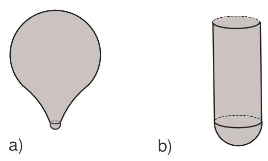
Figure 5.1. a) Curved truncation surface, b) problem domain for the boundary layer.

5.2. Other shapes of blunting.

We consider the case where the truncation surface of the blunted cuspidal domain $\Omega^{\varepsilon}$ is defined by

$$\Upsilon^{\varepsilon}=\big{\{}(y,z)\,:\,\big{(}\varepsilon^{-2}y,\varepsilon^{-2}(z-\varepsilon)\big{)}\in\Upsilon\big{\}}$$

where $\Upsilon\subset{\mathbb{R}}_{-}^{n}$ is a piecewise smooth surface which touches the half-space ${\mathbb{R}}_{+}^{n}$ at $\partial\omega\times\{0\}$, see Fig. 5.1, a). Then, the spectrum of the Steklov-Dirichlet problem composed of the equations (1.10), (1.11) and

$$u^{\varepsilon}(x)=0,\,x\in\Upsilon^{\varepsilon}$$

gets precisely the same properties as we established above for the domain (1.9) with the straight truncation surface. The only noteworthy modification in the proofs is related to the orthogonality condition (2.11) for the correction term $W$ in the asymptotic expansions near the cusp tip ${\mathcal{O}}$; these also appear in Section 4.4, where they provide the exponential decay of the boundary layer terms $Y_{\pm}$. In the case of a curved truncation surface as in Fig. 5.1, b), the boundary layer is to be found from the mixed boundary value problem

$$-\Delta_{\xi}Y_{\pm}(\xi)=0,\,\xi\in\Xi_{U},\ \ \ \ \partial_{\nu^{\prime}}Y_{\pm}(\xi)=0,\,\xi\in\Sigma,$$

(5.4) $$Y_{\pm}(\xi)=W_{\pm}(\xi^{\prime},1),\,\xi\in\Upsilon,$$

in the domain $\Xi_{U}$ which is bounded by the surfaces $\Sigma$ and $\Upsilon$ and contains the half-cylinder (4.25). The homogeneous problem (5.4) has a solution of the form

$${\mathcal{Y}}(\xi)=|\omega|^{-1}\xi_{n}+C_{\mathcal{Y}}+O(e^{-\beta_{\Xi}\xi_{n}})\ \ \mbox{as}\ \xi_{n}\to+\infty.$$

Then, the exponential decay of the solution $Y_{\pm}$ of (5.4) is supported by the orthogonality condition

(5.5) $$\int\limits_{\Upsilon}W_{\pm}(\xi^{\prime},1)\partial_{\nu}{\mathcal{Y}}(\xi)ds_{\xi}=0,$$

which replaces (2.11) everywhere. Note that in the case of a straight end $\omega^{\varepsilon}$ we have ${\mathcal{Y}}(\xi)=|\omega|^{-1}\xi_{n}$ so that formula (5.5) turns into (2.13).

5.3. Other boundary conditions at the end $\omega^{\varepsilon}$.

If the Dirichlet condition (1.12) is replaced by the Neumann condition

(5.6) $$\partial_{z}u^{\varepsilon}(x)=0\ ,\ \ x\in\omega^{\varepsilon},$$

the phenomena of blinking and gliding are preserved, but the relationship (4.4) is changed a bit, since the normal derivative of (4.3) vanishes at $z=\varepsilon$ provided

$$-2\tau_{0}(\lambda^{\flat})\ln\varepsilon=\Theta(\lambda^{\flat})+\vartheta(\lambda^{\flat})+\pi\ \ \ ({\rm mod}\,2\pi),$$

where

$$e^{i\vartheta_{n}(\lambda^{\flat})}=\frac{(n-3/2)-i\tau_{0}(\lambda^{\flat})}{(n-3/2)+i\tau_{0}(\lambda^{\flat})}.$$

The same formula and similar conclusions occur in the case of the Steklov condition

$$\partial_{z}u^{\varepsilon}(x)=\lambda^{\varepsilon}u^{\varepsilon}(x),\ \ x\in\omega^{\varepsilon};$$

the proofs require some minor modifications.

References

• [1] Birman, M.S.,. Solomyak, M.Z., Spectral theory of selfadjoint operators in Hilbert space. Leningrad Univ., Leningrad, 1980. English transl. Math. Appl. (Soviet Ser.), D. Reidel Publishing Co., Dordrecht, 1987.
• [2] Chesnel L., Claeys X., Nazarov S.A., A curious instability phenomenon for a rounded corner in presence of a negative material. Asymptotic Analysis 88 (2014), 43–74.
• [3] Chesnel L., Claeys X., Nazarov S.A., Oscillating behaviour of the spectrum for a plasmonic problem in a domain with a rounded corner. To appear in ESAIM: M2AN. doi: https://doi.org/10.1051/m2an/2016080
• [4] Kato, T., Perturbation Theory for linear operator edition, Grundlehren der Mathematischen Wissenschaften, Band 132, Springer, New York, 1976.
• [5] Kondratiev, V.A., Boundary value problems for elliptic problems in domains with conical or corner points. Trudy Moskov. Matem. Obshch. 16 (1967), 209–292. (English transl. Trans. Moscow Math. Soc. 16 (1967), 227–313.)
• [6] Kozlov, V.A., Nazarov, S.A., Waves and radiation conditions in a cuspidal sharpening of elastic bodies. J.Elasticity (2017).
• [7] Kozlov V.A., Maz’ya V.G., Rossmann J., Elliptic boundary value problems in domains with point singularities. Amer. Math. Soc., Providence, 1997.
• [8] Krylov, V.V., New type of vibration dampers utilising the effect of acoustic ’black holes’. Acta Acustica united with Acustica, 90 (2004) no.5, 830-837.
• [9] Ladyzhenskaya, O.A., Boundary value problems of mathematical physics. Springer Verlag , New York, 1985.
• [10] Mandelstam, L.I., Lectures on Optics, Relativity Theory, and Quantum Mechanics (in Russian), Akad. Nauk SSSR, Moscow, 1947.
• [11] Mazya, V. G., Poborchi, S. V., Imbedding and extension theorems for functions on non-Lipschitz domains. SPbGU publishing, 2006.
• [12] Mironov, M.A., Propagation of a flexural wave in a plate whose thickness decreases smoothly to zero in a finite interval, Soviet Physics-Acoustics 34 (1988), 318–319.
• [13] Mittra, R., Lee, S.W., Analytical Techniques in the Theory of Guided Waves, McMillan and Company, 1971.
• [14] Maz’ya V.G., Nazarov S.A., Plamenevskij, B.A., Asymptotic theory of elliptic boundary value problems in singularly perturbed domains. Vol. 1. Birkhäuser Verlag, Basel, 2000.
• [15] Maz’ya, V.G, Plamenevskii, B.A., Estimates in $L_{p}$ and Hölder classes and the Miranda-Agmon maximum principle for solutions of elliptic boundary value problems in domains with singular points on the boundary. Math. Nachr. 81 (1978), 25-82. (Engl. transl. Amer. Math. Soc. Transl. (Ser. 2) 123 (1984), 1-56 .)
• [16] Nazarov, S.A., Surface enthalpy, Dokl. Ross. Akad. Nauk. 421, no.1 (2008), 49–53 (English transl. Doklady Physics 53, no.7 (2008), 383–387).
• [17] Nazarov, S.A., Plamenevsky, B.A., Elliptic problems in domains with piecewise smooth boundaries. Walter de Gruyter, Berlin, New York, 1994.
• [18] Nazarov, S. A., Taskinen, J., On the spectrum of the Steklov problem in a domain with a peak. Vestnik St. Petersburg Univ. Math. 41 (2008), no. 1, 45–52.
• [19] Nazarov, S.A., Taskinen, J., Radiation conditions at the top of a rotational cusp in the theory of water-waves. Math.Model.Numer.Anal. 45,4 (2011), 947-979.
• [20] Nazarov, S.A., Taskinen, J., Spectral anomalies of the Robin Laplacian in non-Lipschitz domains. J. Math. Sci. Univ. Tokyo 20 (2013), 27–90.
• [21] Vishik, M.I., Lusternik, L.A., Regular degeneration and boundary layer for linear differential equations with small parameter (in Russian), Usp. Mat. Nauk 12, No. 5 (1957), 3–122.
• [22] Wilcox, C.H., Scattering Theory for Diffraction Gratings. Applied Mathematical Sciences Series, vol. 46. Springer, Berlin, 1997.