Peaks and cusps: anomalous thresholds and LHC physics

Abstract

The behavior of scattering amplitudes in the vicinity of a physical-region Landau singularity is considered. The impact on LHC processes is discussed.

1 Introduction

Resonances are normally observed as peaks in certain invariant mass distributions; however, a question arises: is a peak necessarily due to the presence of a resonance? Are there peaks produced by kinematic singularities?

Landau equations for a given Feynman integral are a set of kinematic constraints that are necessary for the appearance of a pole or branch point in the integrated function (as a function of external kinematics and masses). Landau equations admit many families of solutions which are naturally classified as leading Landau singularities (LLS), sub-leading Landau singularities (SLLS), sub-sub-leading (S²LLS) etc.

Leading Landau singularities have been studied mostly in the context of hadron spectroscopy [1] where, in order to establish an unambiguous strategy it is important to distinguish kinematic singularities from genuine resonances, i.e. poles of the ${\mathrm{S}}\,$-matrix. An example is ${\mathrm{B}}^{+}\to{\mathrm{B}}^{0}_{{\mathrm{s}}}\pi^{+}\pi^{0}$ via ${\mathrm{B}}{\overline{{\mathrm{K}}}}^{*}$ rescattering [2, 3].

As an example, a triangle singularity is a logarithmic branch point, which would produce an infinite reaction rate if it appears in the physical region. This never happens because at least one of the three particles must be unstable. The finite width, introduced by the complex-mass scheme [4, 5, 6], moves the singularity into the complex plane, and the differential reaction rate can have a finite peak due to the proximity of the singularity. Here, by complex plane we mean complex plane for Mandelstam invariants or complex hypersurface in the parametric representation of the corresponding diagram, i.e. no pinch singularity in Feynman parameter space.

The subject of Feynman amplitudes with variable momenta and non-zero masses has been studied by physicists since the 1950’s, e.g. the inelastic scattering ${}{{}{{{{{\mathrm{{{}{}{{{}{{}{{{{{\mathrm{{{}{}{{K}}\mspace{-0.6mu}}}}}}}}}}^{+}}\mspace{-0.6mu}}}}}}}}}+{}{{}{{{{{\mathrm{{{}{}{{p}}\mspace{-0.6mu}}}}}}}}}\to{}{{}{{{{{\mathrm{{{}{}{{{}{{}{{{{{\mathrm{{{}{}{}\mspace{-0.6mu}}}}}}}}}}^{+}}\mspace{-0.6mu}}}}}}}}}+{}{{}{{{{{\mathrm{{{}{}{{{}{{}{{{{{\mathrm{{{}{}{}\mspace{-0.6mu}}}}}}}}}}^{0}}\mspace{-0.6mu}}}}}}}}}+{}{{}{{{{{\mathrm{{{}{}{{p}}\mspace{-0.6mu}}}}}}}}}$ (see Figs.[1,2] of Ref. [7]). Meanwhile new mathematical methods involving Hodge structures and variations of Hodge structures have been developed. The use of these techniques to the study of amplitudes and Landau singularities in momentum space has been described in Refs. [8, 9]. A determination of the complete set of branch points of amplitudes in planar $N=4$ super-Yang-Mills theory directly from the amplituhedron, without resorting to any particular representation in terms of local Feynman integrals has been presented in Ref. [10].

However, in recent years, not much attention has been paid to the problem in the context of high energy physics, with the noticeable exception of the work by Boudjema and collaborators [11, 12, 13] (see also section 4.4 of Ref. [14], Ref. [15] and developments in the Golem95 project, e.g. Ref. [16]).

In this paper we analyze typical LHC processes looking for possible effects due to the presence of a leading Landau singularity, or anomalous threshold (hereafter AT). It should be stressed that by “cusp” we mean a cusp in some differential distribution (e.g. invariant mass or $p_{{\mathrm{T}}}$) and not cusp of a Landau variety .

In the rest of this paper we discuss the complications that arise in dealing with the singular part of a scattering amplitudes and the impact of anomalous thresholds on LHC physics. We begin in section 2 by reviewing briefly the definition of leading Landau singularities, illustrating the introduction of complex masses.

In section 3 – section 7 we describe LLS for two-, three-, $\dots$ six-point functions using the complex mass scheme discussed in subsection 2.1. In section 8 we include two-loop diagrams into our analysis. In section 9 we discuss special configurations leading to non-integrable LLS, even within the regularization introduced by complex masses. QED/QCD induced LLS, not to be mistaken for the infrared ones, are presented in subsection 4.1. In section 10 we discuss relatively simple examples of beyond-standard-model (BSM) LLS. In A – B technical details are presented.

2 Leading Landau singularities

Learning from the study of singularities of scattering amplitudes:

• For a given Feynman diagram there exists a discriminant

  $${\mathrm{D}}\left({p_{i}}\cdot{p_{j}},m^{2}_{i},\alpha_{i}\right),$$ (1)

  which is an homogeneous polynomial in the $\alpha_{i}$ and whose coefficients are linear in the ${p_{i}}\cdot{p_{j}}$  and $m^{2}_{i}$, such that the equations $\partial{\mathrm{D}}/\partial\alpha_{i}=0$ are equivalent to the usual Landau conditions for the existence of the singularity, as described in Ref. [18]. As it is well known, given any $m$ homogeneous polynomials in $m$ unknowns there exists a unique minimal homogeneous polynomial in the coefficients (${\mathrm{R}}$ the resultant) such that ${\mathrm{R}}=0$ is a necessary and sufficient condition for the existence of a solution to the system of equations (Landau-Nakanishi equations), distinct from the trivial solution $\alpha_{1}=\,\dots\,\alpha_{m}=0$ . Note that $\alpha_{i}\geq 0$ is required for the scattering to be physical (the so-called $+\,\alpha$ Landau surfaces, as opposite to “mixed-$\,\alpha$” solutions).

• The leading Landau singularity requires all of the$\alpha_{i}$’s to be non zero; the case where some of the parameters vanish can be interpreted as the leading singularity of a diagram obtained from the original one contracting the lines associated to the vanishing $\alpha$’s. Note that the definition used in Ref. [27] differs slightly from our conventional usage. Furthermore, for a given set of values $(p_{1},\,\dots\,,p_{{\mathrm{N}}})$ which lie on the given physical-region Landau singularity there exists only one unique set of values for the internal momenta which satisfy the Landau equations.

For the discussion of LL singularities there are three important theorems.

Theorem 2.1 (Coleman and Norton [28])

A Feynman amplitude has singularities on the physical boundary if and only if the relevant Feynman diagram can be interpreted as a picture of an energy- and momentum-conserving process occurring in space-time, with all internal particles real, on the mass shell, and moving forward in time. As a by-product, the Feynman parameter associated with an internal line is identified (within a proportionality factor) with the time the particle exists between collisions, divided by its mass.

Additional results can be found in Refs. [29, 30, 31, 32, 33, 34]. Other results can be found in Ref. [35], where it is stressed that the meaning of “physical boundary” in the Coleman-Norton theorem is as follows: consider the triangle of Figure 3, the unitary cut starts at $(m_{1}+m_{3})^{2}$ (right-hand branch cut); the physical boundary is just above the cut. To give an example, the original Peierls mechanism [36] gives singularities on the wrong sheet; the modified Peierls mechanism [37] gives the (triangular) singularity on the correct sheet but it has been shown that does not produce peaks in invariant-mass plots, the so-called Schmid theorem [35]. Nevertheless, in Ref. [38] it was argued that terms involving the singularity of a triangle diagram can in principle at least lead to observable effects in the differential cross section. Other counterexamples can be found in Ref. [39] and in Refs. [40, 41]. However, one should be aware that most of these papers limit their analysis to triangular singularities.

Theorem 2.2 (Kershaw [42])

The singular part of a scattering amplitude around its leading Landau singularity may be written as an algebraic product of the scattering amplitudes for each vertex of the corresponding Landau graph times a certain explicitly determined singularity factor which depends only on the type of singularity (triangle graph, box graph, etc.) and on the masses and spins of the internal particles.

It is worth noting that the consequences of the theorem have been reinterpreted by various authors in terms of multiple cuts on Feynman diagrams [43, 44, 45, 46, 47, 48, 49, 50].

Kershaw theorem is based on the fact that there always exists a finite polynomial in the scalar product of the external momenta such that ${\mathrm{P}}({p_{i}}\cdot{p_{j}})=0$ gives the location of the leading Landau singularity. The proof of this property is particularly simple for one-loop diagrams. Consider a scalar, one-loop, ${\mathrm{N}}$-point functions in ${\mathrm{d}}$ dimensions (${\mathrm{d}}=4-\varepsilon$): external momenta will be labelled as $p_{1},\,\dots\,p_{{\mathrm{N}}}$ and let us consider ${\cal P}_{{\mathrm{N}}}$ the set of the non-cyclic permutation of $\left(1,\,\dots\,{\mathrm{N}}\right)$ with the first entry fixed. Vectors $k_{i}$ are introduced according to the following convention:

• there are two elements, i.e. $\left(1,2,3\right)$ and $\left(1,3,2\right)$. We define

  $$\left(1,2,3\right) \to \quad k_{1}=p_{1},\;k_{2}=p_{2},$$

  $$\left(1,3,2\right) \to \quad k_{1}=p_{1},\;k_{2}=p_{3}.$$ (2)

• There are three elements and we define

  $$\left(1,2,3,4\right) \to \quad k_{1}=p_{1},\;k_{2}=p_{2},\;k_{3}=p_{3},$$

  $$\left(1,2,4,3\right) \to \quad k_{1}=p_{1},\;k_{2}=p_{2},\;k_{3}=p_{4},$$

  $$\left(1,3,2,4\right) \to \quad k_{1}=p_{1},\;k_{2}=p_{3},\;k_{3}=p_{2}.,$$ (3)

• There are twelve elements, etc.

With the notations of Ref. [51] we define a scalar integral as

$${\mathrm{S}}_{{\mathrm{d}}\,;\,{\mathrm{N}}}\left({\mathrm{w}}\right)=\frac{\mu^{\varepsilon}}{i\,\pi^{2}}\,\int\,d^{{\mathrm{d}}}q\,\frac{1}{\prod_{i=0,{\mathrm{N}}-1}\,[i]},\qquad[i]=\left(q+k_{0}+\,\cdots\,+k_{i}\right)^{2}+m^{2}_{i},$$ (4)

where $k_{0}=0$ and where ${\mathrm{w}}$ is an element of ${\cal P}_{{\mathrm{N}}}$. Furthermore $\mu$ is the ’t Hooft scale and $\varepsilon={\mathrm{d}}-4$. In this way we can characterize the whole set of ${\mathrm{N}}\,$-point functions contributing to a given amplitude and not just one specific diagram.

In parametric space we obtain

$${\mathrm{S}}_{{\mathrm{d}}\,{\mathrm{N}}}\left({\mathrm{w}}\right)=\left(\frac{\mu^{2}}{\pi}\right)^{2-{\mathrm{d}}/2}\,\Gamma({\mathrm{N}}-\frac{{\mathrm{d}}}{2})\,[{\mathrm{N}}]_{{\mathrm{d}}}({\mathrm{w}}),$$ (5)

where from the triangle to the hexagon we will use the following notations: $[3]\equiv{\mathrm{C}},\,\dots\,[7]\equiv{\mathrm{G}}$. We have

$$[{\mathrm{N}}]_{{\mathrm{d}}}(w)=\int\,dS_{{\mathrm{N}}-1}\,{\mathrm{V}}^{{\mathrm{d}}/2-{\mathrm{N}}}_{{\mathrm{N}}}({\mathrm{w}}),$$ (6)

$${\mathrm{V}}_{{\mathrm{N}}}(w)=x^{t}\,{\mathrm{H}}_{{\mathrm{N}}}({\mathrm{w}})\,x+2\,{\mathrm{K}}^{t}_{{\mathrm{N}}}({\mathrm{w}})\,x+{\mathrm{L}}_{{\mathrm{N}}}(w),\quad X_{{\mathrm{N}}}(w)=-{\mathrm{K}}^{t}_{{\mathrm{N}}}({\mathrm{w}})\,{\mathrm{H}}^{-1}_{{\mathrm{N}}}({\mathrm{w}}),$$ (7)

$$\Delta_{{\mathrm{N}}}(w)={\mathrm{L}}_{{\mathrm{N}}}({\mathrm{w}})-{\mathrm{K}}^{t}_{{\mathrm{N}}}({\mathrm{w}})\,{\mathrm{H}}^{-1}_{{\mathrm{N}}}({\mathrm{w}})\,{\mathrm{K}}_{{\mathrm{N}}}({\mathrm{w}}),$$ (8)

where ${\mathrm{H}}_{ij}=-\,{k_{i}}\cdot{k_{j}}$; ${\mathrm{G}}_{{\mathrm{N}}}=\mathrm{det}\,{\mathrm{H}}_{{\mathrm{N}}}$ is the Gram determinant associated with the ${\mathrm{N}}\,$-point function of argument ${\mathrm{w}}\in{\cal P}_{{\mathrm{N}}}$. Furthermore, ${\mathrm{K}}_{i}=-1/2\,(m^{2}_{i}-m^{2}_{i+1}-k^{2}_{i}-2\,\sum_{j=1,i-1}\,{k_{j}}\cdot{k_{i}})$, ${\mathrm{L}}=m^{2}_{1}$ and

$$\int\,dS_{{\mathrm{N}}-1}=\int_{0}^{1}dx_{1}\,\int_{0}^{x_{1}}dx_{2}\,\dots\,\int_{0}^{x_{{\mathrm{N}}-2}}dx_{{\mathrm{N}}-1}\,\,.$$ (9)

Let ${\mathrm{M}}_{{\mathrm{N}}}$ be the ${\mathrm{N}}\,\times\,{\mathrm{N}}$ matrix

$${\mathrm{M}}_{{\mathrm{N}}}=\left(\begin{array}[]{cc}{\mathrm{H}}_{{\mathrm{N}}}&{\mathrm{K}}_{{\mathrm{N}}}\\ {\mathrm{K}}^{t}_{{\mathrm{N}}}&{\mathrm{L}}_{{\mathrm{N}}}\\ \end{array}\right)$$

Then one can easily prove that

$$\Delta_{{\mathrm{N}}}({\mathrm{w}})=\frac{{\mathrm{C}}_{{\mathrm{N}}}({\mathrm{w}})}{{\mathrm{G}}_{{\mathrm{N}}}({\mathrm{w}})}\,,\qquad X^{i}_{{\mathrm{N}}}=\frac{\mathrm{det}\,{\mathrm{M}}_{(i\,,\,{\mathrm{N}})}}{{\mathrm{G}}_{{\mathrm{N}}}}\,,$$ (10)

where ${\mathrm{C}}_{{\mathrm{N}}}=\mathrm{det}\,{\mathrm{M}}_{{\mathrm{N}}}$ is the so-called modified Cayley determinant [52, 53] of the diagram  and we can write

$${\mathrm{V}}_{{\mathrm{N}}}=\left(x-X_{{\mathrm{N}}}\right)^{t}\,{\mathrm{H}}_{{\mathrm{N}}}\,\left(x-X_{{\mathrm{N}}}\right)+\Delta_{{\mathrm{N}}}=y^{t}\,{\mathrm{M}}_{{\mathrm{N}}}\,y\,,$$ (11)

where $y^{t}=(x^{t}\,,\,1)$.

Theorem 2.3 (Ferroglia et al.  [51]; Goria and Passarino [55])

It is easily seen  that $\Delta_{{\mathrm{N}}}=0$ induces a pinch [57, 58, 59] on the integration contour at the point $x=X_{{\mathrm{N}}}$; therefore, if

$$\Delta_{{\mathrm{N}}}=0,\qquad 0<X_{{\mathrm{N}},{\mathrm{N}}-1}<\,\dots\,<X_{{\mathrm{N}},1}<1,$$ (12)

we have the leading singularity (from Eq.(11) we derive that it represents a singular point of multiplicity two). Leading singularities of diagrams obtained by shrinking one (or more) line of the original diagram to a point give the sub-leading singularities.

In the Cayley language the Landau equations for a general case can be written as follows. Consider the integral

$${\mathrm{I}}=\int_{{\mathrm{D}}}\,\prod_{i=1}^{n}\,dx_{i}\,{\mathrm{V}}^{-\mu}_{{\mathrm{N}},n}\left(x_{1}\,\dots\,x_{n}\,;\,w_{1}\,\dots\,w_{k}\right)\,,$$ (13)

where ${\mathrm{V}}$ is a multivariate polynomial of degree ${\mathrm{N}}$ and an algebraic function of $k\,$-parameters $w_{1}\,\dots\,w_{k}$. Therefore ${\mathrm{V}}\in\mathbb{C}\left[x\,,\,w\right]$. ${\mathrm{D}}$ is the domain of integration. ${\mathrm{V}}_{{\mathrm{N}},n}=0$ is the locus of the singularities of the integrand; let $\mathcal{B}_{j}\left(x\,,\,w\right)$, $j=1,\,\dots\,,d$ be the set representing the boundary of ${\mathrm{D}}$.

Proposition 2.4

The necessary conditions for the leading singularities to occur when the hypercontour is pinched between the surfaces of singularity or meets a boundary variety are

• $\exists\;\;\alpha_{i}\,,\,\beta$, not all equal to zero and such that at the point $w_{k}=w^{0}_{k}$ and $x_{k}=x^{0}_{k}$ we have $\beta\,{\mathrm{V}}_{{\mathrm{N}},n}=0$ and

$$\alpha_{i}\,\mathcal{B}_{i}\left(x_{i}\,,\,w_{i}\right)=0,\qquad i=1,\,\dots\,,d\,,$$

$$\frac{\partial}{\partial x_{i}}\,\left[\sum_{i}\,\alpha_{i}\,\mathcal{B}_{i}\left(x\,,\,w\right)+\beta\,{\mathrm{V}}_{{\mathrm{N}},n}\left(x\,,\,w\right)\right]=0,\qquad i=1,\,\dots\,,n\,\,.$$ (14)

If ${\mathrm{D}}$ is a $n\,$-dimensional hypercube and

$${\mathrm{V}}_{{\mathrm{N}}\,,\,n}=\sum_{i=0}^{{\mathrm{N}}}\,{\mathrm{V}}^{i}_{n}\,,\qquad{\mathrm{V}}^{i}_{n}=\sum_{0\leq i_{1}=\,\cdots\,i_{n}\leq i}\,a^{i}_{i_{1}\,\dots\,i_{n}}\,x^{i_{1}}_{1}\,\cdots\,x^{i_{n}}_{n}\,,$$ (15)

where the ${\mathrm{V}}^{i}_{n}$ are homogeneous polynomials and ${\mathrm{V}}_{{\mathrm{N}}\,,\,n}$ is a generic polynomial in the ring of polynomials of degree ${\mathrm{N}}$, it is convenient to determine the $({\mathrm{N}}-1)^{n}$ n-tuples $X^{i}_{1}\,\dots\,X^{i}_{n}$ such that

$${\mathrm{V}}_{{\mathrm{N}}\,,\,n}\left(x_{1}-X^{i}_{1}\,\dots\,x_{n}-X^{i}_{n}\right)=\Delta+\sum_{i=2}^{{\mathrm{N}}}\,{\mathrm{V}}^{i}_{n}\left(x_{1}-X^{i}_{1}\,\dots\,x_{n}-X^{i}_{n}\right),\quad i=1\,\dots\,({\mathrm{N}}-1)^{n}\,,$$ (16)

so that the solutions of $\Delta\left(w_{1}\,\dots\,w_{k}\right)=0$, are the potential (leading) pinch singularities if $X^{i}_{j}\in\mathbb{R}\,,\;\;0<X^{i}_{j}<1\;\;\forall j$. For ${\mathrm{V}}^{2}_{n}=\,\dots\,={\mathrm{V}}^{k}_{n}=0$ the singular point will have multiplicity $k+1$.

To summarize: a general understanding of the behavior of Feynman amplitudes may be obtained by analogy with the behavior of a function $f$ of a single complex variable ${\mathrm{z}}$, defined as a contour integral with respect to a second variable $s$ of a function $g$ analytic in ${\mathrm{z}}$ and $s$. The singularities of $f({\mathrm{z}})$ arise for values of ${\mathrm{z}}$ for which two singularities of $g({\mathrm{z}},s)$ coincide in the $s$ plane, trapping the contour of integration. A general point on a Landau singularity corresponds to the occurrence in the integration space of the analog of this mechanism for functions of several complex variables. The extension to more than one external variables and the situations where a pinch may become harmless (e.g. falling off the end of the contour) are discussed in chapter 2.1 of Ref. [57]; the extension to multiple integrals can also be found there and in Eq.(14).

There also exist “second-type” (so-called non-Landau) singularities (see for example Ref. [57]). These arise in Feynman loop integrals as pinch singularities at infinite loop momentum and will not be analyzed in this work.

More details on Landau singularities

For more details from the point of view of algebraic geometry see Refs. [53, 17]. Landau equations in the context of the theory of asymptotic operation have been discussed in Ref. [60]. Finally, solutions to the Landau conditions, corresponding to kinematic configurations where the modified Cayley determinant vanishes, are called singularities of the first type (singularities of the first type comprise all solutions to the Landau conditions for finite values of loop momentum); for a geometric interpretation in terms of volumes of polytopes see Ref. [61]. For an interpretation in terms of projective geometry and momentum twistors see Ref. [62]. For the analyticity properties of amplitudes in theories with nonlocal vertices of the type occurring in string field theory see Ref. [63]. For Landau diagrams in theories with gravity duals see Ref. [64]. Furthermore, for amplitudes of generalized polylogarithm type there should be a close connection between symbol entries and solutions of the Landau equations [64]. The most recent developments deal with massless theories which is of no help here since, in our case, at least one internal line must have nonzero mass.

Another description of the AT is as follows: $3$ and higher point functions can be cut im more that two pieces; putting all propagators on-shell corresponds to $\alpha_{i}\not=0$ at the level of the Landau equations, i.e. ATs go beyond the concept of unitarity cuts [65, 66, 7]. For an alternative proof of cutting rules in quantum field theories see Ref. [67].

Vanishing Cayley determinants have been mentioned in the literature but, usually, this case has not been considered in detail since “the exceptional case with a vanishing modified Cayley determinant hardly appears in applications”, see Refs. [68, 54]; however, reduction of tensor integrals for small Gram determinant and/or small modified Cayley determinant have been discussed in Ref. [69].

The expansion of Feynman integrals around their AT is easy to derive analytically and only requires Mellin-Barnes and sector decomposition techniques as explained in Ref. [51]. Examples of leading behavior (details are given in B) are: for the vertex ${\mathrm{C}}_{0}\sim\ln\,\Delta_{3}$; for the box ${\mathrm{D}}_{0}\sim\Delta^{-1/2}_{4}$; for the pentagon ${\mathrm{E}}_{0}\sim\Delta^{-1}_{5}$ and no singularity for the hexagon ${\mathrm{F}}_{0}$ in $4\,$dimensions [57]; e.g. $\;\mathop{\mathrm{Im}}\nolimits\,{\mathrm{C}}_{0}$ has a logarithmic singularity, $\;\mathop{\mathrm{Re}}\nolimits\,{\mathrm{C}}_{0}$ has a discontinuity. $\Delta_{n}$ is analytic in the immediate vicinity of the given singularity and singular on it. Of course, we can add any function, analytic in the neighborhood of the singularity. The general result can be summarized as follows: let ${\mathrm{L}}$ be the number of internal lines in the Feynman diagram under consideration and $\nu$ the number of loops; define $\rho=2\,\nu-1/2\,({\mathrm{L}}+1)$, the leading behavior of the diagram is given by (special cases are discussed in B)

$$\Delta^{\rho}_{{\mathrm{L}}}\;\;\mbox{for}\;\;\rho<0\,,\quad\Delta^{k+1/2}_{{\mathrm{L}}}\;\;\mbox{for}\;\;\rho=k+\frac{1}{2}\,,\quad\Delta^{k}_{{\mathrm{L}}}\,\ln\Delta_{{\mathrm{L}}}\;\;\mbox{for}\;\;\rho=k\,,\quad k\in\mathbb{Z}^{*}\,\,.$$ (17)

Therefore for ${\mathrm{L}}=2\,(2\,\nu+n)-1$ and $n\in\mathbb{Z}^{+}$ the AT is a pole of order $n$ for the amplitude, e.g. a simple pole for the one-loop pentagon, for two-loop diagrams with $9$ propagators etc. In all other cases it is a branch point.

• Any one-loop diagram is specified by

  • ${\mathrm{H}}_{{\mathrm{N}}}$, a $({\mathrm{N}}-1)\,\times\,({\mathrm{N}}-1)$ matrix whose determinant is the Gram determinant.

  • The set $\{X_{1}\,,\,\dots\,,\,X_{{\mathrm{N}}-1}\}=\mathrm{X}_{{\mathrm{N}}}$; we will denote by $\mathrm{X}^{{\mbox{\scriptsize{ord}}}}_{{\mathrm{N}}}$ the set $\{(X_{1},\,\dots\,,X_{{\mathrm{N}}-1})\in\mathbb{R}^{{\mathrm{N}}+1}\mid 0<X_{{\mathrm{N}}-1}<\,\dots\,X_{1}<1\}$.

  • The Bernstein-Sato-Tkachov [70, 71, 72] factor $\Delta_{{\mathrm{N}}}$ defined in Eqs.(8)–(10). The Bernstein theorem [70] states that for any polynomial in $\mathbb{C}[x]$ there exists a non-zero polynomial $b(s)\in\mathbb{C}[s]$ (Berstein-Sato polynomial [70, 71]) and a differential operator ${\mathrm{P}}(s)\in D_{n}(s)$ such that ${\mathrm{P}}(s)\,\cdot\,f^{s+1}=b(s)\,f^{s}$. For one-loop diagrams $\Delta_{{\mathrm{N}}}$ is the explicit form of $b$, as shown in Ref. [72].

  • The set of generalized Mandelstam invariants, $\mathrm{I}$; we will denote by $\mathrm{I}_{{\mbox{\scriptsize{phys}}}}$ a set of invariants internal to the physical region .

• Assume that all masses are real ($\{\Gamma\}=0$), the physical-region LLS (or physical-region anomalous threshold) is given by

  $$\Delta_{{\mathrm{N}}}\Bigr{|}_{\{\Gamma\}=0}=0\,,\quad\mathrm{X}_{{\mathrm{N}}}=\mathrm{X}^{{\mbox{\scriptsize{ord}}}}_{{\mathrm{N}}}\,,\quad\{\mathrm{I}\}=\{\mathrm{I}\}_{{\mbox{\scriptsize{phys}}}}\,\,.$$ (18)

  There are cases where the first two conditions are satisfied but Mandelstam invariants are moved to their complex plane. Nevertheless, their real part can be inside the physical region with a tiny imaginary part; therefore they can be very close to the boundary. When internal masses are made complex, i.e. $m^{2}_{i}\to m^{2}_{i}-i\,\Gamma_{i}\,m_{i}$, singularities move into the complex $x\,$-space. We are nevertheless interested in the following configurations:

  $$\begin{array}[]{ll}\mathop{\mathrm{Re}}\nolimits\,\Delta_{{\mathrm{N}}}\approx\Delta_{{\mathrm{N}}}\Bigr{|}_{\{\Gamma\}=0}\approx 0\,,&\quad\mathop{\mathrm{Im}}\nolimits\,\Delta_{{\mathrm{N}}}\ll 1\,,\\ &\\ \{\mathop{\mathrm{Re}}\nolimits\,X_{i}\}=\{\mathop{\mathrm{Re}}\nolimits\,X_{i}\}^{{\mbox{\scriptsize{ord}}}}\,,&\quad\mathop{\mathrm{Im}}\nolimits\,X_{i}\ll 1\,,\end{array}$$

  with $\{\mathrm{I}\}=\{\mathrm{I}\}_{{\mbox{\scriptsize{phys}}}}$. The introduction of complex masses regularizes the singularity since, in general, $\mathop{\mathrm{Im}}\nolimits\,\Delta_{{\mathrm{N}}}\not=0$; however another special configuration is possible:

• They are defined by

  $$\mathop{\mathrm{Re}}\nolimits\,\Delta_{{\mathrm{N}}}=\mathop{\mathrm{Im}}\nolimits\,\Delta_{{\mathrm{N}}}=0\,,$$ (19)

  and we look for a set of “real” invariants that satisfy Eq.(19), possibly within the physical region and with $\{\mathop{\mathrm{Re}}\nolimits\,X_{i}\}=\{\mathop{\mathrm{Re}}\nolimits\,X_{i}\}^{{\mbox{\scriptsize{ord}}}}$. The effect of these zeros can be seen by considering a simple example:

  $${\mathrm{F}}(y\,,\,{\mathrm{z}})=\int_{-1}^{+1}dx\,\Bigl{[}(x+i\,y)^{2}-{\mathrm{z}}^{2}\Bigr{]}^{-1}\,,$$ (20)

  where $y\in\mathbb{R}$ and ${\mathrm{z}}\in\mathbb{C}$. We derive

  $${\mathrm{F}}(y\,,\,{\mathrm{z}}) = \frac{1}{2\,{\mathrm{z}}}\,\Bigl{\{}\ln\Bigl{[}({\mathrm{z}}-1)^{2}+y^{2}\Bigr{]}-\ln\Bigl{[}({\mathrm{z}}+1)^{2}+y^{2}\Bigr{]}+\eta({\mathrm{z}}-1\,,\,{\mathrm{z}}-1)\Bigr{\}}$$ (21)

  $$= \frac{1}{2\,{\mathrm{z}}}\,\Bigl{[}\ln\frac{{\mathrm{z}}-1-i\,y}{{\mathrm{z}}+1-i\,y}-\ln\frac{{\mathrm{z}}+1+i\,y}{{\mathrm{z}}-1+i\,y}\Bigr{]}\,,$$

  where $\eta$ is the ’t Hooft-Veltman eta function [73] and the $\ln{\mathrm{v}}$ denotes the principal branch, $-\pi<\mbox{arg}({\mathrm{v}})\leq+\pi$. If ${\mathrm{z}}=\alpha+i\,\beta$ with $-1\leq\alpha\leq+1$ and $\beta\geq 0$ we derive

  $${\mathrm{F}}(0\,,\,{\mathrm{z}})\sim\frac{i\,\pi}{{\mathrm{z}}}\,,\qquad\mbox{for}\;\;{\mathrm{z}}\to 0\,,$$ (22)

  showing a pinch singularity for ${\mathrm{z}}=0$. When we set ${\mathrm{z}}=0$ with $y\not=0$ we obtain

  $${\mathrm{F}}(y\,,\,0)=-\frac{2}{1+y^{2}}\,,$$ (23)

  without a pinch, i.e. one double pole of the integrand at $x=-i\,y$ instead of two simple poles at $x=\pm{\mathrm{z}}$. In general, let us consider

  $${\mathrm{F}}({\mathrm{z}}_{1}\,,\,{\mathrm{z}}_{2})=\int_{-1}^{+1}dx\,\Bigl{[}(x-{\mathrm{z}}_{1})^{2}-{\mathrm{z}}^{2}_{2}\Bigr{]}^{-1}\,,$$ (24)

  where ${\mathrm{z}}_{1,2}$ depend on real external parameters, $s_{1}\,,\,\dots\,,\,s_{n}$. Let $\Sigma$ be the hypersurface in $s\,$-space where ${\mathrm{z}}_{2}=0$; furthermore, let $\Pi_{+}$ be the hypersurface where $\mathop{\mathrm{Im}}\nolimits{\mathrm{z}}_{1}=0$ and $-1\leq\mathop{\mathrm{Re}}\nolimits{\mathrm{z}}_{1}\leq+1$. If we follow a path on $\Pi_{+}$ and approach $\Sigma$ a pinch will appear; starting with a point in $\Sigma$ and not in $\Pi_{+}$ and following any path on $\Sigma$ will not give a pinch singularity.

  To illustrate the behavior of ${\mathrm{F}}(y\,,\,{\mathrm{z}})$ we fix ${\mathrm{z}}=0.9+i\,10^{-3}$ and scale it with a factor $\lambda$, showing ${\mathrm{F}}(y\,,\,\lambda\,{\mathrm{z}})$ as a function of $\lambda$ for $y=0,10^{-6},10^{-5}$. The result is shown in Figure 1; for $y=0$ the $1/{\mathrm{z}}$ behavior in the imaginary part is evident. With small $y$ there is no pole but a discontinuity (a large gap) is present, corresponding to a value of $\lambda$ where the imaginary part of the first logarithm in Eq.(21) changes sign.

  

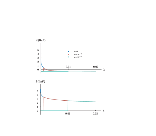
  Figure 1: Real and imaginary part of ${\mathrm{L}}({\mathrm{F}})$ where ${\mathrm{F}}$ is given in Eq.(20) and ${\mathrm{L}}$ is the log-modulus function [74] defined in Eq.(40).

A more detailed discussion concerning boxes and pentagons will be given in section 9.

• As long as $\mathop{\mathrm{Im}}\nolimits\,X_{i}\not=0$ there is no singularity, even if $\{\mathop{\mathrm{Re}}\nolimits\,X_{i}\}=\{\mathop{\mathrm{Re}}\nolimits\,X_{i}\}^{{\mbox{\scriptsize{ord}}}}$. In general the introduction of complex masses causes the singularity to be removed rather far from the real axis, i.e. the integral

  $$[{\mathrm{N}}]_{n}(w) = \int\,dS^{\gamma}_{{\mathrm{N}}-1}\,{\mathrm{V}}^{n/2-{\mathrm{N}}}_{{\mathrm{N}}}({\mathrm{w}})\,,$$

  $$\int\,dS^{\gamma}_{{\mathrm{N}}-1} = \int_{0\,\gamma_{1}}^{1}dx_{1}\,\int_{0\,\gamma_{2}}^{x_{1}}dx_{2}\,\dots\,\int_{0\,\gamma_{{\mathrm{N}}-1}}^{x_{{\mathrm{N}}-2}}dx_{{\mathrm{N}}-1}\,,$$ (25)

  is regular if the paths $\gamma_{i}$, connecting $0$ and $x_{i-1}$ lie on the real axis. This indicates a branch point of the integral that is not present on the physical sheet but only becomes apparent after suitable analytic continuation away from the physical contour. However, there are circumstances where the singularity can be shifted very near (or even inside) the physical region defined by $\{\mathop{\mathrm{Re}}\nolimits\,X_{i}\}=\{\mathop{\mathrm{Re}}\nolimits\,X_{i}\}^{{\mbox{\scriptsize{ord}}}}$, with $\{\mathop{\mathrm{Im}}\nolimits\,X_{i}\}=0$ and $\{\mathrm{I}\}=\{\mathrm{I}\}_{{\mbox{\scriptsize{phys}}}}$. In this case we will have the so-called Peierls or Brayshaw singularities [75, 76]. The scattering diagram generating the Brayshaw singularity is shown in Figure 2 where the blobs refer to off-shell scattering amplitudes and $A^{\prime},B^{\prime}$ are at threshold while $X$ is a resonance. Consider the $s\,$-plane for the $X{-}A$ scattering, the Peierls singularity is a special case occurring at $s=2\,(m^{2}_{X}+m^{2}_{A})-m^{2}_{B}$.

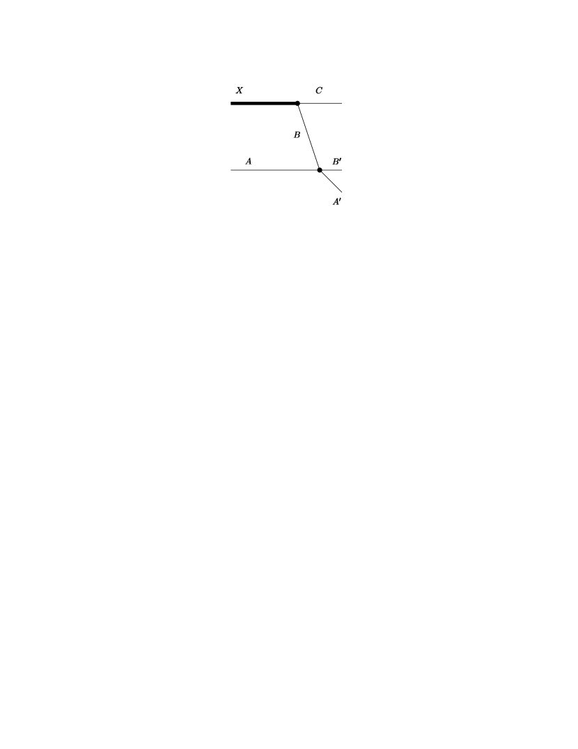
Figure 2: Diagram which generates the Brayshaw singularity [75, 76].

From Coleman-Norton theorem 2.1 and Kershaw theorem 2.2 we immediately realize that a physical-region singularity requires a theory with a hierarchy of heavy masses. Furthermore identical masses in a vertex must be avoided, e.g. $X$ and $C$ in Figure 2 cannot have the same mass; if we stay within the standard model this means that $B$ cannot be neutral, a ${}{{}{{{{{\mathrm{{{}{}{{Z}}\mspace{-0.6mu}}}}}}}}}$ or a ${}{{}{{{{{\mathrm{{{}{}{{H}}\mspace{-0.6mu}}}}}}}}}$ boson. Therefore we are limited to consider only two heavy particles, the ${}{{}{{{{{\mathrm{{{}{}{{t}}\mspace{-0.6mu}}}}}}}}}\,$-quark and the ${}{{}{{{{{\mathrm{{{}{}{{W}}\mspace{-0.6mu}}}}}}}}}\,$-boson. Furthermore, anomalous thresholds in the standard model (SM) prefer the so-called “off-shell” region, e.g. ${}{{}{{{{{\mathrm{{{}{}{{g}}\mspace{-0.6mu}}}}}}}}}{}{{}{{{{{\mathrm{{{}{}{{g}}\mspace{-0.6mu}}}}}}}}}$ producing an off-shell Higgs (with a virtuality greater that $2\,m_{{}{{}{{{{{\mathrm{{{}{}{{t}}\mspace{-0.6mu}}}}}}}}}}$) subsequently “decaying” into four fermions, see Refs. [77, 78]. The situation changes when we consider BSM models as we will discuss later.

2.1 Complex masses

The so-called “complex-mass scheme” has been introduced and discussed (in modern times) in Refs. [4, 5, 79, 6] (for an introduction before the advent of gauge theories see Ref. [80]; analiticity in the complex mass shell has been discussed in Ref. [81] ). An amplitude with unstable (internal) particles can be regarded as an analytic continuation of the amplitude defined by Feynman prescription.

One should remember that unstable states lie in a natural extension of the usual Hilbert space that corresponds to the second sheet of the ${\mathrm{S}}\,$-matrix ; for instance we will have to take the logarithm of ${\mathrm{z}}={\mathrm{z}}_{{\mathrm{R}}}+i\,{\mathrm{z}}_{{\mathrm{I}}}$, where ${\mathrm{z}}$ is the polynomial occurring in the calculation of a given Feynman diagram and where, in the limit of zero widths, we have ${\mathrm{z}}={\mathrm{z}}_{0}-i\,0$. The analytic continuation requires a new definition [82], i.e. the first Riemann sheet for all quadrants but the second where the function is defined in the second Riemann sheet:

$$\ln^{-}({\mathrm{z}}_{{\mathrm{R}}}+i\,{\mathrm{z}}_{{\mathrm{I}}}\,,\,{\mathrm{z}}_{0}-i\,0)=\ln(z_{{\mathrm{R}}}+i\,{\mathrm{z}}_{{\mathrm{I}}})-2\,i\,\pi\,\theta(-{\mathrm{z}}_{0})\,\theta({\mathrm{z}}_{{\mathrm{I}}})\,\,.$$ (26)

It is easily seen that, as far as Feynman diagrams are concerned, $\ln^{-}({\mathrm{z}})$ and $\ln({\mathrm{z}})$ coincide when the internal masses are made complex while Mandelstam invariants remain real.

The numerical evaluation of logarithms of complex quantities, when needed, is better performed by using

$$\ln x=x\,{\mathrm{R}}_{{\mathrm{c}}}\left(\frac{1}{4}\,x^{2}\,,\,x\right)\,,\qquad\arctan x=x\,{\mathrm{R}}_{{\mathrm{c}}}\left(1\,,\,1+x^{2}\right)\,,$$ (27)

where ${\mathrm{R}}_{{\mathrm{c}}}$ is one of the Carlson elliptic integrals [83].

In the following sections we will analyze the presence of regularized ATs for bubbles, triangles, boxes etc. and study their impact on physical observables; it should be emphasised that the presence of ATs depends on the structure of denominators of specific Feynman diagrams  but their numerical impact on the full amplitude also depends on numerators. In this regard, we are assuming that the singularity spectrum of the ${\mathrm{S}}\,$-matrix is confined to the union of the singularity spectra of the Feynman integrals, and we proceed to construct the singularity spectra of the Feynman integrals. Therefore, the scattering amplitude appears as the sum of infinitely many diagrams of increasing complexity and each diagram in principle can be completely investigated. In principle there is no reason for the ${\mathrm{S}}\,$-matrix to be the sum of the diagrams but we work under the assumption that the diagrams represent the local behavior of the amplitude and that the whole picture can be recovered by gluing together all these local behaviors. For an interpretation of the Landau singularities as macroscopic causality see Refs. [84, 85].

Furthermore, at the amplitude level, a given branch cut is generically shared by several integrals while the leading singularities receive contributions from a single integral . An additional comment concerns the difference between the Feynman diagram approach and the ${\mathrm{S}}\,$-matrix theory [88]. Feynman integrals can be analytically continued around a Landau singularity: as a consequence Feynman diagram integrals are clearly singular only on the Landau surfaces obtained from the so-called $+\,\alpha$ Landau equations [89]. In ${\mathrm{S}}\,$-matrix theory there is, a-priori, no $i\,\epsilon$ prescription (unless it is adopted as an additional postulate).

It should be emphasized that a complete numerical study of different processes falls outside the scope of this paper where we limited our analysis to the evaluation of the anomalous part of the amplitudes. Furthermore, we have not analyzed the impact of parton distribution functions but the general rule is that, given an amplitude (squared), increasing the number of integrations decreases the effect.

3 Bubble diagrams

The whole procedure can be understood in terms of a simple example, the generalized bubble integral,

$${\mathrm{B}}_{0}(\alpha)=\int_{0}^{1}dx\chi^{-\alpha}\,,\qquad\chi=s\,x^{2}+(m^{2}_{2}-m^{2}_{1}-s)\,x+m^{2}_{1}\,\,.$$ (28)

We introduce complex masses, $m^{2}_{i}\to m^{2}_{i}-i\,\Gamma_{i}\,m_{i}$, and derive

$$\chi=s\,(x-X)^{2}+\Delta_{2}\,,$$ (29)

where we have introduced

$$X=\frac{1}{2}\,\left(1+\frac{m^{2}_{1}-m^{2}_{2}}{2}\right)-\frac{i}{2}\,\frac{\Gamma_{-}}{s}\,,\quad\Delta_{2}=\lambda(s\,,\,m^{2}_{1}\,,\,m^{2}_{2})-\Gamma^{2}_{-}+2\,i\,\Bigl{[}\Gamma_{+}\,s-\Gamma_{-}\,(m^{2}_{1}-m^{2}_{2})\Bigr{]}\,,$$ (30)

where $\Gamma_{\pm}=\Gamma_{1}\,m_{1}\pm\Gamma_{2}\,m_{2}$ and where $\lambda$ is the Källen lambda function. With real masses the integral is singular when $0<X<1$ and $\lambda=0$, i.e. $s=(m_{1}\pm m_{2})^{2}$ which are the so-called normal and pseudo threshold. We obtain

$${\mathrm{B}}_{0}(\alpha)=\frac{\Gamma(\alpha-1/2)}{\Gamma(\alpha)}\,(\frac{\pi}{s})^{1/2}\,\Delta^{1/2-\alpha}_{2}+\quad\mbox{reg. terms}\,,$$ (31)

where $\Gamma$ is the Euler gamma function. Furthermore, at the normal threshold (the leading Landau singularity for the bubble) the condition $0<X<1$ is always satisfied. With complex masses there is no singularity but for

$$s=\frac{\Gamma_{1}\,m_{1}-\Gamma_{2}\,m_{2}}{\Gamma_{1}\,m_{1}+\Gamma_{2}\,m^{2}}\,(m^{2}_{1}-m^{2}_{2})\,,$$ (32)

we have the Peierls zero ($\mathop{\mathrm{Re}}\nolimits\,\Delta_{2}=\mathop{\mathrm{Im}}\nolimits\,\Delta_{2}=0$) if

$$4\,m^{2}_{1}\,m^{2}_{2}\,(m^{2}_{1}-m^{2}_{2})\,(\Gamma^{2}_{2}-\Gamma^{2}_{1})=(m^{2}_{1}\,\Gamma^{2}_{1}-m^{2}_{2}\,\Gamma^{2}_{2})^{2}\,\,.$$ (33)

To show the numerical effect we select $m_{1}=100~{}\text{GeV}$, $m_{2}=10~{}\text{GeV}$ and $\Gamma_{1}=100~{}\text{MeV}$. Deriving $\Gamma_{2}$ and $s=s_{*}$ from Eq.(33) we find $\sqrt{s_{{\mathrm{P}}{\mathrm{T}}}}-\sqrt{s_{*}}=112.5~{}\text{MeV}$, where the pseudo-threshold is at $90\,~{}\text{GeV}$. Numerical results are shown in Tab. 1 where it can be seen that $\mathop{\mathrm{Im}}\nolimits\,X$ is always negative, $\mathop{\mathrm{Re}}\nolimits\,X$ decreases with $s$ (but $\mathop{\mathrm{Re}}\nolimits\,X>1$ at the pseudo-threshold), there is a cusp at the normal threshold and no special enhancement at $\sqrt{s_{*}}$.

$\sqrt{s}[~{}\text{GeV}]$	$\mathop{\mathrm{Re}}\nolimits{\mathrm{B}}_{0}(1)$	$\mathop{\mathrm{Im}}\nolimits{\mathrm{B}}_{0}(1)$	$\mathop{\mathrm{Re}}\nolimits\Delta_{2}$	$\mathop{\mathrm{Im}}\nolimits\Delta_{2}$	$\mathop{\mathrm{Re}}\nolimits X$	$\mathop{\mathrm{Im}}\nolimits X$
$80$	$0.78746\,10^{-3}$	$0.34494\,10^{-5}$	$-0.59143\,10^{-1}$	$0.22827\,10^{-3}$	$1.2734$	$-0.7031\,10^{-3}$
$\sqrt{s_{*}}$	$0.99996\,10^{-3}$	$0.54997\,10^{-5}$	$0$	$0$	$1.1111$	$-0.5556\,10^{-3}$
$90$	$0.99996\,10^{-3}$	$0.54998\,10^{-5}$	$0.30864\,10^{-6}$	$-0.16975\,10^{-8}$	$1.1111$	$-0.5556\,10^{-3}$
$100$	$0.15225\,10^{-2}$	$0.13213\,10^{-4}$	$0.99752\,10^{-2}$	$-0.10450\,10^{-3}$	$0.9950$	$-0.4500\,10^{-3}$
$110$	$0.13984\,10^{-1}$	$0.14968\,10^{-1}$	$0.13831\,10^{-6}$	$-0.15026\,10^{-3}$	$0.9091$	$-0.3719\,10^{-3}$
$120$	$-0.72742\,10^{-3}$	$0.16493\,10^{-2}$	$-0.17470\,10^{-1}$	$-0.16710\,10^{-3}$	$0.8438$	$-0.3125\,10^{-3}$

Table 1: Peierls zeros for a generalized two-point function.

4 Triangle diagrams

Consider the diagram of Figure 3 where the three external lines are off-shell, e.g. ${}{{}{{{{{\mathrm{{{}{}{{H}}\mspace{-0.6mu}}}}}}}}}^{*}\to{}{{}{{{{{\mathrm{{{}{}{{{}{{}{{{{{\mathrm{{{}{}{{W}}\mspace{-0.6mu}}}}}}}}}}^{*}}\mspace{-0.6mu}}}}}}}}}{}{{}{{{{{\mathrm{{{}{}{{{}{{}{{{{{\mathrm{{{}{}{{W}}\mspace{-0.6mu}}}}}}}}}}^{*}}\mspace{-0.6mu}}}}}}}}}$. We must have

$$s\geq({\mathrm{M}}_{1}+{\mathrm{M}}_{2})^{2}\,\,.$$ (34)

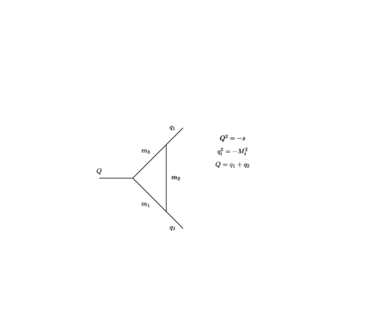
Figure 3: Triangle diagram: the general case with arbitrary internal and external masses.

From the Kershaw theorem [42] we see that the physical-region Landau curve has six branches in the $Q,q_{1},q_{2}$ space, i.e.

$$s>(m_{1}+m_{3})^{2}\,,\quad{\mathrm{M}}^{2}_{2}>(m_{2}+m_{3})^{2}\,,\quad{\mathrm{M}}^{2}_{1}<(m_{1}-m_{2})^{2}\,,$$ (35)

with $Q^{0}>0$ and $q^{0}_{2}>0$. The other branches are obtained by cyclic permutations and by the overall reflection of the external momenta. Our example will be as follows: there is an off-shell ${}{{}{{{{{\mathrm{{{}{}{{H}}\mspace{-0.6mu}}}}}}}}}$ with momentum $Q$ going to off-shell ${}{{}{{{{{\mathrm{{{}{}{{W}}\mspace{-0.6mu}}}}}}}}}$s; internal lines are ${}{{}{{{{{\mathrm{{{}{}{{t}}\mspace{-0.6mu}}}}}}}}},{}{{}{{{{{\mathrm{{{}{}{{b}}\mspace{-0.6mu}}}}}}}}}$ quarks, i.e.

$$m_{1}=m_{3}=m_{{}{{}{{{{{\mathrm{{{}{}{{t}}\mspace{-0.6mu}}}}}}}}}}\,,\qquad m_{2}=m_{{}{{}{{{{{\mathrm{{{}{}{{b}}\mspace{-0.6mu}}}}}}}}}}\,\,.$$ (36)

Furthermore, ${\mathrm{M}}_{2}>m_{{}{{}{{{{{\mathrm{{{}{}{{t}}\mspace{-0.6mu}}}}}}}}}}+m_{{}{{}{{{{{\mathrm{{{}{}{{b}}\mspace{-0.6mu}}}}}}}}}}$ and ${\mathrm{M}}_{1}<m_{{}{{}{{{{{\mathrm{{{}{}{{t}}\mspace{-0.6mu}}}}}}}}}}-m_{{}{{}{{{{{\mathrm{{{}{}{{b}}\mspace{-0.6mu}}}}}}}}}}$. In this configuration, when the ${}{{}{{{{{\mathrm{{{}{}{{t}}\mspace{-0.6mu}}}}}}}}}\,$-width is neglected, we obtain $X_{1.2}$, Gram and Cayley determinants,

$${\mathrm{G}}_{3} = -\frac{1}{4}\,{\mathrm{M}}^{2}_{2}+\frac{1}{2}\,(s+{\mathrm{M}}^{2}_{1})-\frac{1}{4}\,(s-{\mathrm{M}}^{2}_{1})^{2}\,,$$

$${\mathrm{C}}_{3} = -\frac{1}{4}\,m^{2}_{{}{{}{{{{{\mathrm{{{}{}{{t}}\mspace{-0.6mu}}}}}}}}}}\,{\mathrm{M}}^{4}_{2}+\frac{1}{4}\,\bigl{[}s\,(m^{2}_{{}{{}{{{{{\mathrm{{{}{}{{t}}\mspace{-0.6mu}}}}}}}}}}+m^{2}_{{}{{}{{{{{\mathrm{{{}{}{{b}}\mspace{-0.6mu}}}}}}}}}}-{\mathrm{M}}^{2}_{1})+2\,m^{2}_{{}{{}{{{{{\mathrm{{{}{}{{t}}\mspace{-0.6mu}}}}}}}}}}\,{\mathrm{M}}^{2}_{1}\bigr{]}$$

$$- \frac{1}{4}\,s\,(m^{2}_{{}{{}{{{{{\mathrm{{{}{}{{t}}\mspace{-0.6mu}}}}}}}}}}-m^{2}_{{}{{}{{{{{\mathrm{{{}{}{{b}}\mspace{-0.6mu}}}}}}}}}})^{2}+\frac{1}{4}\,s\,{\mathrm{M}}^{2}_{1}\,(m^{2}_{{}{{}{{{{{\mathrm{{{}{}{{t}}\mspace{-0.6mu}}}}}}}}}}+m^{2}_{{}{{}{{{{{\mathrm{{{}{}{{b}}\mspace{-0.6mu}}}}}}}}}})-\frac{1}{4}\,(m^{2}_{{}{{}{{{{{\mathrm{{{}{}{{t}}\mspace{-0.6mu}}}}}}}}}}\,{\mathrm{M}}^{4}_{1}+m^{2}_{{}{{}{{{{{\mathrm{{{}{}{{b}}\mspace{-0.6mu}}}}}}}}}}\,s^{2})\,,$$

$${\mathrm{G}}_{3}\,X_{1} = \frac{1}{4}\,(s+{\mathrm{M}}^{2}_{1}+m^{2}_{{}{{}{{{{{\mathrm{{{}{}{{t}}\mspace{-0.6mu}}}}}}}}}}-m^{2}_{{}{{}{{{{{\mathrm{{{}{}{{b}}\mspace{-0.6mu}}}}}}}}}})\,{\mathrm{M}}^{2}_{2}-\frac{1}{4}\,(s-m^{2}_{{}{{}{{{{{\mathrm{{{}{}{{t}}\mspace{-0.6mu}}}}}}}}}}+m^{2}_{{}{{}{{{{{\mathrm{{{}{}{{b}}\mspace{-0.6mu}}}}}}}}}})\,s-\frac{1}{4}\,({\mathrm{M}}^{2}_{1}+m^{2}_{{}{{}{{{{{\mathrm{{{}{}{{t}}\mspace{-0.6mu}}}}}}}}}}-m^{2}_{{}{{}{{{{{\mathrm{{{}{}{{b}}\mspace{-0.6mu}}}}}}}}}})\,{\mathrm{M}}^{2}_{1}+\frac{1}{2}\,s\,{\mathrm{M}}^{2}_{1}\,,$$

$${\mathrm{G}}_{3}\,X_{2} = \frac{1}{4}\,({\mathrm{M}}^{2}_{1}+m^{2}_{{}{{}{{{{{\mathrm{{{}{}{{t}}\mspace{-0.6mu}}}}}}}}}}-m^{2}_{{}{{}{{{{{\mathrm{{{}{}{{b}}\mspace{-0.6mu}}}}}}}}}})\,{\mathrm{M}}^{2}_{2}+\frac{1}{4}\,({\mathrm{M}}^{2}_{1}-m^{2}_{{}{{}{{{{{\mathrm{{{}{}{{t}}\mspace{-0.6mu}}}}}}}}}}+m^{2}_{{}{{}{{{{{\mathrm{{{}{}{{b}}\mspace{-0.6mu}}}}}}}}}})\,s-\frac{1}{4}\,({\mathrm{M}}^{2}_{1}+m^{2}_{{}{{}{{{{{\mathrm{{{}{}{{t}}\mspace{-0.6mu}}}}}}}}}}-m^{2}_{{}{{}{{{{{\mathrm{{{}{}{{b}}\mspace{-0.6mu}}}}}}}}}})\,{\mathrm{M}}^{2}_{1}\,,$$ (37)

The condition $\Delta_{3}=0$, at $\Gamma_{{}{{}{{{{{\mathrm{{{}{}{{t}}\mspace{-0.6mu}}}}}}}}}}=0$, can be seen as a quadratic equation in ${\mathrm{M}}^{2}_{2}$ for fixed $s$ and ${\mathrm{M}}_{1}$. Therefore, we require

$$[{\mathrm{T}}_{1}] \qquad\Delta_{3}\,=\,0\,,$$ (38)

$$[{\mathrm{T}}_{2}] \qquad 0\,<\,X_{2}\,<\,X_{1}\,<\,1\,,$$

$$[{\mathrm{T}}_{3}] \qquad s\,>\,({\mathrm{M}}_{1}+{\mathrm{M}}_{2})^{2}\,\,.$$

The space-time picture is the following: the state of momentum $Q$ decays into a ${}{}{{}{{}{{{{{\mathrm{{{}{}{{\overline{{}{{}{{{{{\mathrm{{{}{}{{t}}\mspace{-0.6mu}}}}}}}}}}}_{{\mspace{1.0mu}}}^{\mspace{1.0mu}{{\raisebox{-1.65764pt}{{${{{\scriptstyle{{{{{\mathrm{{}}}}}}}}}}$}}}}}}\mspace{-0.6mu}}}}}}}}}}{}{{}{{{{{\mathrm{{{}{}{{t}}\mspace{-0.6mu}}}}}}}}}$ pair, one of the top quarks decays into ${}{{}{{{{{\mathrm{{{}{}{{W}}\mspace{-0.6mu}}}}}}}}}{}{{}{{{{{\mathrm{{{}{}{{b}}\mspace{-0.6mu}}}}}}}}}$, the ${}{{}{{{{{\mathrm{{{}{}{{b}}\mspace{-0.6mu}}}}}}}}}$ quark rescatters against the second ${}{{}{{{{{\mathrm{{{}{}{{t}}\mspace{-0.6mu}}}}}}}}}$ quark to produce a state with invariant mass ${\mathrm{M}}_{2}$. The solution of $\Delta_{3}=0$ can give complex ${\mathrm{M}}^{2}_{2}$, ${\mathrm{M}}^{2}_{2}$, real but negative, a real solution which does not satisfy condition $[{\mathrm{T}}_{2}]$ in Eq.(38), a real solution satisfying $[{\mathrm{T}}_{2}]$ (the $X$ test) but not $[{\mathrm{T}}_{3}]$ (singularity inside the physical region) and, finally, a physical singularity satisfying both $[{\mathrm{T}}_{2}]$ and $[{\mathrm{T}}_{3}]$. The distribution of physical-region singularities ($\Gamma_{{}{{}{{{{{\mathrm{{{}{}{{t}}\mspace{-0.6mu}}}}}}}}}}=0$) is shown in Figure 4 in the $\sqrt{s}{-}{\mathrm{M}}_{1}$ plane with $350~{}\text{GeV}<\sqrt{s}<750~{}\text{GeV}$ and ${\mathrm{M}}_{1,2}>10~{}\text{GeV}$.

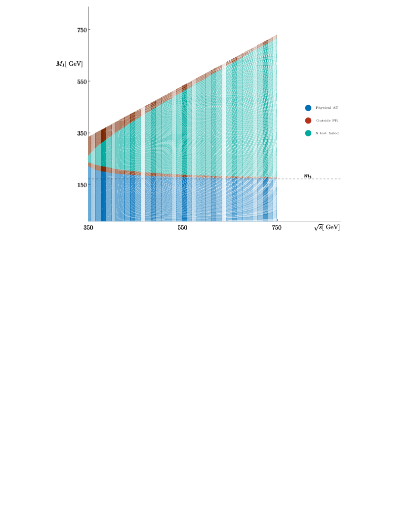
Figure 4: Physical and non physical AT for the triangle diagram of Figure 3 with internal masses given in Eq.(36). Here $350~{}\text{GeV}<\sqrt{s}<750~{}\text{GeV}$ and ${\mathrm{M}}_{1,2}>10~{}\text{GeV}$. For given values of $\sqrt{s}$ and ${\mathrm{M}}_{1}$ the value of ${\mathrm{M}}_{2}$ corresponding to the AT is computed.

To study the corresponding Peierls zeros we introduce $s_{\pm}={\mathrm{M}}^{2}_{1}\pm{\mathrm{M}}^{2}_{2}$ and derive that

$$s_{+}=\frac{s^{2}_{-}}{s}+2\,(m^{2}_{{}{{}{{{{{\mathrm{{{}{}{{t}}\mspace{-0.6mu}}}}}}}}}}-m^{2}_{{}{{}{{{{{\mathrm{{{}{}{{b}}\mspace{-0.6mu}}}}}}}}}})\,,\quad s^{2}_{-}=\frac{s}{2}\,\Bigl{\{}s-4\,m^{2}_{{}{{}{{{{{\mathrm{{{}{}{{t}}\mspace{-0.6mu}}}}}}}}}}+8\,m^{2}_{{}{{}{{{{{\mathrm{{{}{}{{b}}\mspace{-0.6mu}}}}}}}}}}\pm\Bigl{[}(s-4\,m^{2}_{{}{{}{{{{{\mathrm{{{}{}{{t}}\mspace{-0.6mu}}}}}}}}}})^{2}+16\,\Gamma^{2}_{{}{{}{{{{{\mathrm{{{}{}{{t}}\mspace{-0.6mu}}}}}}}}}}\,m^{2}_{{}{{}{{{{{\mathrm{{{}{}{{t}}\mspace{-0.6mu}}}}}}}}}}\Bigr{]}^{1/2}\Bigr{\}}$$ (39)

satisfy $\mathop{\mathrm{Re}}\nolimits\,\Delta_{3}=\mathop{\mathrm{Im}}\nolimits\,\Delta_{3}=0$. Neglecting the ${}{{}{{{{{\mathrm{{{}{}{{b}}\mspace{-0.6mu}}}}}}}}}$ width and using the leading-order (LO) value for $\Gamma_{{}{{}{{{{{\mathrm{{{}{}{{t}}\mspace{-0.6mu}}}}}}}}}}$ we find no Peierls zeros inside the physical region defined by $s>({\mathrm{M}}_{1}+{\mathrm{M}}_{2})^{2}$. For instance, for $\sqrt{s}=350~{}\text{GeV}$, the zero corresponds to invariant masses of $486.3~{}\text{GeV}$ and $254.0~{}\text{GeV}$ or to a negative value for $s^{2}_{-}$.

We give an example in Figure 5 where we plot ${\mathrm{L}}(s\,C_{0})$ as a function of ${\mathrm{M}}_{2}$ for $\sqrt{s}=350~{}\text{GeV}$, ${\mathrm{M}}_{1}=120~{}\text{GeV}$ and where the log-modulus function [74] is

$${\mathrm{L}}(x)=\mbox{sign}(x)\,\frac{\ln(1+\mid\,x\,\mid)}{\ln\,10}\,\,.$$ (40)

The effect of the normal threshold, ${\mathrm{M}}_{2}=m_{{}{{}{{{{{\mathrm{{{}{}{{t}}\mspace{-0.6mu}}}}}}}}}}+m_{{}{{}{{{{{\mathrm{{{}{}{{b}}\mspace{-0.6mu}}}}}}}}}}$, and of the anomalous threshold , ${\mathrm{M}}_{2}=201.89~{}\text{GeV}$ are clearly visible in the real part (solid line) and in the imaginary one (dashed line). Red curves correspond to the choice of $\Gamma_{{}{{}{{{{{\mathrm{{{}{}{{t}}\mspace{-0.6mu}}}}}}}}}}/100$.

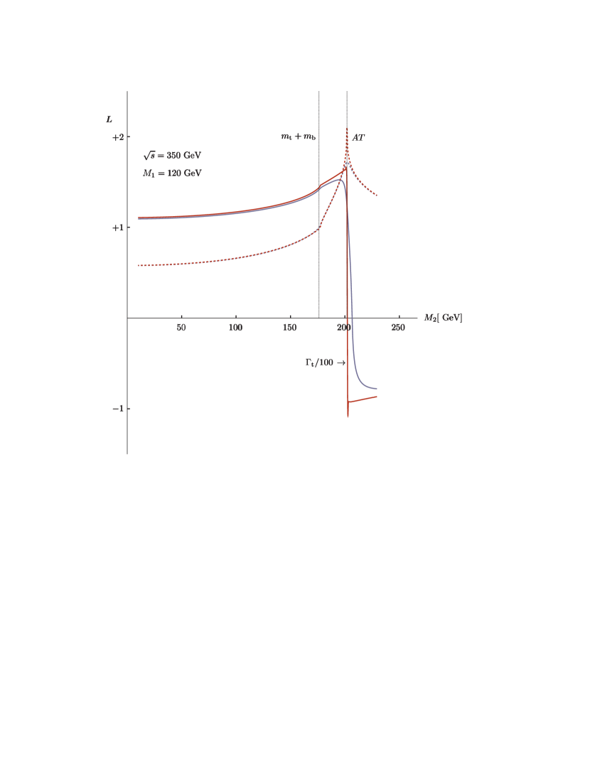
Figure 5: The log-modulus transformation of $s\,C_{0}$ as a function of ${\mathrm{M}}_{2}$ for $\sqrt{s}=350~{}\text{GeV}$, ${\mathrm{M}}_{1}=120~{}\text{GeV}$. The red curves correspond to $\Gamma_{{}{{}{{{{{\mathrm{{{}{}{{t}}\mspace{-0.6mu}}}}}}}}}}/100$.

The ${\mathrm{M}}_{2}$ distribution is also shown in Figure 6 for $\sqrt{s}=350~{}\text{GeV}$ and different values of ${\mathrm{M}}_{1}$. It can be seen that higher values for ${\mathrm{M}}_{1}$ produce lower values for the AT.

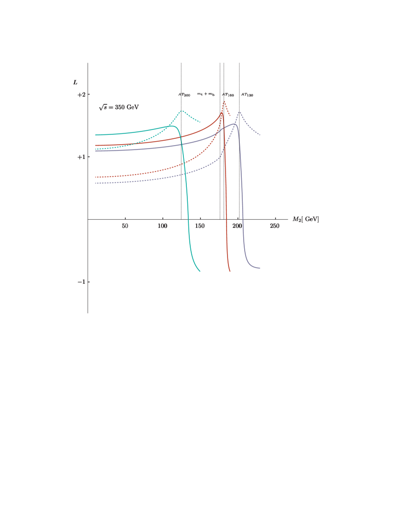
Figure 6: The log-modulus transformation of $s\,C_{0}$ as a function of ${\mathrm{M}}_{2}$ for $\sqrt{s}=350~{}\text{GeV}$, and ${\mathrm{M}}_{1}=120~{}\text{GeV}$ (blue), ${\mathrm{M}}_{1}=160~{}\text{GeV}$ (red) and ${\mathrm{M}}_{1}=200~{}\text{GeV}$ (emerald). Solid curves give the real part while dashed curves give the imaginary part.

In order to understand the impact of the AT on some realistic distribution we introduce the ${}{{}{{{{{\mathrm{{{}{}{{W}}\mspace{-0.6mu}}}}}}}}}$ complex pole, $s_{{\scriptscriptstyle{{}{{}{{{{{\mathrm{{{}{}{{W}}\mspace{-0.6mu}}}}}}}}}}}}=\mu^{2}_{{\scriptscriptstyle{{}{{}{{{{{\mathrm{{{}{}{{W}}\mspace{-0.6mu}}}}}}}}}}}}-i\,\mu_{{\scriptscriptstyle{{}{{}{{{{{\mathrm{{{}{}{{W}}\mspace{-0.6mu}}}}}}}}}}}}\,\gamma_{{\scriptscriptstyle{{}{{}{{{{{\mathrm{{{}{}{{W}}\mspace{-0.6mu}}}}}}}}}}}}$ and define

$${\mathrm{C}}_{\Delta}({\mathrm{M}}_{1})=s^{4}\,\Delta_{{\scriptscriptstyle{{}{{}{{{{{\mathrm{{{}{}{{W}}\mspace{-0.6mu}}}}}}}}}}}}({\mathrm{M}}_{1})\,\int_{{\mathrm{M}}^{2}_{{\mathrm{c}}}}^{(\sqrt{s}-{\mathrm{M}}_{1})^{2}}\,d{\mathrm{M}}^{2}_{2}\,\Delta_{{\scriptscriptstyle{{}{{}{{{{{\mathrm{{{}{}{{W}}\mspace{-0.6mu}}}}}}}}}}}}({\mathrm{M}}_{2})\,\mathop{\mathrm{Re}}\nolimits\,{\mathrm{C}}_{0}(s\,,\,{\mathrm{M}}^{2}_{1}\,,\,{\mathrm{M}}^{2}_{2}\,;\,m_{{}{{}{{{{{\mathrm{{{}{}{{t}}\mspace{-0.6mu}}}}}}}}}}\,,\,m_{{}{{}{{{{{\mathrm{{{}{}{{b}}\mspace{-0.6mu}}}}}}}}}}\,,\,m_{{}{{}{{{{{\mathrm{{{}{}{{t}}\mspace{-0.6mu}}}}}}}}}})\,,$$ (41)

where the propagator factor is

$$\Delta_{{\scriptscriptstyle{{}{{}{{{{{\mathrm{{{}{}{{W}}\mspace{-0.6mu}}}}}}}}}}}}({\mathrm{M}})=\frac{1}{\mid{\mathrm{M}}^{2}-s_{{\scriptscriptstyle{{}{{}{{{{{\mathrm{{{}{}{{W}}\mspace{-0.6mu}}}}}}}}}}}}\mid^{2}}\,,$$ (42)

and where ${\mathrm{M}}_{{\mathrm{c}}}$ is a lower cut on ${\mathrm{M}}_{2}$. We show ${\mathrm{L}}({\mathrm{C}}_{\Delta})$ (Eq.(40)) in Figure 7 for $3$ values of $\sqrt{s}$.

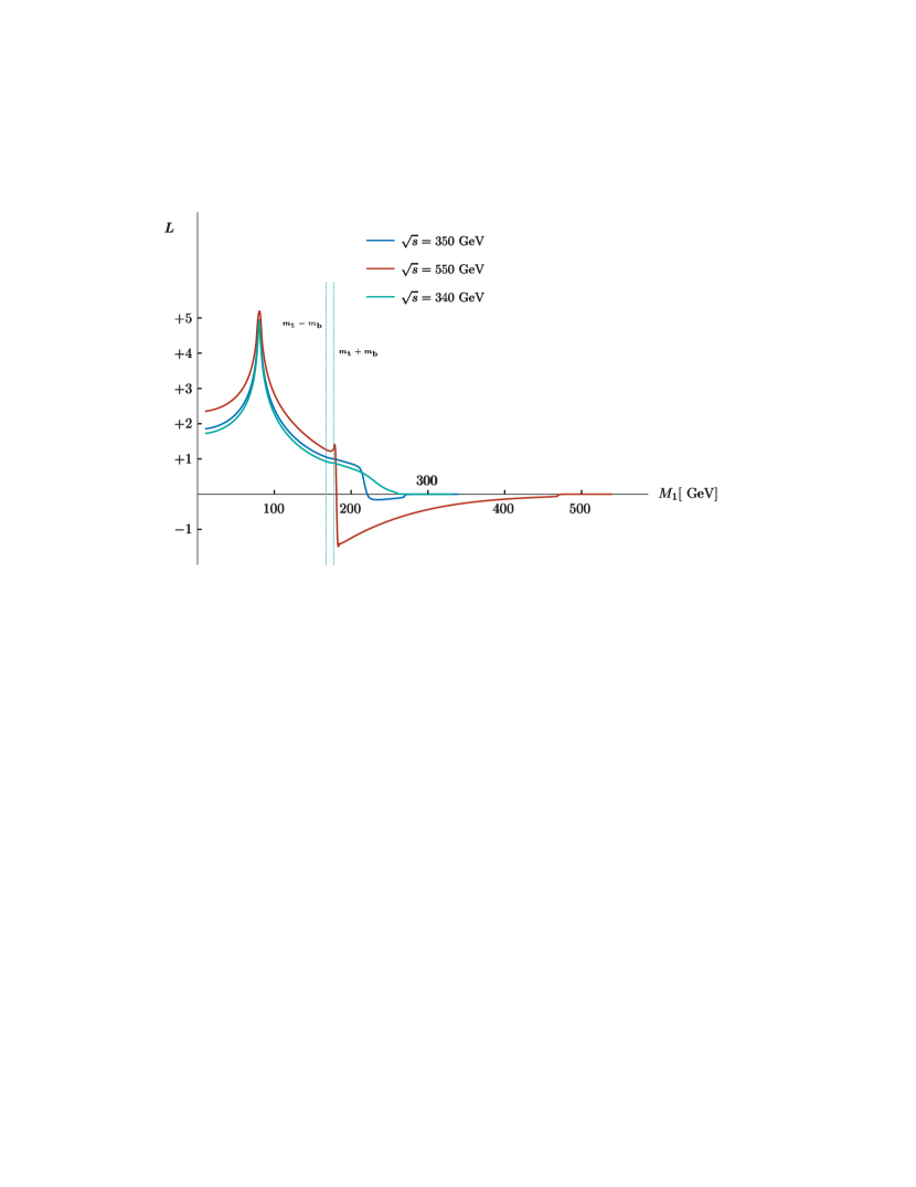
Figure 7: ${\mathrm{L}}({\mathrm{C}}_{\Delta})$ as a function of ${\mathrm{M}}_{1}$ for different values of $\sqrt{s}$. ${\mathrm{C}}_{\Delta}$ is defined in Eq.(41) and ${\mathrm{L}}(x)$ in Eq.(40).

In order to understand the behavior of different curves in Figure 7 we recall that the occurrence of the AT requires $\sqrt{s}>2\,m_{{}{{}{{{{{\mathrm{{{}{}{{t}}\mspace{-0.6mu}}}}}}}}}}$, therefore there is no AT for $\sqrt{s}=340~{}\text{GeV}$. Furthermore we must have ${\mathrm{M}}_{1}>m_{{}{{}{{{{{\mathrm{{{}{}{{t}}\mspace{-0.6mu}}}}}}}}}}+m_{{}{{}{{{{{\mathrm{{{}{}{{b}}\mspace{-0.6mu}}}}}}}}}}$ and ${\mathrm{M}}_{2}<m_{{}{{}{{{{{\mathrm{{{}{}{{t}}\mspace{-0.6mu}}}}}}}}}}-m_{{}{{}{{{{{\mathrm{{{}{}{{b}}\mspace{-0.6mu}}}}}}}}}}$ or ${\mathrm{M}}_{1}<m_{{}{{}{{{{{\mathrm{{{}{}{{t}}\mspace{-0.6mu}}}}}}}}}}-m_{{}{{}{{{{{\mathrm{{{}{}{{b}}\mspace{-0.6mu}}}}}}}}}}$ and ${\mathrm{M}}_{2}>m_{{}{{}{{{{{\mathrm{{{}{}{{t}}\mspace{-0.6mu}}}}}}}}}}+m_{{}{{}{{{{{\mathrm{{{}{}{{b}}\mspace{-0.6mu}}}}}}}}}}$, with ${\mathrm{M}}_{1}+{\mathrm{M}}_{2}<\sqrt{s}$. The equation $\Delta_{3}=0$ is quadratic in ${\mathrm{M}}_{2}$ and can be solved for fixed $\sqrt{s},{\mathrm{M}}_{1}$ and the solutions must satisfy conditions ${\mathrm{T}}_{2,3}$ in Eq.(38). We find that at most one of the two solutions does it, as expected. In particular, for $\sqrt{s}=350~{}\text{GeV}$ we always find one real value for ${\mathrm{M}}_{2}$ that corresponds to the AT if ${\mathrm{M}}_{1}<168~{}\text{GeV}$; ${\mathrm{M}}_{2}$ is complex for $168~{}\text{GeV}<{\mathrm{M}}_{1}<177~{}\text{GeV}$ with tiny imaginary part; ${\mathrm{M}}_{2}$ is again real for $177~{}\text{GeV}<{\mathrm{M}}_{1}<226~{}\text{GeV}$ and becomes imaginary for ${\mathrm{M}}_{1}>226~{}\text{GeV}$.

Finally, we consider the process ${}{{}{{{{{\mathrm{{{}{}{{g}}\mspace{-0.6mu}}}}}}}}}{}{{}{{{{{\mathrm{{{}{}{{g}}\mspace{-0.6mu}}}}}}}}}\to{}{{}{{{{{\mathrm{{{}{}{{{}{{}{{{{{\mathrm{{{}{}{{e}}\mspace{-0.6mu}}}}}}}}}}^{-}}\mspace{-0.6mu}}}}}}}}}{}{{}{{{{{\mathrm{{{}{}{{{}{{}{{{{{\mathrm{{{}{}{}\mspace{-0.6mu}}}}}}}}}}^{+}}\mspace{-0.6mu}}}}}}}}}{}{}{{}{{}{{{{{\mathrm{{{}{}{{\overline{{}{{}{{{{{\mathrm{{{}{}{}\mspace{-0.6mu}}}}}}}}}}}_{{\mspace{1.0mu}\!{}{{}{{{{{\mathrm{{{}{}{{e}}\mspace{-0.6mu}}}}}}}}}}}^{\mspace{1.0mu}{{\raisebox{-1.65764pt}{{${{{\scriptstyle{{{{{\mathrm{{}}}}}}}}}}$}}}}}}\mspace{-0.6mu}}}}}}}}}}{}{{}{{{{{\mathrm{{{}{}{{{}{{}{{{{{\mathrm{{{}{}{}\mspace{-0.6mu}}}}}}}}}}_{{\!{}{{}{{{{{\mathrm{{{}{}{}\mspace{-0.6mu}}}}}}}}}}}}\mspace{-0.6mu}}}}}}}}}$, in particular the ${}{{}{{{{{\mathrm{{{}{}{{g}}\mspace{-0.6mu}}}}}}}}}{}{{}{{{{{\mathrm{{{}{}{{g}}\mspace{-0.6mu}}}}}}}}}\to{}{{}{{{{{\mathrm{{{}{}{{H}}\mspace{-0.6mu}}}}}}}}}\to{}{{}{{{{{\mathrm{{{}{}{{{}{{}{{{{{\mathrm{{{}{}{{e}}\mspace{-0.6mu}}}}}}}}}}^{-}}\mspace{-0.6mu}}}}}}}}}{}{{}{{{{{\mathrm{{{}{}{{{}{{}{{{{{\mathrm{{{}{}{}\mspace{-0.6mu}}}}}}}}}}^{+}}\mspace{-0.6mu}}}}}}}}}{}{}{{}{{}{{{{{\mathrm{{{}{}{{\overline{{}{{}{{{{{\mathrm{{{}{}{}\mspace{-0.6mu}}}}}}}}}}}_{{\mspace{1.0mu}\!{}{{}{{{{{\mathrm{{{}{}{{e}}\mspace{-0.6mu}}}}}}}}}}}^{\mspace{1.0mu}{{\raisebox{-1.65764pt}{{${{{\scriptstyle{{{{{\mathrm{{}}}}}}}}}}$}}}}}}\mspace{-0.6mu}}}}}}}}}}{}{{}{{{{{\mathrm{{{}{}{{{}{{}{{{{{\mathrm{{{}{}{}\mspace{-0.6mu}}}}}}}}}}_{{\!{}{{}{{{{{\mathrm{{{}{}{}\mspace{-0.6mu}}}}}}}}}}}}\mspace{-0.6mu}}}}}}}}}$ component. The question of gauge invariance has been discussed at length in Ref. [90]: given the process ${}{{}{{{{{\mathrm{{{}{}{{g}}\mspace{-0.6mu}}}}}}}}}{}{{}{{{{{\mathrm{{{}{}{{g}}\mspace{-0.6mu}}}}}}}}}\to{}{{}{{{{{\mathrm{{{}{}{{F}}\mspace{-0.6mu}}}}}}}}}$, where ${}{{}{{{{{\mathrm{{{}{}{{F}}\mspace{-0.6mu}}}}}}}}}$ is an arbitrary final state we want to separate the ${}{{}{{{{{\mathrm{{{}{}{{H}}\mspace{-0.6mu}}}}}}}}}$ component as

$$\sigma_{{}{{}{{{{{\mathrm{{{}{}{{g}}\mspace{-0.6mu}}}}}}}}}{}{{}{{{{{\mathrm{{{}{}{{g}}\mspace{-0.6mu}}}}}}}}}\to{}{{}{{{{{\mathrm{{{}{}{{H}}\mspace{-0.6mu}}}}}}}}}\to{}{{}{{{{{\mathrm{{{}{}{{F}}\mspace{-0.6mu}}}}}}}}}}(s)=\frac{1}{\pi}\,\sigma_{{}{{}{{{{{\mathrm{{{}{}{{g}}\mspace{-0.6mu}}}}}}}}}{}{{}{{{{{\mathrm{{{}{}{{g}}\mspace{-0.6mu}}}}}}}}}\to{}{{}{{{{{\mathrm{{{}{}{{H}}\mspace{-0.6mu}}}}}}}}}}\,s^{2}\,\Delta_{{\scriptscriptstyle{{}{{}{{{{{\mathrm{{{}{}{{H}}\mspace{-0.6mu}}}}}}}}}}}}(s)\,\frac{\Gamma_{{}{{}{{{{{\mathrm{{{}{}{{H}}\mspace{-0.6mu}}}}}}}}}\to{}{{}{{{{{\mathrm{{{}{}{{F}}\mspace{-0.6mu}}}}}}}}}}}{\sqrt{s}}\,\,.$$ (43)

where $s_{{\scriptscriptstyle{{}{{}{{{{{\mathrm{{{}{}{{H}}\mspace{-0.6mu}}}}}}}}}}}}$ is the Higgs complex pole. To summarize: we would like to use the Higgs propagator with its complex pole with production and decay computed at arbitrary Higgs virtuality and not at the complex pole. As far as LO production is concerned, e.g. the ${}{{}{{{{{\mathrm{{{}{}{{g}}\mspace{-0.6mu}}}}}}}}}{}{{}{{{{{\mathrm{{{}{}{{g}}\mspace{-0.6mu}}}}}}}}}{}{{}{{{{{\mathrm{{{}{}{{H}}\mspace{-0.6mu}}}}}}}}}$ one-loop fermion triangle, there is never an issue of gauge-parameter dependence in going off-shell; in this respect higher order QCD corrections are not a problem.

Consider now the decay, i.e. $\Gamma({}{{}{{{{{\mathrm{{{}{}{{H}}\mspace{-0.6mu}}}}}}}}}\to{}{{}{{{{{\mathrm{{{}{}{{F}}\mspace{-0.6mu}}}}}}}}})$ in Eq.(43): the amplitude ${\mathrm{A}}({}{{}{{{{{\mathrm{{{}{}{{H}}\mspace{-0.6mu}}}}}}}}}\to{}{{}{{{{{\mathrm{{{}{}{{F}}\mspace{-0.6mu}}}}}}}}})$, for each final state and as long as we include the complete set of diagrams at one-loop order, is gauge-parameter independent if the Higgs boson is on its mass-shell. However, as soon as we put an external leg off-shell, the amplitude must be coupled to the corresponding physical source and only the complete process ${}{{}{{{{{\mathrm{{{}{}{{I}}\mspace{-0.6mu}}}}}}}}}\to{}{{}{{{{{\mathrm{{{}{}{{F}}\mspace{-0.6mu}}}}}}}}}$ is gauge-parameter independent. The latter does not exclude the existence of subsets of diagrams that satisfy the requirement but this can only be examined on a case-by-case basis. To rephrase it, if the Higgs boson is off shell, the matrix element still respects gauge invariance (in most cases) in LO and in next-to-leading (NLO) QCD but in NLO EW gauge invariance is lost. How to deal with this situation? Technically speaking, we have a matrix element

$$\Gamma\left({}{{}{{{{{\mathrm{{{}{}{{H}}\mspace{-0.6mu}}}}}}}}}\to{}{{}{{{{{\mathrm{{{}{}{{F}}\mspace{-0.6mu}}}}}}}}}\right)=f\left(s\,,\,\mu^{2}_{{}{{}{{{{{\mathrm{{{}{}{{H}}\mspace{-0.6mu}}}}}}}}}}\right),$$ (44)

where $s$ is the virtuality of the external Higgs boson, $\mu_{{}{{}{{{{{\mathrm{{{}{}{{H}}\mspace{-0.6mu}}}}}}}}}}$ is the mass of internal Higgs lines and Higgs wave-function renormalization has been included. The following happens: $f(s_{{\scriptscriptstyle{{}{{}{{{{{\mathrm{{{}{}{{H}}\mspace{-0.6mu}}}}}}}}}}}}\,,\,s_{{\scriptscriptstyle{{}{{}{{{{{\mathrm{{{}{}{{H}}\mspace{-0.6mu}}}}}}}}}}}})$ is gauge-parameter independent to all orders while $f(\mu^{2}_{{}{{}{{{{{\mathrm{{{}{}{{H}}\mspace{-0.6mu}}}}}}}}}}\,,\,\mu^{2}_{{}{{}{{{{{\mathrm{{{}{}{{H}}\mspace{-0.6mu}}}}}}}}}})$ is gauge-parameter independent at one-loop but not beyond, $f(s\,,\,\mu^{2}_{{}{{}{{{{{\mathrm{{{}{}{{H}}\mspace{-0.6mu}}}}}}}}}})$ is not. In order to account for the off-shellness of the Higgs boson we defined a viable scheme by choosing (at one loop level) $f(s\,,\,s)$, i.e. we intuitively replace the on-shell decay of the Higgs boson of mass $\mu_{{}{{}{{{{{\mathrm{{{}{}{{H}}\mspace{-0.6mu}}}}}}}}}}$ with the on-shell decay of an Higgs boson of mass $\sqrt{s}$ and not with the off-shell decay of an Higgs boson of mass $\mu_{{}{{}{{{{{\mathrm{{{}{}{{H}}\mspace{-0.6mu}}}}}}}}}}$. The same applies for the NLO EW correction to production.

In our case we are interested in the effect of the AT present in the triangle graph ${}{{}{{{{{\mathrm{{{}{}{{H}}\mspace{-0.6mu}}}}}}}}}{}{{}{{{{{\mathrm{{{}{}{{W}}\mspace{-0.6mu}}}}}}}}}{}{{}{{{{{\mathrm{{{}{}{{W}}\mspace{-0.6mu}}}}}}}}}$ with internal quark lines and, therefore, there is no problem in the off-shellness of the process (there are no internal Higgs lines); furthermore, no other diagram produces an AT (at the same location). As a consequence we can analyze ${}{{}{{{{{\mathrm{{{}{}{{H}}\mspace{-0.6mu}}}}}}}}}\to{}{{}{{{{{\mathrm{{{}{}{{{}{{}{{{{{\mathrm{{{}{}{{e}}\mspace{-0.6mu}}}}}}}}}}^{-}}\mspace{-0.6mu}}}}}}}}}{}{{}{{{{{\mathrm{{{}{}{{{}{{}{{{{{\mathrm{{{}{}{}\mspace{-0.6mu}}}}}}}}}}^{+}}\mspace{-0.6mu}}}}}}}}}{}{}{{}{{}{{{{{\mathrm{{{}{}{{\overline{{}{{}{{{{{\mathrm{{{}{}{}\mspace{-0.6mu}}}}}}}}}}}_{{\mspace{1.0mu}\!{}{{}{{{{{\mathrm{{{}{}{{e}}\mspace{-0.6mu}}}}}}}}}}}^{\mspace{1.0mu}{{\raisebox{-1.65764pt}{{${{{\scriptstyle{{{{{\mathrm{{}}}}}}}}}}$}}}}}}\mspace{-0.6mu}}}}}}}}}}{}{{}{{{{{\mathrm{{{}{}{{{}{{}{{{{{\mathrm{{{}{}{}\mspace{-0.6mu}}}}}}}}}}_{{\!{}{{}{{{{{\mathrm{{{}{}{}\mspace{-0.6mu}}}}}}}}}}}}\mspace{-0.6mu}}}}}}}}}$ with off-shell ${}{{}{{{{{\mathrm{{{}{}{{H}}\mspace{-0.6mu}}}}}}}}}$ and look for the impact of the AT on $\Gamma({}{{}{{{{{\mathrm{{{}{}{{H}}\mspace{-0.6mu}}}}}}}}}\to{}{{}{{{{{\mathrm{{{}{}{{{}{{}{{{{{\mathrm{{{}{}{{e}}\mspace{-0.6mu}}}}}}}}}}^{-}}\mspace{-0.6mu}}}}}}}}}{}{{}{{{{{\mathrm{{{}{}{{{}{{}{{{{{\mathrm{{{}{}{}\mspace{-0.6mu}}}}}}}}}}^{+}}\mspace{-0.6mu}}}}}}}}}{}{}{{}{{}{{{{{\mathrm{{{}{}{{\overline{{}{{}{{{{{\mathrm{{{}{}{}\mspace{-0.6mu}}}}}}}}}}}_{{\mspace{1.0mu}\!{}{{}{{{{{\mathrm{{{}{}{{e}}\mspace{-0.6mu}}}}}}}}}}}^{\mspace{1.0mu}{{\raisebox{-1.65764pt}{{${{{\scriptstyle{{{{{\mathrm{{}}}}}}}}}}$}}}}}}\mspace{-0.6mu}}}}}}}}}}{}{{}{{{{{\mathrm{{{}{}{{{}{{}{{{{{\mathrm{{{}{}{}\mspace{-0.6mu}}}}}}}}}}_{{\!{}{{}{{{{{\mathrm{{{}{}{}\mspace{-0.6mu}}}}}}}}}}}}\mspace{-0.6mu}}}}}}}}})$. The process is now

$${}{{}{{{{{\mathrm{{{}{}{{H}}\mspace{-0.6mu}}}}}}}}}(Q)\to{}{{}{{{{{\mathrm{{{}{}{{{}{{}{{{{{\mathrm{{{}{}{{W}}\mspace{-0.6mu}}}}}}}}}}^{+}}\mspace{-0.6mu}}}}}}}}}(q_{1}+q_{2})+{}{{}{{{{{\mathrm{{{}{}{{{}{{}{{{{{\mathrm{{{}{}{{W}}\mspace{-0.6mu}}}}}}}}}}^{-}}\mspace{-0.6mu}}}}}}}}}(q_{3}+q_{4})\to{}{{}{{{{{\mathrm{{{}{}{{{}{{}{{{{{\mathrm{{{}{}{}\mspace{-0.6mu}}}}}}}}}}_{{\!{}{{}{{{{{\mathrm{{{}{}{}\mspace{-0.6mu}}}}}}}}}}}}\mspace{-0.6mu}}}}}}}}}(q_{1})+{}{{}{{{{{\mathrm{{{}{}{{{}{{}{{{{{\mathrm{{{}{}{}\mspace{-0.6mu}}}}}}}}}}^{+}}\mspace{-0.6mu}}}}}}}}}(q_{2})+{}{{}{{{{{\mathrm{{{}{}{{{}{{}{{{{{\mathrm{{{}{}{{e}}\mspace{-0.6mu}}}}}}}}}}^{-}}\mspace{-0.6mu}}}}}}}}}(q_{3})+{}{}{{}{{}{{{{{\mathrm{{{}{}{{\overline{{}{{}{{{{{\mathrm{{{}{}{}\mspace{-0.6mu}}}}}}}}}}}_{{\mspace{1.0mu}\!{}{{}{{{{{\mathrm{{{}{}{{e}}\mspace{-0.6mu}}}}}}}}}}}^{\mspace{1.0mu}{{\raisebox{-1.65764pt}{{${{{\scriptstyle{{{{{\mathrm{{}}}}}}}}}}$}}}}}}\mspace{-0.6mu}}}}}}}}}}(q_{4})\,,$$ (45)

with $Q^{2}=-s$ and light fermion masses are neglected. The full process is given in terms of $s$ and $5$ additional Mandelstam invariants [91],

$$s_{1} = -(q_{2}+q_{3}+q_{4})^{2}\,,\qquad s_{2}=-(q_{3}+q_{4})^{2}\,,$$

$$u_{1} = -(q_{1}+q_{3}+q_{4})^{2}\,,\qquad u_{2}=-(q_{1}+q_{2}+q_{4})^{2}\,,$$

$$t_{2} = -(q_{1}+q_{4})^{2}\,\,.$$ (46)

Next we define $s_{2}={\mathrm{M}}^{2}$ and study the $d\Gamma/d{\mathrm{M}}$ distribution,

$$\frac{d\Gamma}{d{\mathrm{M}}}=\frac{d\Gamma}{d{\mathrm{M}}}\Bigr{|}_{\mathrm{\scriptscriptstyle{LO}}}+\frac{d\Gamma}{d{\mathrm{M}}}\Bigr{|}_{\mathrm{\scriptscriptstyle{NLO}}\,,\,\mathrm{\scriptscriptstyle{AT}}}+\frac{d\Gamma}{d{\mathrm{M}}}\Bigr{|}_{\mathrm{\scriptscriptstyle{NLO}}\,,\,{\mbox{\scriptsize rest}}}\,\,.$$ (47)

Since our interest is, in the first place, on the AT effect we limit the calculation to $\delta_{\mathrm{\scriptscriptstyle{AT}}}$, the percentage correction introduced by the AT.

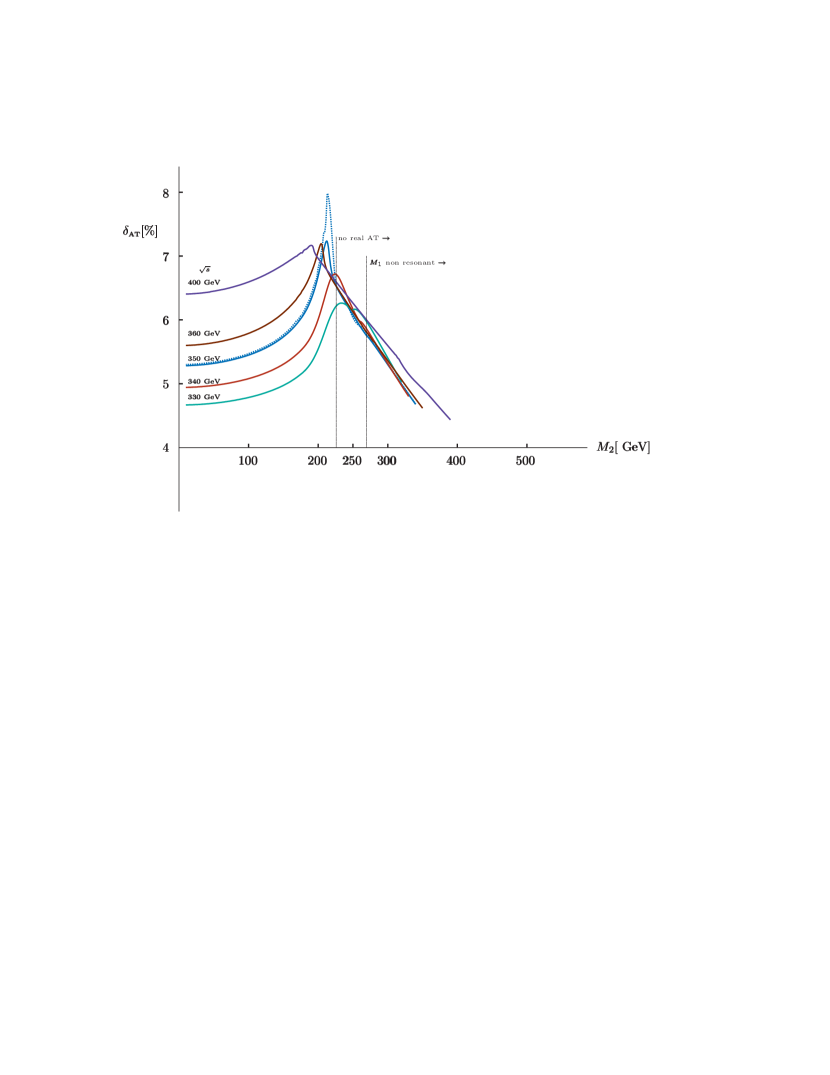
Figure 8: Percentage radiative corrections around the AT (Eq.(47)) for the process of Eq.(45).

Results are shown in Figure 8 for different values of $\sqrt{s}$. To understand the behavior of radiative corrections two effects should be taken into account: ${\mathrm{M}}_{1}$ is non resonant if ${\mathrm{M}}_{2}>\sqrt{s}-M_{{}{{}{{{{{\mathrm{{{}{}{{W}}\mspace{-0.6mu}}}}}}}}}}$ and above a certain value for ${\mathrm{M}}_{2}$ there is no AT corresponding to a real value of ${\mathrm{M}}_{1}$. For instance, for $\sqrt{s}=350~{}\text{GeV}$ this happens above ${\mathrm{M}}_{2}\approx 226~{}\text{GeV}$. The (blue) dashed line corresponds to $\sqrt{s}=350~{}\text{GeV}$ and $\Gamma_{{}{{}{{{{{\mathrm{{{}{}{{t}}\mspace{-0.6mu}}}}}}}}}}\to\Gamma_{{}{{}{{{{{\mathrm{{{}{}{{t}}\mspace{-0.6mu}}}}}}}}}}/100$, showing the effect of the AT.

4.1 AT induced by QCD/QED radiation

It is easy to see that there is no AT for ${}{{}{{{{{\mathrm{{{}{}{{X}}\mspace{-0.6mu}}}}}}}}}\to{}{}{{}{{}{{{{{\mathrm{{{}{}{{\overline{{}{{}{{{{{\mathrm{{{}{}{{f}}\mspace{-0.6mu}}}}}}}}}}}_{{\mspace{1.0mu}}}^{\mspace{1.0mu}{{\raisebox{-1.65764pt}{{${{{\scriptstyle{{{{{\mathrm{{}}}}}}}}}}$}}}}}}\mspace{-0.6mu}}}}}}}}}}{}{{}{{{{{\mathrm{{{}{}{{f}}\mspace{-0.6mu}}}}}}}}}$, where ${}{{}{{{{{\mathrm{{{}{}{{X}}\mspace{-0.6mu}}}}}}}}}$ can be an on-shell BSM Higgs boson, the off-shell SM Higgs boson or an off-shell ${}{{}{{{{{\mathrm{{{}{}{{Z}}\mspace{-0.6mu}}}}}}}}}$ boson. However, considering the processes

$${}{{}{{{{{\mathrm{{{}{}{{X}}\mspace{-0.6mu}}}}}}}}}\to{}{}{{}{{}{{{{{\mathrm{{{}{}{{\overline{{}{{}{{{{{\mathrm{{{}{}{{b}}\mspace{-0.6mu}}}}}}}}}}}_{{\mspace{1.0mu}}}^{\mspace{1.0mu}{{\raisebox{-1.65764pt}{{${{{\scriptstyle{{{{{\mathrm{{}}}}}}}}}}$}}}}}}\mspace{-0.6mu}}}}}}}}}}{}{{}{{{{{\mathrm{{{}{}{{b}}\mspace{-0.6mu}}}}}}}}}{}{{}{{{{{\mathrm{{{}{}{{g}}\mspace{-0.6mu}}}}}}}}}\,,\qquad{}{{}{{{{{\mathrm{{{}{}{{X}}\mspace{-0.6mu}}}}}}}}}\to{}{}{{}{{}{{{{{\mathrm{{{}{}{{\overline{{}{{}{{{{{\mathrm{{{}{}{{f}}\mspace{-0.6mu}}}}}}}}}}}_{{\mspace{1.0mu}}}^{\mspace{1.0mu}{{\raisebox{-1.65764pt}{{${{{\scriptstyle{{{{{\mathrm{{}}}}}}}}}}$}}}}}}\mspace{-0.6mu}}}}}}}}}}{}{{}{{{{{\mathrm{{{}{}{{f}}\mspace{-0.6mu}}}}}}}}}{}{{}{{{{{\mathrm{{{}{}{}\mspace{-0.6mu}}}}}}}}}\,,$$ (48)

we find a class of one-loop diagrams (a representative is a) in Figure 9) which admit a physical-region AT. The processes shown in Eq.(48) present several important features, as discussed in Refs. [92, 93]: if ${}{{}{{{{{\mathrm{{{}{}{{X}}\mspace{-0.6mu}}}}}}}}}$ is a Higgs boson the tree-level coupling ${}{{}{{{{{\mathrm{{{}{}{{H}}\mspace{-0.6mu}}}}}}}}}{-}{}{}{{}{{}{{{{{\mathrm{{{}{}{{\overline{{}{{}{{{{{\mathrm{{{}{}{{f}}\mspace{-0.6mu}}}}}}}}}}}_{{\mspace{1.0mu}}}^{\mspace{1.0mu}{{\raisebox{-1.65764pt}{{${{{\scriptstyle{{{{{\mathrm{{}}}}}}}}}}$}}}}}}\mspace{-0.6mu}}}}}}}}}}{-}{}{{}{{{{{\mathrm{{{}{}{{f}}\mspace{-0.6mu}}}}}}}}}$ is Yukawa suppressed, i.e. proportional to $m_{{}{{}{{{{{\mathrm{{{}{}{{f}}\mspace{-0.6mu}}}}}}}}}}$. This property is preserved in higher loops; however this is not the case when a photon (gluon) is emitted and, already at one loop, there are contributions surviving the $m_{{}{{}{{{{{\mathrm{{{}{}{{f}}\mspace{-0.6mu}}}}}}}}}}\to 0$ limit. We assume that the BSM (heavy) Higgs boson has couplings proportional to the SM ones; for instance, in the singlet extension of the SM the ${}{{}{{{{{\mathrm{{{}{}{{H}}\mspace{-0.6mu}}}}}}}}}{}{{}{{{{{\mathrm{{{}{}{{W}}\mspace{-0.6mu}}}}}}}}}{}{{}{{{{{\mathrm{{{}{}{{W}}\mspace{-0.6mu}}}}}}}}}$, ${}{{}{{{{{\mathrm{{{}{}{{H}}\mspace{-0.6mu}}}}}}}}}\upphi\upphi$ and ${}{{}{{{{{\mathrm{{{}{}{{H}}\mspace{-0.6mu}}}}}}}}}{}{}{{}{{}{{{{{\mathrm{{{}{}{{\overline{{}{{}{{{{{\mathrm{{{}{}{{f}}\mspace{-0.6mu}}}}}}}}}}}_{{\mspace{1.0mu}}}^{\mspace{1.0mu}{{\raisebox{-1.65764pt}{{${{{\scriptstyle{{{{{\mathrm{{}}}}}}}}}}$}}}}}}\mspace{-0.6mu}}}}}}}}}}{}{{}{{{{{\mathrm{{{}{}{{f}}\mspace{-0.6mu}}}}}}}}}$ couplings are equal to the corresponding SM couplings times $\sin\alpha$ where $\alpha$ is the mixing angle between the (SM) doublet and the singlet.

${}{}{{}{{}{{{{{\mathrm{{{}{}{{\overline{{}{{}{{{{{\mathrm{{{}{}{{b}}\mspace{-0.6mu}}}}}}}}}}}_{{\mspace{1.0mu}}}^{\mspace{1.0mu}{{\raisebox{-1.65764pt}{{${{{\scriptstyle{{{{{\mathrm{{}}}}}}}}}}$}}}}}}\mspace{-0.6mu}}}}}}}}}}{}{{}{{{{{\mathrm{{{}{}{{b}}\mspace{-0.6mu}}}}}}}}}{}{{}{{{{{\mathrm{{{}{}{{g}}\mspace{-0.6mu}}}}}}}}}({}{{}{{{{{\mathrm{{{}{}{{g}}\mspace{-0.6mu}}}}}}}}})$ final state

If $s$ denotes the ${}{{}{{{{{\mathrm{{{}{}{{X}}\mspace{-0.6mu}}}}}}}}}$ virtuality, we find a small window between $\sqrt{s}=345.5~{}\text{GeV}$ where the AT corresponds to ${\mathrm{M}}({}{{}{{{{{\mathrm{{{}{}{{b}}\mspace{-0.6mu}}}}}}}}}{}{{}{{{{{\mathrm{{{}{}{{g}}\mspace{-0.6mu}}}}}}}}})=264.81~{}\text{GeV}$ and $\sqrt{s}=370~{}\text{GeV}$ where the AT corresponds to ${\mathrm{M}}({}{{}{{{{{\mathrm{{{}{}{{b}}\mspace{-0.6mu}}}}}}}}}{}{{}{{{{{\mathrm{{{}{}{{g}}\mspace{-0.6mu}}}}}}}}})=252.90~{}\text{GeV}$. Diagram c) in Figure 9 is the representative of a class not supporting a (physical-region) LLS, i.e. the leading singularity of diagram a) in Figure 9 is only subleading for diagram c), corresponding to the contraction of an internal top line.

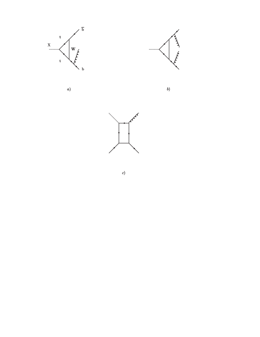
Figure 9: Example of diagrams contributing to ${}{{}{{{{{\mathrm{{{}{}{{X}}\mspace{-0.6mu}}}}}}}}}\to{}{}{{}{{}{{{{{\mathrm{{{}{}{{\overline{{}{{}{{{{{\mathrm{{{}{}{{b}}\mspace{-0.6mu}}}}}}}}}}}_{{\mspace{1.0mu}}}^{\mspace{1.0mu}{{\raisebox{-1.65764pt}{{${{{\scriptstyle{{{{{\mathrm{{}}}}}}}}}}$}}}}}}\mspace{-0.6mu}}}}}}}}}}{}{{}{{{{{\mathrm{{{}{}{{b}}\mspace{-0.6mu}}}}}}}}}{}{{}{{{{{\mathrm{{{}{}{{g}}\mspace{-0.6mu}}}}}}}}}$ and ${}{{}{{{{{\mathrm{{{}{}{{X}}\mspace{-0.6mu}}}}}}}}}\to{}{}{{}{{}{{{{{\mathrm{{{}{}{{\overline{{}{{}{{{{{\mathrm{{{}{}{{b}}\mspace{-0.6mu}}}}}}}}}}}_{{\mspace{1.0mu}}}^{\mspace{1.0mu}{{\raisebox{-1.65764pt}{{${{{\scriptstyle{{{{{\mathrm{{}}}}}}}}}}$}}}}}}\mspace{-0.6mu}}}}}}}}}}{}{{}{{{{{\mathrm{{{}{}{{b}}\mspace{-0.6mu}}}}}}}}}{}{{}{{{{{\mathrm{{{}{}{{g}}\mspace{-0.6mu}}}}}}}}}{}{{}{{{{{\mathrm{{{}{}{{g}}\mspace{-0.6mu}}}}}}}}}$.

Consider now the process ${}{{}{{{{{\mathrm{{{}{}{{X}}\mspace{-0.6mu}}}}}}}}}\to{}{}{{}{{}{{{{{\mathrm{{{}{}{{\overline{{}{{}{{{{{\mathrm{{{}{}{{b}}\mspace{-0.6mu}}}}}}}}}}}_{{\mspace{1.0mu}}}^{\mspace{1.0mu}{{\raisebox{-1.65764pt}{{${{{\scriptstyle{{{{{\mathrm{{}}}}}}}}}}$}}}}}}\mspace{-0.6mu}}}}}}}}}}{}{{}{{{{{\mathrm{{{}{}{{b}}\mspace{-0.6mu}}}}}}}}}{}{{}{{{{{\mathrm{{{}{}{{g}}\mspace{-0.6mu}}}}}}}}}{}{{}{{{{{\mathrm{{{}{}{{g}}\mspace{-0.6mu}}}}}}}}}$, the double gluon emission (e.g. diagram b) in Figure 9). Also in this case there is a physical-region AT as illustrated in Figure 10 where we show ${\mathrm{M}}({}{}{{}{{}{{{{{\mathrm{{{}{}{{\overline{{}{{}{{{{{\mathrm{{{}{}{{b}}\mspace{-0.6mu}}}}}}}}}}}_{{\mspace{1.0mu}}}^{\mspace{1.0mu}{{\raisebox{-1.65764pt}{{${{{\scriptstyle{{{{{\mathrm{{}}}}}}}}}}$}}}}}}\mspace{-0.6mu}}}}}}}}}}{}{{}{{{{{\mathrm{{{}{}{{g}}\mspace{-0.6mu}}}}}}}}})$ as a function of ${\mathrm{M}}({}{{}{{{{{\mathrm{{{}{}{{b}}\mspace{-0.6mu}}}}}}}}}{}{{}{{{{{\mathrm{{{}{}{{g}}\mspace{-0.6mu}}}}}}}}})$ at the AT; as expected, one of the invariant masses should be above $m_{{}{{}{{{{{\mathrm{{{}{}{{t}}\mspace{-0.6mu}}}}}}}}}}+{\mathrm{M}}_{{\scriptscriptstyle{{}{{}{{{{{\mathrm{{{}{}{{W}}\mspace{-0.6mu}}}}}}}}}}}}$ with the other below $m_{{}{{}{{{{{\mathrm{{{}{}{{t}}\mspace{-0.6mu}}}}}}}}}}-{\mathrm{M}}_{{\scriptscriptstyle{{}{{}{{{{{\mathrm{{{}{}{{W}}\mspace{-0.6mu}}}}}}}}}}}}$. It is worth noting that even in this case there is only a small window above $\sqrt{s}=2\,m_{{}{{}{{{{{\mathrm{{{}{}{{t}}\mspace{-0.6mu}}}}}}}}}}$ where the AT shows up, as illustrated by the red curve in Figure 10 which corresponds to $360~{}\text{GeV}$. The physical-region AT disappears around $\sqrt{s}=370~{}\text{GeV}$.

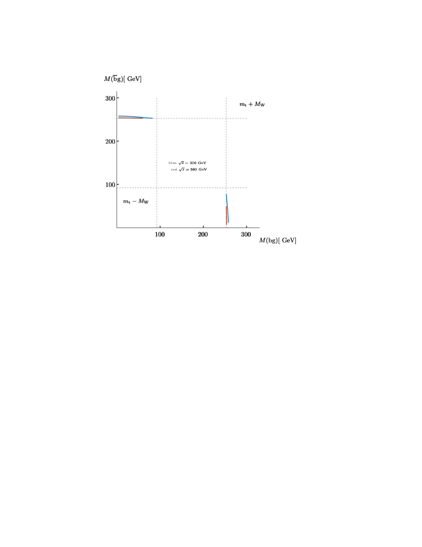
Figure 10: Anomalous threshold in ${}{{}{{{{{\mathrm{{{}{}{{X}}\mspace{-0.6mu}}}}}}}}}\to{}{}{{}{{}{{{{{\mathrm{{{}{}{{\overline{{}{{}{{{{{\mathrm{{{}{}{{b}}\mspace{-0.6mu}}}}}}}}}}}_{{\mspace{1.0mu}}}^{\mspace{1.0mu}{{\raisebox{-1.65764pt}{{${{{\scriptstyle{{{{{\mathrm{{}}}}}}}}}}$}}}}}}\mspace{-0.6mu}}}}}}}}}}{}{{}{{{{{\mathrm{{{}{}{{b}}\mspace{-0.6mu}}}}}}}}}{}{{}{{{{{\mathrm{{{}{}{{g}}\mspace{-0.6mu}}}}}}}}}{}{{}{{{{{\mathrm{{{}{}{{g}}\mspace{-0.6mu}}}}}}}}}$.

However, above $370~{}\text{GeV}$ Peierls zeros start to appear, e.g. at $\sqrt{s}=370~{}\text{GeV}$ the zero corresponds to one invariant mass of $110.36~{}\text{GeV}$ with the other at $200.25~{}\text{GeV}$. At $\sqrt{s}=512~{}\text{GeV}$ the values are $9.73~{}\text{GeV}$ and $245.63~{}\text{GeV}$; above this value the two invariant masses are outside the physical region.

The same line of argument applies to other processes, e.g. ${}{{}{{{{{\mathrm{{{}{}{{g}}\mspace{-0.6mu}}}}}}}}}{}{{}{{{{{\mathrm{{{}{}{{g}}\mspace{-0.6mu}}}}}}}}}\to{}{}{{}{{}{{{{{\mathrm{{{}{}{{\overline{{}{{}{{{{{\mathrm{{{}{}{{b}}\mspace{-0.6mu}}}}}}}}}}}_{{\mspace{1.0mu}}}^{\mspace{1.0mu}{{\raisebox{-1.65764pt}{{${{{\scriptstyle{{{{{\mathrm{{}}}}}}}}}}$}}}}}}\mspace{-0.6mu}}}}}}}}}}{}{{}{{{{{\mathrm{{{}{}{{b}}\mspace{-0.6mu}}}}}}}}}{}{{}{{{{{\mathrm{{{}{}{{g}}\mspace{-0.6mu}}}}}}}}}$ and ${}{{}{{{{{\mathrm{{{}{}{{g}}\mspace{-0.6mu}}}}}}}}}{}{{}{{{{{\mathrm{{{}{}{{g}}\mspace{-0.6mu}}}}}}}}}\to{}{}{{}{{}{{{{{\mathrm{{{}{}{{\overline{{}{{}{{{{{\mathrm{{{}{}{{b}}\mspace{-0.6mu}}}}}}}}}}}_{{\mspace{1.0mu}}}^{\mspace{1.0mu}{{\raisebox{-1.65764pt}{{${{{\scriptstyle{{{{{\mathrm{{}}}}}}}}}}$}}}}}}\mspace{-0.6mu}}}}}}}}}}{}{{}{{{{{\mathrm{{{}{}{{b}}\mspace{-0.6mu}}}}}}}}}{}{{}{{{{{\mathrm{{{}{}{{g}}\mspace{-0.6mu}}}}}}}}}{}{{}{{{{{\mathrm{{{}{}{{g}}\mspace{-0.6mu}}}}}}}}}$ (also to a ${}{}{{}{{}{{{{{\mathrm{{{}{}{{\overline{{}{{}{{{{{\mathrm{{{}{}{{q}}\mspace{-0.6mu}}}}}}}}}}}_{{\mspace{1.0mu}}}^{\mspace{1.0mu}{{\raisebox{-1.65764pt}{{${{{\scriptstyle{{{{{\mathrm{{}}}}}}}}}}$}}}}}}\mspace{-0.6mu}}}}}}}}}}{}{{}{{{{{\mathrm{{{}{}{{q}}\mspace{-0.6mu}}}}}}}}}$ initial state). Let us consider ${}{{}{{{{{\mathrm{{{}{}{{H}}\mspace{-0.6mu}}}}}}}}}^{*}\to{}{}{{}{{}{{{{{\mathrm{{{}{}{{\overline{{}{{}{{{{{\mathrm{{{}{}{{b}}\mspace{-0.6mu}}}}}}}}}}}_{{\mspace{1.0mu}}}^{\mspace{1.0mu}{{\raisebox{-1.65764pt}{{${{{\scriptstyle{{{{{\mathrm{{}}}}}}}}}}$}}}}}}\mspace{-0.6mu}}}}}}}}}}{}{{}{{{{{\mathrm{{{}{}{{b}}\mspace{-0.6mu}}}}}}}}}{}{{}{{{{{\mathrm{{{}{}{{g}}\mspace{-0.6mu}}}}}}}}}$ with an off-shell Higgs boson: we find the following pattern for the amplitude,

$${\mathrm{A}}_{\mathrm{\scriptscriptstyle{LO}}}={\mathrm{A}}^{(1)}_{\mathrm{\scriptscriptstyle{LO}}}\,m_{{}{{}{{{{{\mathrm{{{}{}{{b}}\mspace{-0.6mu}}}}}}}}}}+{\cal O}(m^{2}_{{}{{}{{{{{\mathrm{{{}{}{{b}}\mspace{-0.6mu}}}}}}}}}})\,,\qquad{\mathrm{A}}_{\mathrm{\scriptscriptstyle{NLO}}}={\mathrm{A}}^{(0)}_{\mathrm{\scriptscriptstyle{NLO}}}+{\mathrm{A}}^{(1)}_{\mathrm{\scriptscriptstyle{NLO}}}\,m_{{}{{}{{{{{\mathrm{{{}{}{{b}}\mspace{-0.6mu}}}}}}}}}}+{\cal O}(m^{2}_{{}{{}{{{{{\mathrm{{{}{}{{b}}\mspace{-0.6mu}}}}}}}}}})\,\,.$$ (49)

Therefore, $\mid{\mathrm{A}}\mid^{2}$ is ${\cal O}(m^{2}_{{}{{}{{{{{\mathrm{{{}{}{{b}}\mspace{-0.6mu}}}}}}}}}})$ at LO; there is no interference between ${\mathrm{A}}^{(1)}_{\mathrm{\scriptscriptstyle{LO}}}$ and ${\mathrm{A}}^{(0)}_{\mathrm{\scriptscriptstyle{NLO}}}$ so that the interference (NLO) is also ${\cal O}(m^{2}_{{}{{}{{{{{\mathrm{{{}{}{{b}}\mspace{-0.6mu}}}}}}}}}})$. Since ${\mathrm{A}}_{\mathrm{\scriptscriptstyle{NLO}}}$ contains ${\mathrm{A}}^{\mathrm{\scriptscriptstyle{AT}}}_{\mathrm{\scriptscriptstyle{NLO}}}$ we can include an additional (NNLO) term given by the square of ${\mathrm{A}}^{(0)}_{\mathrm{\scriptscriptstyle{NLO}}}$. Taking into account the logarithmic nature of the AT, the suppression factor $1/(16\,\pi^{2})$ for the loop and the value of the ${}{{}{{{{{\mathrm{{{}{}{{b}}\mspace{-0.6mu}}}}}}}}}\,$-quark mass we do not find any significant effect due to the AT. The process ${}{{}{{{{{\mathrm{{{}{}{{H}}\mspace{-0.6mu}}}}}}}}}^{*}(P)\to{}{{}{{{{{\mathrm{{{}{}{{b}}\mspace{-0.6mu}}}}}}}}}(q_{1})+{}{}{{}{{}{{{{{\mathrm{{{}{}{{\overline{{}{{}{{{{{\mathrm{{{}{}{{b}}\mspace{-0.6mu}}}}}}}}}}}_{{\mspace{1.0mu}}}^{\mspace{1.0mu}{{\raisebox{-1.65764pt}{{${{{\scriptstyle{{{{{\mathrm{{}}}}}}}}}}$}}}}}}\mspace{-0.6mu}}}}}}}}}}(q_{2})+{}{{}{{{{{\mathrm{{{}{}{{g}}\mspace{-0.6mu}}}}}}}}}(q_{3})$, with $P^{2}=-s$ is described by two invariants,

$$s_{1}=-(P-q_{1})^{2}\,,\qquad u_{1}=-(P-q_{2})^{2}\,,$$ (50)

with the following boundaries

$$m^{2}_{{}{{}{{{{{\mathrm{{{}{}{{b}}\mspace{-0.6mu}}}}}}}}}}\leq s_{1}\leq(\sqrt{s}-m_{{}{{}{{{{{\mathrm{{{}{}{{b}}\mspace{-0.6mu}}}}}}}}}})^{2}\,,\qquad u_{1-}\leq u_{1}\leq u_{1+}\,,$$ (51)

where the limits for $u_{1}$ are

$$u_{1\pm}=s+m^{2}_{{}{{}{{{{{\mathrm{{{}{}{{b}}\mspace{-0.6mu}}}}}}}}}}-\frac{1}{2\,s_{1}}\,(s_{1}+m^{2}_{{}{{}{{{{{\mathrm{{{}{}{{b}}\mspace{-0.6mu}}}}}}}}}})\,(s+s_{1}-m^{2}_{{}{{}{{{{{\mathrm{{{}{}{{b}}\mspace{-0.6mu}}}}}}}}}})\pm\frac{1}{2\,s_{1}}\,\lambda^{1/2}(s_{1}\,,\,m^{2}_{{}{{}{{{{{\mathrm{{{}{}{{b}}\mspace{-0.6mu}}}}}}}}}}\,,\,0)\,\lambda^{1/2}(s\,,\,s_{1}\,,\,m^{2}_{{}{{}{{{{{\mathrm{{{}{}{{b}}\mspace{-0.6mu}}}}}}}}}})\,\,.$$ (52)

After inserting the relevant parts of the one-loop corrections we obtain the percentage AT corrections to the pseudo-observable $d\Gamma({}{{}{{{{{\mathrm{{{}{}{{H}}\mspace{-0.6mu}}}}}}}}}^{*}\to{}{}{{}{{}{{{{{\mathrm{{{}{}{{\overline{{}{{}{{{{{\mathrm{{{}{}{{b}}\mspace{-0.6mu}}}}}}}}}}}_{{\mspace{1.0mu}}}^{\mspace{1.0mu}{{\raisebox{-1.65764pt}{{${{{\scriptstyle{{{{{\mathrm{{}}}}}}}}}}$}}}}}}\mspace{-0.6mu}}}}}}}}}}{}{{}{{{{{\mathrm{{{}{}{{b}}\mspace{-0.6mu}}}}}}}}}{}{{}{{{{{\mathrm{{{}{}{{g}}\mspace{-0.6mu}}}}}}}}})/d{\mathrm{M}}({}{{}{{{{{\mathrm{{{}{}{{b}}\mspace{-0.6mu}}}}}}}}}{}{{}{{{{{\mathrm{{{}{}{{g}}\mspace{-0.6mu}}}}}}}}})$, i.e. $\delta^{\mathrm{\scriptscriptstyle{AT}}}_{\mathrm{\scriptscriptstyle{NLO}}\,,\,\mathrm{\scriptscriptstyle{NNLO}}}$. For $\sqrt{s}=350~{}\text{GeV}$ the AT is at $\sqrt{s_{1}}={\mathrm{M}}({}{{}{{{{{\mathrm{{{}{}{{b}}\mspace{-0.6mu}}}}}}}}}{}{{}{{{{{\mathrm{{{}{}{{g}}\mspace{-0.6mu}}}}}}}}})\approx 257.82~{}\text{GeV}$. After imposing a cut of $10~{}\text{GeV}$ on all final state invariant masses we obtain the result shown in the left panel of Figure 11; NLO and NNLO are indistinguishable. The AT effect is very small and corresponds to a change in the curvature of $\delta^{\mathrm{\scriptscriptstyle{AT}}}$.

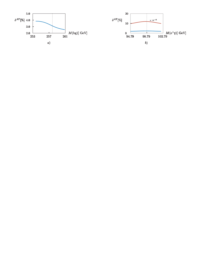
Figure 11: AT induced radiative corrections for a) ${}{{}{{{{{\mathrm{{{}{}{{H}}\mspace{-0.6mu}}}}}}}}}^{*}\to{}{}{{}{{}{{{{{\mathrm{{{}{}{{\overline{{}{{}{{{{{\mathrm{{{}{}{{b}}\mspace{-0.6mu}}}}}}}}}}}_{{\mspace{1.0mu}}}^{\mspace{1.0mu}{{\raisebox{-1.65764pt}{{${{{\scriptstyle{{{{{\mathrm{{}}}}}}}}}}$}}}}}}\mspace{-0.6mu}}}}}}}}}}{}{{}{{{{{\mathrm{{{}{}{{b}}\mspace{-0.6mu}}}}}}}}}{}{{}{{{{{\mathrm{{{}{}{{g}}\mspace{-0.6mu}}}}}}}}}$ and b) ${}{{}{{{{{\mathrm{{{}{}{{H}}\mspace{-0.6mu}}}}}}}}}^{*}\to{}{{}{{{{{\mathrm{{{}{}{{{}{{}{{{{{\mathrm{{{}{}{{e}}\mspace{-0.6mu}}}}}}}}}}^{+}}\mspace{-0.6mu}}}}}}}}}{}{{}{{{{{\mathrm{{{}{}{{{}{{}{{{{{\mathrm{{{}{}{{e}}\mspace{-0.6mu}}}}}}}}}}^{-}}\mspace{-0.6mu}}}}}}}}}{}{{}{{{{{\mathrm{{{}{}{}\mspace{-0.6mu}}}}}}}}}$. The ${}{{}{{{{{\mathrm{{{}{}{{H}}\mspace{-0.6mu}}}}}}}}}$ virtuality is a) $\sqrt{s}=350~{}\text{GeV}$ and b) $\sqrt{s}=170~{}\text{GeV}$.

${}{{}{{{{{\mathrm{{{}{}{{{}{{}{{{{{\mathrm{{{}{}{{e}}\mspace{-0.6mu}}}}}}}}}}^{+}}\mspace{-0.6mu}}}}}}}}}{}{{}{{{{{\mathrm{{{}{}{{{}{{}{{{{{\mathrm{{{}{}{{e}}\mspace{-0.6mu}}}}}}}}}}^{-}}\mspace{-0.6mu}}}}}}}}}{}{{}{{{{{\mathrm{{{}{}{}\mspace{-0.6mu}}}}}}}}}$ final state

For this process we can have a ${}{{}{{{{{\mathrm{{{}{}{{W}}\mspace{-0.6mu}}}}}}}}}{-}{}{{}{{{{{\mathrm{{{}{}{}\mspace{-0.6mu}}}}}}}}}{-}{}{{}{{{{{\mathrm{{{}{}{{W}}\mspace{-0.6mu}}}}}}}}}$ triangle: in this case $\sqrt{s}$ must be above $2\,M_{{}{{}{{{{{\mathrm{{{}{}{{W}}\mspace{-0.6mu}}}}}}}}}}$ for a physical-region AT, as dictated by the Coleman-Norton theorem. The physical-region AT starts at $\sqrt{s}=161.05~{}\text{GeV}$ with ${\mathrm{M}}({}{{}{{{{{\mathrm{{{}{}{{{}{{}{{{{{\mathrm{{{}{}{{e}}\mspace{-0.6mu}}}}}}}}}}^{+}}\mspace{-0.6mu}}}}}}}}}{}{{}{{{{{\mathrm{{{}{}{}\mspace{-0.6mu}}}}}}}}})=110.64~{}\text{GeV}$ and approaches ${\mathrm{M}}({}{{}{{{{{\mathrm{{{}{}{{{}{{}{{{{{\mathrm{{{}{}{{e}}\mspace{-0.6mu}}}}}}}}}}^{+}}\mspace{-0.6mu}}}}}}}}}{}{{}{{{{{\mathrm{{{}{}{}\mspace{-0.6mu}}}}}}}}})=M_{{}{{}{{{{{\mathrm{{{}{}{{W}}\mspace{-0.6mu}}}}}}}}}}$ for very large values of $\sqrt{s}$. It is worth noting that all diagrams contributing to ${}{{}{{{{{\mathrm{{{}{}{{H}}\mspace{-0.6mu}}}}}}}}}^{*}\to{}{{}{{{{{\mathrm{{{}{}{{Z}}\mspace{-0.6mu}}}}}}}}}(\to{}{{}{{{{{\mathrm{{{}{}{{{}{{}{{{{{\mathrm{{{}{}{{e}}\mspace{-0.6mu}}}}}}}}}}^{+}}\mspace{-0.6mu}}}}}}}}}{}{{}{{{{{\mathrm{{{}{}{{{}{{}{{{{{\mathrm{{{}{}{{e}}\mspace{-0.6mu}}}}}}}}}}^{-}}\mspace{-0.6mu}}}}}}}}})+{}{{}{{{{{\mathrm{{{}{}{}\mspace{-0.6mu}}}}}}}}}$ do not show an AT. For this process, due to the small value of $m_{{}{{}{{{{{\mathrm{{{}{}{{e}}\mspace{-0.6mu}}}}}}}}}}$ the inclusion of NNLO terms changes drastically the result as shown in the right panel of Figure 11, i.e. the NNLO contribution is six orders of magnitude larger than the LO term at $\sqrt{s}=170~{}\text{GeV}$. Here the red curve corresponds to no cut while the red one corresponds to a cut of $10~{}\text{GeV}$ on all final state invariant masses. In this case $\delta^{\mathrm{\scriptscriptstyle{AT}}}$ shows a peak at the AT.

We can also have a ${}{{}{{{{{\mathrm{{{}{}{{Z}}\mspace{-0.6mu}}}}}}}}}{-}{}{{}{{{{{\mathrm{{{}{}{{e}}\mspace{-0.6mu}}}}}}}}}{-}{}{{}{{{{{\mathrm{{{}{}{{Z}}\mspace{-0.6mu}}}}}}}}}$ triangle: in this case $\sqrt{s}$ must be above $2\,M_{{}{{}{{{{{\mathrm{{{}{}{{Z}}\mspace{-0.6mu}}}}}}}}}}$. The physical-region AT starts at $\sqrt{s}=182.38~{}\text{GeV}$ with ${\mathrm{M}}({}{{}{{{{{\mathrm{{{}{}{{{}{{}{{{{{\mathrm{{{}{}{{e}}\mspace{-0.6mu}}}}}}}}}}^{+}}\mspace{-0.6mu}}}}}}}}}{}{{}{{{{{\mathrm{{{}{}{}\mspace{-0.6mu}}}}}}}}})=128.96~{}\text{GeV}$ and approaches ${\mathrm{M}}({}{{}{{{{{\mathrm{{{}{}{{{}{{}{{{{{\mathrm{{{}{}{{e}}\mspace{-0.6mu}}}}}}}}}}^{+}}\mspace{-0.6mu}}}}}}}}}{}{{}{{{{{\mathrm{{{}{}{}\mspace{-0.6mu}}}}}}}}})=M_{{}{{}{{{{{\mathrm{{{}{}{{Z}}\mspace{-0.6mu}}}}}}}}}}$ for very large values of $\sqrt{s}$.

${}{{}{{{{{\mathrm{{{}{}{{{}{{}{{{{{\mathrm{{{}{}{{e}}\mspace{-0.6mu}}}}}}}}}}^{+}}\mspace{-0.6mu}}}}}}}}}{}{{}{{{{{\mathrm{{{}{}{{{}{{}{{{{{\mathrm{{{}{}{{e}}\mspace{-0.6mu}}}}}}}}}}^{-}}\mspace{-0.6mu}}}}}}}}}$ colliders

It is worth noting that the same qualitative behavior will be found for

$${}{{}{{{{{\mathrm{{{}{}{{{}{{}{{{{{\mathrm{{{}{}{{e}}\mspace{-0.6mu}}}}}}}}}}^{+}}\mspace{-0.6mu}}}}}}}}}+{}{{}{{{{{\mathrm{{{}{}{{{}{{}{{{{{\mathrm{{{}{}{{e}}\mspace{-0.6mu}}}}}}}}}}^{-}}\mspace{-0.6mu}}}}}}}}}\to{}{{}{{{{{\mathrm{{{}{}{{Z}}\mspace{-0.6mu}}}}}}}}}/{}{{}{{{{{\mathrm{{{}{}{}\mspace{-0.6mu}}}}}}}}}\to{}{}{{}{{}{{{{{\mathrm{{{}{}{{\overline{{}{{}{{{{{\mathrm{{{}{}{{b}}\mspace{-0.6mu}}}}}}}}}}}_{{\mspace{1.0mu}}}^{\mspace{1.0mu}{{\raisebox{-1.65764pt}{{${{{\scriptstyle{{{{{\mathrm{{}}}}}}}}}}$}}}}}}\mspace{-0.6mu}}}}}}}}}}+{}{{}{{{{{\mathrm{{{}{}{{b}}\mspace{-0.6mu}}}}}}}}}+{}{{}{{{{{\mathrm{{{}{}{{g}}\mspace{-0.6mu}}}}}}}}}\,,\qquad{}{{}{{{{{\mathrm{{{}{}{{{}{{}{{{{{\mathrm{{{}{}{{e}}\mspace{-0.6mu}}}}}}}}}}^{+}}\mspace{-0.6mu}}}}}}}}}+{}{{}{{{{{\mathrm{{{}{}{{{}{{}{{{{{\mathrm{{{}{}{{e}}\mspace{-0.6mu}}}}}}}}}}^{-}}\mspace{-0.6mu}}}}}}}}}\to{}{{}{{{{{\mathrm{{{}{}{{Z}}\mspace{-0.6mu}}}}}}}}}/{}{{}{{{{{\mathrm{{{}{}{}\mspace{-0.6mu}}}}}}}}}\to{}{}{{}{{}{{{{{\mathrm{{{}{}{{\overline{{}{{}{{{{{\mathrm{{{}{}{{f}}\mspace{-0.6mu}}}}}}}}}}}_{{\mspace{1.0mu}}}^{\mspace{1.0mu}{{\raisebox{-1.65764pt}{{${{{\scriptstyle{{{{{\mathrm{{}}}}}}}}}}$}}}}}}\mspace{-0.6mu}}}}}}}}}}+{}{{}{{{{{\mathrm{{{}{}{{f}}\mspace{-0.6mu}}}}}}}}}+{}{{}{{{{{\mathrm{{{}{}{}\mspace{-0.6mu}}}}}}}}}\,,$$ (53)

and also for ${}{{}{{{{{\mathrm{{{}{}{{{}{{}{{{{{\mathrm{{{}{}{{e}}\mspace{-0.6mu}}}}}}}}}}^{+}}\mspace{-0.6mu}}}}}}}}}+{}{{}{{{{{\mathrm{{{}{}{{{}{{}{{{{{\mathrm{{{}{}{{e}}\mspace{-0.6mu}}}}}}}}}}^{-}}\mspace{-0.6mu}}}}}}}}}\to{}{}{{}{{}{{{{{\mathrm{{{}{}{{\overline{{}{{}{{{{{\mathrm{{{}{}{{b}}\mspace{-0.6mu}}}}}}}}}}}_{{\mspace{1.0mu}}}^{\mspace{1.0mu}{{\raisebox{-1.65764pt}{{${{{\scriptstyle{{{{{\mathrm{{}}}}}}}}}}$}}}}}}\mspace{-0.6mu}}}}}}}}}}+{}{{}{{{{{\mathrm{{{}{}{{b}}\mspace{-0.6mu}}}}}}}}}+{}{{}{{{{{\mathrm{{{}{}{}\mspace{-0.6mu}}}}}}}}}+{}{{}{{{{{\mathrm{{{}{}{}\mspace{-0.6mu}}}}}}}}}$, an irreducible background process in measuring the ${}{{}{{{{{\mathrm{{{}{}{{H}}\mspace{-0.6mu}}}}}}}}}\to{}{{}{{{{{\mathrm{{{}{}{}\mspace{-0.6mu}}}}}}}}}{}{{}{{{{{\mathrm{{{}{}{}\mspace{-0.6mu}}}}}}}}}$ decay at a linear collider.

5 Box diagrams

Consider the diagram of Figure 12 where $Q=q_{1}+q_{2}+q_{3}$, with $Q^{2}=-s$ and $q^{2}_{i}=-{\mathrm{M}}^{2}_{i}$. The physical region is defined in terms of invariants [91],

$$s_{1}=-(Q-q_{1})^{2}\,,\quad u_{1}=-(Q-q_{2})^{2}\,\,.$$ (54)

We derive

$$({\mathrm{M}}_{2}+{\mathrm{M}}_{3})^{2}\leq s_{1}\leq(\sqrt{s}-{\mathrm{M}}_{1})^{2}\,,\qquad u_{1-}\leq u_{1}\leq u_{1+}\,,$$ (55)

where the limits for $u_{1}$ are

$$u_{1\pm}=s+{\mathrm{M}}^{2}_{2}-\frac{1}{2\,s_{1}}\,\Bigl{[}(s_{1}+{\mathrm{M}}^{2}_{2}-{\mathrm{M}}^{2}_{3})\,(s+s_{1}-{\mathrm{M}}^{2}_{1})\mp\lambda^{1/2}(s_{1}\,,\,{\mathrm{M}}^{2}_{2}\,,\,{\mathrm{M}}^{2}_{3})\,\lambda^{1/2}(s\,,\,s_{1}\,,\,{\mathrm{M}}^{2}_{1})\Bigr{]}\,\,.$$ (56)

Therefore, we are interested in the process ${}{{}{{{{{\mathrm{{{}{}{{g}}\mspace{-0.6mu}}}}}}}}}{}{{}{{{{{\mathrm{{{}{}{{g}}\mspace{-0.6mu}}}}}}}}}\to{}{}{{}{{}{{{{{\mathrm{{{}{}{{\overline{{}{{}{{{{{\mathrm{{{}{}{{b}}\mspace{-0.6mu}}}}}}}}}}}_{{\mspace{1.0mu}}}^{\mspace{1.0mu}{{\raisebox{-1.65764pt}{{${{{\scriptstyle{{{{{\mathrm{{}}}}}}}}}}$}}}}}}\mspace{-0.6mu}}}}}}}}}}{}{{}{{{{{\mathrm{{{}{}{{b}}\mspace{-0.6mu}}}}}}}}}{}{{}{{{{{\mathrm{{{}{}{{H}}\mspace{-0.6mu}}}}}}}}}$ where ${}{{}{{{{{\mathrm{{{}{}{{H}}\mspace{-0.6mu}}}}}}}}}$ can be an off-shell Higgs boson of the SM or some, on-shell, heavy Higgs boson present in some BSM model. Another case of interest is represented by ${}{{}{{{{{\mathrm{{{}{}{{g}}\mspace{-0.6mu}}}}}}}}}{}{{}{{{{{\mathrm{{{}{}{{g}}\mspace{-0.6mu}}}}}}}}}\to{}{}{{}{{}{{{{{\mathrm{{{}{}{{\overline{{}{{}{{{{{\mathrm{{{}{}{{b}}\mspace{-0.6mu}}}}}}}}}}}_{{\mspace{1.0mu}}}^{\mspace{1.0mu}{{\raisebox{-1.65764pt}{{${{{\scriptstyle{{{{{\mathrm{{}}}}}}}}}}$}}}}}}\mspace{-0.6mu}}}}}}}}}}{}{{}{{{{{\mathrm{{{}{}{{b}}\mspace{-0.6mu}}}}}}}}}{}{{}{{{{{\mathrm{{{}{}{{H}}\mspace{-0.6mu}}}}}}}}}{}{{}{{{{{\mathrm{{{}{}{{H}}\mspace{-0.6mu}}}}}}}}}$; here the two SM Higgs bosons are on shell, therefore $q_{2}=q_{21}+q_{22}$ with $q^{2}_{2i}=-{\mathrm{M}}^{2}_{{\scriptscriptstyle{{}{{}{{{{{\mathrm{{{}{}{{H}}\mspace{-0.6mu}}}}}}}}}}}}$ and ${\mathrm{M}}_{2}$ is the invariant mass of the ${}{{}{{{{{\mathrm{{{}{}{{H}}\mspace{-0.6mu}}}}}}}}}{}{{}{{{{{\mathrm{{{}{}{{H}}\mspace{-0.6mu}}}}}}}}}$ pair. Using ${\mathrm{M}}_{1,3}=m_{{}{{}{{{{{\mathrm{{{}{}{{b}}\mspace{-0.6mu}}}}}}}}}}$ and ${\mathrm{M}}={\mathrm{M}}_{2}$ we compute the corresponding $\Delta_{4}$ using ${\mathrm{L}}_{4}=m^{2}_{{}{{}{{{{{\mathrm{{{}{}{{t}}\mspace{-0.6mu}}}}}}}}}}$ and

$${\mathrm{G}}_{4}=-\frac{1}{4}\,\left(a\,{\mathrm{M}}^{4}+b\,{\mathrm{M}}^{2}+c\right)\,,$$ (57)

$$a=m^{2}_{{}{{}{{{{{\mathrm{{{}{}{{b}}\mspace{-0.6mu}}}}}}}}}}\,,\quad b=(s-s_{1})\,u_{1}-(2\,s+u_{1})\,m^{2}_{{}{{}{{{{{\mathrm{{{}{}{{b}}\mspace{-0.6mu}}}}}}}}}}\,,\quad c=(s_{1}+u_{1}-s)\,s_{1}\,u_{1}+(s^{2}-s\,u_{1}-2\,s_{1}\,u_{1})\,m^{2}_{{}{{}{{{{{\mathrm{{{}{}{{b}}\mspace{-0.6mu}}}}}}}}}}+u_{1}\,m^{4}_{{}{{}{{{{{\mathrm{{{}{}{{b}}\mspace{-0.6mu}}}}}}}}}}\,\,.$$ (58)

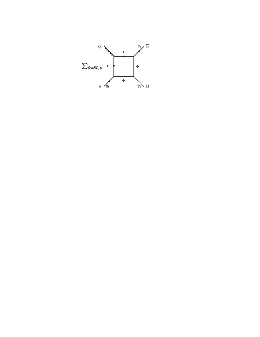
Figure 12: Family a) for ${}{{}{{{{{\mathrm{{{}{}{{g}}\mspace{-0.6mu}}}}}}}}}(Q)\to{}{{}{{{{{\mathrm{{{}{}{{b}}\mspace{-0.6mu}}}}}}}}}(q_{1})+{}{}{{}{{}{{{{{\mathrm{{{}{}{{\overline{{}{{}{{{{{\mathrm{{{}{}{{b}}\mspace{-0.6mu}}}}}}}}}}}_{{\mspace{1.0mu}}}^{\mspace{1.0mu}{{\raisebox{-1.65764pt}{{${{{\scriptstyle{{{{{\mathrm{{}}}}}}}}}}$}}}}}}\mspace{-0.6mu}}}}}}}}}}(q_{3})+{}{{}{{{{{\mathrm{{{}{}{{H}}\mspace{-0.6mu}}}}}}}}}(q_{2})$.

It can be seen that $\Delta_{4}=0$ produces a quadratic equation in ${\mathrm{M}}^{2}$ that can be solved for fixed $s,s_{1},u_{1}$. A scan in the $s_{1}{-}u_{1}$ plane is shown in Figure 13 for $\sqrt{s}=350~{}\text{GeV}$; the blue region shows values for ${\mathrm{M}}^{2}$ which correspond to a physical-region AT, i.e. $\Delta_{4}=0$, ordered values for $X_{i}$ ($0<X_{3}<X_{2}<X_{1}<1$) and a real value for ${\mathrm{M}}$ inside the physical region given in Eq.(55).

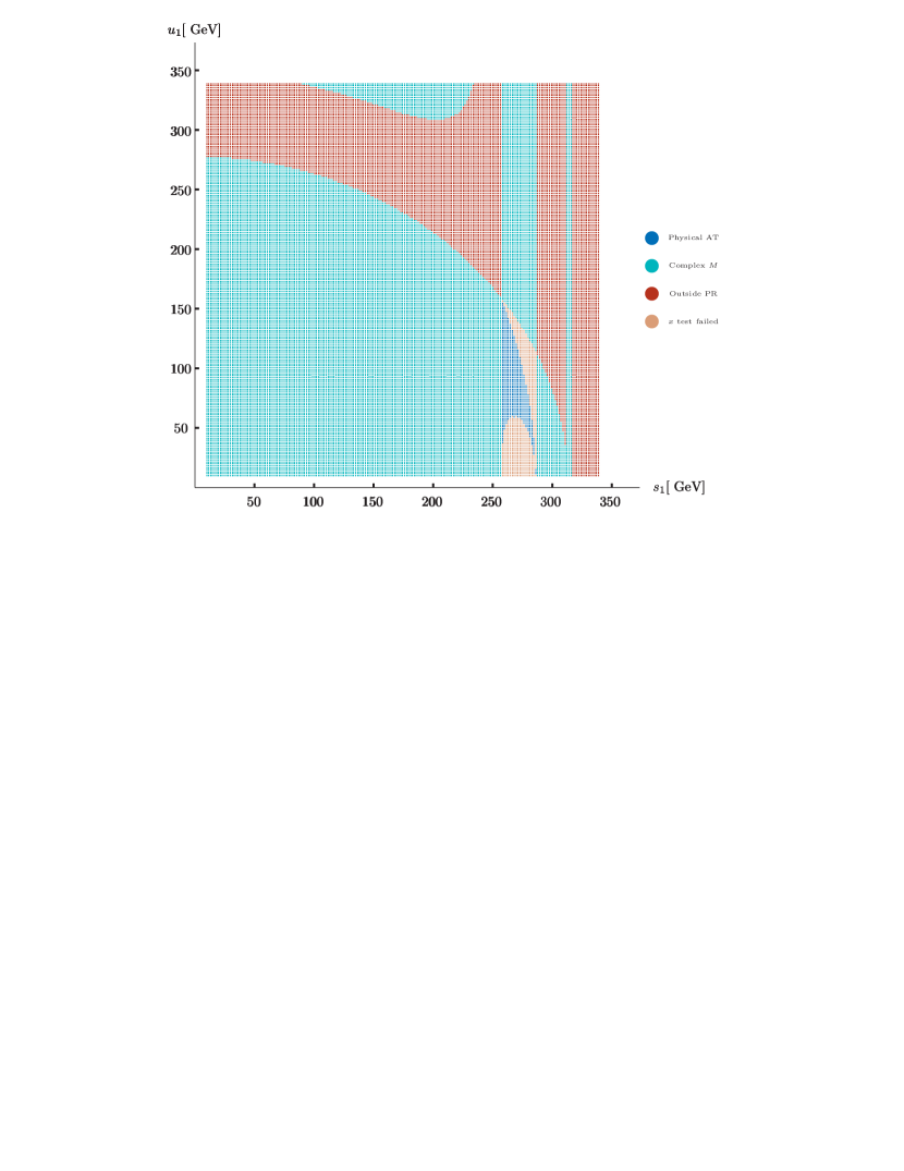
Figure 13: A scan in the $s_{1}{-}u_{1}$ plane searching for a physical-region AT in ${}{{}{{{{{\mathrm{{{}{}{{g}}\mspace{-0.6mu}}}}}}}}}{}{{}{{{{{\mathrm{{{}{}{{g}}\mspace{-0.6mu}}}}}}}}}\to{}{}{{}{{}{{{{{\mathrm{{{}{}{{\overline{{}{{}{{{{{\mathrm{{{}{}{{b}}\mspace{-0.6mu}}}}}}}}}}}_{{\mspace{1.0mu}}}^{\mspace{1.0mu}{{\raisebox{-1.65764pt}{{${{{\scriptstyle{{{{{\mathrm{{}}}}}}}}}}$}}}}}}\mspace{-0.6mu}}}}}}}}}}{}{{}{{{{{\mathrm{{{}{}{{b}}\mspace{-0.6mu}}}}}}}}}{}{{}{{{{{\mathrm{{{}{}{{H}}\mspace{-0.6mu}}}}}}}}}({}{{}{{{{{\mathrm{{{}{}{{H}}\mspace{-0.6mu}}}}}}}}}{}{{}{{{{{\mathrm{{{}{}{{H}}\mspace{-0.6mu}}}}}}}}})$.

Next we introduce complex poles for ${}{{}{{{{{\mathrm{{{}{}{{W}}\mspace{-0.6mu}}}}}}}}}$ and ${}{{}{{{{{\mathrm{{{}{}{{t}}\mspace{-0.6mu}}}}}}}}}$ and look for Peierls zeros. The two equations, $\mathop{\mathrm{Re}}\nolimits\,\Delta_{4}=0$ and $\mathop{\mathrm{Im}}\nolimits\,\Delta_{4}=0$ are quadratic in $u_{1}$ and ${\mathrm{M}}^{2}$ for fixed $s$ and $s_{1}$ generating four solutions. To give an example we fix $\sqrt{s}=350~{}\text{GeV}$ and derive

• one of the solutions for a physical-region AT is $\sqrt{s_{1}}=259.15~{}\text{GeV}$, $\sqrt{u_{1}}=38.05~{}\text{GeV}$ and ${\mathrm{M}}=162.46~{}\text{GeV}$

• for $\sqrt{s_{1}}=259.15~{}\text{GeV}$, one solution returns a negative value for $u_{1}$ and the other three (two are coincident) return ${\mathrm{M}}=172.87~{}\text{GeV},\sqrt{u_{1}}=58.13~{}\text{GeV}$ and ${\mathrm{M}}=191.84~{}\text{GeV},\sqrt{u_{1}}=158.16~{}\text{GeV}$, both outside the physical region.

Any box diagram is decomposed into a box in $6$ dimensions and four triangles: an example is given in Figure 14. As a consequence we have to look not only for the LLS of the box but also for the subleading ones, which are the leading singularities for the triangles.

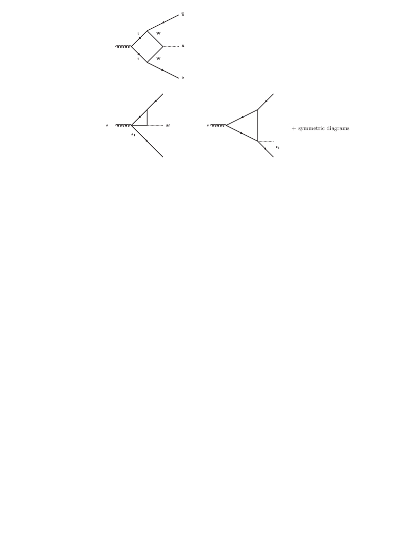
Figure 14: Box diagram producing an AT for ${}{{}{{{{{\mathrm{{{}{}{{g}}\mspace{-0.6mu}}}}}}}}}\to{}{}{{}{{}{{{{{\mathrm{{{}{}{{\overline{{}{{}{{{{{\mathrm{{{}{}{{b}}\mspace{-0.6mu}}}}}}}}}}}_{{\mspace{1.0mu}}}^{\mspace{1.0mu}{{\raisebox{-1.65764pt}{{${{{\scriptstyle{{{{{\mathrm{{}}}}}}}}}}$}}}}}}\mspace{-0.6mu}}}}}}}}}}{}{{}{{{{{\mathrm{{{}{}{{b}}\mspace{-0.6mu}}}}}}}}}{}{{}{{{{{\mathrm{{{}{}{{X}}\mspace{-0.6mu}}}}}}}}}$ where ${}{{}{{{{{\mathrm{{{}{}{{X}}\mspace{-0.6mu}}}}}}}}}$ can be some heavy BSM Higgs boson, an off-shell SM Higgs boson or a pair of two (on-shell) SM Higgs boson. In the second part of the figure we show two of the four triangles obtained by shrinking one line of the box to a point.

Old examples can be found in Ref. [40] for the process ${}{}{{}{{}{{{{{\mathrm{{{}{}{{\overline{p}}_{{\mspace{1.0mu}}}^{\mspace{1.0mu}{{\raisebox{-1.65764pt}{{${{{\scriptstyle{{{{{\mathrm{{}}}}}}}}}}$}}}}}}\mspace{-0.6mu}}}}}}}}}}{}{{}{{{{{\mathrm{{{}{}{{p}}\mspace{-0.6mu}}}}}}}}}\to{}{{}{{{{{\mathrm{{{}{}{{K}}\mspace{-0.6mu}}}}}}}}}{}{{}{{{{{\mathrm{{{}{}{{K}}\mspace{-0.6mu}}}}}}}}}{}{{}{{{{{\mathrm{{{}{}{}\mspace{-0.6mu}}}}}}}}}{}{{}{{{{{\mathrm{{{}{}{}\mspace{-0.6mu}}}}}}}}}$ where peaks were predicted for the amplitude squared in a certain range of the external variables.

We start our analysis by looking at ${}{{}{{{{{\mathrm{{{}{}{{g}}\mspace{-0.6mu}}}}}}}}}(Q)\to{}{{}{{{{{\mathrm{{{}{}{{b}}\mspace{-0.6mu}}}}}}}}}(q_{1})+{}{}{{}{{}{{{{{\mathrm{{{}{}{{\overline{{}{{}{{{{{\mathrm{{{}{}{{b}}\mspace{-0.6mu}}}}}}}}}}}_{{\mspace{1.0mu}}}^{\mspace{1.0mu}{{\raisebox{-1.65764pt}{{${{{\scriptstyle{{{{{\mathrm{{}}}}}}}}}}$}}}}}}\mspace{-0.6mu}}}}}}}}}}(q_{3})+{}{{}{{{{{\mathrm{{{}{}{{X}}\mspace{-0.6mu}}}}}}}}}(q_{2})$ at the point

$${\mathrm{P}}=\{\sqrt{s}=350~{}\text{GeV}\,\,;\,\,\sqrt{s_{1}}=259.15~{}\text{GeV}\,\,;\,\,\sqrt{u_{1}}=155.20~{}\text{GeV}\}\,,$$ (59)

as a function of ${\mathrm{M}}^{2}=-q^{2}_{2}$. It is worth noting that the location of the AT does not depend on the nature of ${}{{}{{{{{\mathrm{{{}{}{{X}}\mspace{-0.6mu}}}}}}}}}$, but its numerical impact on the amplitude does.

For zero widths there is a physical-region AT at ${\mathrm{M}}=187.72~{}\text{GeV}$; the Peierls zeros corresponding to $\sqrt{s_{1}}=259.15~{}\text{GeV}$ are located at $\sqrt{u_{1}}=58.13~{}\text{GeV},{\mathrm{M}}=172.87~{}\text{GeV}$ and $\sqrt{u_{1}}=158.16~{}\text{GeV},{\mathrm{M}}=191.84~{}\text{GeV}$. They are both outside the physical region with the latter close to the boundary $u_{1-}\leq u_{1}\leq u_{1+}$.

In Figure 15 we plot ${\mathrm{L}}(s^{2}\,\mathop{\mathrm{Re}}\nolimits\,{\mathrm{D}}_{0})$ (Eq.(40)) corresponding to ${}{{}{{{{{\mathrm{{{}{}{{g}}\mspace{-0.6mu}}}}}}}}}(Q)\to{}{{}{{{{{\mathrm{{{}{}{{b}}\mspace{-0.6mu}}}}}}}}}(q_{1})+{}{}{{}{{}{{{{{\mathrm{{{}{}{{\overline{{}{{}{{{{{\mathrm{{{}{}{{b}}\mspace{-0.6mu}}}}}}}}}}}_{{\mspace{1.0mu}}}^{\mspace{1.0mu}{{\raisebox{-1.65764pt}{{${{{\scriptstyle{{{{{\mathrm{{}}}}}}}}}}$}}}}}}\mspace{-0.6mu}}}}}}}}}}(q_{3})+{}{{}{{{{{\mathrm{{{}{}{{X}}\mspace{-0.6mu}}}}}}}}}(q_{2})$ at the point of Eq.(59). A blow up of the same figure is shown in Figure 16, including the imaginary part.

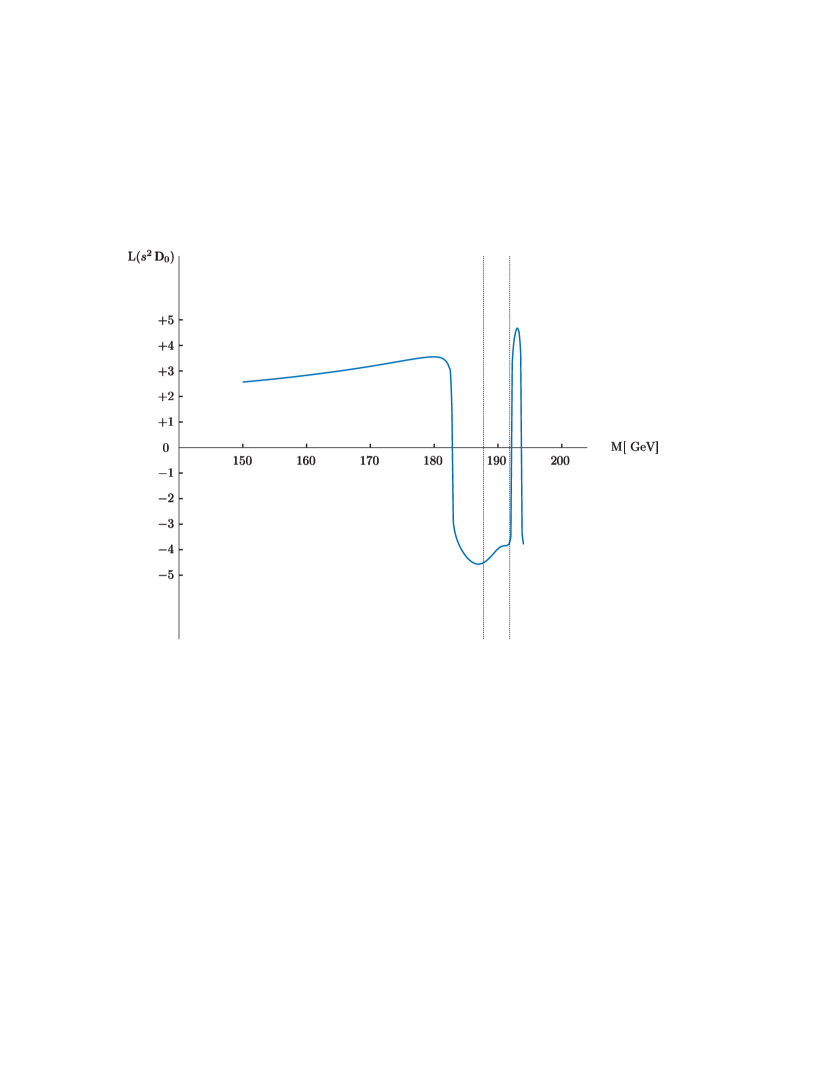
Figure 15: The real part of $s^{2}\,{\mathrm{D}}_{0}$ for ${}{{}{{{{{\mathrm{{{}{}{{g}}\mspace{-0.6mu}}}}}}}}}(Q)\to{}{{}{{{{{\mathrm{{{}{}{{b}}\mspace{-0.6mu}}}}}}}}}(q_{1})+{}{}{{}{{}{{{{{\mathrm{{{}{}{{\overline{{}{{}{{{{{\mathrm{{{}{}{{b}}\mspace{-0.6mu}}}}}}}}}}}_{{\mspace{1.0mu}}}^{\mspace{1.0mu}{{\raisebox{-1.65764pt}{{${{{\scriptstyle{{{{{\mathrm{{}}}}}}}}}}$}}}}}}\mspace{-0.6mu}}}}}}}}}}(q_{3})+{}{{}{{{{{\mathrm{{{}{}{{X}}\mspace{-0.6mu}}}}}}}}}(q_{2})$ at the point of Eq.(59). ${\mathrm{L}}(x)$ is defined in Eq.(40).

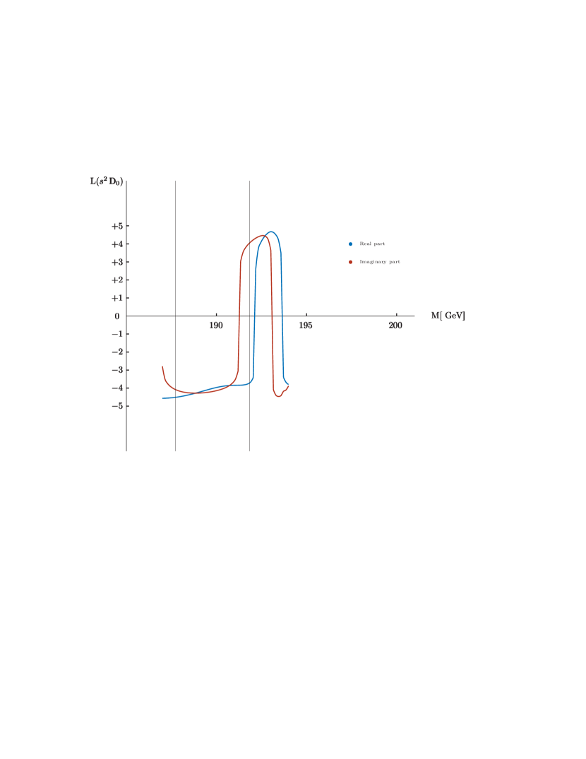
Figure 16: Blow up of Figure 15.

To understand the behavior of ${\mathrm{D}}_{0}$ we split the function as follows: ${\mathrm{V}}(x_{1}\,,\,x_{2}\,,\,x_{3})$ is the quadratic form for the box; introduce triangles

$${\mathrm{T}}=\sum_{i=0}^{3}\,\left(X_{i}-X_{i+1}\right)\,\int\,dS_{2}\,{\mathrm{V}}^{-1}\left(\widehat{i\;i+1}\right)\,,$$ (60)

where $X_{0}=1$, $X_{4}=0$ and $(\widehat{0\;1})=(1\,,\,x_{1}\,,\,x_{2})$ etc. are contractions. Therefore we obtain

$${\mathrm{D}}_{0}(\mathrm{dim}=4)=-\frac{1}{2\,\Delta_{4}}\,\Bigl{[}{\mathrm{D}}_{0}(\mathrm{dim}=6)-{\mathrm{T}}\Bigr{]}=-\frac{1}{2\,\Delta_{4}}\,\Bigl{\{}\frac{3}{2\,\Delta_{4}}\,\Bigl{[}{\mathrm{D}}_{0}(\mathrm{dim}=8)-\frac{1}{2}\,{\mathrm{T}}\Bigr{]}\,-{\mathrm{T}}\Bigr{\}}\,,$$ (61)

and plot

$${\mathrm{D}}_{0}(\mathrm{dim}=4)\,,\quad{\mathrm{D}}^{(6)}_{0}(\mathrm{dim}=4)=-\frac{1}{2\,\Delta_{4}}\,{\mathrm{D}}_{0}(\mathrm{dim}=6)\,,\quad{\mathrm{D}}^{(8)}_{0}(\mathrm{dim}=4)=-\frac{3}{4\,\Delta^{2}_{4}}\,{\mathrm{D}}_{0}(\mathrm{dim}=8)\,,$$ (62)

where the $\mathrm{dim}=8$ part is

$${\mathrm{D}}_{0}(\mathrm{dim}=8)=\int\,dS_{3}\,\Bigl{[}\ln V(x_{1}\,,\,x_{2}\,,\,x_{3})+\frac{2}{3}\Bigr{]}\,\,.$$ (63)

The $3$ components introduced in Eq.(62) are shown in Figure 17 for ${}{{}{{{{{\mathrm{{{}{}{{g}}\mspace{-0.6mu}}}}}}}}}(Q)\to{}{{}{{{{{\mathrm{{{}{}{{b}}\mspace{-0.6mu}}}}}}}}}(q_{1})+{}{}{{}{{}{{{{{\mathrm{{{}{}{{\overline{{}{{}{{{{{\mathrm{{{}{}{{b}}\mspace{-0.6mu}}}}}}}}}}}_{{\mspace{1.0mu}}}^{\mspace{1.0mu}{{\raisebox{-1.65764pt}{{${{{\scriptstyle{{{{{\mathrm{{}}}}}}}}}}$}}}}}}\mspace{-0.6mu}}}}}}}}}}(q_{3})+{}{{}{{{{{\mathrm{{{}{}{{X}}\mspace{-0.6mu}}}}}}}}}(q_{2})$ at the point of Eq.(59).

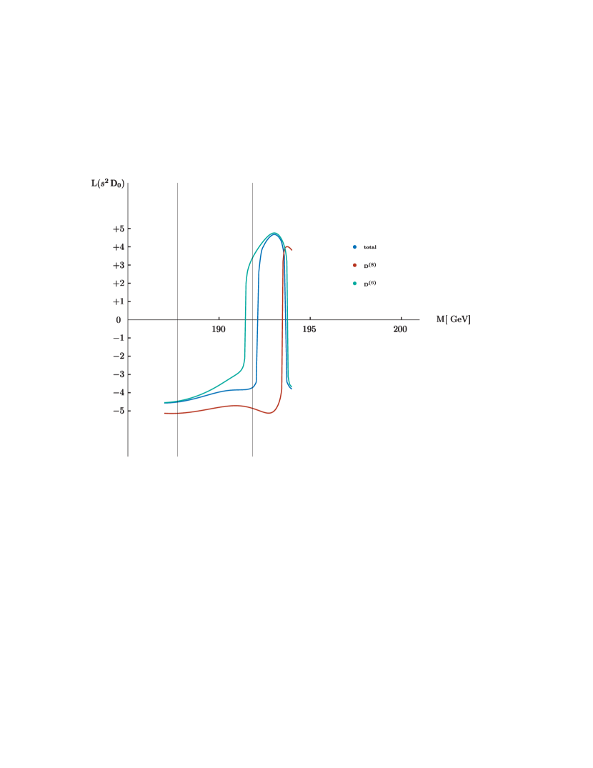
Figure 17: Different components for $\mathop{\mathrm{Re}}\nolimits\,{\mathrm{D}}_{0}$ as explained in Eq.(62).

Finally we introduce

$${\mathrm{I}}_{{\mathrm{D}}_{0}}=\int_{u_{1-}}^{u_{1+}}\,du_{1}\,\mathop{\mathrm{Re}}\nolimits\,{\mathrm{D}}_{0}\,,$$ (64)

where $u_{1\pm}$ are given in Eq.(56). The corresponding function ${\mathrm{L}}(s\,{\mathrm{I}}_{{\mathrm{D}}_{0}})$ (Eq.(40)) is shown in Figure 18 as a function of ${\mathrm{M}}$ for three values of $s_{1}$ and $\sqrt{s}=350~{}\text{GeV}$. Here the ${\mathrm{D}}_{0}\,$-function correspond to $m_{1}=m_{4}=m_{{}{{}{{{{{\mathrm{{{}{}{{t}}\mspace{-0.6mu}}}}}}}}}}$ and $m_{2}=m_{3}=M_{{}{{}{{{{{\mathrm{{{}{}{{W}}\mspace{-0.6mu}}}}}}}}}}$. To show the impact of the AT we also plot (dashed blue line) the ${\mathrm{D}}_{0}\,$-function corresponding to $m_{1}=m_{4}=M_{{}{{}{{{{{\mathrm{{{}{}{{W}}\mspace{-0.6mu}}}}}}}}}}$ and $m_{2}=m_{3}=m_{{}{{}{{{{{\mathrm{{{}{}{{t}}\mspace{-0.6mu}}}}}}}}}}$, a configuration where the AT is absent.

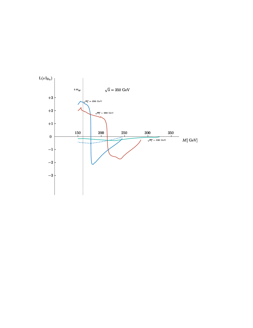
Figure 18: ${\mathrm{D}}_{0}\,$-function integrated over $u_{1}$ at $\sqrt{s}=350~{}\text{GeV}$ and for three values of $s_{1}$.

More boxes

Other examples involving box diagrams are ${}{{}{{{{{\mathrm{{{}{}{{g}}\mspace{-0.6mu}}}}}}}}}+{}{{}{{{{{\mathrm{{{}{}{{g}}\mspace{-0.6mu}}}}}}}}}({}{{}{{{{{\mathrm{{{}{}{{{}{{}{{{{{\mathrm{{{}{}{{e}}\mspace{-0.6mu}}}}}}}}}}^{+}}\mspace{-0.6mu}}}}}}}}}+{}{{}{{{{{\mathrm{{{}{}{{{}{{}{{{{{\mathrm{{{}{}{{e}}\mspace{-0.6mu}}}}}}}}}}^{-}}\mspace{-0.6mu}}}}}}}}})\to{}{{}{{{{{\mathrm{{{}{}{{{}{{}{{{{{\mathrm{{{}{}{{W}}\mspace{-0.6mu}}}}}}}}}}^{+}}\mspace{-0.6mu}}}}}}}}}+{}{{}{{{{{\mathrm{{{}{}{{{}{{}{{{{{\mathrm{{{}{}{{W}}\mspace{-0.6mu}}}}}}}}}}^{-}}\mspace{-0.6mu}}}}}}}}}+{}{{}{{{{{\mathrm{{{}{}{{H}}\mspace{-0.6mu}}}}}}}}}$, with an on-shell Higgs boson and, at least, one off-shell ${}{{}{{{{{\mathrm{{{}{}{{W}}\mspace{-0.6mu}}}}}}}}}$. Here ${}{{}{{{{{\mathrm{{{}{}{{g}}\mspace{-0.6mu}}}}}}}}}+{}{{}{{{{{\mathrm{{{}{}{{g}}\mspace{-0.6mu}}}}}}}}}\to{}{{}{{{{{\mathrm{{{}{}{{g}}\mspace{-0.6mu}}}}}}}}}$ or ${}{{}{{{{{\mathrm{{{}{}{{{}{{}{{{{{\mathrm{{{}{}{{e}}\mspace{-0.6mu}}}}}}}}}}^{+}}\mspace{-0.6mu}}}}}}}}}+{}{{}{{{{{\mathrm{{{}{}{{{}{{}{{{{{\mathrm{{{}{}{{e}}\mspace{-0.6mu}}}}}}}}}}^{-}}\mspace{-0.6mu}}}}}}}}}\to{}{{}{{{{{\mathrm{{{}{}{{Z}}\mspace{-0.6mu}}}}}}}}}/{}{{}{{{{{\mathrm{{{}{}{}\mspace{-0.6mu}}}}}}}}}$ with ${}{{}{{{{{\mathrm{{{}{}{{g}}\mspace{-0.6mu}}}}}}}}}({}{{}{{{{{\mathrm{{{}{}{{Z}}\mspace{-0.6mu}}}}}}}}}/{}{{}{{{{{\mathrm{{{}{}{}\mspace{-0.6mu}}}}}}}}})$ attached to a box where the other external lines are ${}{{}{{{{{\mathrm{{{}{}{{W}}\mspace{-0.6mu}}}}}}}}}{}{{}{{{{{\mathrm{{{}{}{{W}}\mspace{-0.6mu}}}}}}}}}$ and the Higgs boson (coupled to ${}{{}{{{{{\mathrm{{{}{}{{b}}\mspace{-0.6mu}}}}}}}}}$ internal lines).

5.1 Anomalous threshold and gauge invariance

Given the amplitude for a process supporting an anomalous threshold within the physical region we would like to split it into two components, i.e. ${\mathrm{A}}_{\mathrm{\scriptscriptstyle{AT}}}+{\mathrm{A}}_{{\mbox{\scriptsize reg}}}$. In order to have a meaningful result we must discuss gauge invariance. Consider an of-shell gluon producing a ${}{}{{}{{}{{{{{\mathrm{{{}{}{{\overline{{}{{}{{{{{\mathrm{{{}{}{{b}}\mspace{-0.6mu}}}}}}}}}}}_{{\mspace{1.0mu}}}^{\mspace{1.0mu}{{\raisebox{-1.65764pt}{{${{{\scriptstyle{{{{{\mathrm{{}}}}}}}}}}$}}}}}}\mspace{-0.6mu}}}}}}}}}}{}{{}{{{{{\mathrm{{{}{}{{b}}\mspace{-0.6mu}}}}}}}}}$ pair and an heavy Higgs, e.g. the one in the singlet extension of the SM; the full process will be ${}{{}{{{{{\mathrm{{{}{}{{g}}\mspace{-0.6mu}}}}}}}}}+{}{{}{{{{{\mathrm{{{}{}{{g}}\mspace{-0.6mu}}}}}}}}}\to{}{}{{}{{}{{{{{\mathrm{{{}{}{{\overline{{}{{}{{{{{\mathrm{{{}{}{{b}}\mspace{-0.6mu}}}}}}}}}}}_{{\mspace{1.0mu}}}^{\mspace{1.0mu}{{\raisebox{-1.65764pt}{{${{{\scriptstyle{{{{{\mathrm{{}}}}}}}}}}$}}}}}}\mspace{-0.6mu}}}}}}}}}}+{}{{}{{{{{\mathrm{{{}{}{{b}}\mspace{-0.6mu}}}}}}}}}+{}{{}{{{{{\mathrm{{{}{}{{H}}\mspace{-0.6mu}}}}}}}}}$. To discuss gauge invariance we work in the ${\mathrm{R}}_{\xi}\,$-gauge where propagators are

$${}{{}{{{{{\mathrm{{{}{}{{W}}\mspace{-0.6mu}}}}}}}}}\;\to\;\frac{1}{p^{2}+M^{2}_{{}{{}{{{{{\mathrm{{{}{}{{W}}\mspace{-0.6mu}}}}}}}}}}}\,\left(\delta_{\mu\nu}+\frac{p_{\mu}\,p_{\nu}}{M^{2}_{{}{{}{{{{{\mathrm{{{}{}{{W}}\mspace{-0.6mu}}}}}}}}}}}\right)-\frac{p_{\mu}\,p_{\nu}}{M^{2}_{{}{{}{{{{{\mathrm{{{}{}{{W}}\mspace{-0.6mu}}}}}}}}}}\,(p^{2}+\xi^{2}\,M^{2}_{{}{{}{{{{{\mathrm{{{}{}{{W}}\mspace{-0.6mu}}}}}}}}}})}\,,\quad\upphi\;\to\;\frac{1}{p^{2}+\xi^{2}\,M^{2}_{{}{{}{{{{{\mathrm{{{}{}{{W}}\mspace{-0.6mu}}}}}}}}}}}\,,$$ (65)

where is a Higgs-Kibble ghost. Consider the four diagrams, family a), shown in Figure 12: it is easy to show that the corresponding AT can be physical. Next we perform a “scalarization” of the amplitude which gives a collection of ${\mathrm{D}}_{0}\,$-functions, ${\mathrm{C}}_{0}\,$-functions and ${\mathrm{B}}_{0}\,$-functions.

• It is easy to see that the $D_{0}$ part of the amplitude is $\xi\,$-independent, i.e. ${\mathrm{D}}_{0}\,$-functions depending on $\xi^{2}\,M^{2}_{{}{{}{{{{{\mathrm{{{}{}{{W}}\mspace{-0.6mu}}}}}}}}}}$ cancel. Therefore we could define ${\mathrm{A}}_{\mathrm{\scriptscriptstyle{AT}}}$ in terms of scalar boxes, including the rest in ${\mathrm{A}}_{{\mbox{\scriptsize reg}}}$.

• Alternatively, we can search for ${\mathrm{S}}_{\mathrm{\scriptscriptstyle{AT}}}$, the minimal subset of diagrams which is $\xi\,$-independent, satisfies Ward-Slavnov-Taylor identities (if applicable) and supports a physical-region AT. The corresponding procedure can be visualized as follows: scalarization produces triangles which are contractions of the original box, i.e. are obtained by shrinking one line of the box to a point; therefore, we must add family b), i.e. all boxes that give the same set of contractions (see Figure 19), and family c), i.e. all ${}{{}{{{{{\mathrm{{{}{}{{b}}\mspace{-0.6mu}}}}}}}}}{-}{}{{}{{{{{\mathrm{{{}{}{{b}}\mspace{-0.6mu}}}}}}}}}{-}{}{{}{{{{{\mathrm{{{}{}{{H}}\mspace{-0.6mu}}}}}}}}}$ (pure) triangles with a gluon coupled to ${}{{}{{{{{\mathrm{{{}{}{{b}}\mspace{-0.6mu}}}}}}}}}$ current.

Figure 19: Family b) for ${}{{}{{{{{\mathrm{{{}{}{{g}}\mspace{-0.6mu}}}}}}}}}(Q)\to{}{{}{{{{{\mathrm{{{}{}{{b}}\mspace{-0.6mu}}}}}}}}}(q_{1})+{}{}{{}{{}{{{{{\mathrm{{{}{}{{\overline{{}{{}{{{{{\mathrm{{{}{}{{b}}\mspace{-0.6mu}}}}}}}}}}}_{{\mspace{1.0mu}}}^{\mspace{1.0mu}{{\raisebox{-1.65764pt}{{${{{\scriptstyle{{{{{\mathrm{{}}}}}}}}}}$}}}}}}\mspace{-0.6mu}}}}}}}}}}(q_{3})+{}{{}{{{{{\mathrm{{{}{}{{H}}\mspace{-0.6mu}}}}}}}}}(q_{2})$.

5.1.1 Renormalization

As has been said many times our goal is not to perform the full calculation, therefore renormalization has to be understood in the ${\overline{\mathrm{MS}}}$ scheme with the renormalization scale set at the highest scale in the process under consideration.

5.1.2 $\pi^{2}$ enhancement

A ${\mathrm{C}}_{0}\,$-function is given by the integral

$${\mathrm{I}}=\int_{0}^{1}dx_{1}\,\int_{0}^{x_{1}}dx_{2}\,\Bigl{[}\sum_{i,j=1,2}\,(x_{1}-X_{i})\,{\mathrm{H}}_{ij}\,(x_{j}-X_{j})+\Delta_{3}\Bigr{]}^{-1}\,\,.$$ (66)

In general, in the complex mass scheme $\Delta_{3},X_{1,2}\in\mathbb{C}$. There are configurations where $\mid\Delta_{3}\mid\ll 1$, although far from the AT, and where $\mid{\mathrm{H}}_{11}\mid\ll 1$ (or $\mid{\mathrm{H}}_{22}\mid\ll 1$) with $0<\mathop{\mathrm{Re}}\nolimits X_{2}<1$ (or $0<\mathop{\mathrm{Re}}\nolimits X_{1}<1$ but not both). The condition for ${\mathrm{H}}_{ii}$ is always satisfied when we have light external particles. Therefore, choosing the case $\mid{\mathrm{H}}_{22}\mid\ll 1$, we can write

$${\mathrm{I}} \approx \int_{0}^{1}dx_{1}\,\int_{0}^{x_{1}}dx_{2}\,\Bigl{[}{\mathrm{H}}_{11}\,(x_{1}-X_{1})^{2}+2\,{\mathrm{H}}_{12}\,(x_{1}-X_{1})\,(x_{2}-X_{2})\Bigr{]}^{-1}$$ (67)

$$= \frac{1}{2}\,{\mathrm{H}}^{-1}_{12}\,\Bigl{\{}\Bigl{[}\ln(2\,{\mathrm{H}}_{12}\,(X_{1}-X_{2})-\ln(-2\,{\mathrm{H}}_{12}\,X_{2})\Bigr{]}\,\ln(1-\frac{1}{X_{1}})+\quad\mbox{di-logarithms}\quad\Bigr{\}}\,\,.$$

With $\mathop{\mathrm{Re}}\nolimits X_{1}\in[0\,,\,1]$ and $\mid\mathop{\mathrm{Im}}\nolimits X_{1}\mid\ll 1$ but $\mathop{\mathrm{Im}}\nolimits X_{1}>0$, we obtain

$${\mathrm{I}}\approx\frac{i\,\pi}{2}\,{\mathrm{H}}^{-1}_{12}\,\mathop{\mathrm{Re}}\nolimits\,\Bigl{[}\ln(2\,{\mathrm{H}}_{12}\,(X_{1}-X_{2})-\ln(-2\,{\mathrm{H}}_{12}\,X_{2})\Bigr{]}+\quad\mbox{rest}\,\,.$$ (68)

This ${\mathrm{C}}_{0}\,$-function will be part of the one-loop corrections to a given LO amplitude. Since ${\mathrm{A}}_{\mathrm{\scriptscriptstyle{LO}}}$ is in general real this “$i\,\pi$” term will not interfere but the NLO amplitude squared will receive a “$\pi^{2}$” enhancement. As we will see in the following sections this is often the case, resulting in NNLO corrections (the NLO squared) which are much larger than the NLO ones. Clearly, only a complete calculation can decide the fate of these “$\pi^{2}$" terms. Note that this enhancement should not be confused with the “pinch”, the latter requiring both $X_{1}$ and $X_{2}$ to be inside $[0\,,\,1]$.

5.2 The process ${}{{}{{{{{\mathrm{{{}{}{{g}}\mspace{-0.6mu}}}}}}}}}+{}{{}{{{{{\mathrm{{{}{}{{g}}\mspace{-0.6mu}}}}}}}}}\to{}{}{{}{{}{{{{{\mathrm{{{}{}{{\overline{{}{{}{{{{{\mathrm{{{}{}{{b}}\mspace{-0.6mu}}}}}}}}}}}_{{\mspace{1.0mu}}}^{\mspace{1.0mu}{{\raisebox{-1.65764pt}{{${{{\scriptstyle{{{{{\mathrm{{}}}}}}}}}}$}}}}}}\mspace{-0.6mu}}}}}}}}}}+{}{{}{{{{{\mathrm{{{}{}{{b}}\mspace{-0.6mu}}}}}}}}}+{}{{}{{{{{\mathrm{{{}{}{{X}}\mspace{-0.6mu}}}}}}}}}$

The full process to be studied will be

$${}{{}{{{{{\mathrm{{{}{}{{g}}\mspace{-0.6mu}}}}}}}}}(p_{1})+{}{{}{{{{{\mathrm{{{}{}{{g}}\mspace{-0.6mu}}}}}}}}}(p_{2})\to{}{{}{{{{{\mathrm{{{}{}{{b}}\mspace{-0.6mu}}}}}}}}}(q_{1})+{}{{}{{{{{\mathrm{{{}{}{{X}}\mspace{-0.6mu}}}}}}}}}(q_{2})+{}{}{{}{{}{{{{{\mathrm{{{}{}{{\overline{{}{{}{{{{{\mathrm{{{}{}{{b}}\mspace{-0.6mu}}}}}}}}}}}_{{\mspace{1.0mu}}}^{\mspace{1.0mu}{{\raisebox{-1.65764pt}{{${{{\scriptstyle{{{{{\mathrm{{}}}}}}}}}}$}}}}}}\mspace{-0.6mu}}}}}}}}}}(q_{3})\,,$$ (69)

requiring the following set of invariants:

$$s=-P^{2}=-(p_{1}+p_{2})^{2}\,,\quad s_{1}=-(P-q_{1})^{2}\,,\quad u_{1}=-(P-q_{2})^{2}\,,\quad t_{0}=-(p_{1}-q_{1})^{2}\,,\quad t_{1}=-(p_{1}-q_{2})^{2}\,\,.$$ (70)

Here ${}{{}{{{{{\mathrm{{{}{}{{X}}\mspace{-0.6mu}}}}}}}}}$ is a scalar state of invariant mass ${\mathrm{M}}$. Therefore it can represent some heavy BSM Higgs boson, a pair of SM Higgs boson (${}{{}{{{{{\mathrm{{{}{}{{g}}\mspace{-0.6mu}}}}}}}}}{}{{}{{{{{\mathrm{{{}{}{{g}}\mspace{-0.6mu}}}}}}}}}\to{}{}{{}{{}{{{{{\mathrm{{{}{}{{\overline{{}{{}{{{{{\mathrm{{{}{}{{b}}\mspace{-0.6mu}}}}}}}}}}}_{{\mspace{1.0mu}}}^{\mspace{1.0mu}{{\raisebox{-1.65764pt}{{${{{\scriptstyle{{{{{\mathrm{{}}}}}}}}}}$}}}}}}\mspace{-0.6mu}}}}}}}}}}{}{{}{{{{{\mathrm{{{}{}{{b}}\mspace{-0.6mu}}}}}}}}}{}{{}{{{{{\mathrm{{{}{}{{H}}\mspace{-0.6mu}}}}}}}}}{}{{}{{{{{\mathrm{{{}{}{{H}}\mspace{-0.6mu}}}}}}}}}$), a pair of ${}{{}{{{{{\mathrm{{{}{}{{W}}\mspace{-0.6mu}}}}}}}}}$ bosons (${}{{}{{{{{\mathrm{{{}{}{{g}}\mspace{-0.6mu}}}}}}}}}{}{{}{{{{{\mathrm{{{}{}{{g}}\mspace{-0.6mu}}}}}}}}}\to{}{}{{}{{}{{{{{\mathrm{{{}{}{{\overline{{}{{}{{{{{\mathrm{{{}{}{{b}}\mspace{-0.6mu}}}}}}}}}}}_{{\mspace{1.0mu}}}^{\mspace{1.0mu}{{\raisebox{-1.65764pt}{{${{{\scriptstyle{{{{{\mathrm{{}}}}}}}}}}$}}}}}}\mspace{-0.6mu}}}}}}}}}}{}{{}{{{{{\mathrm{{{}{}{{b}}\mspace{-0.6mu}}}}}}}}}{}{{}{{{{{\mathrm{{{}{}{{{}{{}{{{{{\mathrm{{{}{}{{W}}\mspace{-0.6mu}}}}}}}}}}^{+}}\mspace{-0.6mu}}}}}}}}}{}{{}{{{{{\mathrm{{{}{}{{{}{{}{{{{{\mathrm{{{}{}{{W}}\mspace{-0.6mu}}}}}}}}}}^{-}}\mspace{-0.6mu}}}}}}}}}$).

For real masses we observe that the region of phase space containing ATs becomes smaller and smaller when $s$ increases and disappears for $\sqrt{s}$ approximately greater that $438.5~{}\text{GeV}$. This is not the case for Peierls zeros; we have analyzed those zeros which are inside the physical phase space and for which

$$0\;<\;\mathop{\mathrm{Re}}\nolimits\,X_{3}\;<\;\mathop{\mathrm{Re}}\nolimits\,X_{2}\;<\;\mathop{\mathrm{Re}}\nolimits\,X_{1}\;<\;1\,\,.$$ (71)

To give an example we consider $\sqrt{s}=865~{}\text{GeV}$ and $\sqrt{s_{1}}=516.21~{}\text{GeV}$. There are four solutions to $\Delta_{4}=0$ and one of them satisfies the requested conditions, corresponding to ${\mathrm{M}}=308.06~{}\text{GeV}$ and $\sqrt{u_{1}}=556.94~{}\text{GeV}$ with

$$X_{3}=0.186+i\,0.977\,10^{-3}\,,\quad X_{2}=0.250-i\,0.171\,10^{-2}\,,\quad X_{1}=0.625+i\,0.793\,10^{-3}\,\,.$$ (72)

The evaluation of loop integrals which are regular when the corresponding BST factor is zero requires an additional comment: when internal masses are real the solution has been described in Ref. [51]. For instance, consider the three-point function, characterized by a polynomial

$${\mathrm{V}}(x_{1}\,,\,x_{2})-i\,0=\Bigl{[}{\mathrm{V}}_{0}(x_{1}\,,\,x_{2})-i\,0\Bigr{]}+\left(\Delta_{3}-i\,0\right)\,\,.$$ (73)

In section 4.4.1. of Ref. [51] it is found that one can write

$${\mathrm{C}}_{0}=\frac{1}{\Delta_{3}}\,\Bigl{[}\int\,dS_{2}\,\ln\frac{{\mathrm{V}}}{{\mathrm{V}}_{0}}-\frac{1}{2}\,\sum_{i=0}^{2}\,(X_{i}-X_{i+1})\,\int\,dS_{1}\,\ln\frac{{\mathrm{V}}(\widehat{i\;i+1})}{{\mathrm{V}}_{0}(\widehat{i\;i+1})}\Bigr{]}\,\,.$$ (74)

When complex masses are introduced the imaginary part of ${\mathrm{V}}$ has always the same sign, but this is not the case for ${\mathrm{V}}_{0}$; furthermore, $\mathop{\mathrm{Im}}\nolimits{\mathrm{V}}$ and $\mathop{\mathrm{Im}}\nolimits{\mathrm{V}}_{0}$ have, in general, different signs so that one cannot reconstruct terms like $\ln({\mathrm{V}}/{\mathrm{V}}_{0})$ as done in Eq.(74). Therefore, we will write

$${\mathrm{V}}(x_{1}\,,\,x_{2}\,;\,\{{\mathrm{I}}\})={\mathrm{V}}_{0}(x_{1}\,,\,x_{2}\,;\,\{{\mathrm{I}}\})+\Delta_{3}(\{{\mathrm{I}}\})\,,$$ (75)

where $\{{\mathrm{I}}\}$ is the set of invariants describing the process. When

$$\Delta_{3}(\{\overline{{\mathrm{I}}}\})=0\,,$$ (76)

we will subtract, with a double BST algorithm, ${\mathrm{V}}_{0}(x_{1}\,,\,x_{2}\,;\,\{\overline{{\mathrm{I}}}\})$ taking care of reconstructing $\ln({\mathrm{V}}/{\mathrm{V}}_{0})$ only when $\mid\Delta_{3}\mid$ is small enough and the imaginary parts of numerator and denominator have the same sign. Summarizing: let $\overline{X}_{i}=X_{i}(\{\overline{{\mathrm{I}}}\})$, we will use

$$\Bigl{[}1+\frac{1}{2\,(\mu+1)}\,(x-X)^{\mathrm{t}}\,\partial_{x}\Bigr{]}\,{\mathrm{V}}^{\mu+1}(x_{1}\,,\,x_{2}\,;\,\{{\mathrm{I}}\}) = \Delta_{3}(\{{\mathrm{I}}\})\,{\mathrm{V}}^{\mu}(x_{1}\,,\,x_{2}\,;\,\{{\mathrm{I}}\})\,,$$

$$\Bigl{[}1+\frac{1}{2\,(\mu+1)}\,(x-{\overline{X}})^{\mathrm{t}}\,\partial_{x}\Bigr{]}\,{\mathrm{V}}^{\mu+1}_{0}(x_{1}\,,\,x_{2}\,;\,\{{\overline{{\mathrm{I}}}}\}) = 0\,,$$ (77)

subtract the two equations and integrate by parts.

For ${}{{}{{{{{\mathrm{{{}{}{{g}}\mspace{-0.6mu}}}}}}}}}+{}{{}{{{{{\mathrm{{{}{}{{g}}\mspace{-0.6mu}}}}}}}}}\to{}{}{{}{{}{{{{{\mathrm{{{}{}{{\overline{{}{{}{{{{{\mathrm{{{}{}{{b}}\mspace{-0.6mu}}}}}}}}}}}_{{\mspace{1.0mu}}}^{\mspace{1.0mu}{{\raisebox{-1.65764pt}{{${{{\scriptstyle{{{{{\mathrm{{}}}}}}}}}}$}}}}}}\mspace{-0.6mu}}}}}}}}}}+{}{{}{{{{{\mathrm{{{}{}{{b}}\mspace{-0.6mu}}}}}}}}}+PX$ where ${}{{}{{{{{\mathrm{{{}{}{{X}}\mspace{-0.6mu}}}}}}}}}$ is an off-shell SM Higgs boson or an on-shell BSM Higgs boson the first three invariants in Eq.(70) are

$$s_{1-}\leq s_{1}\leq s_{1+}\,,\dots\,,t_{0-}\leq t_{0}\leq t_{0+}\,,$$ (78)

and we introduce new, scaled variables,

$$s_{1}=(s_{1+}-s_{1-})\,y_{1}+s_{1-}\,,\dots\,,t_{0}=(t_{0+}-t_{0-})\,y_{3}+t_{0-}\,\,.$$ (79)

For the last invariant in Eq.(70) we use $\lambda_{1}=\lambda(s\,,\,s_{1}\,,\,m^{2}_{{}{{}{{{{{\mathrm{{{}{}{{b}}\mspace{-0.6mu}}}}}}}}}})$ and $\lambda_{3}=\lambda(s\,,\,u_{1}\,,\,{\mathrm{M}}^{2})$ and define

$$\xi=(s-s_{1}+2\,t_{0}-m^{2}_{{}{{}{{{{{\mathrm{{{}{}{{b}}\mspace{-0.6mu}}}}}}}}}})\,\lambda^{-1/2}_{1}\,,\qquad\eta=\Bigl{[}2\,s\,(s_{1}+{\mathrm{M}}^{2})-(s+s_{1})\,(s-u_{1}+{\mathrm{M}}^{2})-m^{2}_{{}{{}{{{{{\mathrm{{{}{}{{b}}\mspace{-0.6mu}}}}}}}}}}\,(s+u_{1}-{\mathrm{M}}^{2})\Bigr{]}\,(\lambda_{1}\,\lambda_{3})^{-1/2}\,\,.$$ (80)

Next we introduce

$${\mathrm{z}}=\pi\,(y_{4}-\frac{1}{2})\,,\qquad y_{4}\in[0\,,\,1]\,,$$ (81)

and obtain

$$t_{1}=\frac{1}{2}\,\Bigl{\{}\Bigl{[}(\xi\,\eta)^{1/2}\,\sin({\mathrm{z}})+\xi\,\eta\Bigr{]}\,\lambda^{1/2}_{3}-s+u_{1}+{\mathrm{M}}^{2}\Bigr{\}}\,\,.$$ (82)

The object of interest (fully differential) is

$$\frac{d^{4}\,\sigma}{dy_{1}\,\dots\,dy_{4}}=\frac{1}{32\,\pi^{3}}\,\frac{s_{1+}-s_{1-}}{512\,s_{1}\,s^{2}}\,(\lambda_{1}\,\lambda_{2})^{1/2}\,\sum_{s,c}\,\mid{\mathrm{A}}\mid^{2}\,,$$ (83)

where $\lambda_{1}=\lambda(s\,,\,s_{1}\,,\,m^{2}_{{}{{}{{{{{\mathrm{{{}{}{{b}}\mspace{-0.6mu}}}}}}}}}})$ and $\lambda_{2}=\lambda(s_{1}\,,\,{\mathrm{M}}^{2}\,,\,m^{2}_{{}{{}{{{{{\mathrm{{{}{}{{b}}\mspace{-0.6mu}}}}}}}}}})$. The sum is over spin and color, ${\mathrm{A}}$ is the amplitude. Finally,

$$s_{1-}=({\mathrm{M}}+m_{{}{{}{{{{{\mathrm{{{}{}{{b}}\mspace{-0.6mu}}}}}}}}}})^{2}\,,\qquad s_{1+}=(\sqrt{s}-m_{{}{{}{{{{{\mathrm{{{}{}{{b}}\mspace{-0.6mu}}}}}}}}}})^{2}\,\,.$$ (84)

Both LO and interference with one-loop corrections are proportional to $m^{2}_{{}{{}{{{{{\mathrm{{{}{}{{b}}\mspace{-0.6mu}}}}}}}}}}$ while one-loop squared survives the limit $m_{{}{{}{{{{{\mathrm{{{}{}{{b}}\mspace{-0.6mu}}}}}}}}}}\to 0$. Loop effects are suppressed by a factor $g^{2}/(16\,\pi^{2})=0.0027$ which, however is of the same order of magnitude of the Yukawa suppression $m^{2}_{{}{{}{{{{{\mathrm{{{}{}{{b}}\mspace{-0.6mu}}}}}}}}}}/M^{2}_{{}{{}{{{{{\mathrm{{{}{}{{W}}\mspace{-0.6mu}}}}}}}}}}\approx 0.0021$. Therefore, we expect one-loop squared to be of the same order of the interference.

We selected $\sqrt{s}=865~{}\text{GeV}$ and ${\mathrm{M}}=308.06~{}\text{GeV}$. In the four-dimensional $y\,$-space there are trajectories feeling the presence of the Peierls zero, for instance, with $y_{3}=y_{4}=0.3$ and $y_{2}=0.6$ we have (NNLO is up to one-loop squared)

$$\begin{array}[]{lccc}{}&\;\;y_{1}=0.25&\;\;y_{1}=0.2626&\;\;y_{1}=0.27\\ \delta^{\mathrm{\scriptscriptstyle{AT}}}_{\mathrm{\scriptscriptstyle{NLO}}}[\%]&\;\;8.14&\;\;3.66&\;\;8.41\\ \delta^{\mathrm{\scriptscriptstyle{AT}}}_{\mathrm{\scriptscriptstyle{NNLO}}}[\%]&\;\;87.03&\;\;370.25&\;\;84.32\end{array}$$

It is worth noting the very large NNLO effect, induced by the “$\pi^{2}$’ terms which originates from triangles, as explained in subsubsection 5.1.2. For comparison we give $\delta^{\mathrm{\scriptscriptstyle{AT}}}_{\mathrm{\scriptscriptstyle{NNLO}}}$ for different values of $\sqrt{s}$ with ${\mathrm{M}}$ fixed and $y_{1}=0.2626$, $y_{2}=0.6$, $y_{3}=y_{4}=0.3$:

$$\begin{array}[]{lccc}\sqrt{s}[~{}\text{GeV}]&\;\;350&\;\;550&\;\;865\\ \delta^{\mathrm{\scriptscriptstyle{AT}}}_{\mathrm{\scriptscriptstyle{NNLO}}}&\;\;-0.68&\;\;10.56&\;\;370.25\end{array}$$

showing the combined effect of the Peierls zero and the “$\pi^{2}$" terms. Unfortunately, when more ($y$) integrations are performed the effect becomes less and less visible; for instance in the two-dimensional distribution, $y_{1}{-}y_{2}$, trajectories are almost flat in the $y_{1}(y_{2})$ direction. This seems to be a general result: for processes requiring more and more invariants the fully inclusive observables become less and less sensitive to ATs.

5.3 The process ${}{{}{{{{{\mathrm{{{}{}{{g}}\mspace{-0.6mu}}}}}}}}}+{}{{}{{{{{\mathrm{{{}{}{{g}}\mspace{-0.6mu}}}}}}}}}\to{}{}{{}{{}{{{{{\mathrm{{{}{}{{\overline{{}{{}{{{{{\mathrm{{{}{}{{b}}\mspace{-0.6mu}}}}}}}}}}}_{{\mspace{1.0mu}}}^{\mspace{1.0mu}{{\raisebox{-1.65764pt}{{${{{\scriptstyle{{{{{\mathrm{{}}}}}}}}}}$}}}}}}\mspace{-0.6mu}}}}}}}}}}+{}{{}{{{{{\mathrm{{{}{}{{b}}\mspace{-0.6mu}}}}}}}}}+{}{{}{{{{{\mathrm{{{}{}{{H}}\mspace{-0.6mu}}}}}}}}}+{}{{}{{{{{\mathrm{{{}{}{{H}}\mspace{-0.6mu}}}}}}}}}$

There are several classes of diagrams contributing to the process. In Figure 20 diagrams of class a) have an AT inside the physical region; diagrams of class b) do not have an AT but are needed for gauge invariance when we move beyond the ${\mathrm{D}}_{0}\,$-approximation. Diagrams in Figure 21 include pentagons which do not have a leading singularity in the physical region but show a subleading one (box driven) obtained by shrinking one line of the pentagon to a point.

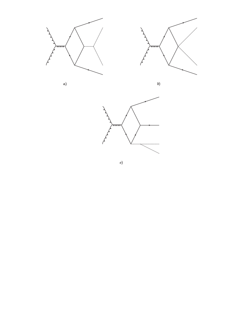
Figure 20: Diagrams contributing to ${}{{}{{{{{\mathrm{{{}{}{{g}}\mspace{-0.6mu}}}}}}}}}+{}{{}{{{{{\mathrm{{{}{}{{g}}\mspace{-0.6mu}}}}}}}}}\to{}{}{{}{{}{{{{{\mathrm{{{}{}{{\overline{{}{{}{{{{{\mathrm{{{}{}{{b}}\mspace{-0.6mu}}}}}}}}}}}_{{\mspace{1.0mu}}}^{\mspace{1.0mu}{{\raisebox{-1.65764pt}{{${{{\scriptstyle{{{{{\mathrm{{}}}}}}}}}}$}}}}}}\mspace{-0.6mu}}}}}}}}}}+{}{{}{{{{{\mathrm{{{}{}{{b}}\mspace{-0.6mu}}}}}}}}}+{}{{}{{{{{\mathrm{{{}{}{{H}}\mspace{-0.6mu}}}}}}}}}+{}{{}{{{{{\mathrm{{{}{}{{H}}\mspace{-0.6mu}}}}}}}}}$.

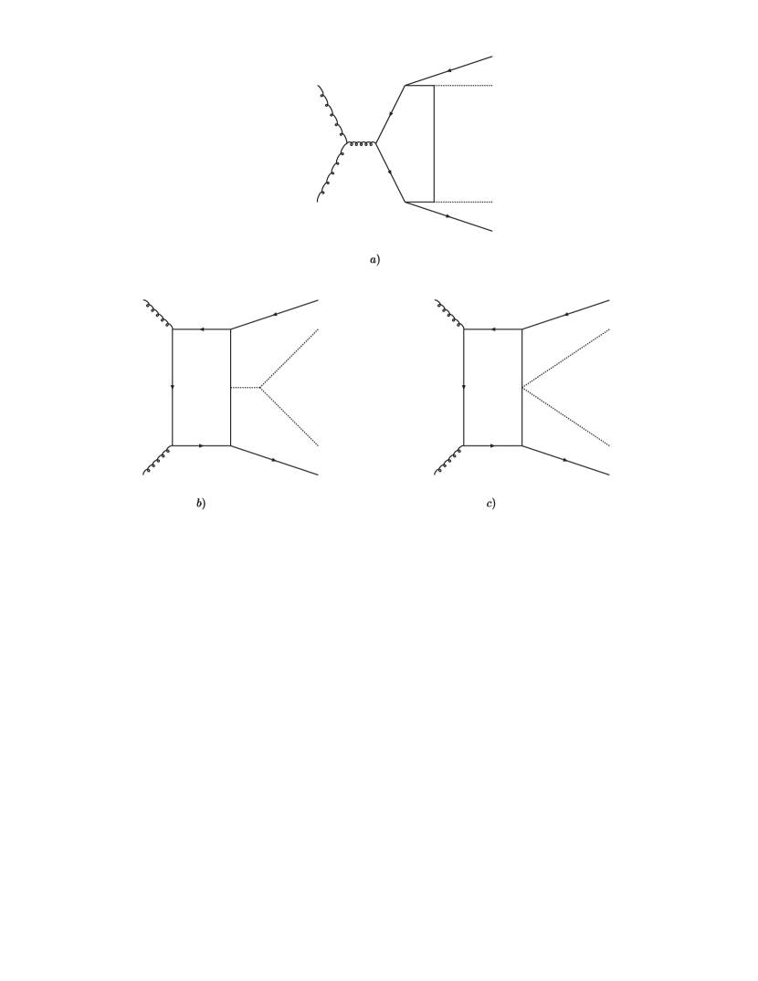
Figure 21: Diagrams contributing to ${}{{}{{{{{\mathrm{{{}{}{{g}}\mspace{-0.6mu}}}}}}}}}+{}{{}{{{{{\mathrm{{{}{}{{g}}\mspace{-0.6mu}}}}}}}}}\to{}{}{{}{{}{{{{{\mathrm{{{}{}{{\overline{{}{{}{{{{{\mathrm{{{}{}{{b}}\mspace{-0.6mu}}}}}}}}}}}_{{\mspace{1.0mu}}}^{\mspace{1.0mu}{{\raisebox{-1.65764pt}{{${{{\scriptstyle{{{{{\mathrm{{}}}}}}}}}}$}}}}}}\mspace{-0.6mu}}}}}}}}}}+{}{{}{{{{{\mathrm{{{}{}{{b}}\mspace{-0.6mu}}}}}}}}}+{}{{}{{{{{\mathrm{{{}{}{{H}}\mspace{-0.6mu}}}}}}}}}+{}{{}{{{{{\mathrm{{{}{}{{H}}\mspace{-0.6mu}}}}}}}}}$.

6 Pentagons

As shown in Ref. [52] there is no discontinuity associated with the LLS of the pentagon. This is why Ref. [65] refers to the singularity as a pole, i.e. ${\mathrm{E}}_{0}\sim 1/\Delta_{5}$, as shown in Ref. [51].

Consider the diagram of Figure 22 with $Q^{2}=-s$, $q^{2}_{i}=-{\mathrm{M}}^{2}_{i}$. The corresponding process is described in terms of the following set of invariant:

$$s_{1}=-(Q-q_{1})^{2}\,,\quad s_{2}=-(Q-q_{1}-q_{2})^{2}\,,\quad u_{1}=-(Q-q_{2})^{2}\,,\quad u_{2}=-(Q-q_{3})^{2}\,,\quad t_{2}=-(Q-q_{2}-q_{3})^{2}\,\,.$$ (85)

Their limits, the physical region, are:

$$({\mathrm{M}}_{2}+{\mathrm{M}}_{3}+{\mathrm{M}}_{4})^{2}\leq s_{1}\leq(\sqrt{s}-{\mathrm{M}}_{1})^{2}\,,\qquad({\mathrm{M}}_{3}+{\mathrm{M}}_{4})^{2}\leq s_{2}\leq(\sqrt{s_{1}}-{\mathrm{M}}_{2})^{2}\,,$$ (86)

and $u_{1-}\leq u_{1}\leq u_{1+}$ etc. where the limits can be written as $u_{1\pm}=u_{10}\pm du_{1}$ etc. with the following explicit expressions (see Ref. [91] for details),

$$u_{10}=s+{\mathrm{M}}^{2}_{2}-\frac{1}{2\,s_{1}}\,(s_{1}-s_{2}+{\mathrm{M}}^{2}_{2})\,(s+s_{1}-{\mathrm{M}}^{2}_{1})\,,\quad\Delta u_{1}=\frac{1}{2\,s_{1}}\,\lambda_{1}\,\lambda_{2}\,,$$

$$u_{20}=s+{\mathrm{M}}^{2}_{3}-\frac{1}{2\,s_{2}}\,(s_{2}+{\mathrm{M}}^{2}_{3}-{\mathrm{M}}^{2}_{4})\,(s+s_{2}-s^{\prime}_{2})\,,\quad\Delta u_{2}=\frac{1}{2\,s_{2}}\,\lambda_{3}\,\lambda_{4}\,,$$

$$t_{20}=u_{1}+{\mathrm{M}}^{2}_{3}-\frac{1}{2\,s}\,(s-u_{2}+{\mathrm{M}}^{2}_{3})\,(s+u_{1}-{\mathrm{M}}^{2}_{2})-\frac{1}{2}\,\frac{\xi_{2}\eta_{2}}{s}\,\lambda_{5}\,\lambda_{6}\,,\quad dt_{2}=\frac{1}{2\,s}\,(1-\xi^{2}_{2})^{1/2}\,(1-\eta^{2}_{2})^{1/2}\,\lambda_{5}\,\lambda_{6}\,\,.$$ (87)

Variables $\lambda_{1},\,\dots\,,\lambda_{6}$ are defined in terms of the following Källen lambda functions:

$$\lambda_{1} = \lambda^{1/2}(s\,,\,s_{1}\,,\,{\mathrm{M}}^{2}_{1})\,,\quad\lambda_{2}=\lambda^{1/2}(s_{1}\,,\,s_{2}\,,\,{\mathrm{M}}^{2}_{2})\,,\quad\lambda_{3}=\lambda^{1/2}(s\,,\,s_{2}\,,\,s^{\prime}_{2})\,,$$

$$\lambda_{4} = \lambda^{1}{2}(s_{2}\,,\,{\mathrm{M}}^{2}_{3}\,,\,{\mathrm{M}}^{2}_{4})\,,\quad\lambda_{5}=\lambda^{1/2}(s\,,\,u_{1}\,,\,{\mathrm{M}}^{2}_{2})\,,\quad\lambda_{6}=\lambda^{1/2}(s\,,\,u_{2}\,,\,{\mathrm{M}}^{2}_{3})\,\,.$$ (88)

We have also introduced additional variables

$$s^{\prime}_{2}=s-s_{1}+s_{2}-u_{1}+{\mathrm{M}}^{2}_{1}+{\mathrm{M}}^{2}_{2}\,,\qquad t^{\prime}_{1}={\mathrm{M}}^{2}_{2}\,\,.$$ (89)

The variables $\xi_{2}$ and $\eta_{2}$ can be found in Ref. [91] with full details on the calculation of the phase space.

The example to be discussed is as follows:

$${\mathrm{M}}_{1}=m_{{}{{}{{{{{\mathrm{{{}{}{{b}}\mspace{-0.6mu}}}}}}}}}}\,,\quad{\mathrm{M}}_{3}=0\,,\quad{\mathrm{M}}_{2}={\mathrm{M}}\,,\quad{\mathrm{M}}_{4}=m_{{}{{}{{{{{\mathrm{{{}{}{{b}}\mspace{-0.6mu}}}}}}}}}}\,,$$

$$m_{1}=m_{{}{{}{{{{{\mathrm{{{}{}{{t}}\mspace{-0.6mu}}}}}}}}}}\,,\quad m_{2}=M_{{}{{}{{{{{\mathrm{{{}{}{{W}}\mspace{-0.6mu}}}}}}}}}}\,,\quad m_{3}=0\,,\quad m_{4}=M_{{}{{}{{{{{\mathrm{{{}{}{{W}}\mspace{-0.6mu}}}}}}}}}}\,,\quad m_{t}=m_{{}{{}{{{{{\mathrm{{{}{}{{t}}\mspace{-0.6mu}}}}}}}}}}\,,$$ (90)

where $q_{3}$ is an electron and we have neglected the mass while line $3$ is a neutrino. In the limit of zero widths the equation $\Delta_{5}=0$ is quadratic in $t_{2}$; here $q_{2}$ is the momentum of a pair, electron-photon, so that what we are considering is ${}{{}{{{{{\mathrm{{{}{}{{g}}\mspace{-0.6mu}}}}}}}}}{}{{}{{{{{\mathrm{{{}{}{{g}}\mspace{-0.6mu}}}}}}}}}\to{}{{}{{{{{\mathrm{{{}{}{{g}}\mspace{-0.6mu}}}}}}}}}\to{}{}{{}{{}{{{{{\mathrm{{{}{}{{\overline{{}{{}{{{{{\mathrm{{{}{}{{b}}\mspace{-0.6mu}}}}}}}}}}}_{{\mspace{1.0mu}}}^{\mspace{1.0mu}{{\raisebox{-1.65764pt}{{${{{\scriptstyle{{{{{\mathrm{{}}}}}}}}}}$}}}}}}\mspace{-0.6mu}}}}}}}}}}{}{{}{{{{{\mathrm{{{}{}{{b}}\mspace{-0.6mu}}}}}}}}}{}{{}{{{{{\mathrm{{{}{}{{{}{{}{{{{{\mathrm{{{}{}{{e}}\mspace{-0.6mu}}}}}}}}}}^{-}}\mspace{-0.6mu}}}}}}}}}{}{{}{{{{{\mathrm{{{}{}{{{}{{}{{{{{\mathrm{{{}{}{{e}}\mspace{-0.6mu}}}}}}}}}}^{+}}\mspace{-0.6mu}}}}}}}}}{}{{}{{{{{\mathrm{{{}{}{}\mspace{-0.6mu}}}}}}}}}$. An example of physical-region ATs is given in the following table.

$$\begin{array}[]{rrrrrr}\mbox{fixed}&&&&&\mbox{solution}\\ \hline\cr{\mathrm{M}}_{2}[~{}\text{GeV}]&\sqrt{s_{1}}[~{}\text{GeV}]&\sqrt{s_{2}}[~{}\text{GeV}]&\sqrt{u_{1}}[~{}\text{GeV}]&\sqrt{u_{2}}[~{}\text{GeV}]&\sqrt{t_{2}}[~{}\text{GeV}]\\ \hline\cr 97.40&260.47&139.17&201.03&275.84&122.53\\ "&"&"&203.55&260.91&89.06\\ "&"&"&"&265.74&103.56\\ "&"&"&"&270.56&117.37\\ "&"&"&"&275.39&130.91\\ "&"&147.14&213.31&266.39&121.68\\ "&"&"&"&271.07&138.30\\ "&"&"&215.30&255.98&98.96\\ "&"&"&"&260.89&113.19\\ \hline\cr\end{array}$$

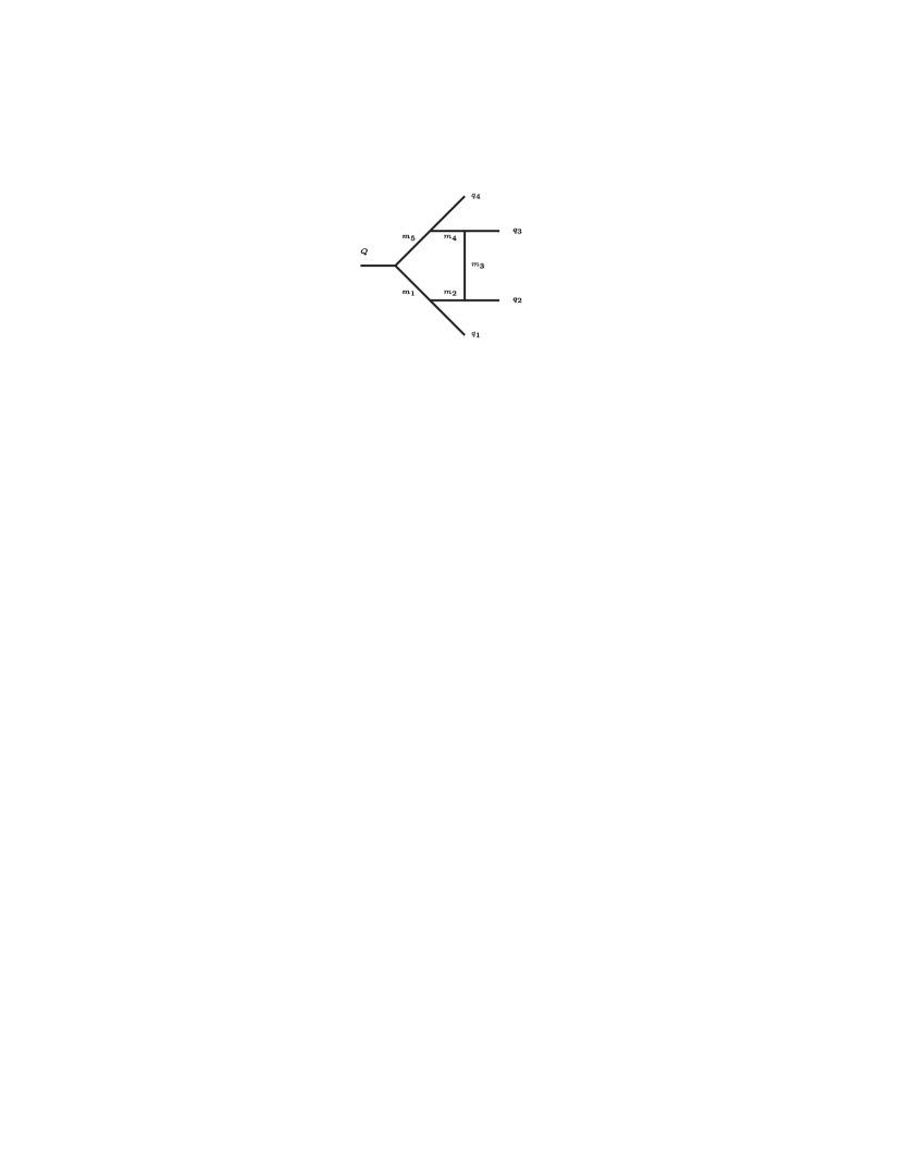
Figure 22: Pentagon diagram: the general case with arbitrary internal and external masses.

The same line of arguments applies to ${}{{}{{{{{\mathrm{{{}{}{{g}}\mspace{-0.6mu}}}}}}}}}{}{{}{{{{{\mathrm{{{}{}{{g}}\mspace{-0.6mu}}}}}}}}}\to{}{}{{}{{}{{{{{\mathrm{{{}{}{{\overline{{}{{}{{{{{\mathrm{{{}{}{{b}}\mspace{-0.6mu}}}}}}}}}}}_{{\mspace{1.0mu}}}^{\mspace{1.0mu}{{\raisebox{-1.65764pt}{{${{{\scriptstyle{{{{{\mathrm{{}}}}}}}}}}$}}}}}}\mspace{-0.6mu}}}}}}}}}}{}{{}{{{{{\mathrm{{{}{}{{b}}\mspace{-0.6mu}}}}}}}}}{}{}{{}{{}{{{{{\mathrm{{{}{}{{\overline{{}{{}{{{{{\mathrm{{{}{}{{u}}\mspace{-0.6mu}}}}}}}}}}}_{{\mspace{1.0mu}}}^{\mspace{1.0mu}{{\raisebox{-1.65764pt}{{${{{\scriptstyle{{{{{\mathrm{{}}}}}}}}}}$}}}}}}\mspace{-0.6mu}}}}}}}}}}{}{{}{{{{{\mathrm{{{}{}{{u}}\mspace{-0.6mu}}}}}}}}}{}{{}{{{{{\mathrm{{{}{}{{g}}\mspace{-0.6mu}}}}}}}}}$ or ${}{{}{{{{{\mathrm{{{}{}{{g}}\mspace{-0.6mu}}}}}}}}}{}{{}{{{{{\mathrm{{{}{}{{g}}\mspace{-0.6mu}}}}}}}}}\to{}{}{{}{{}{{{{{\mathrm{{{}{}{{\overline{{}{{}{{{{{\mathrm{{{}{}{{b}}\mspace{-0.6mu}}}}}}}}}}}_{{\mspace{1.0mu}}}^{\mspace{1.0mu}{{\raisebox{-1.65764pt}{{${{{\scriptstyle{{{{{\mathrm{{}}}}}}}}}}$}}}}}}\mspace{-0.6mu}}}}}}}}}}{}{{}{{{{{\mathrm{{{}{}{{b}}\mspace{-0.6mu}}}}}}}}}{}{}{{}{{}{{{{{\mathrm{{{}{}{{\overline{{}{{}{{{{{\mathrm{{{}{}{{d}}\mspace{-0.6mu}}}}}}}}}}}_{{\mspace{1.0mu}}}^{\mspace{1.0mu}{{\raisebox{-1.65764pt}{{${{{\scriptstyle{{{{{\mathrm{{}}}}}}}}}}$}}}}}}\mspace{-0.6mu}}}}}}}}}}{}{{}{{{{{\mathrm{{{}{}{{d}}\mspace{-0.6mu}}}}}}}}}{}{{}{{{{{\mathrm{{{}{}{{g}}\mspace{-0.6mu}}}}}}}}}$, with ${}{{}{{{{{\mathrm{{{}{}{{u}}\mspace{-0.6mu}}}}}}}}}\not={}{{}{{{{{\mathrm{{{}{}{{t}}\mspace{-0.6mu}}}}}}}}}$.

An interesting question is the following: consider a particle of invariant mass $\sqrt{s}$ “decaying” into a four-body final state; $\Delta_{5}$ is a quartic polynomial in $s$ and we look for complex solutions in the variable $s$ to the equation $\Delta_{5}=0$ with $0<\mathop{\mathrm{Re}}\nolimits X_{4}<\,\dots\,\mathop{\mathrm{Re}}\nolimits X_{1}<1$. Since the AT for a pentagon is a pole this is exactly the situation where the AT could be misinterpreted as the peak due to an unstable particle.

Deciding whether it is a resonance would require establishing that the “pole” is on the second (unphysical) sheet. In this case one of the external ‘masses”, i.e. $s$, is complex and $\ln^{-}({\mathrm{z}})\not=\ln({\mathrm{z}})$ etc. This fact requires a more complicated structure of the analytic continuation of the original integral including contour deformation, see section 6.6 of Ref. [82], which is beyond the scope of this work. Furthermore, the real analytic approach has the merit of working with quantities having a direct physical meaning and direct physical intuition is certainly of great help. The vertex function with three complex external masses has been discussed in Ref. [94].

7 Hexagons

For six point functions the leading Landau singularity is a sum of products of the Landau singularities for the reduced pentagon diagrams [52].

For $n\geq 6$ all the singularities of the one-loop $n\,$-point functions coincide with the singularities of the reduced, down to and including the pentagon, diagrams obtained from the main diagram [95, 96]. This result follows from the well-known property of vanishing of Gram determinants if any of its principal minors vanish. A plausible conclusion: at one loop a simple pole is the strongest possible singularity.

8 Two loop diagrams

So far we have discussed the leading Landau singularity for one-loop diagrams. In view of the impact of QCD corrections we would like to understand the behavior of two loop diagrams; this is, by far, more complicated than the one loop analysis, especially because we have no simple expression for the BST factor. Therefore, we have to resort to the set of Landau equations, written in momentum space. The full analysis for two loop triangles has been given in Ref. [97] and we will use the relevant results. For a diagram with $l$ loops and $n$ propagators we have $4\,l+n+1$ conditions on $4\,l+n$ variables; this means that a solution may exist only for specific values of external momenta. Consider the vertex of Figure 23, the Landau equation for this topology are as follows:

$$\begin{array}[]{lll}\alpha_{1}\,(q^{2}_{1}+m^{2}_{1})=0\,,&\qquad\alpha_{2}\,((q_{1}+P)^{2}+m^{2}_{2})=0\,,&\qquad\alpha_{3}\,((q_{1}-q_{2})^{2}+m^{2}_{3})=0\,,\\ \alpha_{4}\,(q_{2}^{2}+m^{2}_{4})=0\,,&\qquad\alpha_{5}\,((q_{2}+p_{1})^{2}+m^{2}_{5})=0\,,&\qquad\alpha_{6}\,((q_{2}+P)^{2}+m^{2}_{6})=0\,,\end{array}$$

and also

$$\alpha_{1}q_{1\mu}+\alpha_{2}(q_{1}+P)_{\mu}+\alpha_{3}(q_{1}-q_{2})_{\mu} = 0\,,$$

$$-\alpha_{3}(q_{1}-q_{2})_{\mu}+\alpha_{4}\,q_{2\mu}+\alpha_{5}\,(q_{2}+p_{1})_{\mu}+\alpha_{6}\,(q_{2}+P)_{\mu} = 0\,,$$ (91)

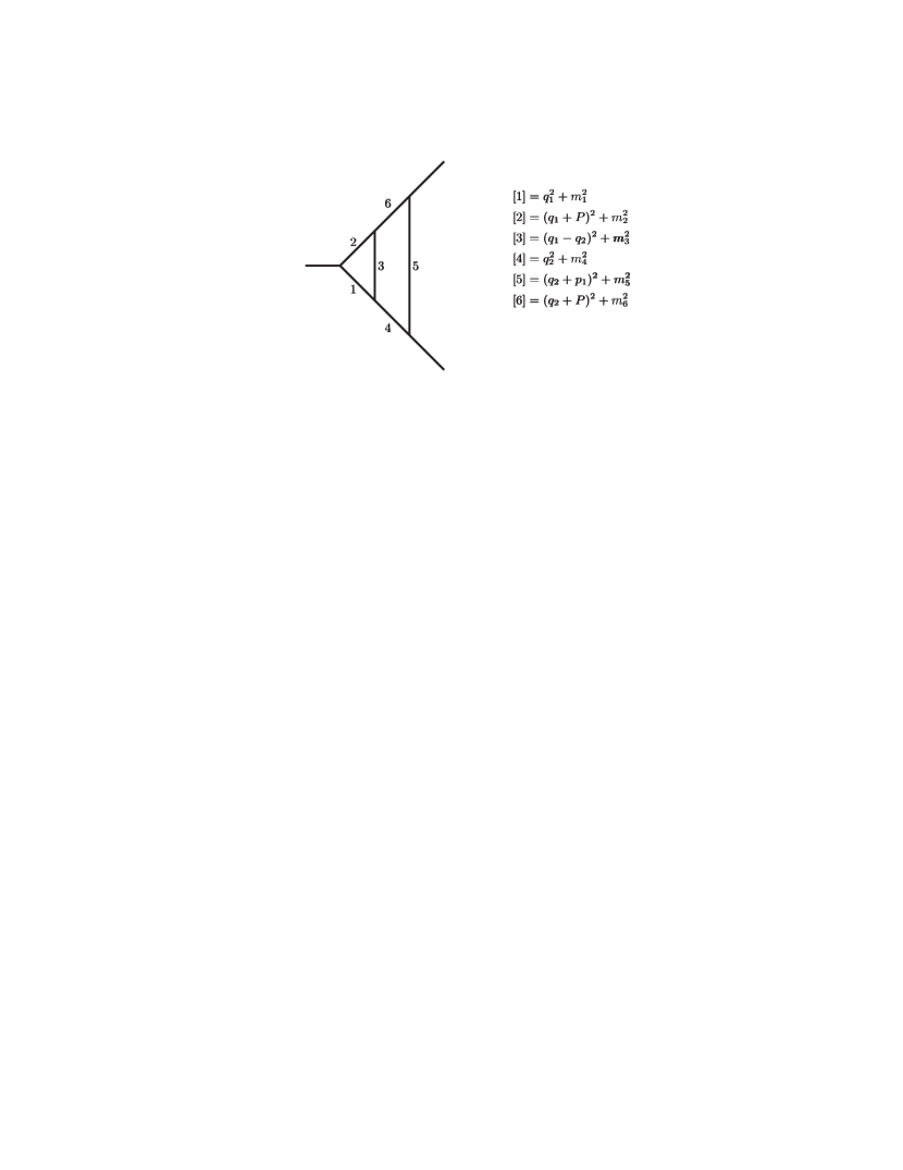
Figure 23: Two loop diagram. With $[i]$ we denote the inverse propagator for line $i$.

The leading Landau singularity occurs for $\alpha_{i}\neq 0,\forall i$. We multiply the two equations Eq.(91) by $q_{1\mu}$, $q_{2\mu}$, $p_{1\mu}$ and $P_{\mu}$, respectively. This gives an homogeneous system of eight equations. If all $\alpha_{i}$ are different from zero we may use

$$\begin{array}[]{lll}q^{2}_{1}=-m^{2}_{1}&\qquad q^{2}_{2}=-m^{2}_{4}\,,&\qquad{q_{1}}\cdot{q_{2}}=\frac{1}{2}\,(m^{2}_{3}-m^{2}_{1}-m^{2}_{4})\,,\\ {q_{1}}\cdot{P}=-\,\frac{1}{2}\,(P^{2}-m^{2}_{1}+m^{2}_{2})\,,&\qquad{q_{2}}\cdot{p_{1}}=-\,\frac{1}{2}\,(p_{1}^{2}-m^{2}_{4}+m^{2}_{5})\,,&\qquad{q_{2}}\cdot{P}=-\,\frac{1}{2}\,(P^{2}-m^{2}_{4}+m^{2}_{6})\,\,.\end{array}$$

Compatibility requires a set of relations among $P^{2},p^{2}_{1,2}$ and internal masses. If we select $m_{3}=0$ (gluon, photon), $m_{5}=m_{{}{{}{{{{{\mathrm{{{}{}{{b}}\mspace{-0.6mu}}}}}}}}}}$ and the remaining masses equal to $m_{{}{{}{{{{{\mathrm{{{}{}{{t}}\mspace{-0.6mu}}}}}}}}}}$ then a non trivial solution ($\alpha_{i}\neq 0,\forall i$) occurs iff

$$s=-P^{2}=4\,m^{2}_{{}{{}{{{{{\mathrm{{{}{}{{t}}\mspace{-0.6mu}}}}}}}}}}\,,\quad{\mathrm{M}}^{2}_{1}=-p^{2}_{1}=(m_{{}{{}{{{{{\mathrm{{{}{}{{t}}\mspace{-0.6mu}}}}}}}}}}\pm m_{{}{{}{{{{{\mathrm{{{}{}{{b}}\mspace{-0.6mu}}}}}}}}}})^{2}\,,\quad{\mathrm{M}}^{2}_{2}=-p^{2}_{2}=(m_{{}{{}{{{{{\mathrm{{{}{}{{t}}\mspace{-0.6mu}}}}}}}}}}\mp m_{{}{{}{{{{{\mathrm{{{}{}{{b}}\mspace{-0.6mu}}}}}}}}}})^{2}\,,$$ (92)

i.e. exactly at the boundary of phase space. The solution is $\alpha_{1\,,\,3\,,\,4\,,\,5}$ arbitrary and $\alpha_{2}=\alpha_{1}$, $m_{{}{{}{{{{{\mathrm{{{}{}{{t}}\mspace{-0.6mu}}}}}}}}}}\,\alpha_{6}=m_{{}{{}{{{{{\mathrm{{{}{}{{t}}\mspace{-0.6mu}}}}}}}}}}\,\alpha_{4}-m_{{}{{}{{{{{\mathrm{{{}{}{{b}}\mspace{-0.6mu}}}}}}}}}}\,\alpha_{5}$. This solution includes the case $\alpha_{3}=0$.

It is worth noting that for physical configuration, i.e. the real external momenta, the Landau singularities are on the first (physical) sheet when $\alpha_{1}\in[0\,,\,1]$ and may or may not be on the first (physical) sheet when $\alpha_{i}\not\in[0\,,\,1]$.

If $m_{3}=M_{{}{{}{{{{{\mathrm{{{}{}{{Z}}\mspace{-0.6mu}}}}}}}}}}$ we obtain $s=4\,m^{2}_{{}{{}{{{{{\mathrm{{{}{}{{t}}\mspace{-0.6mu}}}}}}}}}}-M^{2}_{{}{{}{{{{{\mathrm{{{}{}{{Z}}\mspace{-0.6mu}}}}}}}}}}$ and

$$2\,m^{2}_{{}{{}{{{{{\mathrm{{{}{}{{t}}\mspace{-0.6mu}}}}}}}}}}\,({\mathrm{M}}^{2}_{1}+{\mathrm{M}}^{2}_{2})^{2}-\Bigl{[}8\,(m^{2}_{{}{{}{{{{{\mathrm{{{}{}{{t}}\mspace{-0.6mu}}}}}}}}}}+m^{2}_{{}{{}{{{{{\mathrm{{{}{}{{b}}\mspace{-0.6mu}}}}}}}}}})\,m^{2}_{{}{{}{{{{{\mathrm{{{}{}{{t}}\mspace{-0.6mu}}}}}}}}}}-(3\,m^{2}_{{}{{}{{{{{\mathrm{{{}{}{{t}}\mspace{-0.6mu}}}}}}}}}}+m^{2}_{{}{{}{{{{{\mathrm{{{}{}{{b}}\mspace{-0.6mu}}}}}}}}}})\Bigr{]}\,({\mathrm{M}}^{2}_{1}+{\mathrm{M}}^{2}_{2})-M^{2}_{{}{{}{{{{{\mathrm{{{}{}{{Z}}\mspace{-0.6mu}}}}}}}}}}\,mrM^{2}_{1}\,{\mathrm{M}}^{2}_{2}$$ (93)

$$- \Bigl{[}(m^{2}_{{}{{}{{{{{\mathrm{{{}{}{{t}}\mspace{-0.6mu}}}}}}}}}}+m^{2}_{{}{{}{{{{{\mathrm{{{}{}{{b}}\mspace{-0.6mu}}}}}}}}}})^{2}+4\,m^{2}_{{}{{}{{{{{\mathrm{{{}{}{{t}}\mspace{-0.6mu}}}}}}}}}}\,(m^{2}_{{}{{}{{{{{\mathrm{{{}{}{{t}}\mspace{-0.6mu}}}}}}}}}}+2\,m^{2}_{{}{{}{{{{{\mathrm{{{}{}{{b}}\mspace{-0.6mu}}}}}}}}}})\,M^{2}_{{}{{}{{{{{\mathrm{{{}{}{{Z}}\mspace{-0.6mu}}}}}}}}}}+(m^{2}_{{}{{}{{{{{\mathrm{{{}{}{{t}}\mspace{-0.6mu}}}}}}}}}}+m^{2}_{{}{{}{{{{{\mathrm{{{}{}{{b}}\mspace{-0.6mu}}}}}}}}}})\,M^{4}_{{}{{}{{{{{\mathrm{{{}{}{{Z}}\mspace{-0.6mu}}}}}}}}}}+8\,(m^{2}_{{}{{}{{{{{\mathrm{{{}{}{{t}}\mspace{-0.6mu}}}}}}}}}}+m^{2}_{{}{{}{{{{{\mathrm{{{}{}{{b}}\mspace{-0.6mu}}}}}}}}}})^{2}\,m^{2}_{{}{{}{{{{{\mathrm{{{}{}{{t}}\mspace{-0.6mu}}}}}}}}}}=0\,\,.$$

It is easily seen that the last equation does not have real solutions for ${\mathrm{M}}_{1,2}$ for physical values of $M_{{}{{}{{{{{\mathrm{{{}{}{{Z}}\mspace{-0.6mu}}}}}}}}}},m_{{}{{}{{{{{\mathrm{{{}{}{{t}}\mspace{-0.6mu}}}}}}}}}}$ and $m_{{}{{}{{{{{\mathrm{{{}{}{{b}}\mspace{-0.6mu}}}}}}}}}}$.

9 Special cases

As we have seen any one-loop diagram with ${\mathrm{N}}$ external legs is characterized by its BST factor $\Delta_{{\mathrm{N}}}$ defined in Eq.(8), ${\mathrm{N}}-1$ coefficients, $X_{1}\,,\dots\,,X_{{\mathrm{N}}-1}$ defined in Eq.(7) and by a set of external masses and Mandelstam invariants. In the complex mass scheme we have $\Delta_{{\mathrm{N}}},X_{i}\in\mathbb{C}$. With no loss of generality, we fix ${\mathrm{N}}=4$ and consider a general process $Q\to q_{1}+q_{2}+q_{3}$ where $Q^{2}=-s$ and $q^{2}_{i}=-{\mathrm{M}}^{2}_{i}$. Let $s_{1}$ and $u_{1}$ be the two independent invariants, defined in Eq.(54). Consider the following system of equations:

$$\begin{array}[]{ll}\mathop{\mathrm{Re}}\nolimits\Delta_{4}=0&\quad\mathop{\mathrm{Im}}\nolimits\Delta_{4}=0\\ &\\ \mathop{\mathrm{Im}}\nolimits X_{i}=0&\quad i=1\,,\dots\,,3\end{array}$$

Therefore we have $5$ equations in $6$ unknowns, $s,s_{1},u_{1},{\mathrm{M}}^{2}_{1,2,3}$; a solution will give a surface parametrized by $s_{1}=s_{1}(s),u_{1}=u_{1}(s)$ etc. If the real part of the $X_{i}$, evaluated at the solution, is ordered then we may have a pinch singularity even in the complex mass scheme. The square of the box will be non-integrable.

For the pentagon we have $5$ external masses and $5$ invariants with $4$ $X$ variables, therefore $6$ equations for $10$ unknowns which, once again, gives a surface of potential singularities. If the $\mathop{\mathrm{Re}}\nolimits X_{i}$ are ordered the pentagon itself may develop a non-integrable singularity, even in the complex mass scheme.

Having or not a singularity depends on which trajectory we follow in phase space, i.e. on the order of the two limits, $\Delta_{{\mathrm{N}}}\to 0$ and $\mathop{\mathrm{Im}}\nolimits X_{i}\to 0$.

The fate of these configurations can only be decided on a case-by-case basis; if they appear inside the pysical region their study must be completed including beam energy spread, parton distribution functions and modelling lossy processes (e.g. by including a Crystal Ball function). An illustrative example is given in subsection 9.1.

We briefly mention one example, a box corresponding to $Q\to q_{1}+q_{2}+q_{3}$ where $Q^{2}=-s$ and $q^{2}_{i}=-{\mathrm{M}}^{2}_{i}$. There are four internal lines with masses $m_{i}$; when $m_{1}=m_{4}$ and $m_{2}=m_{3}$ we derive the following result: given $s_{1}=-(q_{2}+q_{3})^{2}$ and $u_{1}=-(q_{1}+q_{3})^{2}$, when

$${\mathrm{M}}_{2}=\sqrt{s}-\sqrt{u_{1}}\,,\qquad{\mathrm{M}}^{2}_{3}=-\frac{s_{1}\,(u_{1}-s)+{\mathrm{M}}^{2}_{2}\,(s+s_{1}+u_{1}-2\,{\mathrm{M}}^{2}_{1})-{\mathrm{M}}^{4}_{2}}{s+{\mathrm{M}}^{2}_{2}-u_{1}}\,,$$ (94)

it follows that $\forall i\,,\,\mathop{\mathrm{Im}}\nolimits\,X_{i}=0$ and $\mathop{\mathrm{Im}}\nolimits{\mathrm{C}}_{4}=0$. However, on the hypersurface defined by Eq.(94) we have ${\mathrm{G}}_{4}=0$. Therefore, the box is a linear combination of four triangles divided by ${\mathrm{C}}_{4}$.

We can now solve for $\mathop{\mathrm{Re}}\nolimits\,{\mathrm{C}}_{4}=0$ where $\mathop{\mathrm{Re}}\nolimits\,{\mathrm{C}}_{4}$ is a real polynomial of fourth degree in ${\mathrm{M}}^{2}_{1}$; the solutions, ${\mathrm{M}}^{2}_{1}(s_{1}\,,\,u_{1})$, are the surfaces where ${\mathrm{C}}_{4}\to 0$ after ${\mathrm{G}}_{4}\to 0$ (this case in discussed in B). We are looking for solutions where ${\mathrm{M}}^{2}_{1,2,3}\in\mathbb{R}_{>0}$ and where $s_{1}$ and $u_{1}$ are within their boundaries for fixed $s$. These conditions are very difficult to satisfy and only in few cases we have found real positive (squared) masses and ${\mathrm{M}}_{2}+{\mathrm{M}}_{3}\leq\sqrt{s_{1}}\leq\sqrt{s}-{\mathrm{M}}_{1}$. As far as $u_{1}$ is concerned we have found (with a scan in $s{-}s_{1}{-}u_{1}$) that $u_{1}$ is always larger than its (physical) upper bound, even if in a very limited number of cases the difference $\sqrt{u_{1}}-\sqrt{u_{1+}}$ can be as small as $1\,~{}\text{eV}$.

9.1 Folding the AT

Consider a process ${}{{}{{{{{\mathrm{{{}{}{{{}{{}{{{{{\mathrm{{{}{}{{e}}\mspace{-0.6mu}}}}}}}}}}^{+}}\mspace{-0.6mu}}}}}}}}}{}{{}{{{{{\mathrm{{{}{}{{{}{{}{{{{{\mathrm{{{}{}{{e}}\mspace{-0.6mu}}}}}}}}}}^{-}}\mspace{-0.6mu}}}}}}}}}\to{}{{}{{{{{\mathrm{{{}{}{{X}}\mspace{-0.6mu}}}}}}}}}$; in the so-called “radiator approach” the hard scattering cross section is convoluted with initial state QED radiation,

$$\sigma(s)=\int_{0}^{1}d{\mathrm{z}}\,{\mathrm{H}}({\mathrm{z}},s)\,{\widehat{\sigma}}((1-{\mathrm{z}})\,s)\,,$$ (95)

where $s=4\,E^{2}$, $E$ being the beam energy. We are not concerned here with the exact form of the radiator, it will be enough to assume the so-called virtual-soft approximation where

$${\mathrm{H}}={\mathrm{H}}_{0}\,\beta\,{\mathrm{z}}^{\beta-1}\,,\qquad 0<\beta\ll 1\,\,.$$ (96)

The simple example we have in mind is

$${\mathrm{F}}(s)=\int_{0}^{1}d{\mathrm{z}}\,{\mathrm{H}}({\mathrm{z}}\,,\,s)\,f(s)\,,\qquad f(s)=\int_{0}^{1}dx\,\chi^{-3/2}(x\,,\,s)\,,$$ (97)

where $\chi=s\,x+(m^{2}_{2}-m^{2}_{1}-s)\,x+m^{2}_{1}$. We introduce

$$s_{{\mathrm{p}}}=(m_{1}-m_{2})^{2}\,,\quad s_{{\mathrm{t}}}=(m_{1}+m_{2})^{2}\,,\quad\lambda=(s-s_{{\mathrm{p}}})\,(s-s_{{\mathrm{t}}})\,,$$ (98)

and consider the behavior of $f(s)$ around the normal threshold $s_{{\mathrm{t}}}$. We obtain

$$f(s)=-8\,\frac{s^{1/2}}{\lambda}+\;\;\mbox{reg. terms}\qquad s\to s_{{\mathrm{t}}}\,\,.$$ (99)

The function has a simple pole at the normal threshold. Inserting this result into Eq.(97) we obtain

$${\mathrm{F}}(s) = 8\,{\mathrm{H}}_{0}\,\beta\,\frac{s^{1/2}}{s_{{\mathrm{t}}}-s_{{\mathrm{p}}}}\,(s-s_{{\mathrm{t}}})^{-1}\,J(s)+{\mathrm{F}}_{{\mathrm{p}}}(s)\,,$$

$$J(s) = \int_{0}^{1}dx\,x^{\beta-1}\,(1-x)^{1/2}\,(1+\frac{s}{s_{{\mathrm{t}}}-s}\,x)^{-1}\,\,.$$ (100)

The integral in $J$ gives

$$J(s)={\mathrm{B}}(\frac{3}{2}\,,\,\beta)\,{\mathrm{K}}(s)\,,\quad{\mathrm{K}}(s)={}_{2}{\mathrm{F}}_{1}(1\,,\,\beta\,;\,\beta+\frac{3}{2}\,;\,\frac{s}{s-s_{{\mathrm{t}}}})\,,$$ (101)

where ${}_{2}{\mathrm{F}}_{1}$ is the hypergeometric function and ${\mathrm{B}}$ is the Euler beta function. For $s\to s_{{\mathrm{t}}}$ we use well-known properties of the hypergeometric function and obtain

$${\mathrm{K}}(s)={\mathrm{B}}_{1}\,\rho^{-1}\,{}_{2}{\mathrm{F}}_{1}(1\,,\,\frac{1}{2}-\beta\,;\,2-\beta\,;\,\rho^{-1})+{\mathrm{B}}_{2}\,\rho^{-\beta}\,{}_{2}{\mathrm{F}}_{1}(-\frac{1}{2}\,,\,\beta\,;\,\beta\,;\,\rho^{-1})\,,$$ (102)

where we have introduced

$$\rho=\frac{s}{s_{{\mathrm{t}}}-s}\,,\quad{\mathrm{B}}_{1}=\frac{\beta+1/2}{\beta-1}\,,\quad{\mathrm{B}}_{2}=2\,\pi^{-1/2}\,\Gamma(\beta+3/2)\,\Gamma(1-\beta)\,\,.$$ (103)

Therefore, the leading behavior of ${\mathrm{K}}$ is given by

$${\mathrm{K}}(s)\sim{\mathrm{B}}_{2}\,s^{-\beta}\,\left(\frac{s_{{\mathrm{t}}}}{s}\right)^{1/2}\,(s_{{\mathrm{t}}}-s)^{\beta}\,,\qquad s\to s_{{\mathrm{t}}}\,\,.$$ (104)

In terms of the folding this means that ${\mathrm{F}}(s)\sim(s_{{\mathrm{t}}}-s)^{\beta-1}$ which is integrable and can be used in the convolution with the beam energy spread . When masses become complex, $m^{2}_{i}\to m^{2}_{i}-i\,m_{i}\,\Gamma_{i}$, the zeros of $\lambda$ also become complex and the solutions of $\mathop{\mathrm{Re}}\nolimits\,\lambda=0$ move above $s_{{\mathrm{t}}}$ and below $s_{{\mathrm{p}}}$ by a quantity proportional to the widths.

10 AT beyond the SM

As mentioned, a physical-region singularity requires a theory with a hierarchy of heavy masses: therefore, ATs hardly appear in the SM. However any BSM theory with an heavy neutral Higgs boson (${}{{}{{{{{\mathrm{{{}{}{{H}}\mspace{-0.6mu}}}}}}}}}$) and a charged one (${}{{}{{{{{\mathrm{{{}{}{{{}{{}{{{{{\mathrm{{{}{}{{H}}\mspace{-0.6mu}}}}}}}}}}^{\,\pm}}\mspace{-0.6mu}}}}}}}}}$) satisfying $M_{{\scriptscriptstyle{{}{{}{{{{{\mathrm{{{}{}{{H}}\mspace{-0.6mu}}}}}}}}}}}}>2\,M_{{\scriptscriptstyle{{}{{}{{{{{\mathrm{{{}{}{{{}{{}{{{{{\mathrm{{{}{}{{H}}\mspace{-0.6mu}}}}}}}}}}^{\,\pm}}\mspace{-0.6mu}}}}}}}}}}}}$ and $M_{{\scriptscriptstyle{{}{{}{{{{{\mathrm{{{}{}{{{}{{}{{{{{\mathrm{{{}{}{{H}}\mspace{-0.6mu}}}}}}}}}}^{\,\pm}}\mspace{-0.6mu}}}}}}}}}}}}>M_{{}{{}{{{{{\mathrm{{{}{}{{W}}\mspace{-0.6mu}}}}}}}}}}+M_{{}{{}{{{{{\mathrm{{{}{}{{Z}}\mspace{-0.6mu}}}}}}}}}}$ will have an AT in the decay ${}{{}{{{{{\mathrm{{{}{}{{H}}\mspace{-0.6mu}}}}}}}}}\to{}{{}{{{{{\mathrm{{{}{}{{l}}\mspace{-0.6mu}}}}}}}}}{}{{}{{{{{\mathrm{{{}{}{{l}}\mspace{-0.6mu}}}}}}}}}{}{{}{{{{{\mathrm{{{}{}{}\mspace{-0.6mu}}}}}}}}}{}{{}{{{{{\mathrm{{{}{}{}\mspace{-0.6mu}}}}}}}}}$. One could even imagine a situation with a light Higgs boson ${}{{}{{{{{\mathrm{{{}{}{{h}}\mspace{-0.6mu}}}}}}}}}$ and $3$ heavy Higgs bosons, ${}{{}{{{{{\mathrm{{{}{}{{H}}\mspace{-0.6mu}}}}}}}}}_{1,2,3}$, where ${\mathrm{M}}_{{}{{}{{{{{\mathrm{{{}{}{{H}}\mspace{-0.6mu}}}}}}}}}_{1}}>2\,{\mathrm{M}}_{{}{{}{{{{{\mathrm{{{}{}{{H}}\mspace{-0.6mu}}}}}}}}}_{2}}$, ${\mathrm{M}}_{{}{{}{{{{{\mathrm{{{}{}{{H}}\mspace{-0.6mu}}}}}}}}}_{2}}>{\mathrm{M}}_{{}{{}{{{{{\mathrm{{{}{}{{H}}\mspace{-0.6mu}}}}}}}}}_{3}}+{\mathrm{M}}_{{}{{}{{{{{\mathrm{{{}{}{{h}}\mspace{-0.6mu}}}}}}}}}}$ and ${\mathrm{M}}_{{}{{}{{{{{\mathrm{{{}{}{{H}}\mspace{-0.6mu}}}}}}}}}_{3}}>3\,{\mathrm{M}}_{{}{{}{{{{{\mathrm{{{}{}{{h}}\mspace{-0.6mu}}}}}}}}}}$ giving an AT in the pentagon corresponding to ${}{{}{{{{{\mathrm{{{}{}{{H}}\mspace{-0.6mu}}}}}}}}}_{1}\to 6\,{}{{}{{{{{\mathrm{{{}{}{{h}}\mspace{-0.6mu}}}}}}}}}$.

There are also specific examples from a supersymmetric context, namely the production of a heavy neutral Higgs and a pair of massless ${}{{}{{{{{\mathrm{{{}{}{{b}}\mspace{-0.6mu}}}}}}}}}\,$-quarks by gluon fusion, via a loop containing two squarks (sbottoms) and two neutralinos; for instance we mention AT effects in Higgs decays into charginos and neutralinos in the complex MSSM [98].

In general the large multiplicity of (super)fields introduced in non-minimal Susy-GUT models will result in the development of a Landau singularity. Another example is given by $M_{{\scriptscriptstyle{{}{{}{{{{{\mathrm{{{}{}{{{}{{}{{{{{\mathrm{{{}{}{{H}}\mspace{-0.6mu}}}}}}}}}}^{\,\pm}}\mspace{-0.6mu}}}}}}}}}}}}>m_{{}{{}{{{{{\mathrm{{{}{}{{t}}\mspace{-0.6mu}}}}}}}}}}+m_{{}{{}{{{{{\mathrm{{{}{}{{b}}\mspace{-0.6mu}}}}}}}}}}$ in the decay ${}{{}{{{{{\mathrm{{{}{}{{H}}\mspace{-0.6mu}}}}}}}}}\to{}{}{{}{{}{{{{{\mathrm{{{}{}{{\overline{{}{{}{{{{{\mathrm{{{}{}{{t}}\mspace{-0.6mu}}}}}}}}}}}_{{\mspace{1.0mu}}}^{\mspace{1.0mu}{{\raisebox{-1.65764pt}{{${{{\scriptstyle{{{{{\mathrm{{}}}}}}}}}}$}}}}}}\mspace{-0.6mu}}}}}}}}}}+{}{{}{{{{{\mathrm{{{}{}{{t}}\mspace{-0.6mu}}}}}}}}}$. In general we can say that whenever the initial and final states have more than two particles, the scattering matrix gets a contribution from diagrams where there are singularities for physical values of the energies and momenta [7].

11 Conclusions

Anomalous thresholds have been studied by physicists since the 1950’s, e.g. electromagnetic scattering off a deuteron: A fast falloff of the form factor of loosely bound deuteron is due to the presence of the anomalous singularity close to the physical region of the scattering reaction; if not for the anomalous singularity, the scattering amplitude would have only vary at a much larger scale of the two-proton threshold.

Causality ensures that scattering amplitudes are analytic functions of momenta and an analytic function is characterized by its singularities. Furthermore, each scattering function has physical-region singularities only on positive-$\,\alpha$ Landau surfaces [85] and near these surfaces it is the limit from certain well-defined directions of a unique analytic function.

In this work the matrix element corresponding to the general one-loop Feynman diagram is rigorously investigated in detail. We have given a general classification of the one-loop - physical-region - leading Landau singularities (the so-called anomalous thresholds) for LHC processes, taking into account that the position of each singularity is determined by masses and invariants while the character of the singularity derives from the topology of the interaction process.

Our methodology is based on finding zeros of Cayley determinants with constraints. The advantage of the approach is that the condition for an AT is written directly in the space of invariants instead of being obtained through a set of consistency equations in $+\,\alpha$ Landau surfaces.

The main motivation was to find observable effects, e.g.. peaks in distributions; indeed, resonances are normally observed as peaks in certain invariant mass distributions. However, is a peak necessarily due to the presence of a resonance? Are there peaks produced by kinematic singularities? It is well known that scattering amplitudes also possess singularities corresponding to more complicated types of particle exchanges: these are indeed the Landau singularities. A well-know example is that there has been interest for many years in trying to use the triangle singularity to explain certain enhancements in strongly interacting three-particle final states.

We have found that peaks, when present, are marginal and the main result of our work is that the radiative corrections induced by physical-region ATs are well under control once regularized with the complex mass scheme; nevertheless they should be taken into account in estimating the missing higher order uncertainty [99]. When assessing such results, it should be borne in mind that Yukawa suppressed LO processes can be heavily influenced by NLO corrections, i.e. NLO is the first relevant term.

We need to acknowledge the fact that we do not have a fully satisfactory (gauge) theory of unstable particles, despite past [100, 101] and recent progress [5, 6]. However, the complex mass scheme is essential in this context, given the non-integrable character of the ATs for boxes and pentagons (if internal masses are kept real). From this point of view we are tempted to argue for a definition of a “natural” theory as the one where there are no ATs inside the physical region. To summarize - with anomalous thresholds non-integrable functions may enter into physical calculations, and the attempt to interpret these integrals and find useful solutions can lead us to a broader understanding of the physical situation.

The SM is almost “natural”: physical-region ATs are exceptional for SM, on-shell, LHC physics but more frequent in the so-called “off-shell” LHC physics and in BSM models; the reason for that is immediately seen in the context of the Coleman-Norton [28] and Kershaw [42] theorems, i.e. not enough heavy masses in the SM to be in one of the $6(14)$ branches of the physical-region Landau curve for a triangle (box) diagram.

We have discussed how the introduction of complex masses gives rise to new configurations, the Peierls zeros (defined in Eq.( 19)). Furthermore, we have shown in section 9 that boxes and pentagons with arbitrary external masses may develop non-integrable singularities even when regularized by the complex mass scheme.

We have also discussed the folding of anomalous amplitudes, e.g. with QED radiation, in section 9.1.

A final result, discussed in section 4.1, is the following: for ${}{{}{{{{{\mathrm{{{}{}{{{}{{}{{{{{\mathrm{{{}{}{{e}}\mspace{-0.6mu}}}}}}}}}}^{+}}\mspace{-0.6mu}}}}}}}}}{}{{}{{{{{\mathrm{{{}{}{{{}{{}{{{{{\mathrm{{{}{}{{e}}\mspace{-0.6mu}}}}}}}}}}^{-}}\mspace{-0.6mu}}}}}}}}}$, ${}{}{{}{{}{{{{{\mathrm{{{}{}{{\overline{{}{{}{{{{{\mathrm{{{}{}{{q}}\mspace{-0.6mu}}}}}}}}}}}_{{\mspace{1.0mu}}}^{\mspace{1.0mu}{{\raisebox{-1.65764pt}{{${{{\scriptstyle{{{{{\mathrm{{}}}}}}}}}}$}}}}}}\mspace{-0.6mu}}}}}}}}}}{}{{}{{{{{\mathrm{{{}{}{{q}}\mspace{-0.6mu}}}}}}}}}$ and ${}{{}{{{{{\mathrm{{{}{}{{g}}\mspace{-0.6mu}}}}}}}}}{}{{}{{{{{\mathrm{{{}{}{{g}}\mspace{-0.6mu}}}}}}}}}$ initial states there are amplitudes where the initial state couples to a neutral object which can couple to ${}{{}{{{{{\mathrm{{{}{}{{W}}\mspace{-0.6mu}}}}}}}}}{}{{}{{{{{\mathrm{{{}{}{{W}}\mspace{-0.6mu}}}}}}}}}$ or ${}{}{{}{{}{{{{{\mathrm{{{}{}{{\overline{{}{{}{{{{{\mathrm{{{}{}{{t}}\mspace{-0.6mu}}}}}}}}}}}_{{\mspace{1.0mu}}}^{\mspace{1.0mu}{{\raisebox{-1.65764pt}{{${{{\scriptstyle{{{{{\mathrm{{}}}}}}}}}}$}}}}}}\mspace{-0.6mu}}}}}}}}}}{}{{}{{{{{\mathrm{{{}{}{{t}}\mspace{-0.6mu}}}}}}}}}$. In these cases we can have ${}{}{{}{{}{{{{{\mathrm{{{}{}{{\overline{{}{{}{{{{{\mathrm{{{}{}{{b}}\mspace{-0.6mu}}}}}}}}}}}_{{\mspace{1.0mu}}}^{\mspace{1.0mu}{{\raisebox{-1.65764pt}{{${{{\scriptstyle{{{{{\mathrm{{}}}}}}}}}}$}}}}}}\mspace{-0.6mu}}}}}}}}}}{}{{}{{{{{\mathrm{{{}{}{{b}}\mspace{-0.6mu}}}}}}}}}{}{{}{{{{{\mathrm{{{}{}{{g}}\mspace{-0.6mu}}}}}}}}}$ and ${}{}{{}{{}{{{{{\mathrm{{{}{}{{\overline{{}{{}{{{{{\mathrm{{{}{}{{f}}\mspace{-0.6mu}}}}}}}}}}}_{{\mspace{1.0mu}}}^{\mspace{1.0mu}{{\raisebox{-1.65764pt}{{${{{\scriptstyle{{{{{\mathrm{{}}}}}}}}}}$}}}}}}\mspace{-0.6mu}}}}}}}}}}{}{{}{{{{{\mathrm{{{}{}{{f}}\mspace{-0.6mu}}}}}}}}}{}{{}{{{{{\mathrm{{{}{}{}\mspace{-0.6mu}}}}}}}}}$ final states producing a singularity at large ${}{{}{{{{{\mathrm{{{}{}{{f}}\mspace{-0.6mu}}}}}}}}}({}{}{{}{{}{{{{{\mathrm{{{}{}{{\overline{{}{{}{{{{{\mathrm{{{}{}{{f}}\mspace{-0.6mu}}}}}}}}}}}_{{\mspace{1.0mu}}}^{\mspace{1.0mu}{{\raisebox{-1.65764pt}{{${{{\scriptstyle{{{{{\mathrm{{}}}}}}}}}}$}}}}}}\mspace{-0.6mu}}}}}}}}}}){-}{}{{}{{{{{\mathrm{{{}{}{{g}}\mspace{-0.6mu}}}}}}}}}({}{{}{{{{{\mathrm{{{}{}{}\mspace{-0.6mu}}}}}}}}})$ invariant masses, on top of the more familiar infrared and collinear ones.

To conclude we can say that the most elementary form of Landau singularities is connected to holomorphic functions defined by integrals of rational functions as they appear in the “perturbative” approach to quantum field theory. From a mathematical point of view these holomorphic structures have a deeper meaning and general questions (are Landau singularities effectively singular “somewhere”?) should receive an answer in this context.

Appendix A Technical details

Production and decay processes are described in terms of Mandelstam invariants where, for a $n\to m$ process, we have $3\,(n+m)-10$ independent invariants.

Consider a process ${\mathrm{N}}\to 0$ with all incoming momenta; a convenient way of describing the boundaries of the phase space, the relations between vectors and invariants and the non-linear constraints that arise when ${\mathrm{N}}\geq 6$ id the following. If at least one momentum is such that $p^{2}_{i}\not=0$ we redefine $n$-dimensional momenta and introduce components

$$p^{\mu}_{1}\equiv\left({\vec{0}}\,,\,m_{1}\right).$$ (105)

Then we introduce

$$\left(h^{{\mathrm{N}}}\right)_{ij}={p_{i}}\cdot{p_{j}},\qquad i,j=1,\,\cdots\,,{\mathrm{N}},\qquad h^{{\mathrm{N}}\,;\,kl}=h^{{\mathrm{N}}}\qquad\mbox{with row}\;k\;\mbox{and column}\;l\;\mbox{removed}.$$ (106)

The vector $p_{2}$ is defined by

$$p^{\mu}_{2}\equiv,\left({\vec{0}}\,,\,\sqrt{\frac{\mathrm{det}\,h^{2}}{\mathrm{det}\,h^{1}}}\,,\,-\,\frac{h^{2}_{12}}{m1}\right).$$ (107)

Next $n$-dimensional vectors will be

$$p^{\mu}_{3} \equiv \left({\vec{0}}\,,\,-\,\frac{\mathrm{det}\,h^{3\,;\,32}}{\sqrt{\mathrm{det}\,h^{1}\,\mathrm{det}\,h^{2}}}\,,\,\sqrt{\frac{\mathrm{det}\,h^{3}}{\mathrm{det}\,h^{2}}}\,,\,-\,\frac{h^{3}_{13}}{m_{1}}\right),$$

$$p^{\mu}_{4} \equiv \left({\vec{0}}\,,\,-\,\frac{\mathrm{det}\,h^{4\,;\,43\,;\,32}}{\sqrt{\mathrm{det}\,h^{1}\,\mathrm{det}\,h^{2}}}\,,\,\frac{\mathrm{det}\,h^{4\,;\,43}}{\sqrt{\mathrm{det}\,h^{2}\,\mathrm{det}\,h^{3}}}\,,\,\sqrt{\frac{\mathrm{det}\,h^{4}}{\mathrm{det}\,h^{3}}}\,,\,-\,\frac{h^{4}_{14}}{m_{1}}\right),$$ (108)

etc. If ${\mathrm{N}}=5$ then momentum conservation gives $p_{5}=-\sum\,p_{i}$. If, instead ${\mathrm{N}}=6$, $p_{6}$ follows from momentum conservation whereas $p_{5}$ requires a fifth component; if ${\mathrm{d}}=4$ the vanishing of the fifth component requires $\mathrm{det}\,h^{5}=0$.

Our convention for selecting independent invariants and their boundaries follows Ref. [91]. Loop integrals follow from Ref. [51], i.e. we perform numerical integration over Feynman parameters and Mandelstam invariants in one stroke. It is worth noting that instabilities due to zeros of Gram determinants are absent in this approach. The typical integrals to be evaluated are of the following form:

$${\mathrm{O}}_{\alpha}=\int d\{{\mathrm{I}}\}\,\int\,dS_{{\mathrm{N}}}\,\sum_{j_{1}=0}^{{\mathrm{J}}_{1}}\,\dots\,\sum_{j_{{\mathrm{N}}}=0}^{{\mathrm{J}}_{{\mathrm{N}}}}\,{\mathrm{F}}_{j_{1}\,\dots\,j_{{\mathrm{N}}}}(\{{\mathrm{I}}\})\,x^{j_{1}}_{1}\,\dots\,x^{j_{{\mathrm{N}}}}_{{\mathrm{N}}}\,\Bigl{[}\left(x-X_{{\mathrm{N}}+1}\right)^{t}\,{\mathrm{H}}\,\left(x-X_{{\mathrm{N}}+1}\right)+\Delta_{{\mathrm{N}}+1}\Bigr{]}^{-\alpha}\,,$$ (109)

where $\{I\}$ denotes the set of Mandelstam invariants.

Kershaw theorem proves factorization of the scattering amplitude in the vicinity of the given Landau singularity but also that, for a given set of invariants which lie on the given physical-region Landau singularity, the loop momentum is uniquely determined. This means that, in the vicinity of the singularity, all loop integrals are scalar. In Feynman parameter space this can be seen as follows:

$${\mathrm{O}}_{\alpha}\Bigr{|}_{\mathrm{\scriptscriptstyle{AT}}}\sim\int d\{{\mathrm{I}}\}\,\sum_{j_{1}=0}^{{\mathrm{J}}_{1}}\,\dots\,\sum_{j_{{\mathrm{N}}}=0}^{{\mathrm{J}}_{{\mathrm{N}}}}\,{\mathrm{F}}_{j_{1}\,\dots\,j_{{\mathrm{N}}}}(\{{\mathrm{I}}\})\,X^{j_{1}}_{1}\,\dots\,X^{j_{{\mathrm{N}}}}_{{\mathrm{N}}}\,\int\,dS_{{\mathrm{N}}}\,\Bigl{[}\left(x-X_{{\mathrm{N}}+1}\right)^{t}\,{\mathrm{H}}\,\left(x-X_{{\mathrm{N}}+1}\right)+\Delta_{{\mathrm{N}}+1}\Bigr{]}^{-\alpha}\,\,.$$ (110)

A.1 The phase-space integral for ${}{{}{{{{{\mathrm{{{}{}{{g}}\mspace{-0.6mu}}}}}}}}}{}{{}{{{{{\mathrm{{{}{}{{g}}\mspace{-0.6mu}}}}}}}}}\to{}{}{{}{{}{{{{{\mathrm{{{}{}{{\overline{{}{{}{{{{{\mathrm{{{}{}{{b}}\mspace{-0.6mu}}}}}}}}}}}_{{\mspace{1.0mu}}}^{\mspace{1.0mu}{{\raisebox{-1.65764pt}{{${{{\scriptstyle{{{{{\mathrm{{}}}}}}}}}}$}}}}}}\mspace{-0.6mu}}}}}}}}}}{}{{}{{{{{\mathrm{{{}{}{{b}}\mspace{-0.6mu}}}}}}}}}{}{{}{{{{{\mathrm{{{}{}{{X}}\mspace{-0.6mu}}}}}}}}}$

Consider the process

$${}{{}{{{{{\mathrm{{{}{}{{g}}\mspace{-0.6mu}}}}}}}}}(p_{1})+{}{{}{{{{{\mathrm{{{}{}{{g}}\mspace{-0.6mu}}}}}}}}}(p_{2})\to{}{{}{{{{{\mathrm{{{}{}{{b}}\mspace{-0.6mu}}}}}}}}}(q_{1})+{}{{}{{{{{\mathrm{{{}{}{{X}}\mspace{-0.6mu}}}}}}}}}(q_{2})+{}{}{{}{{}{{{{{\mathrm{{{}{}{{\overline{{}{{}{{{{{\mathrm{{{}{}{{b}}\mspace{-0.6mu}}}}}}}}}}}_{{\mspace{1.0mu}}}^{\mspace{1.0mu}{{\raisebox{-1.65764pt}{{${{{\scriptstyle{{{{{\mathrm{{}}}}}}}}}}$}}}}}}\mspace{-0.6mu}}}}}}}}}}(q_{3})\,,$$ (111)

with $s=-(p_{1}+p_{2})^{2}$, $p^{2}_{i}=0$, $q^{2}_{1,3}=-m^{2}_{{}{{}{{{{{\mathrm{{{}{}{{b}}\mspace{-0.6mu}}}}}}}}}}$ and $q^{2}_{2}={\mathrm{M}}^{2}$. We introduce

$$\lambda_{1}=\lambda(s\,,\,s_{1}\,,\,m^{2}_{{}{{}{{{{{\mathrm{{{}{}{{b}}\mspace{-0.6mu}}}}}}}}}})\,,\quad\lambda_{2}=\lambda(s_{1}\,,\,{\mathrm{M}}^{2}\,,\,m^{2}_{{}{{}{{{{{\mathrm{{{}{}{{b}}\mspace{-0.6mu}}}}}}}}}})\,,\quad\lambda_{3}=\lambda(s\,,\,u_{1}\,,\,{\mathrm{M}}^{2})$$ (112)

and auxiliary quantities

$$\xi = \lambda^{-1/2}_{1}\,(s-s_{1}+2\,t_{0}-m^{2}_{{}{{}{{{{{\mathrm{{{}{}{{b}}\mspace{-0.6mu}}}}}}}}}})\,,$$

$$\eta = (\lambda_{1}\,\lambda_{3})^{-1/2}\,\Bigl{[}2\,s\,(s_{1}+{\mathrm{M}}^{2}-m^{2}_{{}{{}{{{{{\mathrm{{{}{}{{b}}\mspace{-0.6mu}}}}}}}}}})-(s-u_{1}+{\mathrm{M}}^{2})\,(s+s_{1}-m^{2}_{{}{{}{{{{{\mathrm{{{}{}{{b}}\mspace{-0.6mu}}}}}}}}}})\Bigr{]}\,,$$

$$\omega = \lambda^{-1/2}_{3}\,(s-u_{1}+2\,t_{-}{\mathrm{M}}^{2})\,,$$

$$\zeta = (1-\eta^{2})^{-1/2}\,(1-\xi^{2})^{-1/2}\,(\omega-\xi\eta)\,\,.$$ (113)

The corresponding phase-space integral is

$$\int d\Phi=\frac{\pi}{2}\,\int_{s_{1-}}^{s_{1+}}ds_{1}\,\int_{u_{1-}}^{u_{1+}}du_{1}\,\int_{t_{0-}}^{t_{0+}}dt_{0}\,\int_{t_{1-}}^{t_{1+}}dt_{1}\,(\lambda_{1}\,\lambda_{3})^{-1/2}\,\Bigl{[}(1-\eta^{2})\,(1-\xi^{2})\,(1-\zeta^{2})\Bigr{]}^{-1/2}\,\,.$$ (114)

The boundaries are

$$s_{1-}=({\mathrm{M}}+m_{{}{{}{{{{{\mathrm{{{}{}{{b}}\mspace{-0.6mu}}}}}}}}}})^{2}\,,\quad s_{1+}=(\sqrt{s}-m_{{}{{}{{{{{\mathrm{{{}{}{{b}}\mspace{-0.6mu}}}}}}}}}})^{2}\,,\quad u_{1\pm}=u_{10}\pm\Delta u_{1}\,,\quad\mbox{etc.\@}$$ (115)

$$u_{10} = s+{\mathrm{M}}^{2}-\frac{1}{2\,s_{1}}\,(s_{1}+{\mathrm{M}}^{2}-m^{2}_{{}{{}{{{{{\mathrm{{{}{}{{b}}\mspace{-0.6mu}}}}}}}}}})\,(s+s_{1}-m^{2}_{{}{{}{{{{{\mathrm{{{}{}{{b}}\mspace{-0.6mu}}}}}}}}}})\,,$$

$$t_{00} = m^{2}_{{}{{}{{{{{\mathrm{{{}{}{{b}}\mspace{-0.6mu}}}}}}}}}}-\frac{1}{2}\,(s-s_{1}+m^{2}_{{}{{}{{{{{\mathrm{{{}{}{{b}}\mspace{-0.6mu}}}}}}}}}})\,,$$

$$t_{10} = {\mathrm{M}}^{2}-\frac{1}{2}\,(s-u_{1}+{\mathrm{M}}^{2})+\frac{1}{2}\,\lambda^{1/2}\,\xi\,\eta\,,$$ (116)

$$\Delta u_{1}=\frac{1}{2}\,\frac{(\lambda_{1}\,\lambda_{2})^{1/2}}{s_{1}}\,,\quad\Delta t_{0}=\frac{1}{2}\,\lambda^{1/2}_{1}\,,\quad\Delta t_{1}=\frac{1}{2}\,\lambda^{1/2}_{3}\,\Bigl{[}(1-\eta^{2})\,(1-\xi^{2})\Bigr{]}^{1/2}\,\,.$$ (117)

Introducing dimensionless variables,

$$s_{1}=(s_{1+}-s_{1-})\,y_{1}+s_{1-}\,,\qquad u_{1}=2\,\Delta u_{1}\,y_{2}+u_{1-}\,,\qquad\mbox{etc}\,,$$ (118)

we obtain

$$\int d\Phi=\frac{\pi}{2}\,(s_{1+}-s_{1-})\,\int\,\prod_{i=1}^{4}\,dy_{i}\,\frac{(\lambda_{1}\,\lambda_{2})^{1/2}}{s_{1}\,(1-\zeta^{2})^{1/2}}\,\,.$$ (119)

Alternatively, we observe that $\zeta(t_{1\pm})=\pm 1$ and

$$\int_{t_{1-}}^{t_{1+}}\,dt_{1}=\frac{1}{2}\,\int_{-1}^{+1}\,d\zeta\,\Bigl{[}\lambda_{3}\,(1-\xi^{2})\,(1-\eta^{2})\Bigr{]}^{1/2}\,,$$ (120)

introduce

$$\zeta=\sin{\mathrm{z}}\,,\qquad{\mathrm{z}}=\pi\,y_{4}-\frac{1}{2}\,\pi\,,$$ (121)

and derive

$$\int d\Phi=\frac{\pi^{2}}{4}\,(s_{1+}-s_{1-})\,\int\prod_{i=1}^{4}\,dy_{i}\,\frac{(\lambda_{1}\,\lambda_{2})^{1/2}}{s_{1}}\,\,.$$ (122)

In this way the phase-space integral is mapped into the unit, four-dimensional, cube.

A.2 Momenta and invariants: an example

Consider the process

$${}{{}{{{{{\mathrm{{{}{}{{g}}\mspace{-0.6mu}}}}}}}}}(p_{1})+{}{{}{{{{{\mathrm{{{}{}{{g}}\mspace{-0.6mu}}}}}}}}}(p_{2})\to{}{{}{{{{{\mathrm{{{}{}{{b}}\mspace{-0.6mu}}}}}}}}}(q_{1})+{}{{}{{{{{\mathrm{{{}{}{{H}}\mspace{-0.6mu}}}}}}}}}(q_{2})+{}{{}{{{{{\mathrm{{{}{}{{H}}\mspace{-0.6mu}}}}}}}}}(q_{3})+{}{}{{}{{}{{{{{\mathrm{{{}{}{{\overline{{}{{}{{{{{\mathrm{{{}{}{{b}}\mspace{-0.6mu}}}}}}}}}}}_{{\mspace{1.0mu}}}^{\mspace{1.0mu}{{\raisebox{-1.65764pt}{{${{{\scriptstyle{{{{{\mathrm{{}}}}}}}}}}$}}}}}}\mspace{-0.6mu}}}}}}}}}}(q_{4})\,,$$ (123)

momentum conservation gives $q_{4}=P-q_{1}-q_{2}-q_{3}$ where $P=p_{1}+p_{2}$. There are 8 invariants  defined by [91]:

$$s = -(p_{1}+p_{2})^{2}\,,$$

$$s_{i} = -\left(P-\sum_{j=1}^{i}\,q_{i}\right)^{2}\,,\qquad i=1,2\,,$$

$$u_{i} = -\left(P-q_{i+1}\right)^{2}\,,\qquad i=1,2\,,$$

$$t_{i} = -\left(p_{1}-q_{i+1}\right)^{2}\,,\qquad i=0,1,2\,\,.$$ (124)

The linear relations among scalar products, ${\mathrm{T}}_{ij}={p_{i}}\cdot{q_{j}}$, ${\mathrm{S}}_{ij}={q_{i}}\cdot{q_{j}}$ and invariants are as follows:

$$\begin{array}[]{llll}\hline\cr\hline\cr\hline\cr&&&\\ {\mathrm{T}}_{11}=\frac{1}{2}\,(t_{0}-m^{2}_{{}{{}{{{{{\mathrm{{{}{}{{b}}\mspace{-0.6mu}}}}}}}}}})&\quad{\mathrm{T}}_{12}=\frac{1}{2}\,(t_{1}-M^{2}_{{\scriptscriptstyle{{}{{}{{{{{\mathrm{{{}{}{{H}}\mspace{-0.6mu}}}}}}}}}}}})&\quad{\mathrm{T}}_{13}=\frac{1}{2}\,(t_{2}-M^{2}_{{\scriptscriptstyle{{}{{}{{{{{\mathrm{{{}{}{{H}}\mspace{-0.6mu}}}}}}}}}}}})&\quad{\mathrm{T}}_{14}=\frac{1}{2}\,(m^{2}_{{}{{}{{{{{\mathrm{{{}{}{{b}}\mspace{-0.6mu}}}}}}}}}}-t_{0}-t_{1}-t_{2}-s)+M^{2}_{{\scriptscriptstyle{{}{{}{{{{{\mathrm{{{}{}{{H}}\mspace{-0.6mu}}}}}}}}}}}}\\ &&&\\ \hline\cr&&&\\ {\mathrm{T}}_{21}=\frac{1}{2}\,(s_{1}-t_{0}-s)&\quad{\mathrm{T}}_{22}=\frac{1}{2}\,(u_{1}-t_{1}-s)&\quad{\mathrm{T}}_{23}=\frac{1}{2}\,(u_{2}-t_{2}-s)&\quad{\mathrm{T}}_{24}=\frac{1}{2}\,(t_{0}+t_{1}+t_{2}-u_{1}-u_{2}-s_{1})+s\\ &&&\\ \hline\cr&&&\\ {\mathrm{S}}_{12}=\frac{1}{2}\,(s_{1}-s_{2}+u_{1}-s)&\quad{\mathrm{S}}_{13}=\frac{1}{2}\,(s_{2}+u_{2}-s-m^{2}_{{}{{}{{{{{\mathrm{{{}{}{{b}}\mspace{-0.6mu}}}}}}}}}})-{\mathrm{S}}_{23}&\quad{\mathrm{S}}_{14}=\frac{1}{2}\,(s-u_{1}-u_{2})+m^{2}_{{}{{}{{{{{\mathrm{{{}{}{{b}}\mspace{-0.6mu}}}}}}}}}}+{\mathrm{S}}_{23}&\\ &&&\\ \hline\cr&&&\\ {\mathrm{S}}_{24}=\frac{1}{2}\,(s_{2}-s_{1}+M^{2}_{{\scriptscriptstyle{{}{{}{{{{{\mathrm{{{}{}{{H}}\mspace{-0.6mu}}}}}}}}}}}})-{\mathrm{S}}_{23}&\quad{\mathrm{S}}_{34}=\frac{1}{2}\,(M^{2}_{{\scriptscriptstyle{{}{{}{{{{{\mathrm{{{}{}{{H}}\mspace{-0.6mu}}}}}}}}}}}}+m^{2}_{{}{{}{{{{{\mathrm{{{}{}{{b}}\mspace{-0.6mu}}}}}}}}}}-s_{2})&&\\ &&&\\ \hline\cr\hline\cr\hline\cr\end{array}$$

Table A2: The linear relations among scalar products for process Eq.(123).

One scalar product remains free. To fix it we proceed as follows:

1. Go to the c.m.s with $p_{1}$ and $p_{2}$ along the ${\mathrm{z}}\,$-axis and ${p_{1}}\cdot{p_{2}}=-s/2$.

2. Put $q_{1}$ in the ${\mathrm{x}}-{\mathrm{z}}$ plane and fix its components (with $q^{2}_{1}=-m^{2}_{{}{{}{{{{{\mathrm{{{}{}{{b}}\mspace{-0.6mu}}}}}}}}}}$) in terms of ${p_{1}}\cdot{q_{1}}$ and ${p_{2}}\cdot{q_{2}}$.

3. Add the ${\mathrm{y}}\,$-component for $q_{2}$ and fix $q_{2}$ (with $q^{2}_{2}=-M^{2}_{{\scriptscriptstyle{{}{{}{{{{{\mathrm{{{}{}{{H}}\mspace{-0.6mu}}}}}}}}}}}}$) in terms of the scalar products between $q_{2}$ and $p_{1},p_{2},q_{1}$.

4. Introduce a fifth component for $q_{3}$, derive $q_{3}$ (with $q^{2}_{3}=-M^{2}_{{\scriptscriptstyle{{}{{}{{{{{\mathrm{{{}{}{{H}}\mspace{-0.6mu}}}}}}}}}}}}$) in terms of the scalar products between $q_{3}$ and $p_{1},p_{2},q_{1},q_{2}$.

5. Replace scalar products in terms of invariants. The equation requiring this fifth component to be zero is a non-linear constraint, i.e. a quadratic equation in ${\mathrm{S}}_{23}$ with coefficients depending on the eight linearly independent invariants $s,\,s_{1},\,\dots\,,t_{2}$.

If we consider the subprocess

$${}{{}{{{{{\mathrm{{{}{}{{g}}\mspace{-0.6mu}}}}}}}}}+{}{{}{{{{{\mathrm{{{}{}{{g}}\mspace{-0.6mu}}}}}}}}}\to{}{{}{{{{{\mathrm{{{}{}{{b}}\mspace{-0.6mu}}}}}}}}}+{}{}{{}{{}{{{{{\mathrm{{{}{}{{\overline{{}{{}{{{{{\mathrm{{{}{}{{b}}\mspace{-0.6mu}}}}}}}}}}}_{{\mspace{1.0mu}}}^{\mspace{1.0mu}{{\raisebox{-1.65764pt}{{${{{\scriptstyle{{{{{\mathrm{{}}}}}}}}}}$}}}}}}\mspace{-0.6mu}}}}}}}}}}+{}{{}{{{{{\mathrm{{{}{}{{H}}\mspace{-0.6mu}}}}}}}}}(\to{}{{}{{{{{\mathrm{{{}{}{{H}}\mspace{-0.6mu}}}}}}}}}{}{{}{{{{{\mathrm{{{}{}{{H}}\mspace{-0.6mu}}}}}}}}})\,,$$ (125)

there is no need to introduce the full $2\to 4$ kinematics and the phase space is a simple convolution of $2\to 3$ and $1\to 2$.

Appendix B One-loop integrals around their AT

In this appendix we present explicit results for the leading behavior of one-loop integrals around their physical-region AT; the original derivation was given in Ref. [51].

To extract the leading behavior of a triangle around its leading Landau singularity we introduce

$${\mathrm{C}}_{\Box}\left(p_{1},p_{2}\,;\,m_{1},m_{2},m_{3}\right)={\mathrm{C}}_{0}\left(p_{1},p_{2}\,;\,m_{1},m_{2},m_{3}\right)+{\mathrm{C}}_{0}\left(p_{2},p_{1}\,;\,m_{3},m_{2},m_{1}\right)\,\,.$$ (126)

If the first ${\mathrm{C}}_{0}$ in the r.h.s. of Eq.(126) is singular then the second is regular and

$${\mathrm{C}}_{0}\left(p_{1},p_{2}\,;\,m_{1},m_{2},m_{3}\right)\sim{\mathrm{C}}_{\Box}\left(p_{1},p_{2}\,;\,m_{1},m_{2},m_{3}\right)\,\,.$$ (127)

Given the quadratic forms

$${\mathrm{V}}_{3}\left(x_{1},x_{2}\right)=x^{t}\,{\mathrm{H}}\,x+2\,{\mathrm{K}}^{t}\,x+{\mathrm{L}}\,,$$ (128)

$${\mathrm{V}}^{(1)}(x)={\mathrm{V}}_{3}(0,x)\,,\quad{\mathrm{V}}^{(2)}(x)=V_{3}(x,0)\,,\quad{\overline{\mathrm{V}}}^{(1)}(x)={\mathrm{V}}_{3}(1,x)\,,\quad{\overline{\mathrm{V}}}^{(2)}(x)={\mathrm{V}}_{3}(x,1)\,,$$ (129)

consider two-dimensional bubbles

$${\mathrm{B}}^{(i)}_{2}=\int_{0}^{1}dx\,\frac{1}{{\mathrm{V}}^{(i)}(x)}\,,\qquad{\overline{\mathrm{B}}}^{(i)}_{2}=\int_{0}^{1}dx\,\frac{1}{{\overline{\mathrm{V}}}^{(i)}(x)}.$$ (130)

We find

$${\mathrm{C}}_{\Box}\sim-\,\frac{1}{2}\,\ln\Delta_{3}\,\sum_{i=1,2}\,\Bigl{[}X_{i}\,{\mathrm{B}}^{(i)}_{2}+\left(1-X_{i}\right)\,{\overline{\mathrm{B}}}^{(i)}_{2}\Bigl{]}\,,$$ (131)

for $\Delta_{3}\to 0$. For generalized triangles we obtain

$${\mathrm{C}}_{\Box}(i,j)\sim X^{i}_{1}\,X^{j}_{2}\,{\mathrm{C}}_{\Box}\,,$$ (132)

as expected by the fact that the AT is a pinch singularity (and by the Kershaw theorem).

To extract the leading behavior of a box around its leading Landau singularity we introduce

$${\mathrm{D}}_{\Box}=\sum_{\{123\}}\,\int\,dS_{3}\,{\mathrm{V}}^{-2}_{4}\left(x_{1},x_{2},x_{3}\right)\,,$$ (133)

where the sum is over the permutations of $x_{1},x_{2},x_{3}$. The first term in the sum is the original ${\mathrm{D}}_{0}$ function while the rest gives the five complementary functions which, by construction, are regular at the AT. As a consequence, we now have to evaluate ${\mathrm{D}}^{\Box}_{0}$ when $\Delta_{4}\approx 0$ and the point of coordinates $X_{i}$ is inside the unit cube. We introduce

$${\mathrm{V}}^{(1)}\left(x_{1},x_{2}\right)={\mathrm{V}}_{4}\left(0,x_{1},x_{2}\right)\,,\quad{\mathrm{V}}^{(2)}\left(x_{1},x_{2}\right)={\mathrm{V}}_{4}\left(x_{1},0,x_{2}\right)\,,\quad{\mathrm{V}}^{(3)}\left(x_{1},x_{2}\right)={\mathrm{V}}_{4}\left(x_{1},x_{2},0\right)\,,$$ (134)

$${\overline{\mathrm{V}}}^{(1)}\left(x_{1},x_{2}\right)={\mathrm{V}}_{4}\left(1,x_{1},x_{2}\right)\,,\quad{\overline{\mathrm{V}}}^{(2)}\left(x_{1},x_{2}\right)={\mathrm{V}}_{4}\left(x_{1},1,x_{2}\right)\,,\quad{\overline{\mathrm{V}}}^{(3)}\left(x_{1},x_{2}\right)={\mathrm{V}}_{4}\left(x_{1},x_{2},1\right)\,,$$ (135)

where we have put $\Delta_{4}=0$, and consider the $3\,$-dimensional $\Box\,$-triangles

$${\mathrm{C}}^{(i)}_{3}=\int_{0}^{1}dx_{1}\int_{0}^{x_{1}}dx_{2}\,\Bigl{[}{\mathrm{V}}^{(i)}\left(x_{1},x_{2}\right)\Bigr{]}^{-3/2}\,,\qquad{\overline{\mathrm{C}}}^{(i)}_{3}=\int_{0}^{1}dx_{1}\int_{0}^{x_{1}}dx_{2}\,\Bigl{[}{\overline{\mathrm{V}}}^{(i)}\left(x_{1},x_{2}\right)\Bigr{]}^{-3/2}\,\,..$$ (136)

The result is

$${\mathrm{D}}_{\Box}\sim\Gamma(\frac{1}{2})\,\Delta^{-1/2}_{4}\,\sum_{i=1,3}\,\Bigl{[}X_{i}\,{\mathrm{C}}^{(i)}_{3}+\left(1-X_{i}\right)\,{\overline{\mathrm{C}}}^{(i)}_{3}\Bigr{]}\,\,.$$ (137)

The results of Eqs.(131)–(137) have been derived under the assumption that the corresponding Gram determinant is not vanishing. If this is not the case we will write the box(triangle) as a linear combination of four(three) triangles(bubbles) divided by the corresponding Cayley determinant [51]. An example will help in understanding; consider the following integral:

$${\mathrm{I}}=\int_{0}^{1}dx\,\int_{0}^{x}dy\Bigl{[}x^{2}-\lambda\,y^{2}+2\,(a\,x-\lambda\,b\,y)+{\mathrm{L}}\Bigr{]}^{-1}\,\,.$$ (138)

In this case we derive

$${\mathrm{H}}=\left(\begin{array}[]{cc}1&0\\ 0&\lambda\\ \end{array}\right)$$

with $X_{1}=-a,X_{2}=b$, ${\mathrm{G}}=\lambda$ and ${\mathrm{C}}={\mathrm{L}}-a^{2}-\lambda\,b^{2}$. We assume that $0\leq b\leq-a\leq 1$ and derive the usual result

$${\mathrm{I}}\sim\ln\frac{{\mathrm{C}}}{{\mathrm{G}}}\,,\qquad\Delta=\frac{{\mathrm{C}}}{{\mathrm{G}}}\to 0\,\,.$$ (139)

However, if we take the limit $\lambda\to 0$ first then ${\mathrm{G}}=0$. In this case we obtain

$${\mathrm{I}}\mid_{\lambda=0}\sim({\mathrm{L}}-a^{2})^{-1/2}\,,\qquad{\mathrm{L}}\to a^{2}\,,$$ (140)

where ${\mathrm{L}}-a^{2}$ is the Cayley determinant evaluated at ${\mathrm{G}}=0$. Therefore, the behavior is ${\mathrm{C}}^{-1/2}$ and not $\ln\Delta$.