Simulating twisted mass fermions at physical light, strange and charm quark masses
Panagiotis Charalambousb, Petros Dimopoulosd,e, Jacob Finkenrathb,
Roberto Frezzottid, Kyriakos Hadjiyiannakoub, Karl Jansen f,
Giannis Koutsoub, Bartosz Kostrzewag, Mariane Mangin-Brineth,
Giancarlo Rossid,e, Silvano Simulai, Carsten Urbachg
aDepartment of Physics, University of Cyprus, PO Box 20537, 1678 Nicosia, Cyprus
bComputation-based Science and Technology Research Center,
The Cyprus Institute, 20 Konstantinou Kavafi Street, 2121 Nicosia, Cyprus
cFakultät für Mathematik und Naturwissenschaften,
Bergische Universität Wuppertal, Gaußstr. 20, 42119 Wuppertal
dDip. di Fisica, Università and INFN di Roma Tor Vergata, 00133 Roma, Italy
eCentro Fermi - Museo Storico della Fisica e Centro
Studi e Ricerche “Enrico Fermi’, Rome, Italy
fNIC, DESY, Zeuthen, Platanenallee 6, 15738 Zeuthen, Germany
gHISKP (Theory), Rheinische Friedrich-Wilhelms-Universität Bonn,
Nußallee 14-16, 53115 Bonn, Germany
hTheory Group, Lab. de Physique Subatomique et de Cosmologie,
38026 Grenoble, France
iIstituto Nazionale di Fisica Nucleare, Sezione di Roma Tre,
Via della Vasca Navale 84, I-00146 Rome, Italy
Abstract
We present the QCD simulation of the first gauge ensemble of two degenerate light quarks, a strange and a charm quark with all quark masses tuned to their physical values within the twisted mass fermion formulation. Results for the pseudoscalar masses and decay constants confirm that the produced ensemble is indeed at the physical parameters of the theory. This conclusion is corroborated by a complementary analysis in the baryon sector. We examine cutoff and isospin breaking effects and demonstrate that they are suppressed through the presence of a clover term in the action.
1 Introduction
Simulations of Quantum Chromodynamics directly with physical quark masses, large enough volume and small enough lattice spacing have become feasible due to significant algorithmic improvements and availability of substantial computational resources. In fact, state-of-the-art simulations using different discretization schemes are currently being carried out worldwide.
Within the twisted mass formulation [1, 2, 3], the European Twisted Mass Collaboration (ETMC) has carried out simulations directly at the physical value of the pion mass [4, 5] with mass-degenerate up and down quarks at a lattice spacing of . This is a remarkable result, since explicit isospin breaking effects associated with twisted mass fermions can make physical point simulations at too coarse values of the lattice spacing very difficult. Being able to reach the physical pion mass for the case of flavours was therefore of great importance and many physical quantities have already been computed on the so generated gluon field configurations. Examples are meson properties [5, 4, 6, 7, 8, 9], the structure of hadrons [4, 10, 11, 12, 13, 14] and the anomalous magnetic moment of the muon [5].
The success of these flavour simulations strongly suggests to extend the calculation by adding the strange and charm quarks as dynamical degrees of freedom, a situation we will refer to as simulation. Adding a quark doublet is a natural step for twisted mass fermions. However, it is known that the presence of a heavy quark doublet in the sea gives rise to larger discretization effects than having only the light up and down quarks.
This paper reports on our successful, but demanding tuning effort to reach a physical situation with the first two quark generations tuned to their physical values in the twisted mass representation. We will present first results for low-lying meson masses and decay constants as well as baryon masses. In addition, we describe a comprehensive determinations of the lattice spacing from the meson and baryon sectors as well as from gradient flow observables. Furthermore, we discuss isospin breaking effects of twisted mass fermions in the neutral and charged pion and in the sector. Demonstrating the successful generation of an ensemble of maximally twisted mass fermions at physical quark masses is the essential result of this paper that lays the ground for a future very rich research program within the twisted mass formulation with an eventually large impact for ongoing and planned experiments.
The outline of the paper is as follows: In section 2 we introduce the employed twisted mass action and discuss details of the parameters used in the Hybrid Monte Carlo simulation. In section 3 we discuss our tuning procedure to reach physical light, strange and charm quark masses, which includes tuning for improvement and a discussion on the isospin splitting. In section 4 we present mesonic quantities for our ensemble, including a determination of the lattice spacing via the pion decay constant and heavy quark observables. In section 5 we discuss nucleon properties including the determination of the lattice spacing via the nucleon mass. In addition, we discuss possible isospin splitting in the -baryon sector. In section 6 we summarize the different determination of lattice spacing via gluonic, mesonic and baryonic observables and conclude.
2 Action
We employ the twisted mass fermion formulation, within which observables are automatically improved when working at maximal twist [2, 15]. This formulation has proven very advantageous: It allows one to perform safe, infrared regulated simulations and simplified renormalization in some cases. There is no need for improvement on the operator level due to automatic -improvement and cut-off effects turn out to be relatively small except for the special case of the neutral (unitary) pion mass.
| V | ||||||
|---|---|---|---|---|---|---|
| 1.778 | 0.00072 | 0.1246864 | 0.1315052 |
The action of twisted mass fermions is given by
| (1) |
where we choose the Iwasaki improved gauge action for [16] which reads
| (2) |
with the bare inverse gauge coupling , and . In the case of the light up and down quark doublet, the action takes the form
| (3) |
Here, represents the light quark doublet, is the twisted and the (untwisted) Wilson quark mass. The Pauli matrix acts in flavour space and is the massless Wilson-Dirac operator. Note that the Wilson quark mass and the clover term –with Sheikoleslami-Wohlert improvement coefficient [17]– are trivial in flavour space.
For the heavy quark action, with mass non-degenerate strange (s) and charm (c) quarks, we construct a quark doublet for which the action reads [15]
| (4) |
The important addition compare to eq. (3) is the term with again acting in flavour space. The Wilson quark masses in eqs. (3,4) are related to the hopping parameter as . By tuning the light Wilson bare quark mass to its critical value the maximally twisted fermion action is obtained for which all physical observables are automatically -improved [2, 15]. Setting this property takes over to the heavy quark mass action such that only one bare mass parameter has to be tuned to its critical value which is a great simplification for practical simulations.
However quadratic lattice artefacts can be sizable but by introducing a clover term they can be suppressed, e.g. in case of the neutral pion mass as shown in [18, 19, 5, 20]. Here, the clover parameter is set by using an estimate from 1–loop [21] tadpole boosted perturbation theory given by
| (5) |
with the plaquette expectation value. For our target parameter set, shown in tab. 1, the plaquette expectation value is given by , which is consistent with setting .
2.1 Algorithm
For the generation of the gauge field configurations we use as a basis the Hybrid Monte Carlo (HMC) algorithm [22, 23] as described in Ref. [24, 25]. For the light quark sector Hasenbusch mass preconditioning [26, 27] is applied. In particular, we employ four determinant ratios with mass shifts . The heavy quark determinant is treated by a rational approximation [28, 29] with 10 terms tuned such that the (eigenvalue) interval is covered. For the molecular dynamics integration we use a nested second order minimal norm integrator. This results in 12 integration steps for the smallest mass term in the light and heavy quark sector and 192 steps for the gluonic sector [20]. We use the software package tmLQCD [25] which incorporates the multi-grid algorithm DDalphaAMG for the inversion of the Dirac matrix [30]. The force calculation in the light quark sector is accelerated by a 3-level multi-grid approach optimized for twisted mass fermions [31]. Moreover, we extended the DDalphaAMG method for the mass non-degenerate twisted mass operator. The multi-grid solver used in the rational approximation [32, 33] is particularly helpful for the lowest terms of the rational approximation, as well as for the rational approximation corrections in the acceptance steps, where it yields a speed up of two over the standard multi-mass shifted conjugate gradient(MMS-CG) solver. We checked the size of reversibility violation of this setup yielding a standard deviation for and fulfilling the criteria discussed in [34]. Here, is the difference of the Hamiltonian at integration time and the Hamiltonian of the reversed integrated field variables after one trajectory is performed.
| Ensemble | L | |||||
|---|---|---|---|---|---|---|
| Th1.350.24.k1 | 24 | 0.0035 | 0.1394 | 755 | 0.1162 | 0.1223 |
| Th1.350.24.k2 | 24 | 0.0035 | 0.13942 | 350 | 0.1162 | 0.1223 |
| Th1.350.24.k3 | 24 | 0.0035 | 0.13945 | 351 | 0.1162 | 0.1223 |
| Th1.350.24.k4 | 24 | 0.0035 | 0.13950 | 267 | 0.1162 | 0.1223 |
| Th1.350.32.k1 | 32 | 0.0035 | 0.13940 | 88 | 0.1162 | 0.1223 |
| Th1.200.32.k2 | 32 | 0.002 | 0.13942 | 430 | 0.1162 | 0.1223 |
| Th2.200.32.k1 | 32 | 0.002 | 0.13940 | 178 | 0.1246864 | 0.1315052 |
| Th2.200.32.k2 | 32 | 0.002 | 0.13942 | 439 | 0.1246864 | 0.1315052 |
| Th2.200.32.k3 | 32 | 0.002 | 0.13944 | 392 | 0.1246864 | 0.1315052 |
| Th2.125.32.k1 | 32 | 0.00125 | 0.139424 | 815 | 0.1246864 | 0.1315052 |
| cB211.072.64.r1 | 64 | 0.00072 | 0.1394265 | 1647 | 0.1246864 | 0.1315052 |
| cB211.072.64.r2 | 64 | 0.00072 | 0.1394265 | 1520 | 0.1246864 | 0.1315052 |
3 Quark Mass Tuning
3.1 Tuning of the light quark sector
As shown in Ref. [35, 36] a most suitable and theoretically sound condition for the desired automatic improvement for twisted mass fermions is achieved by demanding a vanishing of the partially conserved axial current (PCAC) quark mass
| (6) |
with the axial vector current and the pseudoscalar current. In the twisted basis and for light, mass degenerate quarks, the axial and pseudoscalar currents can be calculated via
using where are the Pauli matrices. The tuning procedure to maximal twist requires a value of the hopping parameter where . Note that the corresponding definition of the critical mass is a function of , , . Thus, even if the divergence in is independent from , and , determining at the and values of interest is important in order to keep lattice artifacts small which are introduced by the heavy quark doublet [37, 38]. Instead the dependence of on reflects much milder discretization errors. In practice, we allow for some tolerance to this strict condition and following Ref. [39] we impose that
| (7) |
within errors. In eq. (7) is the renormalization constant of the axial current. Fulfilling the condition eq. (7) is numerically consistent with -improvement of physical observables, where it entails only an error of order . Hence for follows for the targeted lattice spacing the error is comparable to other discretization errors. This allows an scaling of physical observables towards the continuum limit.
In order to tune to , we have generated several ensembles with fixed volumes of size and , as listed in Table 2. For a fixed twisted mass parameter of the up and down doublet, we scan over several values of the hopping parameter , see Table 2. After fixing in this manner we proceed by tuning the light and heavy twisted mass parameters to realize physical pion, kaon and D-meson masses and decay constants. This procedure, which is described in more detail below will provide the input parameters for the target large volume simulations, denoted as the ensembles cB211.072.64.r1 and cB211.072.64.r2 in Table 2.
Initially, we had attempted to start our simulations at a smaller value of that would correspond to the lattice spacing of our ensemble with [5]. However, it turned out that tuning to maximal twist for a physical value of the pion mass for this -value was not feasible. Nevertheless, our simulations at for pion masses in the range between and allowed us to develop a tuning strategy to realize the situation of maximal twist and also to reach the physical kaon and D-meson masses. This tuning strategy was then used at the finer lattice spacing as discussed in the present paper. The occurrence of instabilities of the simulations at when approaching the physical pion mass is, in fact, not unexpected. With twisted mass fermions, going to sufficiently small values of the light twisted mass parameter at a fixed lattice spacing one either enters the Aoki [40] or the Sharpe-Singleton [41] regime, see for an recent overview [42]. For the Sharpe-Singleton case, which is realized in our unquenched simulations, a sizable negative shift of the neutral pion mass occurs.
Let us consider the region close to maximal twist, where or, equivalently, . Here the pion mass splitting can be related the PCAC quark mass by [40, 43]
| (8) |
where is a combination of the untwisted quark mass (), the pseudoscalar () and the axial () renormalization factors and denotes the bare quark mass. The charged pion mass is denoted throughout this paper by , while the neutral pion is given by . The twisted mass angle can be defined via the gap equation, see [40, 43]. From eq. (8) it is clear that the tuning necessary to satisfied eq. (7) becomes very hard for a large pion mass difference .
In the Sharpe-Singleton scenario a first order phase transition is predicted from chiral perturbation theory. In simulations on finite lattices this leads to large fluctuations and jumps of physical observables [44, 45, 46, 47, 48, 49], driving the simulations to become unstable. This makes it very hard to tune successfully to maximal twist. In our simulations at we observed a strong dependence of the PCAC quark mass on the bare mass parameter , which made it difficult to tune to the critical hopping parameter for a pion mass below . Although at we did not investigate in detail which of the lattice ChPT scenario is realized, the fact that at we find (see Section 3.3) a neutral pion mass smaller than the charged one suggests that a Singleton-Sharpe lattice scenario occurs in the scaling region with our chosen action (see Sec. 2).
In order to avoid the aforementioned difficulties, we therefore decided to choose a finer value of the lattice spacing that would facilitate tuning to critical mass at the physical point. We found that a value of , corresponding to , allows us to tune to maximal twist successfully. In the following, we consider therefore a lattice volume of size , which is sufficiently large to suppress finite size effects but at the same time can be simulated with reasonable computational resources, given the algorithmic improvements that were discussed in section 2.1.
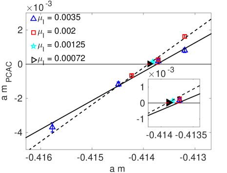
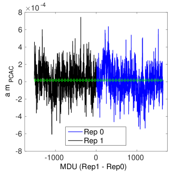
For the tuning process of , which is a function of the light, strange and charm quark mass parameters, we use the and lattices, see section 3.2. for more details. The dependence of the PCAC quark mass on at fixed light twisted mass parameter is shown in Fig. 1. Note that it can be assumed that eq. (8) is valid here for the range i.e. . Using simple linear fits for the ensembles, we determine a critical value of , . We then employ this -value for our large volume ensembles.
For the simulations on the lattices we first thermalize one configuration using 500 trajectories. We then use this configuration as a starting point for two replicas, each having a final statistics of about 1500 MDUs. In Fig. 1 we depict the Monte Carlo history of the PCAC quark mass for these two replicas, where we show, for better visibility, one history plotted by reversed history. The PCAC quark mass fluctuates around zero and does not show particularly large autocorrelation times nor any indication of a first order Sharpe-Singleton transition. Performing the average over the two replica runs, we find . Thus, the condition of eq. (7) is nicely fulfilled. Note that here we do not include the renormalization factor . However, our first estimate is that and anyhow smaller than one, making the condition even better fulfilled. We therefore conclude that the tuning to maximal twist is achieved for the setup. And, as we will demonstrate below, the parameters of the cB211.072.64 runs are chosen such that we indeed simulate at, or very close to the physical values of the pion, the kaon and the D-meson masses.
3.2 Tuning of the heavy quark sector
In tuning the mass parameters of the heavy quark sector we exploit the fact that the value of the critical hopping parameter, as determined in the light quark sector, can be employed also for the heavy quark action while preserving automatic -improvement of all physical observables [3, 50]. Nevertheless, tuning the heavy twisted mass parameters to reproduce the physical values of the strange and charm quark masses is a non-trivial task, owing to the flavour violation [15] inherent to the heavy sector fermion action in eq. (4). In order to tackle the problem, it is convenient to employ in an intermediate step the so-called Osterwalder Seiler (OS) fermions [51] in the valence which avoids these mixing effects. The OS-fermions can be used in a well defined mixed action setup as valence fermions at maximal twist with the same critical mass, , as determined in the unitary setup [3]. The flavour diagonal action, denoted as Osterwalder Seiler fermion action, is given by
| (9) |
with a single-flavour fermion field. The renormalized valence masses can be matched to the corresponding renormalized quark masses via
| (10) |
with and denoting the non-singlet pseudoscalar and scalar Wilson fermion quark bilinear renormalization constants. Then correlation functions using OS or unitary valence quarks are equivalent in the continuum. Moreover they still yield improved physical observables.
The general idea to tune the heavy quark twisted mass parameters is to start with an educated guess in the unitary setup and to tune the OS charm and strange valence masses by imposing two suitably chosen physical renormalization conditions. The so determined parameters of the OS action, i.e. for the strange quark and for the charm quark, can then be translated to new heavy quark twisted mass parameters ( and of eq. (4)) via eq. (10), in the unitary setup and, together with a slight retuning of , a new unitary simulation can be performed. With a convenient choice of the physical renormalization conditions, here and (see below), this parameter tuning procedure can be carried out on a non-large lattice (in the present case, ) and at larger than physical up/down quark mass.
In this work, we follow the above described strategy. As physical conditions we choose
| (11) |
where is the -meson mass and the -meson decay constant. The condition has a strong sensitivity to the charm quark mass while fixes the strange-to-charm mass ratio. They show only small residual light quark mass dependence arising from sea quark effects. We expect these conditions to be essentially free from finite-size effects due to the heavy -meson mass. This setup leads indeed to an only small error for the final parameter choices. Details on our measurements of meson masses and decay constants for twisted mass fermions are given in the Appendix A.
As a first step, we work on gauge ensembles produced with around three times larger than the physical up-down average quark mass and with educated guess values of , and . We choose the OS quark masses and such that condition is fulfilled. We then vary the OS quark masses, while maintaining condition , over a broad enough range such that also condition is satisfied within errors.
In a second step, we match the heavy charm and strange twisted mass of the unitary action (4) to the OS fermion quark mass parameters via eq. (10). The value of is directly determined from and , while is fixed by the ratio . The latter can be estimated by adjusting such that the kaon mass evaluated in the unitary formulation () and its counterpart computed with valence OS fermions () are equal. Although the kaon mass value can be unphysical due to having a too large value of and possible finite size effects, the matching condition actually relates only heavy quark action parameters. It fixes the relation of to and , or equivalently the ratio . In that way it is insensitive to both the finite lattice size and the actual value of up to artifacts. Since the matching steps described so far were implemented only on the valence quark mass parameters of the unitary and OS actions using gauge ensembles with so far different values of the sea quark mass parameters, one still needs to generate new gauge configurations at the so-determined values of and . Now on these new ensembles it can be re-checked whether the condition and the matching condition , as well as the maximal twist condition eq. (7) in the light quark sectors, are fulfilled with sufficient accuracy. If this happens not to be the case, the procedure has to be iterated.
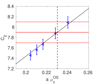
More concretely, we start with an initial guess for the heavy quark mass parameters given by and , which we deduce from a number of tuning runs on a lattice of size and along the lines of ref. [52]. These parameters are realized for the ensemble Th1.200.32.k2, which is moreover very close to maximal twist. We then employ OS fermions in the valence sector and vary the values of and –while maintaining condition – such that condition is fulfilled. This is illustrated in Fig. 2 for the Th1.200.32.k2 ensemble. By requiring that condition is exactly fulfilled, we then fix the values of and , finding
| (12) |
As explained above, the values in eq. (12) already determine . To determine , we first compute the kaon mass in the OS setup at used in the unitary setup and from eq. (12). Having found the OS kaon mass, we go back to the ensemble Th1.200.32.k2 and tune in the unitary heavy quark valence sector such that we match the OS kaon mass. We then take the so found value of and for our simulations on the target large volume lattice. In this process a useful guidance is provided by assuming known to be a typical value from our previous simulations. As we will discuss later, this assumption for turns out to be rather close to the values we determine on the cB211.072.64 ensembles. Our final result for the action parameters in the heavy sector of maximally twisted mass fermions then read
| (13) |
Due to the retuning of the heavy quark masses has to be re-tuned as well. To this end, several ensembles with volumes of at light twisted mass values of and were generated to determine the critical hopping parameter for the simulation at resulting in .
In this work, it turned out that we only needed one iteration of the above procedure using the Th1.200.32.k2 ensemble. After this first step, the tuning conditions for the heavy quark masses were checked again on the Th2.200.32.k2 ensemble (see table 2) and found to hold to a good accuracy within statistical errors. A similar finding holds also on our target ensemble cB211.072.64 ensembles. If we impose again an exact matching between and the unitary on the two cB211.072.64 ensembles we find the ratio of the pseudoscalar to the scalar renormalization constants to be
| (14) |
Using this value of the values of of eq. (13) are close to the corresponding parameters at the physical point (the cB211.072.64 ensembles) that match our tuning conditions. Indeed the actually employed sea quark mass parameters correspond to a sea strange (charm) quark mass lighter ( heavier) than those derived a posteriori from imposing the same tuning and matching conditions on the physical point ensembles. It is also very nice to observe that by enforcing these conditions with very high precision one would obtain at the physical point with fm a kaon mass in isosymmetric QCD less than smaller than its experimental value.
3.3 isospin-breaking lattice artifacts in the pion sector
An important aspect when working with twisted mass fermions at maximal twist is to keep the size of isospin violations small. This isospin breaking manifests itself by the fact that the neutral pion mass becomes lighter than the one of the charged pion. In leading order (LO) of chiral perturbation theory this effect is described by
| (15) |
with the twisted mass angle given by and a low energy constant characterizing the strength of -effects of twisted mass fermions. As shown in Ref. [5, 18], using a clover term the value of the low energy constant decreases. Indeed, employing a clover term, simulations at physical quark masses become possible as demonstrated in Ref. [5]. It turns out that for twisted mass fermions [53] leading to the the Sharpe-Singleton scenario [41].
In order to calculate the neutral pion mass one needs to compute disconnected two-point functions that are notoriously noisy. To suppress the noise in the computation of the two-point functions we use a combination of exact deflation, projecting out the 200 lowest lying eigenvalues, and 6144 stochastic volume sources corresponding to an eight-distance hierarchical probing [54, 55]. The disconnected correlator needed is given by
| (16) |
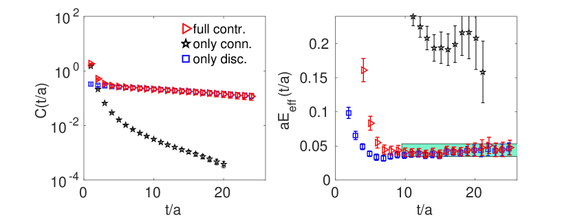
where the ensemble and time average of the vacuum contribution is subtracted from the disconnected operator. Note that we used global volume noise sources to extract the disconnected contribution, however methods which do not subtract the vacuum expectation value explicitly could be more effective as pointed out in [5, 6, 56]. We have found that the disconnected contribution dominates the correlator for time distances , as can be seen in Fig. 3. However we include the connected contribution in the plateau average, leading to a neutral pion mass given by
| (17) |
Note, that for the connected contribution small statistics of around 250 measurements is used, which results in a relatively large statistical error. The charged pion mass is straight forward to compute and we find for the charged pion mass . This gives an isospin splitting in the pion mass of and the low energy constant of eq. (15) reads
| (18) |
assuming . Thus, introducing a clover term for twisted mass fermions suppresses isospin breaking effects effectively, i.e. by a factor of compared to an ensembles with twisted mass fermions without a clover term and a pion mass of 260 MeV at a similar lattice spacing of [53, 57], where it was found that the mass splitting is given by . The suppression of the pion isospin breaking effects, thanks to the use of the clover term, is the underlying reason why we can perform our simulations at the physical point with flavours of quarks.
4 Pseudoscalar meson sector
In order to check, whether we are indeed at (or close to) the targeted physical situation, we studied the charged pion, the kaon and the D-meson masses and decay constants. These observables are rather straightforward to compute with good accuracy. A detailed description of the calculation of these quantities with twisted mass fermions can be found in appendix A .
4.1 Light Meson sector
The first goal of this section is to determine the value of the lattice spacing within the pion sector. The extracted value will then be compared to the one from a similar investigation in the nucleon sector in section 5. In principle, the lattice spacing could be determined already from our cB211.072.64 target ensembles given in Table 2, having a twisted mass parameter of and yielding a pion mass to decay constant ratio of , which is rather close to the physical one. However, it is helpful to also use other ensembles, listed in Table 2, which are all tuned to maximal twist, namely Th1.350.24.k2, Th2.200.32.k2, Th2.150.32.k2 in addition to the cB211.072.64 ensembles. By employing chiral perturbation theory (PT) to describe the quark mass dependence of the pion decay constant and pion mass, we obtain a robust result for the value of the lattice spacing. Since the ensembles that are not at the physical point have partly only a small volume, we include finite volume corrections from chiral perturbation theory to the PT formulae used [58]. We depict in Fig. 4 the ratio and the pion decay constant itself as function of the light bare twisted quark mass.
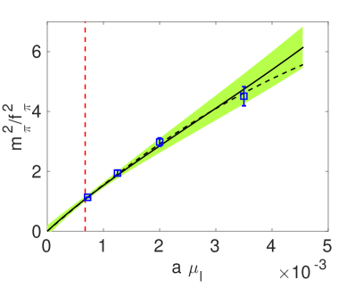
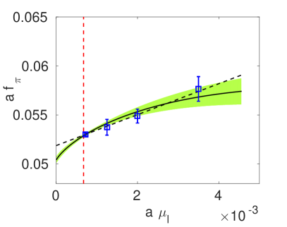
In Fig. 4 we also show the fits to NLO PT [60, 61, 62], which for the ratio read
| (19) |
and for the pion decay constant
| (20) |
with the finite volume correction terms [58]. Here where and are low energy constants. From the fits, we determine the values of and . The fitting constants are related to the NLO low energy constants by
| (21) |
We determine the finite volume correction terms by fixing the low energy constants using the results of Ref. [38]. For our target ensemble cB211.072.64 with we find that the finite volume effects yield corrections of less than for the pion mass and less than for the pion decay constant. By using the fit functions from PT and fixing the ratio we find for the light twisted mass parameter . We then use this value in eq. (20) to determine the lattice spacing. We get
| (22) |
with the first error the statistical and the second the systematic by using the physical value of the pion decay constant, [63]. We follow the procedure adopted in Ref. [39] for determining a systematic error by performing several different fits, adding or neglecting finite volume terms. Such fits employ e.g. the finite volume corrections of Ref. [59] using the calculated low energy constant of eq. (18) different orders in chiral perturbation theory and including or excluding the ensemble Th2.150.32.k2 due to larger finite size effects. The systematic error is then given by the deviations of these different fits from the central value given in eq. (22). Although we include ensembles like Th2.150.32.k2 or Th1.350.24.k2 which have large finite size effect of up to in the pion decay constant, the systematic uncertainties are suppressed due to the fact that we are using ensembles close to physical quark masses which stabilize the fits. Thus this demonstrates the importance of working at physical quark masses. Moreover this is confirmed by an estimation of the lattice spacing which takes only the pion mass and decay constant from cB211.072.64 into account. Requiring a vanishing pion mass in the chiral limit, the lattice spacing and the physical twisted mass value can be fixed by assuming a linear dependence of on and . The so determined lattice spacing agrees with eq. (22) and reads .
4.2 Heavy meson sector
As discussed in section 3.2, the heavy sea quark parameters used in the simulation are tuned by employing the ensemble Th1.200.32.k2. With these parameters the kaon mass on the cB211.072.64 ensembles is smaller as compared to the OS kaon mass using the parameters of eq. (12). By employing the tuning condition of eq. (11) we therefore re-adjust the OS-parameters and following the tuning procedure of section 3.2, to take the values
| (23) |
for the cB211.072.64 lattices. The OS valence quark parameters are lower by around 2.4% compared to the values determined using the Th1.200.32.k2 ensemble (see eq. (12)). By using the strange to light quark mass ratio reads
| (24) |
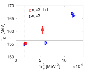
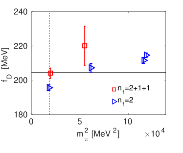
The kaon and D-meson masses and the respective decay constants as well as the corresponding quantities for the -meson are all computed at three different values of and . We use a linear interpolation of , and with respect to the heavy OS quark masses. Using the values for and of eq. (24) this allows us to determine the masses and decay constants for these mesons. In Fig. 5 we show the decay constants of the kaon and the D-meson and compare them with the results extracted from the clover ensembles [5]. We employ 244 measurements for the cB211.072.64 and 100 for the Th2.200.32.k1 ensemble. The ratios of the kaon and D-meson masses to decay constants for the cB211.072.64 ensembles are found to be
| (25) |
where the former ratio has a central value slightly larger than the physical ratio [64], while the latter agrees well within errors with the value [63]. These results indicate that discretization effects for our setup are small in the heavy quark sector. For a more rigorous check, a direct calculation at different values of the lattice spacing will be carried out.
| 0.05658(6) | 0.2014(4) | 0.738(3) | |||
| 1.0731(30) | 3.188(7) | 8.88(11) |
5 Baryon sector
As another test, whether we are in the desired physical condition, we analyzed the nucleon mass which can also provide an independent determination of the lattice spacing, which can be compared to the one found in the meson sector. We measured the nucleon mass on the two cB211.072.64 ensembles by using interpolating fields containing the operator
| (26) |
with the charge conjugation matrix. We then constructed the two point correlation function
| (27) |
which provides the nucleon mass in the large time limit. We used 50 APE smearing steps with [65] in combination with 125 Gaussian smearing steps with [66, 67] to enhance the overlap of the used point sources with the lowest state.
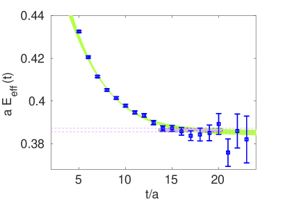
We extracted the nucleon mass for by a plateau average over the effective mass shown in Fig. 6. The plateau average of the nucleon mass, given by on the cB211.072.64 ensemble, is in agreement with a two-state fit with as shown in the left panel of Fig. 6.
5.1 Determination of the lattice spacing
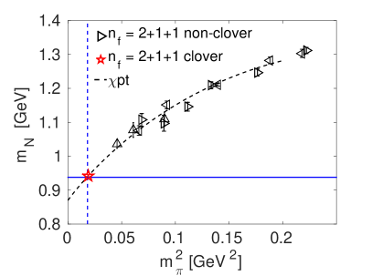
As an alternative way to determine the lattice spacing, one can use the nucleon mass. A direct way would be to use the physical ratio from which, by using the (lattice) pion mass determined above, the lattice spacing can be estimated directly by the value of the lattice nucleon mass. Indeed, with the the pion mass the nucleon to pion mass ratio is close to its physical value of where we take the average of neutron and proton mass [63] and the pion mass in the isospin symmetric limit [64]. However, as in the case of the meson sector, using more data points at heavier pion masses and PT to describe their quark mass dependence, a more robust result can be obtained. More concretely, we have employed chiral perturbation theory at [68, 69] for the nucleon mass dependence on the pion mass, i.e.
| (28) |
Similar to [70] we use the nucleon masses of the ETMC ensembles without a clover term, determined in [71] to perform the chiral fit of eq. (28). In our analysis we neglect cutoff effects, which appear to be small and not visible within our statistical errors. The same holds true for finite volume effects, see [70]. We fixed and [63] in eq. (28). The resulting fit to eq. (28) is shown in Fig. 6 (right) and allows to determine the lattice spacing as
| (29) |
The first error is statistical while the second error is the deviation between the estimate obtained from eq. (28) and taken the mass from the two-state fit. Note that the statistical error in the nucleon mass is comparable with pion sector due to three orders of magnitude larger number of inversions.
5.1.1 isospin splitting in the baryon sector
The finite twisted mass value can result into a mass splitting of hadrons which are symmetric under the isospin symmetry of the light flavor doublet. As pointed out in sec. 3.1 this indeed leads to a sizable effect in the neutral-charged pion mass splitting. Here, we want to discuss the splitting in the baryon sector in case of the -baryon employing the two cB211.072.64 ensembles. Note that for the used lattice size the lowest decay channel of the Delta baryon, which is a nucleon+pion state with correct parity, is heavier than the Delta baryon itself. Thus, for the simulations performed here, the Delta can be treated as a stable state.
We measured the -baryon correlator by using the following interpolating fields
| (30) | |||||
| (31) |
Note that and is symmetric under to and respectively. We neglect the potential mixing of with the spin-1/2 component which is suppressed [72]. Thus the correlators for the is given by with and gives an average value of by using a plateau average over the effective mass. Now we define the splitting in the mass by
| (32) |
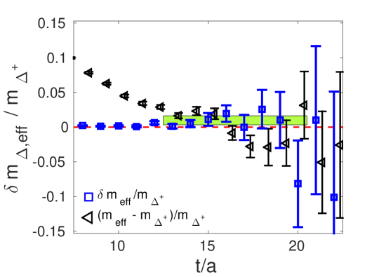
where we average over the symmetric parts. In Fig. 7 we show the effective relative mass splitting given by . In addition we plot the relative effective mass of the particle subtracted from its plateau average to illustrate where the plateau of the -baryon starts. We find that the relative splitting in the mass is and hence close to zero within errors. This result is in agreement with [5] where it was found that the isospin splitting of the twisted mass action in the baryon section is suppressed.
6 Lattice spacing
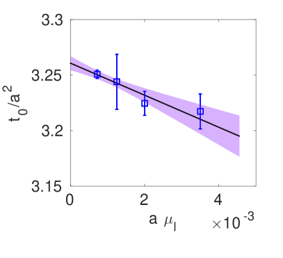
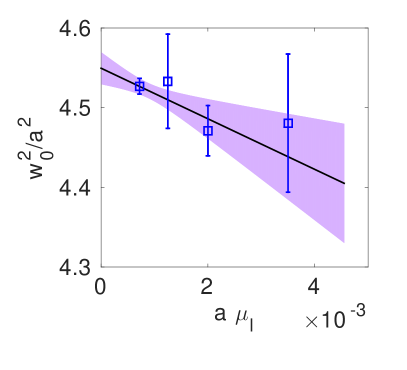
The lattice spacing can be evaluated by matching lattice observables to their physical counterparts. This has been done, as described in sections 4.1 and 5.1, in the meson sector by employing the pion decay constant and in the baryonic sector using the nucleon mass, respectively. Differences in the values obtained for the lattice spacing as determined using different physical observables can shed light on cut-off effects. We discuss in this section an additional method to determine the lattice spacing, which is provided by the gradient flow scale setting parameters [73] and [74]. Following the procedure described in these articles and in particular as applied to the twisted mass setup [5], we extrapolate the gradient flow observables to the chiral limit using a fit ansatz linear in , which corresponds to LO pt [75]. The resulting curve is shown as Fig. 8. We follow a similar procedure for the extrapolation of . We employ the values computed for the ensembles Th1.350.24.k2, Th2.200.32.k2, Th2.125.32.k1, cB211.072.64 and find and . Using the phenomenological values of and [74] we deduce the following values for the lattice spacing
| (33) |
In Table 4 we summarize the values of the lattice spacing as determined from the pion mass and decay constant, the nucleon mass and the gradient flow parameters and . As it can be noticed, there are small deviations of the lattice spacing between the meson and the baryons sector and in any case they are comparable to the one we have observed in the simulations with flavours of quarks. That indicates that cutoff effects do not increase for our flavour setup used here. We would like to stress, that we plan to carry out further simulations at different and, in particular, smaller values of the lattice spacing in future works.
| phys. quant. | lat. spac. [fm] | quantities in lat. units | |
|---|---|---|---|
| 0.0811(14) | |||
| 4.512(16) | |||
| 0.07986(38) | 0.05272(10) | ||
| 0.08087(44) | 6.829(19) | ||
| average | 0.08029(41) |
7 Conclusions
The first successful simulation of maximally twisted mass fermions with quark flavours at the physical values of the pion, the kaon and the D-meson masses has been presented. By having a lattice spacing of , we find that the simulations are stable when performed with physical values of the quark mass parameters. In particular, we are able to carry out a demanding but smooth tuning procedure to maximal twist and to find the values of the light, strange and charm bare quark masses, which correspond to the physical ones for the first two quark generations.
In our setup, which employs a clover term, the cutoff effects appear to be small. Several observations corroborate this conclusion: as already mentioned above, the simulations themselves are very stable; when fixing the quark mass parameters through the selected physical observables, other physical quantities, as collected in Table 3 come out to be consistent with their physical counterparts; the effects originating from the isospin breaking of twisted mass fermions are small and significantly reduced compared to our earlier simulations with flavours at non-physical pion masses; deviations of the lattice spacing from the meson sector, the baryon sector and gradient flow observables, as listed in Table 4, are small and of the same size as in our former flavour simulations.
This work focuses on the tuning procedure both to maximal twist and to the physical values of the quark masses. We include the pseudoscalar meson masses and decay constants as well as the nucleon and masses, in order to demonstrate that we indeed reach the targeted physical setup. We are planning to compute many more quantities in the future connected to hadron structure, scattering phenomena, electroweak observables and heavy quark decay amplitudes. In addition, we have already performed the tuning for a second, finer lattice spacing and we are in the process of generating configurations. The combination of results for various physical quantities from the present lattice spacing of , from the ongoing finer lattice spacing and from an already existing lattice spacing of , which is however not exactly at the physical point, will allow us to explicitly check the size of cut-off effects and eventually take the continuum limit.
We thus conclude that we have given a successful demonstration that simulations of maximally twisted mass fermions with quark flavours can be carried out with all quarks of the first two generations tuned to their physical values. This clearly opens the path for the ETM collaboration to perform simulations towards the continuum limit with a rich research programme being relevant for phenomenology and ongoing and planned experiments.
Acknowledgments
We would like to thank all members of the ETM Collaboration for a productive collaboration. This project has received funding from the Horizon 2020 research and innovation programme of the European Commission under the Marie Sklodowska-Curie grant agreement No 642069. S.B. is supported by this programme. The authors gratefully acknowledge the Gauss Centre for Supercomputing e.V. (www.gauss-centre.eu) for funding the project pr74yo by providing computing time on the GCS Supercomputer SuperMUC at Leibniz Supercomputing Centre (www.lrz.de), where the main simulations were performed. Part of the results were obtained using Piz Daint at Centro Svizzero di Calcolo Scientifico (CSCS), via project with id s702. We thank the staff of LRZ and CSCS for access to the computational resources and for their constant support as well as the Julich Supercomputing Centre (JSC) for the tape storage. Part of this work was supported by the DFG Sino-German CRC110.
Appendix A Mesonic Correlators
In general, the charged 2-point pseudoscalar correlators can be defined by
| (34) |
using the interpolating field
| (35) |
with the quark flavors . For sufficiently large times the charged pseudoscalar correlator is dominated by the lowest energy, such that
| (36) |
and the mass and matrix element can be extracted in a standard way via plateau averages for large time extent. In case of maximal twist the matrix element is directly connected to the pseudoscalar decay constant by [1, 2]
| (37) |
Due to the flavor mixing in case of the mass non-degenerate twisted mass operator we adopt a non-unitary setup [3] for the heavy quark doublet, namely the Osterwalder-Seiler fermion regularization [51]. As shown in [3], this mixed action introduces effects which are only of order and are hence suppressed for small and fine lattice spacings. The OS fermions correspond to the twisted mass discretization in single flavor space, where . The sign of is always chosen such that the two valence quarks in the interpolating fields eq. (35) have opposite signs.
Appendix B Autocorrelation
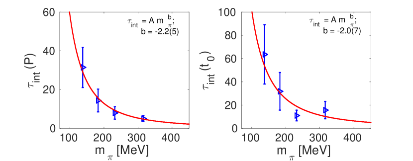
The autocorrelation of the Hybrid Monte Carlo algorithm slows down critically for very fine lattice spacings with . This can be seen in the freezing of the topological charge [77]. For our lattice with we found that the topological charge can fluctuate between the different sectors leading to small autocorrelation times of . As pointed out in [78] the energy density at finite flow times develops larger autocorrelation times in the regime with . Although we have relative small statistics we calculated integrated autocorrelation time for the plaquette and the gradient flow observables as shown in figure 9 by using the -method [79]. We found a pion mass dependence given by
| (38) |
with case of the plaquette while in case of the gradient flow observable . A possible explanation for the quark mass dependence of the autocorrelation time is a phase transition in case of finite twisted mass term for vanishing neutral pion masses. Although the isospin splitting is suppressed in our case, observables like the gradient flow observables shows an increase with inverse of the squared pion mass. This behavior is also seen in the PCAC mass, where moderate integrated autocorrelation times were found which can be clearly seen in the Monte Carlo history (see right panel of fig. 1). However in other quantities like the pseudoscalar mass, the pseudoscalar decay constant or nucleon observables is very small and a quark mass dependence can be not observed.
References
- [1] R. Frezzotti, P. A. Grassi, S. Sint, and P. Weisz. Lattice QCD with a chirally twisted mass term. JHEP, 08:058, 2001.
- [2] R. Frezzotti and G. C. Rossi. Chirally improving Wilson fermions. 1. O(a) improvement. JHEP, 08:007, 2004.
- [3] R. Frezzotti and G. C. Rossi. Chirally improving Wilson fermions. II. Four-quark operators. JHEP, 10:070, 2004.
- [4] A. Abdel-Rehim et al. Nucleon and pion structure with lattice QCD simulations at physical value of the pion mass. Phys. Rev., D92(11):114513, 2015. [Erratum: Phys. Rev.D93,no.3,039904(2016)].
- [5] A. Abdel-Rehim et al. First physics results at the physical pion mass from Wilson twisted mass fermions at maximal twist. Phys. Rev., D95(9):094515, 2017.
- [6] L. Liu et al. Isospin-0 s-wave scattering length from twisted mass lattice QCD. Phys. Rev., D96(5):054516, 2017.
- [7] L. Liu et al. Isospin-0 scattering from twisted mass lattice QCD. PoS, LATTICE2016:119, 2017.
- [8] C. Helmes, B. Knippschild, B. Kostrzewa, L. Liu, C. Jost, K. Ottnad, C. Urbach, U. Wenger, and M. Werner. The meson at the physical point with Wilson twisted mass fermions. In 35th International Symposium on Lattice Field Theory (Lattice 2017) Granada, Spain, June 18-24, 2017, 2017.
- [9] C. Alexandrou et al. Pion vector form factor from lattice QCD at the physical point. Phys. Rev., D97(1):014508, 2018.
- [10] A. Abdel-Rehim, C. Alexandrou, M. Constantinou, K. Hadjiyiannakou, K. Jansen, C. Kallidonis, G. Koutsou, and A. Vaquero Aviles-Casco. Direct Evaluation of the Quark Content of Nucleons from Lattice QCD at the Physical Point. Phys. Rev. Lett., 116(25):252001, 2016.
- [11] C. Alexandrou, M. Constantinou, K. Hadjiyiannakou, K. Jansen, C. Kallidonis, G. Koutsou, and A. Vaquero Aviles-Casco. Nucleon axial form factors using = 2 twisted mass fermions with a physical value of the pion mass. Phys. Rev., D96(5):054507, 2017.
- [12] C. Alexandrou, M. Constantinou, K. Hadjiyiannakou, K. Jansen, C. Kallidonis, G. Koutsou, and A. Vaquero Aviles-Casco. Nucleon electromagnetic form factors using lattice simulations at the physical point. Phys. Rev., D96(3):034503, 2017.
- [13] C. Alexandrou, M. Constantinou, K. Hadjiyiannakou, K. Jansen, C. Kallidonis, G. Koutsou, A. Vaquero Avilés-Casco, and C. Wiese. Nucleon Spin and Momentum Decomposition Using Lattice QCD Simulations. Phys. Rev. Lett., 119(14):142002, 2017.
- [14] C. Alexandrou, S. Bacchio, K. Cichy, M. Constantinou, K. Hadjiyiannakou, K. Jansen, G. Koutsou, A. Scapellato, and F. Steffens. Computation of parton distributions from the quasi-PDF approach at the physical point. In 35th International Symposium on Lattice Field Theory (Lattice 2017) Granada, Spain, June 18-24, 2017, 2017.
- [15] R. Frezzotti and G. C. Rossi. Twisted mass lattice QCD with mass nondegenerate quarks. Nucl. Phys. Proc. Suppl., 128:193–202, 2004. [,193(2003)].
- [16] Y. Iwasaki. Renormalization Group Analysis of Lattice Theories and Improved Lattice Action: Two-Dimensional Nonlinear O(N) Sigma Model. Nucl. Phys., B258:141–156, 1985.
- [17] B. Sheikholeslami and R. Wohlert. Improved Continuum Limit Lattice Action for QCD with Wilson Fermions. Nucl. Phys., B259:572, 1985.
- [18] D. Becirevic, P. Boucaud, V. Lubicz, G. Martinelli, F. Mescia, S. Simula, and C. Tarantino. Exploring twisted mass lattice QCD with the Clover term. Phys. Rev., D74:034501, 2006.
- [19] P. Dimopoulos, H. Simma, and A. Vladikas. Quenched B(K)-parameter from Osterwalder-Seiler tmQCD quarks and mass-splitting discretization effects. JHEP, 07:007, 2009.
- [20] J. Finkenrath, C. Alexandrou, S. Bacchio, P. Charalambous, P. Dimopoulos, R. Frezzotti, K. Jansen, B. Kostrzewa, G. Rossi, and C. Urbach. Simulation of an ensemble of twisted mass clover-improved fermions at physical quark masses. EPJ Web Conf., 175:02003, 2018.
- [21] S. Aoki, R. Frezzotti, and P. Weisz. Computation of the improvement coefficient c(SW) to one loop with improved gluon actions. Nucl. Phys., B540:501–519, 1999.
- [22] S. A. Gottlieb, W. Liu, D. Toussaint, R. L. Renken, and R. L. Sugar. Hybrid molecular dynamics algorithms for the numerical simulation of quantum chromodynamics. Phys. Rev., D35:2531–2542, 1987.
- [23] S. Duane, A. D. Kennedy, B. J. Pendleton, and D. Roweth. Hybrid monte carlo. Phys. Lett., B195:216–222, 1987.
- [24] C. Urbach, K. Jansen, A. Shindler, and U. Wenger. HMC algorithm with multiple time scale integration and mass preconditioning. Comput. Phys. Commun., 174:87–98, 2006.
- [25] K. Jansen and C. Urbach. tmLQCD: A program suite to simulate Wilson twisted mass lattice QCD. Comput. Phys. Commun., 180:2717–2738, 2009.
- [26] M. Hasenbusch. Speeding up the hybrid Monte Carlo algorithm for dynamical fermions. Phys. Lett., B519:177–182, 2001.
- [27] M. Hasenbusch and K. Jansen. Speeding up lattice QCD simulations with clover improved Wilson fermions. Nucl. Phys., B659:299–320, 2003.
- [28] M. A. Clark and A. D. Kennedy. Accelerating dynamical fermion computations using the rational hybrid Monte Carlo (RHMC) algorithm with multiple pseudofermion fields. Phys. Rev. Lett., 98:051601, 2007.
- [29] M. Lüscher. Computational Strategies in Lattice QCD. In Modern perspectives in lattice QCD: Quantum field theory and high performance computing. Proceedings, International School, 93rd Session, Les Houches, France, August 3-28, 2009, pages 331–399, 2010.
- [30] A. Frommer, K. Kahl, S. Krieg, B. Leder, and M. Rottmann. Adaptive Aggregation Based Domain Decomposition Multigrid for the Lattice Wilson Dirac Operator. SIAM J. Sci. Comput., 36:A1581–A1608, 2014.
- [31] C. Alexandrou, S. Bacchio, J. Finkenrath, A. Frommer, K. Kahl, and M. Rottmann. Adaptive Aggregation-based Domain Decomposition Multigrid for Twisted Mass Fermions. Phys. Rev., D94(11):114509, 2016.
- [32] S. Bacchio, C. Alexandrou, and J. Finkenrath. Multigrid accelerated simulations for Twisted Mass fermions. EPJ Web Conf., 175:02002, 2018.
- [33] C. Alexandrou, S. Bacchio, and J. Finkenrath. Multigrid approach in shifted linear systems for the non-degenerated twisted mass operator. 2018.
- [34] C. Urbach. Reversibility Violation in the Hybrid Monte Carlo Algorithm. Comput. Phys. Commun., 224:44–51, 2018.
- [35] R. Frezzotti, G. Martinelli, M. Papinutto, and G. C. Rossi. Reducing cutoff effects in maximally twisted lattice QCD close to the chiral limit. JHEP, 04:038, 2006.
- [36] K. Jansen, M. Papinutto, A. Shindler, C. Urbach, and I. Wetzorke. Quenched scaling of Wilson twisted mass fermions. JHEP, 09:071, 2005.
- [37] R. Baron et al. Computing K and D meson masses with = 2+1+1 twisted mass lattice QCD. Comput. Phys. Commun., 182:299–316, 2011.
- [38] N. Carrasco et al. Up, down, strange and charm quark masses with Nf = 2+1+1 twisted mass lattice QCD. Nucl. Phys., B887:19–68, 2014.
- [39] P. Boucaud et al. Dynamical Twisted Mass Fermions with Light Quarks: Simulation and Analysis Details. Comput. Phys. Commun., 179:695–715, 2008.
- [40] S. Aoki and O. Bar. Twisted-mass QCD, O(a) improvement and Wilson chiral perturbation theory. Phys. Rev., D70:116011, 2004.
- [41] S. R. Sharpe and Robert L. Singleton, Jr. Spontaneous flavor and parity breaking with Wilson fermions. Phys. Rev., D58:074501, 1998.
- [42] O. Janssen, M. Kieburg, K. Splittorff, J. J. M. Verbaarschot, and S. Zafeiropoulos. Phase Diagram of Dynamical Twisted Mass Wilson Fermions at Finite Isospin Chemical Potential. Phys. Rev., D93(9):094502, 2016.
- [43] S. R. Sharpe. Observations on discretization errors in twisted-mass lattice QCD. Phys. Rev., D72:074510, 2005.
- [44] F. Farchioni et al. Twisted mass quarks and the phase structure of lattice QCD. Eur. Phys. J., C39:421–433, 2005.
- [45] F. Farchioni et al. Exploring the phase structure of lattice QCD with twisted mass quarks. Nucl. Phys. Proc. Suppl., 140:240–245, 2005.
- [46] F. Farchioni et al. The phase structure of lattice QCD with Wilson quarks and renormalization group improved gluons. Eur. Phys. J., C42:73–87, 2005.
- [47] F. Farchioni et al. Dynamical twisted mass fermions. PoS, LAT2005:072, 2006.
- [48] F. Farchioni et al. Numerical simulations with two flavors of twisted-mass Wilson quarks and DBW2 gauge action. Eur. Phys. J., C47:453–472, 2006.
- [49] F. Farchioni et al. Lattice spacing dependence of the first order phase transition for dynamical twisted mass fermions. Phys. Lett., B624:324–333, 2005.
- [50] T. Chiarappa, F. Farchioni, K. Jansen, I. Montvay, E. E. Scholz, L. Scorzato, T. Sudmann, and C. Urbach. Numerical simulation of QCD with u, d, s and c quarks in the twisted-mass Wilson formulation. Eur. Phys. J., C50:373–383, 2007.
- [51] K. Osterwalder and E. Seiler. Gauge Field Theories on the Lattice. Annals Phys., 110:440, 1978.
- [52] A. Abdel-Rehim et al. Progress in Simulations with Twisted Mass Fermions at the Physical Point. PoS, LATTICE2014:119, 2015.
- [53] G. Herdoiza, K. Jansen, C. Michael, K. Ottnad, and C. Urbach. Determination of Low-Energy Constants of Wilson Chiral Perturbation Theory. JHEP, 05:038, 2013.
- [54] A. Stathopoulos, J. Laeuchli, and K. Orginos. Hierarchical probing for estimating the trace of the matrix inverse on toroidal lattices. 2013.
- [55] Ab. Abdel-Rehim, C. Alexandrou, M. Constantinou, J. Finkenrath, K. Hadjiyiannakou, K. Jansen, C. Kallidonis, G. Koutsou, A. V. Avilés-Casco, and J. Volmer. Disconnected diagrams with twisted-mass fermions. PoS, LATTICE2016:155, 2016.
- [56] K. Ottnad and C. Urbach. Flavor-singlet meson decay constants from twisted mass lattice QCD. Phys. Rev., D97(5):054508, 2018.
- [57] R. Baron et al. Light hadrons from lattice QCD with light (u,d), strange and charm dynamical quarks. JHEP, 06:111, 2010.
- [58] G. Colangelo, S. Dürr, and C. Haefeli. Finite volume effects for meson masses and decay constants. Nucl. Phys., B721:136–174, 2005.
- [59] G. Colangelo, U. Wenger, and J. M. S. Wu. Twisted Mass Finite Volume Effects. Phys. Rev., D82:034502, 2010.
- [60] S. Weinberg. Phenomenological Lagrangians. Physica, A96:327–340, 1979.
- [61] J. Gasser and H. Leutwyler. Chiral Perturbation Theory to One Loop. Annals Phys., 158:142, 1984.
- [62] J. Gasser and H. Leutwyler. Chiral Perturbation Theory: Expansions in the Mass of the Strange Quark. Nucl. Phys., B250:465–516, 1985.
- [63] C. Patrignani et al. Review of Particle Physics. Chin. Phys., C40(10):100001, 2016.
- [64] S. Aoki et al. Review of lattice results concerning low-energy particle physics. Eur. Phys. J., C77(2):112, 2017.
- [65] M. Albanese et al. Glueball Masses and String Tension in Lattice QCD. Phys. Lett., B192:163–169, 1987.
- [66] S. Gusken. A Study of smearing techniques for hadron correlation functions. Nucl. Phys. Proc. Suppl., 17:361–364, 1990.
- [67] C. Alexandrou, S. Gusken, F. Jegerlehner, K. Schilling, and R. Sommer. The Static approximation of heavy - light quark systems: A Systematic lattice study. Nucl. Phys., B414:815–855, 1994.
- [68] J. Gasser, M. E. Sainio, and A. Svarc. Nucleons with Chiral Loops. Nucl. Phys., B307:779–853, 1988.
- [69] B. C. Tiburzi and A. Walker-Loud. Hyperons in Two Flavor Chiral Perturbation Theory. Phys. Lett., B669:246–253, 2008.
- [70] C. Alexandrou and C. Kallidonis. Low-lying baryon masses using twisted mass clover-improved fermions directly at the physical pion mass. Phys. Rev., D96(3):034511, 2017.
- [71] C. Alexandrou, V. Drach, K. Jansen, C. Kallidonis, and G. Koutsou. Baryon spectrum with twisted mass fermions. Phys. Rev., D90(7):074501, 2014.
- [72] C. Alexandrou et al. Light baryon masses with dynamical twisted mass fermions. Phys. Rev., D78:014509, 2008.
- [73] M. Lüscher. Properties and uses of the Wilson flow in lattice QCD. JHEP, 08:071, 2010. [Erratum: JHEP03,092(2014)].
- [74] S. Borsanyi et al. High-precision scale setting in lattice QCD. JHEP, 09:010, 2012.
- [75] O. Bar and M. Golterman. Chiral perturbation theory for gradient flow observables. Phys. Rev., D89(3):034505, 2014. [Erratum: Phys. Rev.D89,no.9,099905(2014)].
- [76] M. Schmelling. Averaging correlated data. Physica Scripta, 51(6):676, 1995.
- [77] S. Schaefer, R. Sommer, and F. Virotta. Critical slowing down and error analysis in lattice QCD simulations. Nucl. Phys., B845:93–119, 2011.
- [78] M. Bruno, S. Schaefer, and R. Sommer. Topological susceptibility and the sampling of field space in Nf = 2 lattice QCD simulations. JHEP, 08:150, 2014.
- [79] U. Wolff. Monte Carlo errors with less errors. Comput. Phys. Commun., 156:143–153, 2004. [Erratum: Comput. Phys. Commun.176,383(2007)].