Effects of quantum statistics on relic density
of Dark Radiation

Marek Olechowski, Paweł Szczerbiak

Institute of Theoretical Physics, Faculty of Physics, University of Warsaw

ul. Pasteura 5, PL–02–093 Warsaw, Poland

Abstract

The freeze-out of massless particles is investigated. The effects due to quantum statistics, Fermi-Dirac or Bose-Einstein, of all particles relevant for the process are analyzed. Solutions of appropriate Boltzmann equation are compared with those obtained using some popular approximate methods. As an application of general results the relic density of dark radiation in Weinberg’s Higgs portal model is discussed.

1 Introduction

In recent decades the cosmic microwave background radiation has been extensively analyzed, unveiling many crucial facts about the history of the Universe and its constituents. Although we are convinced that about 27% of the total mass-energy fraction of the Universe consists of presumably cold or warm dark matter, there are still some hints that additional form of dark radiation (DR) – called also hot dark matter – may also exist. According to the recent Planck satellite measurements [1] the effective number of light neutrino species $N_{\rm eff}$ varies (depending on the effects included) from $2.99\pm 0.20$ to $3.15\pm 0.23\;(1\sigma)$, which indicates that both the Standard Model (SM) and models with fractional $\Delta N_{\rm eff}\equiv N_{\rm eff}-N_{\rm eff}^{\rm SM}>0$ are consistent with this result (one fully thermalized neutrino i.e. $\Delta N_{\rm eff}=1$ is ruled out at over 3$\sigma$). On the other hand, the value of the Hubble constant $H_{0}$ obtained from direct observations [2] performed using the Hubble Space Telescope i.e. $73.24\pm 1.74\;\rm km\,s^{-1}Mpc^{-1}$ is significantly bigger than $67.8\pm 0.9\;\rm km\,s^{-1}Mpc^{-1}$ inferred from the Planck data. Such high value of $H_{0}$ favors additional contribution to $\Delta N_{\rm eff}$ (even of order 0.6 [3]), however global fits still prefer the standard $\Lambda$CDM scenario [4]. There is hope that this apparent tension will be clarified in near future, especially with the advent of the CMB-S4 experiment [5] that will be able to probe $\Delta N_{\rm eff}$ with precision better than 0.03. So precise experimental results will require more accurate theoretical treatment of DR freeze-out details than is usually considered in the literature.

One of the most widely studied scenarios predicting an existence of additional form of radiation is the Weinberg’s Higgs portal model [6] in which a massless Nambu-Goldstone boson of a broken global U(1) symmetry gives fractional contribution to $N_{\rm eff}$. It is often assumed that the freeze-out of that boson takes places just before $\mu^{+}\mu^{-}$ annihilation, resulting in $\Delta N_{\rm eff}\approx 0.39$. However, there are some effects, which we discuss in this work, that might strongly influence the Goldstone boson relic density in such case. Moreover, we consider situations when such boson decouples at different temperature. Most of our results may be applied also in other models of DR.

The outline of this work is as follows. In section 2 we discuss the Boltzmann equation describing the freeze-out of a massless particle and some approximate methods used in the literature. Main features of the Weinberg’s Higgs portal model are given in section 3. In section 4 the relic density of DR in this model is analyzed in some detail using the general results presented in section 2. Section 5 contains our main conclusions.

2 Boltzmann equation for massless particles

Boltzmann equation in FLRW metric takes the form

$$E(\partial_{t}-pH\partial_{p})f(p,t)=C_{E}(p,t)+C_{I}(p,t)\,,$$ (1)

where $f(p,t)$ is a distribution function to be found, whereas terms at the RHS are collision integrals for elastic ($E$) and inelastic ($I$) processes. Elastic collisions are responsible for momentum exchange between particles (preserving their relative numbers) and in consequence help to maintain kinetic equilibrium. Inelastic collisions are related to (co)annihilation processes that influence chemical equilibrium.

Elastic processes are usually stronger than inelastic ones, so we will assume here that kinetic equilibrium is maintained. Such assumption is not always valid and under certain circumstances may lead to sizable differences in relic density calculation. There are several methods which are applicable for Boltzmann equation solution without kinetic equilibrium – this problem has been extensively analyzed in the context of neutrino decoupling in the Standard Model. We can distinguish two major classes of relic density calculation for relativistic particles in such a case: discretization in momentum space [7, 8, 9, 10] and spectral methods based on fixed [11, 12] or dynamical [13, 14] basis of orthogonal polynomials. All these approaches allow for high accuracy but at the price of lengthy and complicated expressions that are unpractical for qualitative study. In the present work we are mainly interested in estimation of Bose-Einstein (BE)/Fermi-Dirac (FD) statistics corrections to the relic density for massless particles. Thus, it suffices in our case to perform analysis assuming the kinetic equilibrium.

The collision integral for inelastic processes involving particle $\chi$, $C_{I}(p_{\chi},t)$, with only two-body processes $\chi a\leftrightarrow bc$ taken into account, may be expressed as

$$\begin{split}C_{I}(p_{\chi},t)=\frac{1}{2}\sum_{\{a,b,c\}}\int\prod_{i=a,b,c}&\frac{{\rm d}^{3}p_{i}}{2\pi^{3}E_{i}}(2\pi)^{4}\delta^{(4)}(p_{\chi}+p_{a}-p_{b}-p_{c})\\ \times\sum_{\rm spins}&\left[|M_{bc\rightarrow\chi a}|^{2}f_{b}(p_{b},t){f}_{c}(p_{c},t)(1-f_{\chi}(p_{\chi},t))(1-{f}_{a}(p_{a},t))\right.\\ &-\left.|M_{\chi a\rightarrow bc}|^{2}f_{\chi}(p_{\chi},t){f}_{a}(p_{a},t)(1-f_{b}(p_{b},t))(1-{f}_{c}(p_{c},t))\right]\,,\end{split}$$ (2)

where the sum over $\{a,b,c\}$ corresponds to all allowed processes $\chi a\leftrightarrow bc$. We will calculate the above collision integral exploiting the method proposed in [15], where the effect of FD statistics was analyzed in the context of relic density calculation for relativistic fermions ($0\not=m\ll T_{f}$) staying in kinetic equilibrium. Below we will focus on annihilation of massless particles (bosons and fermions) including full statistics for both initial and final states. The results will be used in section 4 to analyze the Goldstone bosons freeze-out in the Weinberg’s Higgs portal model.

Let us consider annihilation process of the form $\bar{\chi}\chi\to\bar{N}N$, where $N$ stays in kinetic and chemical equilibrium during $\chi$ freeze-out. For definiteness, we will focus on one process of this kind (generalization is straightforward). Distribution functions for $\chi$ and $N$ may be written in the form

$$f_{\chi}(p,t)\simeq\left(e^{E/T+z}\mp 1\right)^{-1}\equiv\left(e^{xy+z}+s_{\rm in}\right)^{-1}\,,$$ (3)

$$f_{N}(p,t)\simeq\left(e^{E_{N}/T}+s_{\rm out}\right)^{-1}\,,$$ (4)

where $z=z(t)$ is the so-called chemical pseudopotential (equal for $\chi$ and $\bar{\chi}$) [16]. We also defined $x\equiv m/T$ and $y\equiv E/m$ (for one massive annihilation product $N$ it is convenient to choose $m\equiv m_{N}\not=0$). The statistical factors $s_{\rm in}$ and $s_{\rm out}$ equal $+1$ and $-1$ for fermions and bosons, respectively – by setting these factors to zero one obtains the Maxwell-Boltzmann (MB) approximation. Using the above definitions and integrating expression (2) over $\chi$ momenta one may rewrite eq. (1) in the following form [15]

$$\frac{{\rm d}z}{{\rm d}x}\simeq\left(A(z,x)\frac{x}{T}\frac{{\rm d}T}{{\rm d}t}\right)^{-1}\left(S_{I}(z,x)-B(z,x)\right)\,,$$ (5)

where

$$\begin{split}A(z,x)&\equiv\frac{g}{2\pi^{2}}m^{3}e^{z}J_{2}(z,x)\,,\\ B(z,x)&\equiv\frac{g}{2\pi^{2}}m^{3}e^{z}xJ_{3}(z,x)H(x)\left(1-\frac{1}{1-\frac{x}{3}\frac{g_{*s}^{\prime}(x)}{g_{*s}(x)}}\right)\,,\\ S_{I}(z,x)&\equiv\int\frac{{\rm d}^{3}p}{(2\pi)^{3}}\frac{1}{E}C_{I}(p,t)\,,\end{split}$$ (6)

$g$ is the number of $\chi$ degrees of freedom, the Hubble parameter is given by

$$H(x)=\sqrt{\frac{4\pi^{3}}{45}}\sqrt{g_{*}(x)}\frac{m^{2}}{M_{\rm Pl}}\frac{1}{x^{2}}\,,$$ (7)

and

$$J_{n}(z,x)\equiv\int_{0}^{\infty}{\rm d}y\,y^{n}\frac{e^{xy}}{(e^{xy+z}+s_{\rm in})^{2}}\;.$$ (8)

The most elaborate part is the calculation of the collision integral $S_{I}$ which, after using four-momentum conservation, is 5-dimensional. We use the following convenient set of variables: energies of the incoming particles, $E_{1}$ and $E_{2}$, one of the outgoing particles’ energy, $E_{3}$, the angle between momenta of the incoming particles, $\theta$, and the acoplanarity angle $\phi$. Defining dimensionless parameters $u\equiv E_{1}/m$, $v\equiv E_{2}/m$ and $t\equiv E_{3}/m$ one can write

$$S_{I}(z,x)=\frac{m^{4}}{512\pi^{6}}\left(e^{2z}-1\right)\int\mathscr{D}\Phi\int_{0}^{2\pi}{\rm d}\phi\sum_{\rm spins}|M_{\chi\bar{\chi}\to N\bar{N}}(u,v,t,\cos\theta,\phi)|^{2}\,,$$ (9)

where

$$\begin{split}\mathscr{D}\Phi&\equiv\int_{0}^{\infty}{\rm d}u\int_{0}^{\infty}{\rm d}v\int_{-1}^{1}{\rm d}\cos\theta\frac{uv\,e^{x(u+v)}}{\kappa(u,v,\theta)}\int_{t_{-}}^{t_{+}}{\rm d}t\\ &\times\frac{1}{\left(e^{xu+z}+s_{\rm in}\right)\left(e^{xv+z}+s_{\rm in}\right)\left(e^{xt}+s_{\rm out}\right)\left(e^{x(u+v-t)}+s_{\rm out}\right)}\end{split}$$ (10)

and we introduced the following functions of the parameters: $\kappa(u,v,\theta)\equiv(u^{2}+v^{2}+2\,uv\cos\theta)^{1/2}$, $V(u,v,\theta)\equiv(1-4m^{2}/s)^{1/2}$, $t_{\pm}\equiv\frac{1}{2}\left[u+v\pm\kappa(u,v,\theta)V(u,v,\theta)\right]$. If (which is often the case in leading approximation) $M_{\chi\bar{\chi}\to N\bar{N}}$ depends only on $s$ (given here by $s=2uv\,m^{2}(1-\cos\theta)$), introducing new combinations of the parameters $p=x(u+v)$ and $q=x\sqrt{u^{2}+v^{2}+2uv\cos\theta}$, we can reduce the above integral to

$$\begin{split}\mathscr{D}\Phi&=\frac{1}{x^{4}}\int_{2x}^{\infty}{\rm d}p\int_{0}^{\sqrt{p^{2}-4x^{2}}}{\rm d}q\;\frac{1}{(|s_{\rm out}|-e^{-p})(e^{p+2z}-|s_{\rm out}|)}\\ &\times\ln\left[\frac{\cosh\left(\frac{1}{2}(p+q)+z\right)+s_{\rm in}}{\cosh\left(\frac{1}{2}(p-q)+z\right)+s_{\rm in}}\right]\ln\left[\frac{\cosh\left(\frac{1}{2}\big{(}p+qV(p,q)\big{)}\right)+s_{\rm out}}{\cosh\left(\frac{1}{2}\big{(}p-qV(p,q)\big{)}\right)+s_{\rm out}}\right]\,,\end{split}$$ (11)

where now $V=\left(1-\frac{4x^{2}}{p^{2}-q^{2}}\right)^{1/2}$ and $s=\frac{p^{2}-q^{2}}{x^{2}}m^{2}$. In such a case the integration over $\phi$ in eq. (9) is trivial and the expression simplifies. Then, the Boltzmann equation (5) may be written in the following integro-differential form

$$\frac{{\rm d}z}{{\rm d}x}=-\frac{x}{J_{2}(z,x)}\left(\frac{1}{3}\frac{g^{\prime}_{*s}(x)}{g_{*s}(x)}J_{3}(z,x)+\frac{\sqrt{45}}{256\pi^{11/2}}\frac{M_{\rm Pl}}{m}\frac{\sinh z}{g\sqrt{g_{*}(x)}}\left(1-\frac{x}{3}\frac{g^{\prime}_{*s}(x)}{g_{*s}(x)}\right)\tilde{S}_{I}(z,x)\right)\,.$$ (12)

Note that we introduced dimensionless (in contrast to $S_{I}(z,x)$) collision integral (see eq. (11))

$$\tilde{S}_{I}(z,x)=2\pi\int\mathscr{D}\Phi\sum_{\rm spins}|M_{\chi\bar{\chi}\to N\bar{N}}(s)|^{2}\,.$$ (13)

The number density of $\chi$ ($=\bar{\chi}$) may be easily found after integration over the whole energy range

$$n(x)\equiv n_{\chi}(x)=g\frac{m^{3}}{2\pi^{2}}\int_{0}^{\infty}\frac{y^{2}{\rm d}y}{e^{xy+z}+s_{\rm in}}\;.$$ (14)

2.1 MB approximation and limited inclusion of BE/FD statistics

Let us consider the particle number density normalized by the entropy density: $Y(x)\equiv\frac{n(x)}{s(x)}$. In chemical and kinetic equilibrium (subscript eq) we just have (using eq. (14) with $z=0$)

$$Y_{\rm eq}(x)=g\,\frac{45}{2\pi^{4}}\frac{\zeta^{\rm in}}{g_{*s}(x)}\;,$$ (15)

where

$$\zeta^{\rm in}\equiv\zeta(3)\begin{cases}1&\text{BE}\\ 3/4&\text{FD}\end{cases}\,.$$ (16)

For the Maxwell-Boltzmann statistics one can write

$$Y(x)=e^{-z}Y_{\rm eq}(x)\,.$$ (17)

Then, the Boltzmann equation (12) simplifies to (we use $s_{\rm in}=s_{\rm out}=0$ in eqs. (8) and (10))

$$\frac{{\rm d}z}{{\rm d}x}=\ -\frac{g^{\prime}_{*s}(x)}{g_{*s}(x)}-\frac{\sqrt{45}}{\pi^{7/2}}\frac{M_{\rm Pl}m}{x^{2}}\frac{\sinh z}{g\sqrt{g_{*}(x)}}\left(1-\frac{x}{3}\frac{g_{*s}^{\prime}(x)}{g_{*s}(\tilde{x})}\right)\langle\sigma v\rangle_{\rm MB}\;.$$ (18)

One can also rewrite it in the Lee-Weinberg form

$$Y^{\prime}(x)=-\sqrt{\frac{\pi}{45}}\frac{g_{*s}(x)}{\sqrt{g_{*}(x)}}\frac{M_{\rm Pl}m}{x^{2}}\left(Y^{2}(x)-Y^{2}_{\rm eq}(x)\right)\langle\sigma v\rangle_{\rm MB}\frac{1}{\zeta^{\rm in}}\;,$$ (19)

where $v$ is the Möller velocity for the incoming particles and

$$\langle\sigma v\rangle_{\rm MB}=\frac{1}{512\pi}\frac{x^{5}}{m^{5}}\int_{4m^{2}}^{\infty}{\rm d}s\,\sqrt{s}\,\sqrt{1-\frac{4m^{2}}{s}}\,\sum_{\rm spins}|M(s)|^{2}{\rm K}_{1}\left(\frac{x\sqrt{s}}{m}\right)\,.$$ (20)

Please note the presence of additional factor $1/\zeta^{\rm in}$ in the RHS of eq. (19) as compared to the standard form [17]. It comes from the fact that $Y_{\rm eq}$ contains information about the incoming particles statistics whereas eq. (12), after putting everywhere $s_{\rm out}=s_{\rm in}=0$, does not. Multiplying $\tilde{S}_{I}(z,x)$ by $\zeta^{\rm in}$ one can obtain the familiar Lee-Weinberg equation. Thus, we have two options:

1. Use eqs. (15) and (19) with $\zeta^{\rm in}=1$ (pure MB approximation).

2. Use eqs. (15) and (19) with $\zeta^{\rm in}$ given by eq. (16) in the former but $\zeta^{\rm in}=1$ in the latter (we call it fractional inclusion of BE/FD statistics for incoming particles and denote as fBE/fFD).

One can also include BE/FD statistics (again, only for incoming particles) in thermally averaged cross section

$$\begin{split}\langle\sigma v\rangle_{\rm p}&=\frac{1}{512\pi(\zeta^{\rm in})^{2}}\frac{x^{5}}{m^{5}}\int_{4m^{2}}^{\infty}{\rm d}s\,\sqrt{1-\frac{4m^{2}}{s}}\,\sum_{\rm spins}|M(s)|^{2}\\ &\times\int_{\sqrt{s}}^{\infty}{\rm d}E_{+}\frac{e^{-\frac{x}{2m}E_{+}}}{\sinh\left(\frac{x}{2m}E_{+}\right)}\ln\left[\frac{{\rm fh}\left(\frac{x}{4m}\left(E_{+}+\sqrt{E_{+}^{2}-s}\right)\right)}{{\rm fh}\left(\frac{x}{4m}\left(E_{+}-\sqrt{E_{+}^{2}-s}\right)\right)}\right]\,,\end{split}$$ (21)

where ${\rm fh}$ is a hyperbolic function depending on the statistics of incoming particles: ${\rm fh}\equiv\sinh$ ($\cosh$) for bosons (fermions) and index p stands for partial inclusion of statistics. Thus, we consider another approximate method:

1. The same rules as in the point 2. above but with $\langle\sigma v\rangle_{\rm p}$ (eq. (21)) instead of $\langle\sigma v\rangle_{\rm MB}$ (eq. (20)) (we call it partial inclusion of BE/FD statistics for incoming particles and denote as pBE/pFD).

The main difference between eqs. (11) and (21) is that in the latter case the expression does not depend on $Y$ (or equivalently on $z$), which significantly simplifies calculations. Note also that none of the above approximations include any effect of the outgoing particles statistics.

3 Weinberg’s Higgs portal model

For easy reference we remind here the main features of the model proposed in [6] (using notation mainly from [18]). In addition to the SM fields it contains a dark sector consisting of a complex scalar $\phi$ and a Dirac fermion $\psi$. Both new fields are charged only under a global $U(1)_{\rm dark}$ symmetry with charges: $Q_{\rm dark}(\psi)=1$, $Q_{\rm dark}(\phi)=2$. A non-zero VEV of $\phi$ spontaneously breaks this symmetry to the discrete $\mathbb{Z}_{2}$ parity. The Goldstone boson associated with this symmetry breaking contributes to DR while the lighter dark fermion ($\psi$ gives two Majorana fermions with different masses) is stable and plays the role of cold dark matter (CDM).

We will concentrate here on the scalar sector which is the most important one for our analysis. The corresponding part of the Lagrangian density is given by

$$\begin{split}\mathcal{L}_{H,\phi}=&\left(D_{\mu}H\right)^{\dagger}\left(D^{\mu}H\right)+\mu_{H}^{2}H^{\dagger}H-\lambda_{H}(H^{\dagger}H)^{2}\\ +&\partial_{\mu}\phi^{*}\partial^{\mu}\phi+\mu_{\phi}^{2}(\phi^{*}\phi)^{2}-\lambda_{\phi}(\phi^{*}\phi)^{2}-\kappa(H^{\dagger}H)(\phi^{*}\phi)\;,\end{split}$$ (22)

where $H$ is the Standard Model Higgs doublet. After the spontaneous symmetry breaking the scalar fields may be written as

$$H=\begin{pmatrix}G^{+}\\ v_{H}+\frac{\tilde{h}+iG^{0}}{\sqrt{2}}\end{pmatrix}\;,\quad\quad\phi=v_{\phi}+\frac{\tilde{\rho}+i\sigma}{\sqrt{2}}\;,$$ (23)

where $\sigma$ is the Goldstone boson of the broken $U(1)_{\rm dark}$ and contributes to DR. Two neutral scalars $\tilde{h}$ and $\tilde{\rho}$ mix, forming two mass eigenstates ($h$ and $\rho$):

$$h=\tilde{h}\cos\theta+\tilde{\rho}\sin\theta\;,\quad\quad\rho=\tilde{\rho}\cos\theta-\tilde{h}\sin\theta\;,$$ (24)

with masses

$$m_{h}^{2}=4\lambda_{H}v_{H}^{2}\cos^{2}\theta+4\lambda_{\phi}v_{\phi}^{2}\sin^{2}\theta+2\kappa\,v_{H}v_{\phi}\sin 2\theta\,,$$ (25)

$$m_{\rho}^{2}=4\lambda_{\rho}v_{\rho}^{2}\cos^{2}\theta+4\lambda_{H}v_{H}^{2}\sin^{2}\theta-2\kappa\,v_{H}v_{\phi}\sin 2\theta\,,$$ (26)

and the mixing angle given by the condition

$$\tan 2\theta=\frac{\kappa\,v_{H}v_{\phi}}{\lambda_{H}v_{H}^{2}-\lambda_{\phi}v_{\phi}^{2}}\;.$$ (27)

The scalar potential in (22) depends on five parameters. They must satisfy two conditions in order to give the correct values of $v_{H}$ and the mass of the Higgs particle (identified with $h$). As the three parameters, describing the remaining freedom in the scalar Lagrangian (22), we choose two couplings, $\lambda_{\phi}$ and $\kappa$, and the mass of the non-SM-like scalar, $m_{\rho}$. Other parameters present in the mass formulas (25) and (26) may be expressed as

$$\sin\theta\simeq\frac{\kappa\,m_{\rho}v_{H}}{\left[\lambda_{\phi}(m_{h}^{2}-m_{\rho}^{2})^{2}-\kappa^{2}v_{H}^{2}(m_{h}^{2}-m_{\rho}^{2})\right]^{1/2}}\approx\frac{\kappa}{\lambda_{\phi}^{1/2}}\left(\frac{m_{\rho}}{90\;\,\rm GeV}\right)\;,$$ (28)

$$\lambda_{H}=\frac{m_{h}^{2}\cos^{2}\theta+m_{\rho}^{2}\sin^{2}\theta}{4v_{H}^{2}}\approx 0.13\cos^{2}\theta\;,$$ (29)

$$v_{\phi}^{2}=\frac{m_{\rho}^{2}\cos^{2}\theta+m_{h}^{2}\sin^{2}\theta}{4\lambda_{\phi}}\approx m_{\rho}^{2}\left(\frac{\cos\theta}{2\lambda_{\phi}^{1/2}}\right)^{2}\;,$$ (30)

where the approximate equalities are valid if the scalar $\rho$ is relatively light and does not mix strongly with the SM-like Higgs i.e. $m^{2}_{\rho}\ll m^{2}_{h}$, $\sin^{2}\theta\ll 1$.

Let us now estimate phenomenologically interesting range of values for $\kappa$ and $\lambda_{\phi}$ that will be used in our numerical scan. The contribution from the dark particles to the invisible Higgs decay width may be approximated as

$$\Delta\Gamma_{h,{\rm inv}}\geq\Gamma(h\to\sigma\sigma)+\Gamma(h\to\rho\rho)\approx\frac{\sin^{2}\theta}{32\pi}\frac{m_{h}^{3}}{v_{\phi}^{2}}\approx\frac{\kappa^{2}}{8\pi\cos^{2}\theta}\frac{v_{H}^{2}}{m_{h}}\,,$$ (31)

where we conservatively neglected the Higgs decays into dark fermions. The LHC constraint on the invisible Higgs decays i.e.

$$\Delta\Gamma_{h,{\rm inv}}<\frac{B_{\rm inv}\cos^{2}\theta}{1-B_{\rm inv}}\Gamma_{h,\rm SM}\,,$$ (32)

where $B_{\rm inv}\lesssim 24\%$ [19] and $\Gamma_{h,\rm SM}\simeq 4$ MeV, may be used together with eq. (31) to obtain the following upper bound on the portal coupling:

$$\kappa\lesssim 0.01\,.$$ (33)

Bounds on the singlet scalar self-coupling, $\lambda_{\phi}$, are much weaker. They follow from the requirement of perturbativity to some high energy scale and may be obtained from the RG equations [20]:

$$\begin{split}16\pi^{2}\frac{{\rm d}\lambda_{\phi}}{{\rm d}t}&=10\lambda_{\phi}^{2}+\kappa^{2}\,,\\ 16\pi^{2}\frac{{\rm d}\kappa}{{\rm d}t}&=\kappa\left(2\kappa+4\lambda_{\phi}+6\lambda_{H}+3y_{t}^{2}-\frac{9}{4}g_{2}^{2}-\frac{3}{4}g_{1}^{2}\right)\,,\end{split}$$ (34)

where $t\equiv Q^{2}/Q_{0}^{2}$. The scalar couplings stay perturbative up to the GUT energy scale if at low energy $\lambda_{\phi}\lesssim 0.25$. On the other hand, if $\lambda_{\phi}=1$ at the weak scale, it becomes non-perturbative already at scale of order 100 TeV. Both values i.e. $\lambda_{\phi}=0.25,\,1$ will be our reference points in numerical scans in the next section.

4 Dark Radiation in Weinberg’s Higgs portal model

In this section we will compare solutions of the Boltzmann equation (12) with the instantaneous freeze-out approximation as well as with three approximate methods introduced in section 2.1. The model of DR proposed by Steven Weinberg [6] will be used as a testing ground for this purpose.

In order to calculate the relic abundance of the Goldstone boson $\sigma$ one needs to know its cross section for the annihilation into SM particles. In the original paper [6] it was assumed that $\sigma$ decouples at temperature (just) above the muon mass. Then, in some analyses (e.g. [18, 21]) only the annihilation of $\sigma$ into muons was taken into account. However, pions are not much heavier than muons and their contribution should also be included. It was shown [22, 23] that the effect from pions may be a few times stronger than the one from muons (in the context of Weinberg’s Higgs portal model it was analyzed e.g. in [24]). The squares of matrix elements for the relevant processes with $\rho$ exchanged in the s channel may be approximated as

$$\sum_{\rm spins}|M_{\sigma\sigma\to\mu^{+}\mu^{-}}(s)|^{2}\approx 2\kappa^{2}s^{2}\frac{m_{\mu^{\pm}}^{2}(s-4m_{\mu^{\pm}}^{2})}{\left[(s-m_{\rho}^{2})^{2}+\Gamma_{\rho}^{2}m_{\rho}^{2}\right]\left[(s-m_{h}^{2})^{2}+\Gamma_{h}^{2}m_{h}^{2}\right]}\,,$$ (35)

$$\sum_{\rm spins}|M_{\sigma\sigma\to\pi\pi}(s)|^{2}\approx 2\kappa^{2}s^{2}\frac{\frac{1}{27}(s+\frac{11}{2}m_{\pi}^{2})^{2}}{\left[(s-m_{\rho}^{2})^{2}+\Gamma_{\rho}^{2}m_{\rho}^{2}\right]\left[(s-m_{h}^{2})^{2}+\Gamma_{h}^{2}m_{h}^{2}\right]}\,.$$ (36)

We checked that the effects from $\tau^{\pm}$, gluons and free quarks become important at temperatures $T\gtrsim 0.4\div 0.5$ GeV. This suggests that the Goldstone bosons stay in equilibrium at temperatures above $\Lambda_{\rm QCD}$. Thus, we assume in our analysis that $\sigma$ particles indeed are in equilibrium for $T>0.4$ GeV.

It occurs that from the phenomenological point of view the most interesting region of the parameter space is that close to the resonance i.e. $s\sim m_{\rho}^{2}$. If the resonance is narrow, i.e. when $\left({\Gamma_{\rho}}/{m_{\rho}}\right)^{2}\ll 1$, one may use the approximation

$$\frac{1}{\pi}\frac{m_{\rho}\Gamma_{\rho}}{(s-m_{\rho}^{2})^{2}+\Gamma_{\rho}^{2}m_{\rho}^{2}}\longrightarrow\delta(s-m_{\rho}^{2})\,.$$ (37)

We assume for simplicity that the CDM fermion is not very light and fulfills the condition $m_{\rm CDM}>m_{\rho}/2$. Then the width of $\rho$ is dominated by its decays into Goldstone bosons pairs, giving

$$\Gamma_{\rho}\approx\Gamma(\rho\to\sigma\sigma)=\frac{m_{\rho}^{3}\cos^{2}\theta}{64\pi v_{\phi}^{2}}\approx m_{\rho}\left(\frac{\lambda_{\phi}}{16\pi}\right)\,.$$ (38)

Because $\left({\Gamma_{\rho}}/{m_{\rho}}\right)^{2}=(\lambda_{\phi}/16\pi^{2})^{2}\ll 1$ approximation (37) may be used even for $\lambda_{\phi}$ as big as 1. We do not consider larger values of $\lambda_{\phi}$ because, as explained below eq. (34), they would lead to a cut-off scale below 100 TeV. Thus, we may apply the narrow-resonance approximation (37) and rewrite the matrix elements (35) and (36) in the following form

$$\sum_{\rm spins}|M_{\sigma\sigma\to\mu^{+}\mu^{-}}|^{2}=2\pi\kappa^{2}m_{\rho}^{3}\,\delta(s-m_{\rho}^{2})\frac{m_{\mu^{\pm}}^{2}(m_{\rho}^{2}-4m_{\mu^{\pm}}^{2})}{\Gamma_{\rho}\left[(m_{\rho}^{2}-m_{h}^{2})^{2}+\Gamma_{h}^{2}m_{h}^{2}\right]}\,,$$ (39)

$$\sum_{\rm spins}|M_{\sigma\sigma\to\pi\pi}|^{2}=2\pi\kappa^{2}m_{\rho}^{3}\,\delta(s-m_{\rho}^{2})\frac{\frac{1}{27}(m_{\rho}^{2}+\frac{11}{2}m_{\pi}^{2})^{2}}{\Gamma_{\rho}\left[(m_{\rho}^{2}-m_{h}^{2})^{2}+\Gamma_{h}^{2}m_{h}^{2}\right]}\,.$$ (40)

Using this approximation we can also simplify integrals (11), (20) and (21), obtaining

$$\begin{split}\mathscr{D}\Phi&=\frac{1}{2x^{2}}\int_{1}^{\infty}{\rm d}y\frac{1}{\sqrt{y^{2}-1}}\;\frac{1}{(|s_{\rm out}|-e^{-p})(e^{p+2z}-|s_{\rm out}|)}\\ &\times\ln\left[\frac{\cosh\left(\frac{1}{2}(p+q)+z\right)+s_{\rm in}}{\cosh\left(\frac{1}{2}(p-q)+z\right)+s_{\rm in}}\right]\ln\left[\frac{\cosh\left(\frac{1}{2}\big{(}p+qV\big{)}\right)+s_{\rm out}}{\cosh\left(\frac{1}{2}\big{(}p-qV\big{)}\right)+s_{\rm out}}\right]\,,\end{split}$$ (41)

$$\langle\sigma v\rangle_{\rm MB}=\frac{\sum_{\rm spins}|M|^{2}}{512\pi}\frac{x^{5}}{m_{\mu^{\pm}}^{2}}\sqrt{\frac{m_{\rho}^{2}}{m_{\mu^{\pm}}^{2}}-4}\;{\rm K}_{1}\left(\frac{x\,m_{\rho}}{m_{\mu^{\pm}}}\right)\,,$$ (42)

$$\begin{split}\langle\sigma v\rangle_{\rm p}&=\frac{\sum_{\rm spins}|M|^{2}}{512\pi}\frac{x^{5}}{m_{\mu^{\pm}}^{3}}\frac{1}{(\zeta^{\rm in})^{2}}\sqrt{1-\frac{4m_{\mu^{\pm}}^{2}}{m_{\rho}^{2}}}\\ &\times\int_{m_{\rho}}^{\infty}{\rm d}E_{+}\frac{e^{-\frac{x}{2m_{\mu^{\pm}}}E_{+}}}{\sinh\left(\frac{x}{2m_{\mu^{\pm}}}E_{+}\right)}\ln\left[\frac{{\rm fh}\left(\frac{x}{4m_{\mu^{\pm}}}\left(E_{+}+\sqrt{E_{+}^{2}-m_{\rho}^{2}}\right)\right)}{{\rm fh}\left(\frac{x}{4m_{\mu^{\pm}}}\left(E_{+}-\sqrt{E_{+}^{2}-m_{\rho}^{2}}\right)\right)}\right]\,,\end{split}$$ (43)

which considerably simplify numerical calculations.

Before presenting the results of our numerical analysis let us remind the definition of the effective number of neutrino species, $N_{\rm eff}$. It is usually defined by the formula

$$\rho_{R}=\left[1+\left(\frac{\rho_{\nu}^{\rm ifo}}{\rho_{\gamma}^{\rm ifo}}\right)N_{\rm eff}\right]\rho_{\gamma}=\left[1+\frac{7}{8}\left(\frac{4}{11}\right)^{4/3}N_{\rm eff}\right]\rho_{\gamma}\,,$$ (44)

where $\rho_{R}$, $\rho_{\gamma}$ and $\rho_{\nu}$ correspond to the present total, photons and neutrinos radiation energy density, respectively. Index ifo denotes instantaneous freeze-out approximation. In general we can write

$$\rho_{R}=\rho_{\gamma}+\sum_{i=1}^{3}\rho_{\nu_{i}}+\rho_{X}\,,$$ (45)

where $\rho_{X}$ is an additional form of radiation existing in certain extensions of the Standard Model. In the case of Weinberg’s Higgs portal model: $X=\sigma$. $N_{\rm eff}$ is normalized in such a way that using the instantaneous freeze-out approximation for neutrino decoupling and putting $\rho_{X}=0$ we get $N_{\rm eff}=3$. In the Standard Model due to the lack of perfect kinetic equilibrium during neutrino decoupling one gets $N_{\rm eff}^{\rm SM}\approx 3.046$ [25]. For simplicity, we will define additional effective number of neutrino species as

$$\Delta N_{\rm eff}\equiv N_{\rm eff}-N_{\rm eff}^{\rm SM}\,,$$ (46)

which for the Goldstone boson $\sigma$ (additional factor $\frac{7}{8}$ due to different statistics and number of degrees of freedom as compared to $\nu$) gives

$$\Delta N_{\rm eff}=\frac{4}{7}\left(\frac{T_{\gamma}^{\rm ifo}}{T_{\nu}^{\rm ifo}}\right)^{4}\frac{\rho_{\sigma}}{\rho_{\gamma}}=\left.\frac{4}{7}\frac{\rho_{\sigma}}{\rho_{\gamma}}\right|_{T=T_{\rm end}}=\left.\frac{4}{7}\left(\frac{Y}{Y_{\rm eq}}\right)^{\frac{4}{3}}\right|_{x=x_{\rm end}}\,,$$ (47)

where $x_{\rm end}\approx 20$ corresponds to $T_{\rm end}\approx 5$ MeV (temperature before neutrino decoupling when the freeze-out process of $\sigma$ is completed).

4.1 Instantaneous freeze-out approximation

Instantaneous freeze-out approximation is one of the simplest methods for relic density estimation. By definition, freeze-out takes place at such $x_{f}$ for which the freeze-out parameter $\eta(x)$, being the ratio between the interaction rate $\Gamma$ and the Hubble parameter $H$, equals one:

$$\eta(x)=\left.\frac{\Gamma}{H}\right|_{x}=\left.\frac{n\langle\sigma v\rangle}{H}\right|_{x}\,,\quad\quad\eta(x_{f})=1\,.$$ (48)

At temperatures below $T_{f}$ ($x>x_{f}$) the yield of considered particles remains constant i.e. $Y(x)=Y^{\rm eq}(x_{f})$. For $\langle\sigma v\rangle=\langle\sigma v\rangle_{\rm MB}$ (see eq. (20)) with matrix elements squared as in (39) – (40) and $\Gamma_{\rho}$ given by (38), one gets the following condition for $x_{f}$

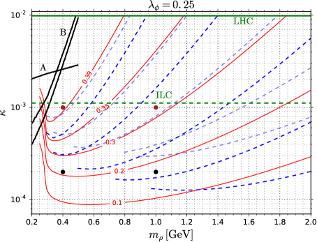
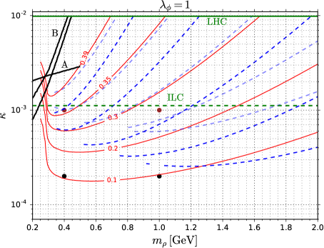
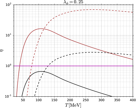
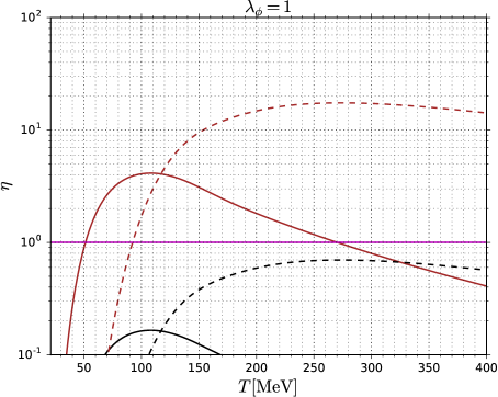
Figure 1: Top: contour lines of constant $\Delta N_{\rm eff}$ in ($m_{\rho}$, $\kappa$) plane for $\lambda_{\phi}=0.25$ (left panel) and $\lambda_{\phi}=1$ (right panel) obtained with eq. (48) in Maxwell-Boltzmann approximation (dark/light blue dashed lines include annihilation into muons and pions/muons only) and eq. (12) with full particles statistics (red lines – see details in sec. 4.2). Black lines correspond to astrophysical bounds [26]: for Goldstone boson free-streaming out of the proto-neutron stars (A) and for energy loss due to exotic species in SN 1987A in two different approximations (B). Green lines denote current (LHC – eq. (33)) and future (ILC for $B_{\rm inv}=0.3\%$) limit on invisible Higgs decay. We did not include effects from the CDM sector. Bottom: $\eta(T)$ dependence (see eq. (49)) for large dots marked in the upper panels – brown (black) lines correspond to $\kappa=10^{-3}\;(2\cdot 10^{-4})$, whereas solid (dashed) to $m_{\rho}=0.4\;(1)$ GeV. The freeze-out process for parameters corresponding to the black dots for $\kappa=2\cdot 10^{-4}$ is presented in more detail in Fig. 2.

$$\mathcal{C}\frac{x_{f}^{4}}{\sqrt{g_{*}(x_{f})}}{\rm K}_{1}\left(\frac{x_{f}\,m_{\rho}}{m_{\mu^{\pm}}}\right)=1\,,$$ (49)

where

$$\mathcal{C}\equiv\frac{\kappa^{2}}{\lambda_{\phi}}\frac{\sqrt{45}\,\zeta(3)}{32\pi^{5/2}}\frac{m_{\rho}^{5}M_{\rm Pl}}{m_{h}^{4}m_{\mu^{\pm}}^{2}}\left[\left(1-\frac{4m_{\mu^{\pm}}^{2}}{m_{\rho}^{2}}\right)^{3/2}+\frac{1}{27}\frac{m_{\rho}^{2}}{m_{\mu^{\pm}}^{2}}\left(1+\frac{11}{2}\frac{m_{\pi}^{2}}{m_{\rho}^{2}}\right)^{2}\left(1-\frac{4m_{\mu^{\pm}}^{2}}{m_{\rho}^{2}}\right)^{1/2}\right]\,.$$ (50)

In our numerical calculations we use the number of the effective degrees of freedom, $g_{*}(x)$, as given in [27]. In the upper panels of Fig. 1 we plotted $\Delta N_{\rm eff}$ obtained in the instantaneous freeze-out approximation, $Y=Y_{\rm eq}(x_{f})$, as a function of $m_{\rho}$ and $\kappa$ (blue lines), using definition (47) and the freeze-out temperature calculated from eq. (49). The results are compared to those obtained by solving the Boltzmann equation (red lines) – see sec. 4.2. In almost all cases the instantaneous freeze-out approximation overestimates $\Delta N_{\rm eff}$ for a given values of $\kappa$ and $\lambda_{\phi}$ (dark blue lines are below corresponding red lines). The best agreement between the instantaneous freeze-out approximation and the full result is achieved for $\Delta N_{\rm eff}$ close to 0.1, although in that region the instantaneous freeze-out approximation works only for $m_{\rho}\gtrsim 1$ GeV. Note also that neglecting the $\sigma$ annihilation into pions (given by eq. (40)), while keeping only annihilation into muons (39) (light blue lines in Fig. 1), leads to quite substantial underestimation of the resulting $\Delta N_{\rm eff}$ (the difference amplifies when $\kappa$ decreases).

It is worth emphasizing that the instantaneous freeze-out approximation breaks down for very small $\kappa$ and $m_{\rho}\lesssim 1$ GeV. Thus, exploration of this part of the parameter space requires a more accurate approach, which we will discuss in the next section. Let us only add that the above-mentioned problem is related to the stiffness of condition (48). As we can see in the lower panels of Fig. 1, for small enough $\kappa$ the $\eta(T)$ function never reaches 1.

The current experimental limits, shown in Fig. 1, exclude $\kappa\gtrsim 10^{-2}$ and the region of small $m_{\rho}$ with $\kappa\gtrsim 10^{-3}$. Note also that we conservatively do not consider here the CDM sector, which could (depending on the dark matter mass) constrain the parameter space even further [21], [26].

4.2 Solutions of the Boltzmann equation

In this subsection we compare the results obtained from solutions of the Boltzmann equation (with statistics of incoming and outgoing particles taken into account) with those obtained with the approximate methods introduced in subsection 2.1 (which include some effects of incoming particles statistics) and with the instantaneous freeze-out approximation discussed in the previous subsection.

Regions of small $\kappa$, where the last approximation breaks down, are especially important from the viewpoint of near future experiments that will be able to probe $\Delta N_{\rm eff}$ with accuracy even better than $0.03$. Let us start the discussion by considering two sample points from the parameter space with small $\kappa$: two lower (black) dots in the upper left panel of Fig. 1.

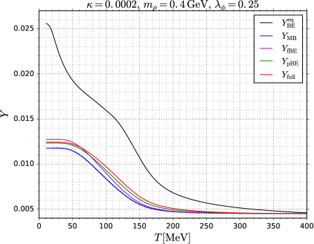
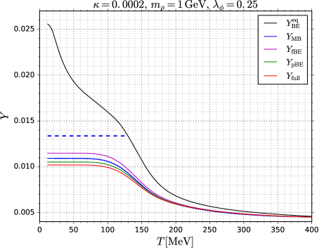
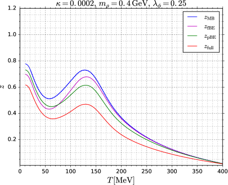
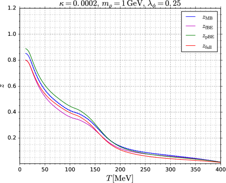
Figure 2: Yield $Y$ (upper panels) and pseudopotential $z$ (lower panels) of Goldstone boson $\sigma$ as functions of temperature for $\lambda_{\phi}=0.25$, $\kappa=2\cdot 10^{-4}$ and for two values of $m_{\rho}$ – see black dots in the upper left panel of Fig. 1. Line colors (corresponding to the methods used) are described in the legends. Dashed blue line in the upper right panel denotes the instantaneous freeze-out approximation result (see Fig. 1).

In Fig. 2 we show corresponding evolutions of $Y(T)$ and $z(T)$ for all three approximations described in section 2.1 as well as for the most accurate of our methods. Line colors i.e. blue, violet, green and red correspond to the pure MB approximation (point 1. under eq. (20)), fractional inclusion of incoming particles statistics (point 2. under eq. (20)), partial inclusion of incoming particles statistics (point 3. under eq. (21)) and full inclusion of particles statistics (eq. (12)), respectively. As we have already seen in Fig. 1, the instantaneous freeze-out approximation (dashed blue line in the upper right panel in Fig. 2) overestimates the relic density, as compared to the solutions of the Boltzmann equation (with full or any approximate inclusion of statistics effects). Such behavior is related to the convexity of $g_{*}(T)$ function, which for $T\sim 100\div 200$ MeV and $30\div 50$ MeV is characterized by strong variability. As a result, it is harder for $\sigma$ particles to follow the equilibrium density i.e. larger $\kappa$ is required as compared to the instantaneous freeze-out approximation, where the effect from $g_{*}(T)$ is point-wise. We checked that the instantaneous freeze-out approximation gives results closer to those obtained by integrating the Boltzmann equation when $g_{*}(T)$ during the $\sigma$ freeze-out changes relatively mildly (e.g. for $T\gtrsim 200$ MeV). However, the accuracy obtained with the instantaneous freeze-out approximation is typically worse than the accuracy of other approximate methods discussed in this work. One can also include the backreaction of $g_{\sigma}(x)$ on $g_{*}(x)$, however we checked numerically that this effect is negligible in the whole range of the analyzed parameter space.

It is also worth noting in the left panels of Fig. 2 that $\sigma$ freezes in for $T\sim 60\div 130$ MeV. For such temperatures the pseudopotential $z(T)$ decreases with time, which is related to the fact that the annihilation cross section for small $m_{\rho}$ reaches its maximum in this temperature range (see also $\eta(T)$ dependence in the lower panels of Fig. 1).

Having discussed general features of the lines presented in Fig. 2, let us now take a closer look at the differences between approximations in solving the Boltzmann equation, described in sec. 2.1. We checked both analytically and numerically that in the range of analyzed parameter space the phase space integral (41) may be expressed for different configurations of incoming/outgoing particles statistics as

$$\mathscr{D}\Phi_{\rm fBE} \approx\mathscr{D}\Phi_{\rm MB}\times\zeta^{\rm in}\,, \mathscr{D}\Phi_{\rm fFD} \approx\mathscr{D}\Phi_{\rm MB}\times\zeta^{\rm in}\,,$$ (51)

$$\mathscr{D}\Phi_{\rm pBE} \approx\mathscr{D}\Phi_{\rm MB}\times\frac{1}{\zeta^{\rm in}}\coth\left(\frac{m_{\rho}x}{4m_{\mu^{\pm}}}\right)\,, \mathscr{D}\Phi_{\rm pFD} \approx\mathscr{D}\Phi_{\rm MB}\times\frac{1}{\zeta^{\rm in}}\tanh\left(\frac{m_{\rho}x}{4m_{\mu^{\pm}}}\right)\,,$$ (52)

$$\mathscr{D}\Phi_{\rm BEFD} \approx\mathscr{D}\Phi_{\rm MB}\,, \mathscr{D}\Phi_{\rm FDBE} \approx\mathscr{D}\Phi_{\rm MB}\,,$$ (53)

$$\mathscr{D}\Phi_{\rm BEBE} \approx\mathscr{D}\Phi_{\rm MB}\times\coth^{2}\left(\frac{m_{\rho}x}{4m_{\mu^{\pm}}}\right)\,, \mathscr{D}\Phi_{\rm FDFD} \approx\mathscr{D}\Phi_{\rm MB}\times\tanh^{2}\left(\frac{m_{\rho}x}{4m_{\mu^{\pm}}}\right)\,,$$ (54)

where (see eq. (42))

$$\mathscr{D}\Phi_{\rm MB}=e^{-2z}\frac{\sum_{\rm spins}|M|^{2}}{2x}\sqrt{\frac{m_{\rho}^{2}}{m_{\mu^{\pm}}^{2}}-4}\;{\rm K}_{1}\left(\frac{x\,m_{\rho}}{m_{\mu^{\pm}}}\right)\,.$$ (55)

This clearly shows that for the cases when the incoming and outgoing particles have different statistics (BEFD or FDBE) the effects of statistics of initial and final states cancel each other to large extend and the MB approximation works quite well. When the initial and final particles have the same statistics one gets amplification (BEBE) or suppression (FDFD) with respect to the MB approximation. In Weinberg’s Higgs portal model one has to consider a combined case i.e. BEFD (annihilation into muons) and BEBE (annihilation into pions). The effect from the latter (factor $\coth^{2}\left(m_{\rho}x/4m_{\mu^{\pm}}\right)$) starts to be important for small $m_{\rho}$ and $x$ (larger $T$) and also for small $\kappa$. The dependence on $\kappa$ follows from the fact that $\sigma$ with smaller $\kappa$ decouples at higher temperature i.e. at smaller $x$. These effects can be seen in Fig. 3, where for small enough $m_{\rho}$ and $\kappa$ red curves are placed partially under the blue ones i.e. in order to get a given value of $\Delta N_{\rm eff}$ smaller $\kappa$ is needed when using the Boltzmann equation with full statistics effects as compared to the MB approximation.

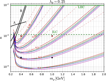
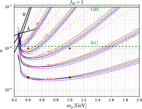
Figure 3: As top panels in Fig. 1 but for solutions of the Boltzmann equation with and without approximations defined in subsection 2.1. Colors for continuous lines are described in Fig. 2. Red dashed lines correspond to calculation with the pions contribution neglected.

One can also observe from Fig. 3 that for a given value of $\kappa$ and $m_{\rho}$ in most cases $\Delta N_{\rm eff}^{\rm pBE}<\Delta N_{\rm eff}^{\rm MB}<\Delta N_{\rm eff}^{\rm fBE}$ and relative differences between approximations decrease when $\kappa$ increases. Only for small enough $\kappa$ and $m_{\rho}$ we have $\Delta N_{\rm eff}^{\rm pBE}>\Delta N_{\rm eff}^{\rm MB}$. These relations can be easily understood with the help of eqs. (51) and (52). Moreover, for the most part of the parameter space (i.e. except the region with sufficiently small $m_{\rho}$ and $\kappa$, where pions statistics matters) full inclusion of incoming and outgoing statistics results in smaller $\Delta N_{\rm eff}$ than the above-mentioned approximations. There are two effects which explain this behavior. Firstly, from eq. (14) one can see that for given $z$ and $x$ inclusion of incoming particles statistics (here: BE) results in $n(x)$ (equivalently $Y(x)$) smaller than in the MB approximation (see eq. (17)) and the difference increases with $z$. Secondly, comparing eq. (12) and (18) one can show (see definition (8)) that for given $z$ and $x$ coefficients multiplying two terms in the RHS of eq. (12) ($J_{3}(z,x)/J_{2}(z,x)$ and $1/J_{2}(z,x)$ respectively) are smaller than those in eq. (18). First term in the RHS of eq. (12) dominates for small $z$ (when $Y(x)$ traces $Y_{\rm eq}(x)$) which causes weaker change in $|{\rm d}z/{\rm d}x|$ as compared to the MB case. When the second term starts to be important (for larger $z$) the coefficient $1/J_{2}(z,x)$ effectively weakens the annihilation strength (given by $\tilde{S}_{I}(z,x)$) leading to faster $|{\rm d}z/{\rm d}x|$ change with respect to other approximations. Both effects are visible in Fig. 2.

Contrary to naive expectations the MB approximation gives better accuracy than the fBE one, which includes the effect from incoming particles statistics only in $Y_{\rm eq}$. In order to obtain more precise results, it is necessary to take into account the effects from statistics also in the calculation of the thermal average of the appropriate cross section (pBE). Let us add that taking into account $\sigma$ annihilation into muons only (see Fig. 1 and Fig. 3) leads to sizable discrepancies with respect to the case when full annihilation is considered. The only exception holds for $m_{\rho}\leq 2m_{\pi}$ (i.e. when annihilation into pions does not take place) – one can observe that continuous lines rapidly change slope and red lines converge towards dashed ones.

Relative differences between our approximations may reach $\Delta N_{\rm eff}\sim 0.05$ and more. Thus, statistics of both incoming and outgoing particles are relevant, especially for moderate values of $\kappa$ and $m_{\rho}$. Minimal value of $\Delta N_{\rm eff}$ obtained in the scan ($\sim 0.06$) is related to the starting moment for the calculation i.e. $T_{\rm start}=400$ MeV, however for larger $T$ $Y_{\rm eq}(T)$ does not change significantly. Therefore, if $\sigma$ freezes out during or after the QCD phase transition, it shall give contribution to $N_{\rm eff}$ measurable by near future experiments. On the other hand, maximal $\Delta N_{\rm eff}$ equals approximately 0.5 and is achieved for large $\kappa$ and $m_{\rho}$ near the $h_{1}$ resonance (see eq. (37)), which is not preferred due to collider and astrophysical bounds. It is worth mentioning that the widely studied scenario with $\Delta N_{\rm eff}\sim 0.39$ for moderate values of $\lambda_{\phi}$ can be probed in major parts of the parameter space by the ILC (and new generation of CMB satellite experiments). However, the region with smaller $\lambda_{\phi}$ may be more challenging in this context as the lines of constant $\Delta N_{\rm eff}$ move towards smaller $\kappa$, becoming harder to be probed.

Let us finish this section with the discussion of differences between possible combinations of incoming and outgoing particles statistics (see eqs. (53) and (54)). In Fig. 4 we show similar plots to those presented in Fig. 3 but for $m_{\rho}\leq 1.2$ GeV, $\kappa\leq 10^{-3}$ and taking into account only (dominant) annihilation into pions (eq. (40)).

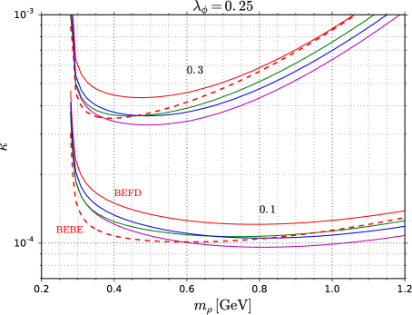
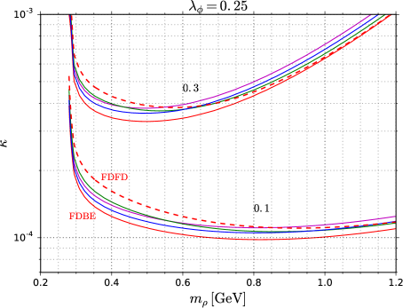
Figure 4: Contour lines of constant $\Delta N_{\rm eff}$ (top lines: 0.3, bottom lines: 0.1) in ($m_{\rho}$, $\kappa$) plane for $\lambda_{\phi}=0.25$ and bosons/fermions annihilation (left/right panel). Continuous (dashed) red lines correspond to mixed (homogeneous) statistics – see eqs. (53) and (54) e.g. BEBE case refers to $\sigma$ annihilation into pions in Weinberg’s Higgs portal model. Colors for other lines (MB, fBE/fFD, pBE/pFD) are the same as in the previous plots.

Then, BEBE case corresponds to Weinberg’s Higgs portal model with annihilation into muons neglected, while the others correspond to toy models with statistics of incoming and/or outgoing particles changed to the FD one. For mixed statistics BEFD/FDBE continuous red curves are placed above/below those that were obtained including the effects from incoming particles statistics only i.e. fBE/fBE and pBE/pFD (as well as from the MB approximation). For such mixed cases the effects of statistics of incoming and outgoing particles approximately cancel out in $\mathscr{D}\Phi$ (see eq. (53)). The main reason for smaller/bigger values of $\Delta N_{\rm eff}$ in such mixed cases, especially when compared to the results of the MB approximation, is the presence of the statistics factor $s_{\rm in}=\pm 1$ in eqs. (8) and (14) (as discussed below eq. (55)). As one can see (and what can be observed also in Fig. 4) for homogeneous statistics (BEBE and FDFD) the additional factors ($\coth^{2}\left(m_{\rho}x/4m_{\mu^{\pm}}\right)$ and $\tanh^{2}\left(m_{\rho}x/4m_{\mu^{\pm}}\right)$) in $\mathscr{D}\Phi$ given by (54)) are important for small exchanged particle mass (here $m_{\rho}$) and coupling (here $\kappa$). The effects of outgoing particle statistics decrease with $m_{\rho}$ and $\kappa$ and eventually become negligible.

5 Conclusions

We have investigated the problem of calculating the relic abundance of Dark Radiation which freezes out before the SM neutrinos decoupling. We used the Boltzmann equation for relativistic particles with their statistics taken into account. This method was compared to the instantaneous freeze-out approximation and to some approximate methods in which statistics of DR particles is included only in a limited way or completely ignored. As an interesting illustration of all these methods we analyzed in some detail the relic density of DR – measured by the change of the effective number of neutrino species $\Delta N_{\rm eff}$ – in the Weinberg’s Higgs portal model. The main results are as follows:

• The popular instantaneous freeze-out approximation can not be applied for small values of $m_{\rho}$ and $\kappa$ for which the Boltzmann equation must be used.

• In most of the remaining regions of the parameter space the instantaneous freeze-out approximation overestimates $\Delta N_{\rm eff}$. The main reason is convexity of $g_{*}(T)$ which in this simple method is not taken into account. The instantaneous freeze-out approximation gives best results for $\Delta N_{\rm eff}\sim 0.1$ and $m_{\rho}\gtrsim 1$ GeV. The resonant exchange of the scalar $\rho$ (for $m_{\rho}$ up to a few hundreds MeV) also plays an important role.

• When calculating the annihilation cross section of DR particles (Goldstone bosons $\sigma$) it is crucial to include muons and pions as the final states. Pions are quite often ignored which may lead to underestimation of $\Delta N_{\rm eff}$ by as much as 0.1.

• Not taking (fully) into account the statistics of DR particles and particles into which DR annihilates may change the obtained values of $\Delta N_{\rm eff}$ by up to about 0.05. Contrary to naive expectation, in some parts of the parameter space ignoring the effects of statistics (MB approximation) may give better prediction for $\Delta N_{\rm eff}$ than inclusion of only some of the effects – those in evaluation of $Y_{\rm eq}(T)$ – due to the DR statistics (fBE approximation). Inclusion of more effects from the DR statistics (pBE approximation) leads to more accurate results than those obtained using the simplest MB approximation.

The present experimental data leave quite substantial uncertainty in determining the value of $\Delta N_{\rm eff}$. One may expect that results of near future experiments will lead to much better determination of $\Delta N_{\rm eff}$ and will allow to test scenario considered in this work. In such a case it will be important not only to use the statistics of incoming and outgoing particles in the appropriate Boltzmann equation but maybe also to take into account the effects of deviations from kinetic equilibrium. This may be especially important for cases with resonant exchange of $\rho$ when DR particles $\sigma$ may decouple kinetically before thermal decoupling. This might happen because in elastic scattering particle $\rho$ is exchanged in the t channel for which there is no resonant enhancement [28]. Another potentially important issue is the relation between the DR and CDM sectors. We assumed in our analysis that CDM particles are so heavy that they do not influence the DR properties. However, it may occur, especially when future more precise experimental results are available, that the case of lighter CDM should be considered simultaneously with DR.

References

- [1] P. A. R. Ade et al. [Planck Collaboration], Astron. Astrophys. 594 (2016) A13 [arXiv:1502.01589 [astro-ph.CO]].
- [2] A. G. Riess et al., Astrophys. J. 826 (2016) no.1, 56 [arXiv:1604.01424 [astro-ph.CO]].
- [3] R. C. Nunes and A. Bonilla, Mon. Not. Roy. Astron. Soc. 473 (2018) 4404 [arXiv:1710.10264 [astro-ph.CO]].
- [4] A. Heavens, Y. Fantaye, E. Sellentin, H. Eggers, Z. Hosenie, S. Kroon and A. Mootoovaloo, Phys. Rev. Lett. 119 (2017) no.10, 101301 [arXiv:1704.03467 [astro-ph.CO]].
- [5] K. N. Abazajian et al. [CMB-S4 Collaboration], arXiv:1610.02743 [astro-ph.CO].
- [6] S. Weinberg, Phys. Rev. Lett. 110 (2013) no.24, 241301 [arXiv:1305.1971 [astro-ph.CO]].
- [7] S. Hannestad and J. Madsen, Phys. Rev. D 52 (1995) 1764 [astro-ph/9506015].
- [8] A. D. Dolgov, S. H. Hansen and D. V. Semikoz, Nucl. Phys. B 503 (1997) 426 [hep-ph/9703315].
- [9] N. Y. Gnedin and O. Y. Gnedin, Astrophys. J. 509 (1998) 11 [astro-ph/9712199].
- [10] G. Mangano, G. Miele, S. Pastor, T. Pinto, O. Pisanti and P. D. Serpico, Nucl. Phys. B 729 (2005) 221 [hep-ph/0506164].
- [11] S. Esposito, G. Miele, S. Pastor, M. Peloso and O. Pisanti, Nucl. Phys. B 590 (2000) 539 [astro-ph/0005573].
- [12] G. Mangano, G. Miele, S. Pastor and M. Peloso, Phys. Lett. B 534 (2002) 8 [astro-ph/0111408].
- [13] J. Birrell, J. Wilkening and J. Rafelski, J. Comput. Phys. 281 (2014) 896 [arXiv:1403.2019 [math.NA]].
- [14] J. Birrell, C. T. Yang, P. Chen and J. Rafelski, Phys. Rev. D 89 (2014) 023008 [arXiv:1212.6943 [astro-ph.CO]].
- [15] A. D. Dolgov and K. Kainulainen, Nucl. Phys. B 402 (1993) 349 [hep-ph/9211231].
- [16] J. Bernstein, L. S. Brown and G. Feinberg, Phys. Rev. D 32 (1985) 3261.
- [17] P. Gondolo and G. Gelmini, Nucl. Phys. B 360 (1991) 145.
- [18] C. Garcia-Cely, A. Ibarra and E. Molinaro, JCAP 1311 (2013) 061 [arXiv:1310.6256 [hep-ph]].
- [19] V. Khachatryan et al. [CMS Collaboration], JHEP 1702 (2017) 135 [arXiv:1610.09218 [hep-ex]].
- [20] W. F. Chang and J. N. Ng, JCAP 1607 (2016) no.07, 027 [arXiv:1604.02017 [hep-ph]].
- [21] L. A. Anchordoqui, P. B. Denton, H. Goldberg, T. C. Paul, L. H. M. Da Silva, B. J. Vlcek and T. J. Weiler, Phys. Rev. D 89 (2014) no.8, 083513 [arXiv:1312.2547 [hep-ph]].
- [22] M. B. Voloshin, Sov. J. Nucl. Phys. 44 (1986) 478 [Yad. Fiz. 44 (1986) 738].
- [23] J. F. Gunion, H. E. Haber, G. L. Kane and S. Dawson, Front. Phys. 80 (2000) 1.
- [24] K. W. Ng, H. Tu and T. C. Yuan, JCAP 1409 (2014) no.09, 035 [arXiv:1406.1993 [hep-ph]].
- [25] G. Mangano, G. Miele, S. Pastor and M. Peloso, Phys. Lett. B 534 (2002) 8 [astro-ph/0111408].
- [26] H. Tu and K. W. Ng, JHEP 1707 (2017) 108 [arXiv:1706.08340 [hep-ph]].
- [27] M. Drees, F. Hajkarim and E. R. Schmitz, JCAP 1506 (2015) no.06, 025 [arXiv:1503.03513 [hep-ph]].
- [28] T. Binder, T. Bringmann, M. Gustafsson and A. Hryczuk, Phys. Rev. D 96 (2017) no.11, 115010 [arXiv:1706.07433 [astro-ph.CO]].