Transition to high-dimensional chaos in nonsmooth dynamical systems

Abstract

We uncover a route from low-dimensional to high-dimensional chaos in nonsmooth dynamical systems as a bifurcation parameter is continuously varied. The striking feature is the existence of a finite parameter interval of periodic attractors in between the regimes of low- and high-dimensional chaos. That is, the emergence of high-dimensional chaos is preceded by the system’s settling into a totally nonchaotic regime. This is characteristically distinct from the situation in smooth dynamical systems where high-dimensional chaos emerges directly and smoothly from low-dimensional chaos. We carry out an analysis to elucidate the underlying mechanism for the abrupt emergence and disappearance of the periodic attractors and provide strong numerical support for the typicality of the transition route in the pertinent two-dimensional parameter space. The finding has implications to applications where high-dimensional and robust chaos is desired.

I Introduction

In nonlinear dynamical systems, there are two kinds of chaos: low-dimensional and high-dimensional. The characteristic feature of a low-dimensional chaotic invariant set (e.g., an attractor) is that it has only one positive Lyapunov exponent, examples of which include the classic Lorenz Lorenz:1963 and Rössler Rossler:1976 attractors. High-dimensional chaotic sets are those that possess more than one positive Lyapunov exponent IM:1987 ; BHGY:1997 ; MM:2009 ; IMAD:2015 . The difference between low- and high-dimensional chaos can be appreciated in terms of significant issues such as control. The well established Ott-Grebogi-Yorke paradigm OGY:1990 ; BGLMM:2000 of controlling chaos is most effective for low-dimensional chaotic systems, and controlling high-dimensional chaos AGOY:1992 ; GL:1997 ; BGLMM:2000 has remained to be a challenging problem.

In nonlinear dynamics, the four routes to chaos, namely, period-doubling Feigenbaum:1978 , intermittency PM:1980 , crisis GOY:1983 , and quasiperiodicity RT:1971 ; GS:1975 ; NRT:1978 , concerned about the bifurcation to a low-dimensional chaotic attractor. There was also work on the transition from low- to high-dimensional chaos HL:1999 ; HL:2000 ; DL:2000 ; PSM:2001 ; PM:2005 in smooth dynamical systems. A general phenomenon is that the second Lyapunov exponent passes through zero and becomes positive smoothly as a parameter changes through the transition point. Heuristically, this can be understood in light of transition to chaos in random dynamical systems YOC:1990 ; RHKK:2000 ; LLBS:2002 ; LLBS:2003 ; XLZD:2003 , in systems with a symmetry Lai:1996a , and in quasiperiodically driven systems Lai:1996b ; LFG:1996 ; YL:1996 . In particular, before the transition, the system is already chaotic with one positive Lyapunov exponent - the largest exponent giving the exponential growth of an infinitesimal vector in the corresponding tangent subspace. For convenience, we call it the primary tangent subspace. The evolution of the vector in the secondary tangent subspace corresponding to the second nontrivial Lyapunov exponent can then be regarded as being subject to an indirect, chaotic or effectively “random” driving from the dynamics in the primary tangent subspace. Under such a driving, an infinitesimal vector in the secondary tangent subspace will exhibit temporal episodes of “expansion” or “contraction,” a generic feature in random dynamical systems YOC:1990 . The second nontrivial Lyapunov exponent will then exhibit fluctuations in finite time between positive and negative values. The asymptotic value of the exponent depends on the relative weights of the underlying infinitesimal tangent vector in the expanding or contracting phase HL:1999 : the value is negative if the contraction phase over weighs the expansion phase, and vice versa for a positive value. Transition to high-dimensional chaos occurs when the contraction and expansion weights are balanced. Since the weights vary smoothly with the bifurcation parameter HL:1999 , the second nontrivial Lyapunov exponent passes through zero smoothly. The generic feature associated with the transition in smooth dynamical systems is thus that high-dimensional chaos arises directly and smoothly from low-dimensional chaos HL:1999 ; HL:2000 ; DL:2000 .

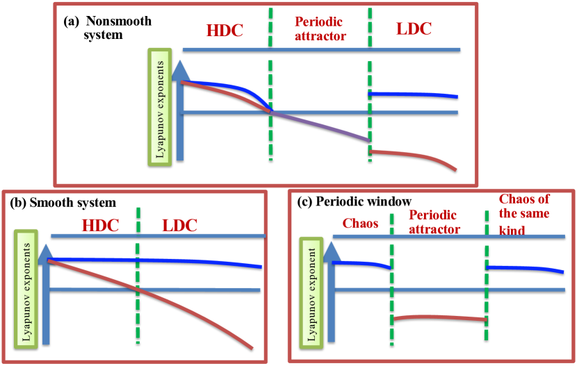
Figure 1: Schematic illustration of transition scenarios to high-dimensional chaos (HDC) in nonsmooth and smooth dynamical systems. (a) The main result of the paper. As a parameter (e.g., the coupling strength) is reduced from the regime of low-dimensional chaos (LDC) with a single positive Lyapunov exponent, an open parameter interval of periodic attractors arises before HDC emerges. This transition scenario should be contrasted to that in smooth dynamical systems in (b) and is also fundamentally different from the dynamical behavior before and after the occurrence of a periodic window in (c). (b) Transition to HDC in smooth dynamical systems where the second largest Lyapunov exponent passes through zero smoothly at the transition point. That is, HDC emerges exactly where LDC ends. (c) The behavior about a periodic window, where chaos on both sides of the window is of the same kind: either low-dimensional or high-dimensional.

In this paper, we investigate the transition to high-dimensional chaos in nonsmooth dynamical systems that arise commonly in physical, engineering, and biological applications such as impact oscillators TG:1983 ; SH:1983 ; Whiston:1983 ; Nordmark:1991 ; CONG:1994 ; CCGO:1996 , electronic circuits BYG:1998 ; BG:1999 ; BRG:2000 , and neuronal networks NC:2016 ; NTS:2016 . Mathematically, a typical representation of such systems is piecewise smooth systems, e.g., a one-dimensional piecewise smooth map that can generate low-dimensional chaos. For a system with two pieces, the phase space can be divided into two regions where the dynamical equations in each region are different but are nevertheless smooth, with a border separating the two regions. This setting is representative of physical systems such as electronic switching circuits BYG:1998 ; BG:1999 ; BRG:2000 . Previous mathematical analyses of piecewise smooth systems with low-dimensional chaos revealed interesting phenomena such as period-adding bifurcations and transition to chaos from a periodic attractor of arbitrary period, as a result of “border collision” in phase space NY:1992 ; NOY:1994 ; DNOYY:1999 ; LZCY:2002 ; HAN:2004 ; GB:2005 ; ASB:2007 ; DL:2008 . Because our goal is to uncover and understand how high-dimensional chaos may arise from low-dimensional chaos in nonsmooth systems, we consider the minimal setting of two coupled piecewise smooth subsystems, each capable of exhibiting low-dimensional chaos. At zero coupling, the two subsystems are isolated and the system as a whole has two positive Lyapunov exponents - a trivial type of high-dimensional chaos. In the weak coupling regime, there is interaction between the two subsystems and the system possesses high-dimensional chaos. In the strong coupling regime, synchronization between the two subsystems can occur, and the dynamics of the full system are effectively those of a single subsystem. As a result, the system exhibits low-dimensional chaos. In the intermediate coupling regime, a transition between low- and high-dimensional chaos can be expected. Is the transition scenario any different than that in smooth dynamical systems?

The main finding of this paper is that, in nonsmooth dynamical systems, there can be two distinct routes to high-dimensional chaos: one that is similar to and another characteristically different from that in smooth dynamical systems. In particular, depending on the system parameter values, high-dimensional chaos can arise directly and smoothly from low-dimensional chaos, as in smooth dynamical systems. The striking phenomenon is the existence of an open parameter region in nonsmooth systems where a nonchaotic, “buffer” regime with a periodic attractor arises in between regions of low- and high-dimensional chaos. For example, for the minimal coupled nonsmooth system, as the coupling parameter is decreased from the low-dimensional, synchronous chaos regime, a periodic attractor can arise abruptly and last for a finite parameter interval. At a smaller parameter value, a high-dimensional chaotic attractor emerges abruptly from the periodic attractor. The “buffer” periodic attractor occurs in an open interval of the coupling parameter. In a two-dimensional parameter space, the buffer or “precursor” periodic attractor occupies a finite region - a “bubble,” signifying its typicality. The emergence of the bubble region can generally be attributed to border collision bifurcations, for which we provide a detailed analysis. The same transition scenario can occur when the phase space dimension is much larger than two, e.g., in a system of a large number of coupled nonsmooth maps. In such a case, high-dimensional chaos manifests itself as synchronous clusters with distinct chaotic behaviors, low-dimensional chaos corresponds to globally synchronous chaos, and periodic synchronization occurs in the bubble region. A schematic illustration of our main result and its characteristic difference from the transition scenario in smooth dynamical systems as well as from that around a periodic window is presented in Fig. 1.

II Model and results

II.1 A system of coupled piecewise linear maps and Lyapunov exponents

A typical class of nonsmooth dynamical systems is piecewise smooth maps CHHBKM:1992 ; QWH:1998 ; WDHWMH:2001 ; LHJ:2005 ; YWQ:2015 . To investigate the transition route to high-dimensional chaos, we use coupled map lattices Kaneko:1989 ; Kaneko:1990a ; Kaneko:1990b ; PPM:2001 ; PMM:2001 ; PMM:2002 ; TKWTBT:2008 ; PBH:2009 ; PR:2015 ; Kaneko:2015 . Specifically, we consider the following system of $N$ globally coupled, piecewise smooth maps:

$$x_{n+1}(i)=(1-\varepsilon)f[x_{n}(i)]+\frac{\varepsilon}{N}\sum_{j=1}^{N}f[x_{n}(j)],$$ (1)

where $x_{n}(i)$ is the dynamical variable of the $i$th node at time $n$, $\varepsilon\in[0,1]$ is a coupling parameter, and $f(x)$ represents the nodal dynamics. To be concrete, we consider the following one-dimensional piecewise linear map

$$f(x)=\left\{\begin{array}[]{ll}\alpha x-\mu,&\leavevmode\nobreak\ x<0,\\ \beta x-\mu-\gamma,\nobreak\leavevmode&\leavevmode\nobreak\ x>0,\end{array}\right.$$ (2)

where $\alpha,\beta,\mu$ and $\gamma$ are parameters. There is a nonsmooth border at $x=0$ where the left and right limits of the mapping function are not identical. To investigate the transition to high-dimensional chaos, we require that the isolated nodal dynamics generate a low-dimensional chaotic attractor, which can be realized for, e.g., the following parameter setting: $\alpha=0.4,\beta=-8,\mu=0.1$, and $\gamma=0$. The Lyapunov exponent of this attractor is $\lambda_{0}\approx 0.251$.

A typical dynamical state of system (1) is cluster formation, where the dynamics of all nodes within a cluster are synchronized but those among different clusters are unsynchronized. For simplicity, we consider the case of a two-cluster state PBH:2009 :

$$\begin{array}[]{ll}x_{n}(1)=x_{n}(2)=\cdot\cdot\cdot=x_{n}(N_{1})=x_{n},\\ x_{n}(N_{1}+1)=x_{n}(N_{1}+2)=\cdot\cdot\cdot=x_{n}(N)=y_{n},\end{array}$$ (3)

where $N_{1}$ and $N_{2}=N-N_{1}$ are the numbers of nodes in the two clusters. Because of synchronization within each cluster, we obtain an effective two-dimensional nonsmooth map:

$$x_{n+1} = [1-\varepsilon(1-r))f(x_{n})+\varepsilon(1-r)f(y_{n}),$$ (4)

$$y_{n+1} = \varepsilon rf(x_{n})+(1-\varepsilon r)f(y_{n}),$$

where $r=N_{1}/N$ is the fraction of nodes belonging to the $x$ cluster. In the thermodynamic limit $N\to\infty$, $r$ is a continuous parameter. System (4) describes the dynamical evolution of the two cluster state in system (1). For $r=1/2$, the two clusters are symmetric with respect to each other PBH:2009 . As we will demonstrate, the two distinct routes to high-dimensional chaos occur in different intervals of $r$ values.

Because of the mirror symmetry with respect to $r=1/2$, we introduce the parameter $\bar{r}=r-1/2$ to rewrite Eq. (4) as

$$\begin{array}[]{ll}x_{n+1}=(1-\varepsilon(\frac{1}{2}-\bar{r}))x_{n}+\varepsilon(\frac{1}{2}-\bar{r})y_{n},\\ y_{n+1}=\varepsilon(\frac{1}{2}+\bar{r})x_{n}+(1-\varepsilon(\frac{1}{2}+\bar{r}))y_{n},\end{array}$$ (5)

which has an exact synchronous solution: $x_{n}=y_{n}=s_{n}$. We write ${\bf x}_{n+1}={\bf F}({\bf x}_{n})$, where ${\bf x}\equiv(x,y)^{T}$ and the symbol “$T$” denotes transpose. The corresponding variational equations are

$$\!\left(\!\!\begin{array}[]{l}\!\delta x_{n+1}\\ \!\delta y_{n+1}\\ \end{array}\!\!\!\!\right)\!\!=\!\!f^{\prime}\!(\!s_{n}\!)\!\!\left(\!\!\!\begin{array}[]{cc}1-\varepsilon(\frac{1}{2}-\bar{r})&\varepsilon(\frac{1}{2}-\bar{r})\\ \varepsilon(\frac{1}{2}+\bar{r})&1-\varepsilon(\frac{1}{2}+\bar{r})\\ \end{array}\!\!\!\right)\!\!\!\left(\!\!\begin{array}[]{l}\!\delta x_{n}\\ \!\delta y_{n}\\ \end{array}\!\!\!\right),$$ (6)

where $\delta x_{n}=x_{n}-s_{n}$, $\delta y_{n}=y_{n}-s_{n}$, and $f^{\prime}(s_{n})$ is the derivative of the map function evaluated at the synchronization manifold. The two eigenvalues of the coupling matrix are $u_{1}=1$ and $u_{2}=1-\varepsilon$. The corresponding transform matrix is given by

$$\mathbf{Q}=\left(\begin{array}[]{cc}1&\frac{\bar{r}-\frac{1}{2}}{\frac{1}{2}+\bar{r}}\\ 1&1\\ \end{array}\right).$$ (7)

The transform $(\delta\tilde{x}_{n},\delta\tilde{y}_{n})^{T}=\mathbf{Q}^{-1}\cdot(\delta x_{n},\delta y_{n})^{T}$ leads to a diagonally decoupled form of Eq. (6):

$$\left(\!\begin{array}[]{c}\delta\tilde{x}_{n+1}\\ \delta\tilde{y}_{n+1}\\ \end{array}\!\right)=f^{\prime}(s_{n})\!\!\left(\!\begin{array}[]{cc}1&0\\ 0&1-\varepsilon\\ \end{array}\!\right)\!\!\!\left(\!\begin{array}[]{c}\delta\tilde{x}_{n}\\ \delta\tilde{y}_{n}\\ \end{array}\!\right)$$ (8)

The transverse Lyapunov exponent is given by

$$\lambda_{\perp}=\ln(1-\varepsilon)+\lambda_{0}$$ (9)

where $\lambda_{0}>0$ is the Lyapunov exponent of the chaotic attractor of the individual map. Stable synchronization can be achieved for $\lambda_{\perp}<0$. The critical value of the coupling parameter above which synchronization occurs is $\varepsilon_{c}=1-e^{-\lambda_{0}}\approx 0.222$.

The Lyapunov exponents of the asymptotic invariant set of the system can be calculated from the Jacobian matrix $\mathbf{DF}$ associated with a typical trajectory $\{(x_{n},y_{n})\}_{n=0}^{\infty}$:

$$\mathbf{DF}^{n}(x_{0},y_{0})=\prod_{j=0}^{n-1}\mathbf{DF}(x_{j},y_{j}).$$ (10)

The eigenvalues of the Jacobian matrix are given by

$$\mathrm{det}(\mathbf{DF}^{n}-u\mathbf{I})=0.$$ (11)

We have that the eigenvalue $u$ satisfies

$$u^{2}-\tau u+\Delta=0,$$ (12)

where $\tau\equiv\mathrm{trace}(\mathbf{DF}^{n})$ and $\Delta\equiv\det(\mathbf{DF}^{n})$. For $\tau^{2}-4\Delta\geq 0$, the eigenvalues are real and the Lyapunov exponents are given by

$$\lambda_{1}=\frac{1}{n}\ln|u_{1}|,\leavevmode\nobreak\ \ \lambda_{2}=\frac{1}{n}\ln|u_{2}|,$$ (13)

where $u_{1}=(\tau+\sqrt{\tau^{2}-4\Delta})/2$ and $u_{2}=(\tau-\sqrt{\tau^{2}-4\Delta})/2$. For $\tau^{2}-4\Delta<0$, we obtain a pair of complex conjugate eigenvalues. In this case, the Lyapunov exponents are determined by the absolute value of the eigenvalues $|u|$. We have

$$\lambda_{1,2}=\frac{1}{n}\ln|\mathrm{Re}(u)|.$$ (14)

where $\mathrm{Re}(u)=\Delta$. For a periodic attractor of period-m, we have $n=m$.

II.2 Main result: coexistence of distinct transition routes to high-dimensional chaos

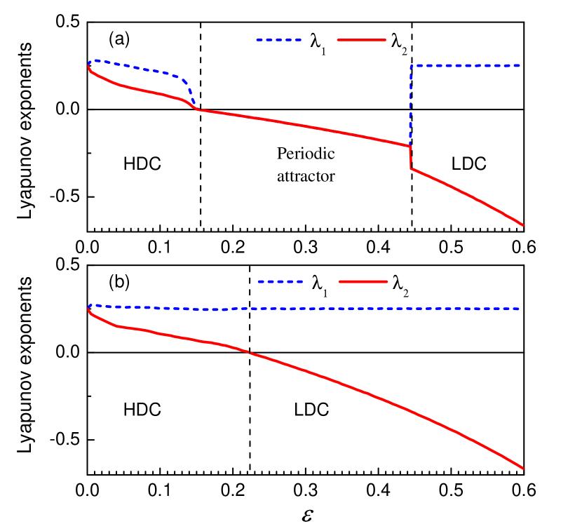
Figure 2: (Color online) Two distinct routes of transition to high-dimensional chaos in nonsmooth dynamical systems. (a) For $\bar{r}=0.3$, the transition route follows the scenario in Fig. 1(a). As the coupling parameter $\varepsilon$ is decreased from a relatively large value where there is synchronous chaos with one positive Lyapunov exponent (LDC), a periodic attractor arises. A high-dimensional chaotic attractor with two positive Lyapunov exponents (HDC) emerges when the periodic attractor disappears. (b) For $\bar{r}=0.48$, HDC arises directly and smoothly from LDC as in smooth dynamical systems.

For system (5), we uncover a distinct route from low-dimensional to high-dimensional chaos as the coupling parameter $\varepsilon$ is reduced. In particular, for relatively large values of $\varepsilon$, there is synchronous chaos and the system has a low-dimensional chaotic attractor with one positive Lyapunov exponent. As $\varepsilon$ is decreased, a periodic attractor with two identical negative Lyapunov exponents arises abruptly and lasts for a finite parameter interval. High-dimensional chaos with two positive Lyapunov exponents emerges where the periodic attractor disappears. That is, there exists a “buffer” region of some periodic attractor in between low- and high-dimensional chaos. This transition scenario to high-dimensional chaos, as exemplified by Fig. 2(a) [schematically illustrated in Fig. 1(a)] for $\bar{r}=0.3$, is unique for nonsmooth dynamical systems. For a different value of parameter $\bar{r}$, the typical route to high-dimensional chaos in smooth dynamical systems [schematically illustrated in Fig. 1(b)] occurs, where a high-dimensional chaotic attractor emerges directly and smoothly from a low-dimensional chaotic attractor, as demonstrated in Fig. 2(b) for $\bar{r}=0.48$. Nonsmooth dynamical systems thus exhibit richer transition scenarios to high-dimensional chaos than smooth systems.

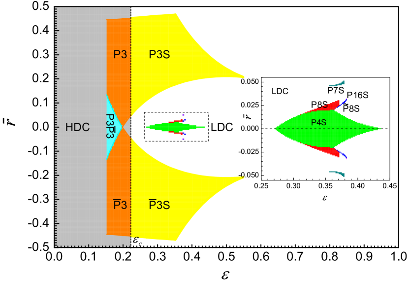
Figure 3: (Color online) Phase diagram of distinct attractors in the parameter plane ($\varepsilon$, $\bar{r}$). There is a mirror symmetry with respect to $\bar{r}=0$. A period-m attractor is denoted as Pm. The vertical dashed line represents the critical value $\varepsilon_{c}$ of the coupling parameter beyond which synchronous chaos arises. Legends are: HDC - high-dimensional chaos, LDC - low-dimensional chaos (fully synchronous chaotic state - the blank region), P3 - clockwise period-3 attractor, $\mathrm{\bar{P}}$3 - counterclockwise period-3 attractor. Additional legends are: P3$\mathrm{\bar{P}}$3 - coexistence of two distinct period-3 attractors; P3S: coexistence of a clockwise period-3 attractor with LDC; $\mathrm{\bar{P}}$3S: counterclockwise period-3 attractor coexisting with LDC. Inset is magnification of the region enclosed by the dashed rectangular box in which periodic attractors of high periods (e.g., P8 and $\mathrm{\tilde{P}}$8) coexist with LDC.

To obtain a complete picture of the asymptotic attractors in different parameter regions, we calculate the phase diagram in the parameter plane $(\varepsilon,\bar{r})$, as shown in Fig. 3. The phase diagram has a mirror symmetry about $\bar{r}=0$. For example, the parameter regions in which two distinct period-3 attractors, P3 and $\mathrm{\bar{P}}$3, occur are symmetric about $\bar{r}=0$. In the strongly coupling regime, synchronous chaotic attractors arise: the system exhibits low-dimensional chaos, whereas high-dimensional chaos occurs in the weakly coupling regime. For $-0.45\lesssim\bar{r}\lesssim 0.45$, the transition from low- to high-dimensional chaos as the coupling parameter $\varepsilon$ is decreased follows the route as demonstrated schematically in Fig. 1(a) and realistically in Fig. 2(a), where the period-3 attractor occupies a large region in the parameter plane. For $0.45\lesssim|\bar{r}|<0.5$, the transition from low- to high-dimensional chaos follows the conventional route [Figs. 1(b) and 2(b)] as in smooth dynamical systems. There are also regions in the parameter plane where periodic attractors of various periods arise. For example, the region marked by P3$\mathrm{\bar{P}}$3 is one in which two symmetric period-3 attractors coexist, each with a distinct basin of attraction. There are also periodic attractors as a result of period-doubling bifurcations, such as those denoted as P4, P8, and P16, as well as those created by period-adding bifurcations, e.g., P3, P4, and P7. In the following, we carry out an analysis to elucidate the underlying mechanism for the abrupt emergence of the periodic attractors in between regimes of low- and high-dimensional chaos.

III Emergence of periodic attractors between regimes of low- and high-dimensional chaos

For nonsmooth dynamical system, linear stability analysis alone is often inadequate to characterize the bifurcations or transitions PBH:2009 . We find that, in our piecewise linear systems, the transition from low-dimensional chaos to a periodic attractor is typically of the second order, continuous type. The dynamical origin of the transition is border collision bifurcations.

III.1 Emergence of period-3 attractors

The period-3 attractors take up a considerable region in the two-dimensional parameter space. In order to determine the stability condition of the attractor, we examine its orbital structure as a bifurcation parameter is continuously varied. Taking advantage of the symmetry of the system, we focus on the region of $\bar{r}\geq 0$. The three orbital points are denoted as $(x_{1}^{*},y_{1}^{*})$, $(x_{2}^{*},y_{2}^{*})$ and $(x_{3}^{*},y_{3}^{*})$, where the first point $(x_{1}^{*},y_{1}^{*})$ is located at the bottom of the phase portrait: $y_{1}^{*}$ is the minimal value, as shown in Fig. 4. For $\bar{r}=0.3$, from Figs. 4(a,b), we see that, at the left boundary the stable period-3 attractor disappears without collision, while at the right boundary it disappears because of the collision between the $y_{2}$ orbit and the border $y=0$. The phase space for $\varepsilon=0.3$ is shown in Figs. 4(c,d), where the $x_{1}$ orbit collides with the border $x=0$ for a small value of $\bar{r}$ and the stable period-3 attractor disappears without collision for a large value of $\bar{r}$. For $\varepsilon=0.45$, as shown in Figs. 4(e,f), we see that the two boundaries of the disappearance of the period-3 attractor are both due to border collision bifurcations. In particular, the $x_{1}$ orbit collides with the border $x=0$ for a small value of $\bar{r}$ and the $y_{2}$ orbit collides with the border $y=0$ for a large value of $\bar{r}$.

Figure 4: (Color online) Emergence and disappearance of a period-3 attractor. The three orbital points are denoted by $(x_{1}^{*},y_{1}^{*})$, $(x_{2}^{*},y_{2}^{*})$ and $(x_{3}^{*},y_{3}^{*})$. Shown are examples of how the orbital points of the period-3 attractor depend on the bifurcation parameter $\varepsilon$ or $\bar{r}$: (a,b) $\bar{r}=0.3$, (c,d) $\varepsilon=0.3$, and (e,f) $\varepsilon=0.4$.

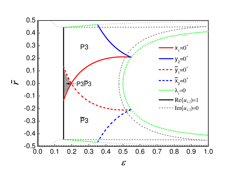
Figure 5: (Color online) Analysis of the period-3 attractor. The blue and red curves represent border collision bifurcations. The green dotted curves represent the critical condition for the largest Lyapunov exponent $\lambda_{1}$. The black line denotes the critical condition of the real part of complex conjugate eigenvalues. The dash lines indicate zero imaginary part of the complex conjugate eigenvalues.

Our detailed calculation reveals that there are two types of border collision bifurcations with the critical conditions given by

$$A:\left\{\begin{array}[]{c}(x_{2}^{*},y_{2}^{*})=\mathbf{F}^{3}[(x_{2}^{*},y_{2}^{*})],\\ y_{2}^{*}=0^{+},\\ \end{array}\right.$$ (15)

$$B:\left\{\begin{array}[]{c}(x_{1}^{*},y_{1}^{*})=\mathbf{F}^{3}[(x_{1}^{*},y_{1}^{*})],\\ x_{1}^{*}=0^{+},\end{array}\right.$$ (16)

where the superscript “+” denotes the situation where the orbital point collides with the discontinuous border from the positive side. The stability condition of the period-3 attractor can then be obtained. In particular, from Fig. 4, we have that the orbital points of the attractor satisfy the conditions $(x_{1}^{*}>0,y_{1}^{*}<0)$, $(x_{2}^{*}<0,y_{2}^{*}>0)$ and $(x_{3}^{*}>0,y_{3}^{*}>0)$. The Jacobian matrix evaluated at the attractor is

$$\mathbf{DF}^{3}=\mathbf{G}\!\left(\!\!\begin{array}[]{cc}\alpha&0\\ 0&\alpha\\ \end{array}\!\!\right)\!\mathbf{G}\!\left(\!\!\begin{array}[]{cc}\beta&0\\ 0&\alpha\\ \end{array}\!\!\right)\!\mathbf{G}\!\left(\!\!\begin{array}[]{cc}\alpha&0\\ 0&\beta\\ \end{array}\!\!\right),$$ (17)

with $\mathbf{G}$ being the coupling matrix

$$\left(\begin{array}[]{cc}\!1-\varepsilon(\frac{1}{2}-\bar{r})&\varepsilon(\frac{1}{2}-\bar{r})\\ \varepsilon(\frac{1}{2}+\bar{r})&1-\varepsilon(\frac{1}{2}+\bar{r})\\ \end{array}\!\right).$$ (18)

From the characteristic equation Eq. (17), we get

$$\Delta = (1-\varepsilon)^{3}\alpha^{4}\beta^{2},$$ (19)

$$\tau = \frac{1}{4}\alpha(\varepsilon-2)[((4\bar{r}^{2}-1)(\alpha-\beta)^{2}-4\alpha\beta)\varepsilon^{2}$$

$$- 4\alpha\beta(\varepsilon+1)].$$

Combining Eqs. (13)-(16) and (19) leads to the critical conditions for the period-3 attractor to be stable.

Figure 5 shows the results from the stability analysis. The stable period-3 attractor exists in the region surrounded by the curves of stability (denoted by the green dotted curves and the black line) and border collision bifurcations (denoted by red and blue curves). Comparing Fig. 5 with Fig. 3, we find a good agreement between the theoretical analysis and the numerically calculated structure of the parameter space for the period-3 attractor. Specifically, for a fixed value of $\bar{r}$, as the coupling parameter $\varepsilon$ is increased, the period-3 attractor undergoes a border collision bifurcation before it becomes unstable, corresponding to the the sudden transition from low-dimensional chaos to a periodic attractor, as shown in Fig. 2. In addition, there is a region surrounded by $x_{1}$, $\bar{y}_{1}$ and the stability curve, as marked by the oblique lines, which explains the emergence of two types of period-3 attractors. Further support for the coexistence of the two types of attractors can be obtained by computing the basins of attraction, as shown in Fig. 6. As the bifurcation parameter is varied, the basins of the two types of period-3 attractors change.

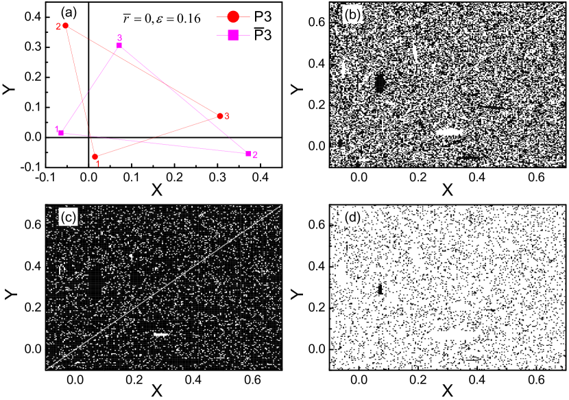
Figure 6: (Color online) Coexistence of two distinct period-3 attractors. (a) Two types of period-3 attractors that coexist in phase space. The basins of attraction of the attractors for (b) $\bar{r}=0$ and $\varepsilon=0.16$, (c) $\bar{r}=0.05$ and $\varepsilon=0.16$, and (d) $\bar{r}=-0.05$ and $\varepsilon=0.16$, where the dark and blank regions represent the basins of attraction of the P3 and $\mathrm{\bar{P}}3$ attractors, respectively.

III.2 Occurrence of periodic attractors of period greater than three

Combining the linear stability and border collision bifurcation analyses, we can obtain the existing conditions of periodic attractors of various periods. Figure 7 shows the theoretical results for periodic attractors of period-4, 7, 8, and 16 for $\bar{r}\geq 0$. We see that, except for the period-4 attractor whose existing condition is determined solely by border collision bifurcation, the emergence and existence of periodic attractors of higher periods are due to the mixed “action” of stability and border collision bifurcation. We also find border collision induced period-doubling bifurcations. For example, a period-8 attractor (P8) arises after the period-4 orbit collides with the discontinuous border, as shown in Fig. 7(c), and a periodic attractor of period-16 emerges after an alternative type of period-8 attractor ($\mathrm{\tilde{P}}$8) collides with the border, as shown in Fig. 7(d). Further, the P8 and $\mathrm{\tilde{P}}$8 attractors can convert into each other through the collision that occurs on the $AB$ curve, as shown in Fig. 7(c). In general, as the period increases, the area of the periodic attractor in the parameter space diminishes quickly.

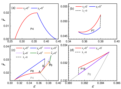
Figure 7: (Color online) Rise of periodic attractors of period greater than three. (a-d) Theoretically obtained stability regions for period-4, period-7, period-8, and period-16 attractors, respectively.

III.3 Globally coupled maps

The occurrence of periodic attractors as a precursor of transition to high-dimensional chaos in nonsmooth systems is a general phenomenon that occurs in systems of globally coupled piecewise linear maps [Eq. (1)]. For such a system, a variety of collective dynamical states can arise. In particular, high-dimensional chaos manifests itself as asynchronous chaos, whereas low-dimensional chaos corresponds to globally synchronous chaos and, in the “buffer” region of periodic attractors, periodic synchronization occurs. The parameter region in which various two-cluster states occur is shown in Fig. 8, which qualitatively agrees with the phase diagram in Fig. 3. Note that, not all stable two-cluster states can be observed in a globally coupled system of finite size. In such a system, multistability FGHY:1996 ; FG:1997 ; KFG:1999 ; KF:2002 ; FG:2003 ; NFS:2011 ; Pateletal:2014 ; PF:2014 ; YHL:2016 ; LG:2017 is common, and the basin of attraction of a stable attractor can have a fractal structure, on which small perturbations can have a significant effect. Certain states are thus not physically observable. Note also that the result in Fig. 3 in fact corresponds to the thermodynamic limit $N\to\infty$, but in Fig. 8, the network size $N$ is finite. This leads to the small discrepancies between Figs. 8 and 3.

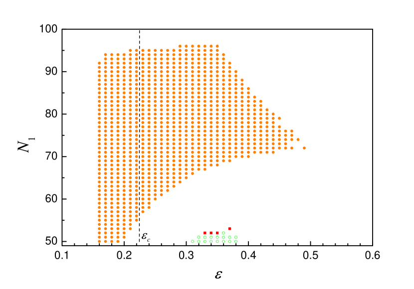
Figure 8: (Color online) Two-cluster state in a globally coupled nonsmooth map system. The size of the network is $N=100$ and $N_{1}$ represents the size of the largest cluster. The two-cluster states of period-3, 4, and 8 are represented by the orange solid, green open, and red square dots, respectively. Each state is obtained using $10^{5}$ random initial conditions.

IV Discussion

Historically, the discoveries of four distinct routes to low-dimensional chaos with one positive Lyapunov exponent: period-doubling Feigenbaum:1978 , intermittency PM:1980 , crisis GOY:1983 , and quasiperiodicity RT:1971 ; GS:1975 ; NRT:1978 , led to fundamental insights into and an understanding of the occurrence of chaotic behaviors in natural systems and henceforth played an important role in the development of nonlinear dynamics. Transition to high-dimensional chaos, chaos with multiple positive Lyapunov exponents, has also been studied but only for smooth dynamical systems HL:1999 ; HL:2000 ; DL:2000 ; PSM:2001 ; PM:2005 . In such systems, a typical route to high-dimensional chaos is that the second Lyapunov exponent passes through zero smoothly from the negative side as a system parameter varies. The generality of this route lies in regarding the underlying dynamical system as consisting of a number of mutually interacting subsystems, some exhibiting low-dimensional chaos. The chaotic subsystems then provide a kind of “driving” to other subsystems. As a bifurcation parameter changes, an additional positive Lyapunov exponent can arise. The nature of chaotic driving stipulates that the second exponent becomes positive in a smooth fashion HL:1999 ; HL:2000 ; DL:2000 , a feature that is characteristic of the transition to chaos in random dynamical systems YOC:1990 ; RHKK:2000 ; LLBS:2002 ; LLBS:2003 .

The main question addressed in this paper is whether transition to high-dimensional chaos in nonsmooth dynamical systems can follow a characteristically different route than that in smooth dynamical systems. The answer is affirmative. In particular, using the paradigmatic setting of coupled nonsmooth maps, we have uncovered a route in which a periodic attractor arises as a precursor to high-dimensional chaos. That is, as a bifurcation parameter is varied from the regime of a low-dimensional chaotic attractor, an interval in which the attractor of the system is periodic occurs, after which a high-dimensional chaotic attractor is born. In a two-dimensional parameter space, the regions of low- and high-dimensional chaos are separated by an open, “bubble” region of periodic attractors. As we have shown, the route to high-dimensional chaos is characteristically different from that in smooth dynamical systems, and the associated feature in the parameter space is also distinct from that about the occurrence of a periodic window (c.f., Fig. 1). Our analysis indicates that the emergence of the “bubble” region can be attributed to border collision bifurcations that occur commonly in nonsmooth dynamical systems. Numerical computations have also revealed that there are parameter regions in which a high-dimensional chaotic attractor can arise smoothly from a low-dimensional one, as in smooth dynamical systems. The general finding is then that, in nonsmooth dynamical systems, smooth and discontinuous routes to high-dimensional chaos coexist in the parameter space. From the perspective of transition to high-dimensional chaos, nonsmooth dynamical systems thus offer richer behaviors than smooth dynamical systems.

References

- (1) E. Lorenz, Deterministic nonperiodic flow. J. Atmos. Sci. 20, 130-141 (1963).
- (2) O. E. Rössler, Equation for continuous chaos. Phys. Lett. A 57, 397-398 (1976).
- (3) K. Ikeda, K. Matsumoto, High-dimensional chaotic behavior in systems with time-delayed feedback. Physica D 29, 223-235 (1987).
- (4) E. Barreto, B. R. Hunt, C. Grebogi, J. A. Yorke, From high dimensional chaos to stable periodic orbits: The structure of parameter space. Phys. Rev. Lett. 78, 4561–4564 (1997).
- (5) Z. E. Musielak, D. E. Musielak, High-dimensional chaos in dissipative and driven dynamical systems. Int. J. Bif. Chaos 19, 2823-2869 (2009).
- (6) I. Ispolatov, V. Madhok, S. Allende, M. Doebeli, Chaos in high-dimensional dissipative dynamical systems. Sci. Rep. 5, 12506 (2015).
- (7) E. Ott, C. Grebogi, J. A. Yorke, Controlling chaos. Phys. Rev. Lett. 64, 1196-1199 (1990).
- (8) S. Boccaletti, C. Grebogi, Y.-C. Lai, H. Mancini, D. Maza, Control of chaos: theory and applications. Phys. Rep. 329, 103-197 (2000).
- (9) D. Auerbach, C. Grebogi, E. Ott, J. A. Yorke, Controlling chaos in high dimensional systems. Phys. Rev. Lett. 69, 3479–3482 (1992).
- (10) C. Grebogi, Y.-C. Lai, Controlling chaos in high dimensions. IEEE Trans. Cir. Sys. 44, 971-975 (1997).
- (11) M. J. Feigenbaum, Quantitative universality for a class of nonlinear transformations. J. Stat. Phys. 19, 25-52 (1978).
- (12) Y. Pomeau, P. Manneville, Intermittent transition to turbulence in dissipative dynamical systems. Commun. Math. Phys. 74, 189-197 (1980).
- (13) C. Grebogi, E. Ott, J. A. Yorke, Crises, sudden changes in chaotic attractors and chaotic transients. Physica D 7, 181-200 (1983).
- (14) D. Ruelle, F. Takens, Nature of turbulence. Commun. Math. Phys. 20, 167 (1971).
- (15) J. P. Gollub, H. L. Swinney, Onset of turbulence in a rotating fluid. Phys. Rev. Lett. 35, 927-930 (1975).
- (16) S. E. Newhouse, D. Ruelle, F. Takens, Occurrence of strange axiom-a attractors near quasiperiodic flows on , is greater than or equal to 3. Commun. Math. Phys. 64, 35-40 (1978).
- (17) M. A. Harrison, Y.-C. Lai, Route to high-dimensional chaos. Phys. Rev. E 59, R3799–R3802 (1999).
- (18) M. A. Harrison, Y.-C. Lai, Bifrucation to high-dimensional chaos. Int. J. Bif. Chaos 10, 1471-1483 (2000).
- (19) R. Davidchack, Y.-C. Lai, Characterization of transition to chaos with multiple positive lyapunov exponents by unstable periodic orbits. Phys. Lett. A 270, 308-313 (2000).
- (20) D. Pazo, E. Sanchez, M. A. Matias, Transition to high-dimensional chaos through quasiperiodic motion. Int. J. Bif. Chaos 11, 2683-2688 (2001).
- (21) D. Pazo, M. A. Matias, Direct transition to high-dimensional chaos through a global bifurcation. Europhys. Lett. 72, 176-182 (2005).
- (22) L. Yu, E. Ott, Q. Chen, Transition to chaos for random dynamical systems. Phys. Rev. Lett. 65, 2935–2938 (1990).
- (23) S. Rim, D.-U. Hwang, I. Kim, C.-M. Kim, Chaotic transition of random dynamical systems and chaos synchronization by common noises. Phys. Rev. Lett. 85, 2304–2307 (2000).
- (24) Z. Liu, Y.-C. Lai, L. Billings, I. B. Schwartz, Transition to chaos in continuous-time random dynamical systems. Phys. Rev. Lett. 88, 124101 (2002).
- (25) Y.-C. Lai, Z. Liu, L. Billings, I. B. Schwartz, Noise-induced unstable dimension variability and transition to chaos in continuous-time random dynamical systems. Phys. Rev. E 67, 026210 (2003).
- (26) B. Xu, Y.-C. Lai, L. Zhu, Y. Do, Experimental characterization of transition to chaos in the presence of noise. Phys. Rev. Lett. 90, 164101 (2003).
- (27) Y.-C. Lai, Symmetry-breaking bifurcation with on-off intermittency in chaotic dynamical systems. Phys. Rev. E 53, R4267-R4270 (1996).
- (28) Y.-C. Lai, Transition from strange nonchaotic to strange chaotic attractors. Phys. Rev. E 53, 57-65 (1996).
- (29) Y.-C. Lai, U. Feudel, C. Grebogi, Scaling behavior of transition to chaos in quasiperiodically driven dynamical systems. Phys. Rev. E 54, 6070-6073 (1996).
- (30) T. Yalcinkaya, Y.-C. Lai, Blowout bifurcation route to strange nonchaotic attractors. Phys. Rev. Lett. 77, 5039-5042 (1996).
- (31) J. M. T. Thompson, R. Ghaffari, Chaotic dynamics of an impact oscillator. Phys. Rev. A 27, 1741–1743 (1983).
- (32) S. W. Shaw, P. J. Holmes, A periodically forced piecewise linear oscillator. J. Sound. Vib. 90, 129-155 (1983).
- (33) G. S. Whiston, Global dynamics of a vibro-impacting linear oscillator. J. Sound. Vib. 118, 395-424 (1987).
- (34) A. B. Nordmark, Non-periodic motion caused by grazing incidence in an impact oscillator. J. Sound. Vib. 145, 279-297 (1991).
- (35) W. Chin, E. Ott, H. E. Nusse, C. Grebogi, Grazing bifurcations in impact oscillators. Phys. Rev. E 50, 4427–4444 (1994).
- (36) F. Casas, W. Chin, C. Grebogi, E. Ott, Universal grazing bifurcations in impact oscillators. Phys. Rev. E 53, 134–139 (1996).
- (37) S. Banerjee, J. A. Yorke, C. Grebogi, Robust chaos. Phys. Rev. Lett. 80, 3049–3052 (1998).
- (38) S. Banerjee, C. Grebogi, Border collision bifurcations in two-dimensional piecewise smooth maps. Phys. Rev. E 59, 4052–4061 (1999).
- (39) S. Banerjee, P. Ranjan, C. Grebogi, Bifurcations in two-dimensional piecewise smooth maps-theory and applications in switching circuits. IEEE Trans. Cir. Syst. I. Fund. Theo. Appl. 47, 633-643 (2000).
- (40) W. Nicola, S. A. Campbell, Nonsmooth bifurcations of mean field systems of two-dimensional integrate and fire neurons. SIAM J. Appl. Dyn. Syst. 15, 391-439 (2016).
- (41) W. Nicola, B. Tripp, M. Scott, Obtaining arbitrary prescribed mean field dynamics for recurrently coupled networks of type-i spiking neurons with analytically determined weights. Front. Comp. Neurosci. 10, 15 (2016).
- (42) H. E. Nusse, J. A. Yorke, Border-collision bifurcations including “period two to period three” for piecewise smooth systems. Physica D 57, 39-57 (1992).
- (43) H. E. Nusse, E. Ott, J. A. Yorke, Border-collision bifurcations: An explanation for observed bifurcation phenomena. Phys. Rev. E 49, 1073–1076 (1994).
- (44) M. Dutta, H. E. Nusse, E. Ott, J. A. Yorke, G. Yuan, Multiple attractor bifurcations: A source of unpredictability in piecewise smooth systems. Phys. Rev. Lett. 83, 4281–4284 (1999).
- (45) J. Lv, T.-S. Zhou, G. R. Chen, X.-S. Yang, Generating chaos with a switching piecewise-linear controller. Chaos 12, 344-349 (2002).
- (46) M. A. Hassouneh, E. H. Abed, H. E. Nusse, Robust dangerous border-collision bifurcations in piecewise smooth systems. Phys. Rev. Lett. 92, 070201 (2004).
- (47) A. Ganguli, S. Banerjee, Dangerous bifurcation at border collision: When does it occur? Phys. Rev. E 71, 057202 (2005).
- (48) V. Avrutin, M. Schanz, S. Banerjee, Codimension-three bifurcations: Explanation of the complex one-, two-, and three-dimensional bifurcation structures in nonsmooth maps. Phys. Rev. E 75, 066205 (2007).
- (49) Y.-H. Do, Y.-C. Lai, Multistability and arithmetically period-adding bifurcations in piecewise smooth dynamical systems. Chaos 18, 043107 (2008).
- (50) B. Christiansen, et al., Phase diagram of a modulated relaxation oscillator with a finite resetting time. Phys. Rev. A 45, 8450–8456 (1992).
- (51) S.-X. Qu, S. Wu, D.-R. He, Multiple devil’s staircase and type-v intermittency. Phys. Rev. E 57, 402–411 (1998).
- (52) J. Wang, et al., Characteristics of a piecewise smooth area-preserving map. Phys. Rev. E 64, 026202 (2001).
- (53) Y.-C. Lai, D.-R. He, Y.-M. Jiang, Basins of attraction in piecewise smooth hamiltonian systems. Phys. Rev. E 72, 025201 (2005).
- (54) K. Yang, X. Wang, S.-X. Qu, Cyclic synchronous patterns in coupled discontinuous maps. Phys. Rev. E 92, 022905 (2015).
- (55) K. Kaneko, Chaotic but regular posi-nega switch among coded attractors by cluster-size variation. Phys. Rev. Lett. 63, 219–223 (1989).
- (56) K. Kaneko, Clustering, coding, switching, hierarchical ordering, and control in a network of chaotic elements. Physica D 41, 137 - 172 (1990).
- (57) K. Kaneko, Globally coupled chaos violates the law of large numbers but not the central-limit theorem. Phys. Rev. Lett. 65, 1391–1394 (1990).
- (58) A. Pikovsky, O. Popovych, Y. Maistrenko, Resolving clusters in chaotic ensembles of globally coupled identical oscillators. Phys. Rev. Lett. 87, 044102 (2001).
- (59) O. Popovych, Y. Maistrenko, E. Mosekilde, Loss of coherence in a system of globally coupled maps. Phys. Rev. E 64, 026205 (2001).
- (60) O. Popovych, Y. Maistrenko, E. Mosekilde, Role of asymmetric clusters in desynchronization of coherent motion. Phys. Lett. A 302, 171 - 181 (2002).
- (61) A. F. Taylor, et al., Clusters and switchers in globally coupled photochemical oscillators. Phys. Rev. Lett. 100, 214101 (2008).
- (62) A. Polynikis, M. di Bernardo, S. J. Hogan, Synchronizability of coupled pwl maps. Chaos Soli. Frac. 41, 1353-1367 (2009).
- (63) A. Pikovsky, M. Rosenblum, Dynamics of globally coupled oscillators: Progress and perspectives. Chaos 25, 097616 (2015).
- (64) K. Kaneko, From globally coupled maps to complex-systems biology. Chaos 25, 097608 (2015).
- (65) U. Feudel, C. Grebogi, B. R. Hunt, J. A. Yorke, Map with more than 100 coexisting low-period periodic attractors. Phys. Rev. E 54, 71–81 (1996).
- (66) U. Feudel, C. Grebogi, Multistability and the control of complexity. Chaos 7, 597-604 (1997).
- (67) S. Kraut, U. Feudel, C. Grebogi, Preference of attractors in noisy multistable systems. Phys. Rev. E 59, 5253–5260 (1999).
- (68) S. Kraut, U. Feudel, Multistability, noise, and attractor hopping: The crucial role of chaotic saddles. Phys. Rev. E 66, 015207 (2002).
- (69) U. Feudel, C. Grebogi, Why are chaotic attractors rare in multistable systems? Phys. Rev. Lett. 91, 134102 (2003).
- (70) C. N. Ngonghala, U. Feudel, K. Showalter, Extreme multistability in a chemical model system. Phys. Rev. E 83, 056206 (2011).
- (71) M. S. Patel, et al., Experimental observation of extreme multistability in an electronic system of two coupled Rössler oscillators. Phys. Rev. E 89, 022918 (2014).
- (72) A. N. Pisarchik, U. Feudel, Control of multistability. Phys. Rep. 540, 167-218 (2014).
- (73) L. Ying, D. Huang, Y.-C. Lai, Multistability, chaos, and random signal generation in semiconductor superlattices. Phys. Rev. E 93, 062204 (2016).
- (74) Y.-C. Lai, C. Grebogi, Quasiperiodicity and suppression of multistability in nonlinear dynamical systems. Euro. Phys. J. Spec. Top. 226, 1703-1719 (2017).