Adversarial Perturbations Against Real-Time Video Classification Systems

Abstract.

Recent research has demonstrated the brittleness of machine learning systems to adversarial perturbations. However, the studies have been mostly limited to perturbations on images and more generally, classification that does not deal with temporally varying inputs. In this paper we ask ”Are adversarial perturbations possible in real-time video classification systems and if so, what properties must they satisfy?” Such systems find application in surveillance applications, smart vehicles, and smart elderly care and thus, misclassification could be particularly harmful (e.g., a mishap at an elderly care facility may be missed). We show that accounting for temporal structure is key to generating adversarial examples in such systems. We exploit recent advances in generative adversarial network (GAN) architectures to account for temporal correlations and generate adversarial samples that can cause misclassification rates of over 80 % for targeted activities. More importantly, the samples also leave other activities largely unaffected making them extremely stealthy. Finally, we also surprisingly find that in many scenarios, the same perturbation can be applied to every frame in a video clip that makes the adversary’s ability to achieve misclassification relatively easy.

1. Introduction

Deep Neural Networks (DNN) have found an increasing role in real world applications for the purposes of real-time video classification. Examples of such applications include video surveillance (Sultani et al., 2018), self driving cars (Kataoka et al., 2018a), health-care (Vision, 2016), etc. To elaborate, video surveillance systems capable of automated detection of undesired human behaviors (e.g., violence) can trigger alarms and drastically reduce information workloads on human operators. Without the assistance of DNN-based classifiers, human operators will need to simultaneously view and assess footage from a large number of video sensors. This can be a difficult and exhausting task, and comes with the risk of missing behaviors of interest and slowing down decision cycles. In self-driving cars, video classification has been used to understand pedestrian actions and make navigation decisions (Kataoka et al., 2018a). Real-time video classification systems have also been deployed for automatic “fall detection” in elderly care facilities (Vision, 2016), and abnormal detection around automated teller machines (Tripathi et al., 2016). All of these applications directly relate to the physical security or safety of people and property. Thus, stealthy attacks on such real-time video classification systems are likely to cause unnoticed pecuniary loss and compromise personal safety.

Recent studies have shown that virtually all DNN-based systems are vulnerable to well-designed adversarial inputs (Moosavi-Dezfooli et al., 2017; Moosavi Dezfooli et al., 2016; Sharif et al., 2016; Goodfellow et al., 2014a; Szegedy et al., 2013), which are also referred to as adversarial examples. Szegedy et al. (Szegedy et al., 2013) showed that adversarial perturbations that are hardly perceptible to humans can cause misclassification in DNN-based image classifiers. Goodfellow et al. (Goodfellow et al., 2014b) analyzed the potency of realizing adversarial samples in the physical world. Moosavi et al. (Moosavi-Dezfooli et al., 2017) and Mopuri et al. (Mopuri et al., 2017b) introduced the concept of “image-agnostic” perturbations. As such, the high level question that we try to answer in this paper is “Is it possible to launch stealthy attacks against DNN-based real-time video classification systems, and if so how?”

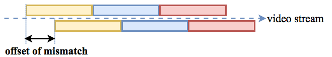
(a) This figure depicts a scenario where there is a mismatch between the clip an attacker views to generate a perturbation, and the clip a classifier views for classification.

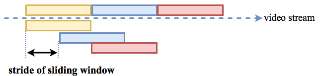
(b) This figure displays a scenario where the stride of the sliding window is smaller than the size of a clip. In such a case, the attacker will not know what perturbation to use on a frame, as the frame can be selected in multiple input clips used in classification.

Figure 4. The sliding window used to capture clips that are input to the video classification system

Attacking a video classifier is more complex than attacking an image classifier, because of the presence of the temporal dimension in addition to the spatial dimensions present in 2D images. Specifically, attacking a real-time video classifier poses additional challenges. First, because the classification is performed in real-time, the corresponding perturbations also need to be generated on-the-fly with the same frame rate which is extremely computationally intensive. Second, to make the attack stealthy, attackers would want to add perturbations on the video in such a way that they will only cause misclassification for the targeted (possibly malicious) actions, while keep the classification of other actions unaffected. In a real-time video stream, since the activities change across time, it is hard to identify online and in one-shot (Fanello et al., 2013), the target frames on which to add perturbations. Third, video classifiers use video clips (a set of frames) as inputs (Fanello et al., 2013; Tripathi et al., 2016). As video is captured, it is broken up into clips and each clip is fed to the classifier. As a result, even if attackers are aware of the length of each clip (a hyper-parameter of the classifier), it is hard to predict when each clip begins and ends. Therefore, if they generate perturbations for a clip using traditional methods (e.g., gradient descent), the perturbations might not work because they are not aligned with the real clip the classifier is using (Please see Figure 4 and the associated discussion for more details).

In this paper, our first objective is to investigate how to generate adversarial perturbations against real-time video classification systems by overcoming the above challenges. We resolve the first (real-time) challenge by using universal perturbations (Moosavi-Dezfooli et al., 2017). Universal perturbations allow us to affect the classification results using a (single) set of perturbations generated off-line. Because they work on unseen inputs they preclude the need for intensive on-line computations to generate perturbations for every incoming video clip. To generate such universal perturbations, we leverage the generative adversarial network (GAN) (Goodfellow et al., 2014a) architecture.

However, adding universal perturbations on all the frames of the video can cause the misclassification of all the actions in the video stream. This may expose the attack as the results may not make sense (e.g., many people performing rare actions). To make the attack stealthy, we introduce the novel concept of dual purpose universal perturbations, which we define as universal perturbations which only cause the misclassification for inputs belonging to the target class, while minimize, or ideally, have no effect on the classification results for inputs belonging to the other classes.

Dual purpose perturbations by themselves do not provide high success rates in terms of misclassification because of challenge three, which is that the mis-alignment of the boundaries of perturbations with respect to the real clip boundaries (input to the classifier) significantly affects the misclassification success rates. To solve this problem, we introduce a new type of perturbation that we call the Circular Universal Dual Purpose Perturbations (C-DUP). The C-DUP is a 3D perturbation (i.e., a perturbation clip composed of a sequence of frames), which is a valid perturbation on a video regardless of the start and end of each clip. In other words, it works on all cyclic permutations of frames in a clip. To generate the C-DUP, we make significant changes to the baseline GAN architecture. In particular, we add a new unit to generate circular perturbations, that is placed between the generator and the discriminator (as discussed later). We demonstrate that the C-DUP is very stable and effective in achieving real-time stealthy attacks on video classification systems.

After demonstrating the feasibility of stealthy attacks against real-time video classification systems, our second objective is to investigate the effect of the temporal dimension. In particular, we investigate the feasibility of attacking the classification systems using a simple and light 2D perturbation which is applied across all the frames of a video. By tweaking our generative model, we are able to generate such perturbations which we name as 2D Dual Purpose Universal Perturbations (2D-DUP). These perturbations work well on a sub-set of videos, but not all. We will discuss the reasons for these 2D attacks in § 6.3.

Our Contributions: In brief, our contributions in this paper are:

• We provide a comprehensive analysis on the challenges in crafting adversarial perturbations for real-time video classifiers. We empirically identify what we call the boundary effect phenomenon in generating adversarial perturbations against video (see § 6).

• We design and develop a generative framework to craft two types of stealthy adversarial perturbations against real-time video classifiers, viz., circular dual purpose universal perturbation (C-DUP) and 2D dual purpose universal perturbation (2D-DUP). These perturbations are agnostic to (a) the video captured (universal) and (b) the temporal sequence of frames in the clips input to the video classification system (resistance to cyclic permutations of frames in a clip).

• We demonstrate the potency of our adversarial perturbations using two different video datasets. In particular, the UCF101 dataset captures coarse-grained activities (human actions such as applying eye makeup, bowling, drumming) (Soomro et al., 2012). The Jester dataset captures fine-grained activities (hand gestures such as sliding hand left, sliding hand right, turning hand clockwise, turning hand counterclockwise) (Dataset, 2016). We are able to launch stealthy attacks on both datasets with over a 80 % misclassification rate, while ensuring that the other classes are correctly classified with relatively high accuracy.

2. Background

In this section, we provide the background relevant to our work. Specifically, we discuss how a real-time video classification system works and what standard algorithms are currently employed for action recognition. We also discuss generative adversarial networks (GANs) in brief.

2.1. Real-time video-based classification systems

DNN based video classification systems are being increasingly deployed in real-world scenarios. Examples include fall detection in elderly care (Foroughi et al., 2008), abnormal event detection on campuses (Vision, [n. d.]b, [n. d.]a), security surveillance for smart cities (Vision, [n. d.]c), and self-driving cars (Kataoka et al., 2018a, b). Given an input real-time video stream, which may contain one or more known actions, the goal of a video classification system is to correctly recognize the sequence of the performed actions. Real-time video classification systems commonly use a sliding window to analyze a video stream (Fanello et al., 2013; Tripathi et al., 2016). The classifier computes an output score for each class in each sliding window. The sliding window moves with a stride. Moving in concert with the sliding window, one can generate “score curves” for each action class. Note that the scores for all the action classes evolve with time. The score curves are then smoothed (to remove noise) as shown in Figure 1. With the smoothed score curves, the on-going actions are predicted online. From the figure one can see that, the real-time video classification system is fooled if one can make the classifier output a low score for the true class in each sliding window; with this, the true actions will not be recognized.

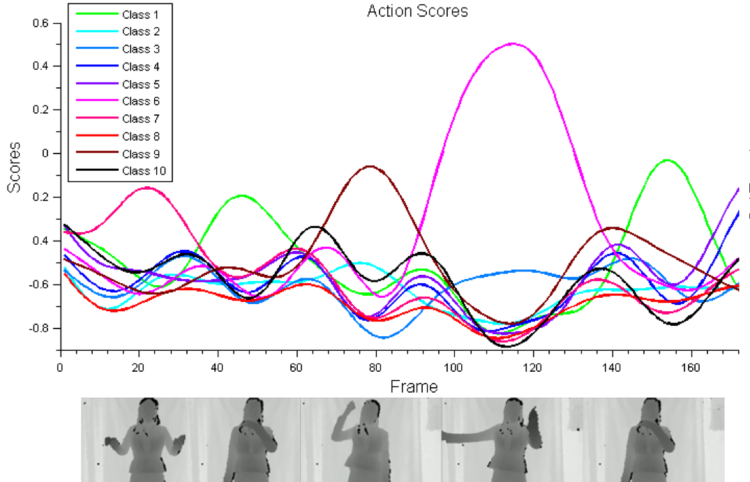
Figure 1. This figure (Fanello et al., 2013) illustrates the score curves computed by a video classifier with a sliding window for every class. Real-time video classification systems use these score curves to do online action recognition.

Figure 2. The C3D architecture(Tran et al., 2015). C3D net has 8 convolution, 5 max-pooling, and 2 fully connected layers, followed by a softmax output layer. All 3D convolution kernels are $3\times 3\times 3$ with a stride (Tran et al., 2015) of 1 in both spatial and temporal dimensions. The number of filters are shown in each box. The 3D pooling layers are represented from pool1 to pool5. All pooling kernels are $2\times 2\times 2$, except for pool1, which is $1\times 2\times 2$. Each fully connected layer has 4096 output units.

2.2. The C3D classifier

Next, we describe what is called the C3D classifier (Tran et al., 2015), a state of the art classifier that we target in our paper.

DNNs and in particular convolutional neural networks (CNNs) are being increasingly applied in video classification. Among these, spatio-temporal networks like C3D (Tran et al., 2015) and two-stream networks like I3D (Carreira and Zisserman, 2017) outperform other network structures(Herath et al., 2017; Gu et al., 2017). Without the requirement of non-trivial pre-processing on the video stream, spatio-temporal networks demonstrate high efficiency; among these, C3D is the start-of-art model (Gu et al., 2017).

The C3D model is generic, which means that it can differentiate across different types of videos (e.g., videos of actions in sports, actions involving pets, actions relating to food etc.). It also provides a compact representation that facilitates scalability in processing, storage, and retrieval. It is also extremely efficient in classifying video streams (needed in real-time systems).

Given its desirable attributes and popularity, without loss of generality, we use the C3D model as our attack target in this paper. The C3D model is based on 3D ConvNet (a 3D CNN) (Karpathy et al., 2014; Tran et al., 2015; Varol et al., 2017), which is very effective in modeling temporal information (because it employs 3D convolution and 3D pooling operations).

The architecture and hyperparamters of C3D are shown in Figure 2. The input to the C3D classifier is a clip consisting of 16 consecutive frames. This means that upon using C3D, the sliding window size is 16. Both the height and the width of each frame are 112 pixels and each frame has 3 (RGB) channels. The last layer of C3D is a softmax layer that provides a classification score with respect to each class.

2.3. Generative Adversarial Networks and their relevance

Generative Adversarial Networks (GANs) (Goodfellow et al., 2014a) were initially developed to generate synthetic content (and in particular, images) that conformed with the space of natural content (Zhu et al., 2016; Huang et al., 2017). Recently, there has also been work on using GANs for generating synthetic videos (Vondrick et al., 2016). The GAN consists of two components viz., a generator or generative model that tries to learn the training data distribution and a discriminator or discriminative model that seeks to distinguish the generated distribution from the training data distribution.

To elaborate, consider the use of a GAN for video generation. An archtecture for this purpose is shown in 3(a). The generator $G$, learns a map from a random vector $z$ in latent space, to a natural video clip $V$; in other words, $G(z)=V$, where $z$ is usually sampled from a simple distribution such as a Gaussian distribution ($N(0,1)$) or a uniform distribution ($U(-1,1)$). The discriminator $D$ takes a video clip as input (either generated or natural), and outputs the probability that it is from the training data (i.e., the probability that the video clip is natural). The interactions between $G$ and $D$ are modeled as a game and in theory, at the end $G$ must be able to generate video clips from the true training set distribution.

Recently, a GAN-like architecture has been used to generate adversarial perturbations on images (Mopuri et al., 2017b) . The authors of  (Mopuri et al., 2017b) keep a trained discriminator fixed; its goal is to classify the inputs affected by the perturbations from the generator. The generator learns from the discriminator classifications to modulate its perturbations. Similarly, we apply the GAN-like architecture wherein the objective is to allow the generator to learn a distribution for candidate perturbations that can fool our discriminator. Our model incorporates significant extensions to the GAN structure used in (Mopuri et al., 2017b) to account for the unique properties of video classification that were discussed earlier.

3. Threat Model and Datasets

In this section, we describe our threat model. We also provide a brief overview of the datasets we chose for validating our attack models.

3.1. Threat model

We consider a white-box model for our attack, i.e., the adversary has access to the training datasets used to train the video classification system, and has knowledge of the deep neural network model the real-time classification system uses. We also assume that the adversary is capable of injecting perturbations in the real-time video stream. In particular, we assume the adversary to be a man-in-the-middle that can intercept and add perturbations to streaming video (Lab, 2014), or that it could have previously installed a malware that is able to add perturbation prior to classification (Net, 2016).

We assume that the goal of the adversaries is to launch stealthily attacks, i.e., they want the system to only misclassify the malicious actions without affecting the recognition of the other actions. So, we consider two attack goals. First, given a target class, we want all the clips from this class to be misclassified by the real-time video classifier. Second, for all the clips from other (non-target) classes, we want the classifier to correctly classify them.

3.2. Our datasets

We use the human action recognition dataset UCF-101 (Soomro et al., 2012) and the hand gesture recognition dataset 20BN-JESTER dataset (Jester) (Dataset, 2016) to validate our attacks on video classification systems. We use these two datasets because they represent two kinds of classification, i.e., coarse-gained and fine-grained action classification.

The UCF 101 dataset: The UCF 101 dataset used in our experiments is the standard dataset collected from Youtube. It includes 13320 videos from 101 human action categories (e.g., applying lipstick, biking, blow drying hair, cutting in the kitchen etc.). The videos collected in this dataset have variations in camera motion, appearance, background, illumination conditions etc. Given the diversity it provides, we consider the dataset to validate the feasibility of our attack model on coarse-gained actions. There are three different (pre-existing) splits (Soomro et al., 2012) in the dataset; we use split 1 for both training and testing, in our experiments. The training set includes 9,537 video clips and the testing set includes 3,783 video clips.

The Jester dataset: The 20BN-JESTER dataset (Jester) is a recently collected dataset with hand gesture videos. These videos are recorded by crowd-source workers performing 27 kinds of gestures (e.g., sliding hand left, sliding two fingers left, zooming in with full hand, zooming out with full hand etc.). We use this dataset to validate our attack with regards to fine-grained actions. Since this dataset does not currently provide labels for the testing set, we use the validation set as our testing set (i.e., apply our perturbations on the validation set). The training set has 148,092 short video clips and our testing set has 14,787 short video clips.

4. Generating perturbations for real-time video stream

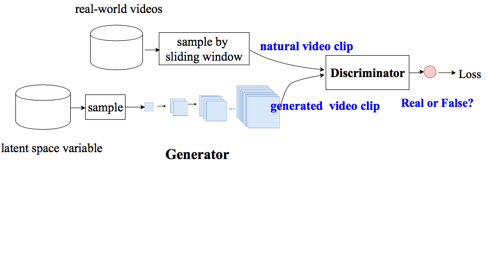
(a) GAN Architecture

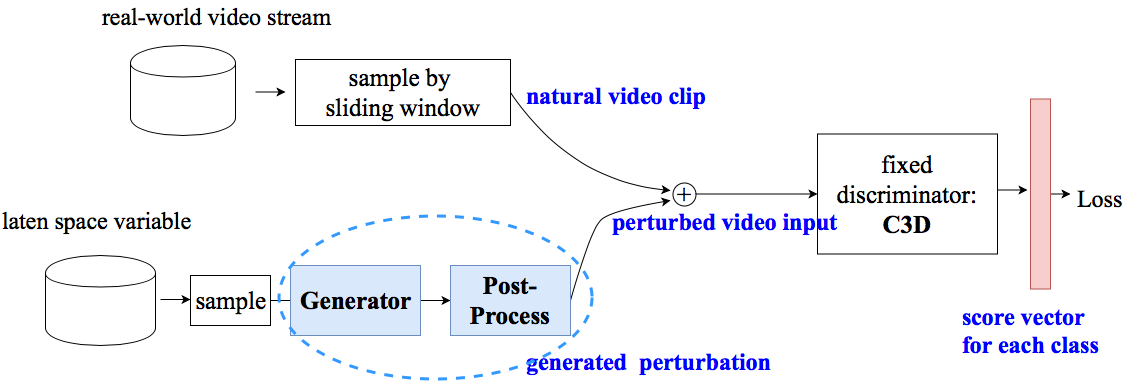
(b) Our Architecture

Figure 3. This figure compares our architecture with traditional GAN architectures. Our architecture is different fromtraditional GAN in the following aspects: 1) The discriminator is a pre-trained classifier we attack, whose goal is to classify videos, and not to distinguish between the natural and synthesized inputs; 2) The generator generates perturbations, and not direct inputs to the discriminator, and the perturbed training inputs are fed to discriminator; 3) The learning objective is to let the discriminator misclassify the perturbed inputs.

From the adversary’s perspective, we first consider the challenge of attacking a real-time video stream. In brief, when attacking an image classification system, the attackers usually take the following approach. First, they obtain the target image that is to be attacked with its true label. Next, they formulate a problem wherein they try to compute the “minimum” noise that is to be added in order to cause a mis-classification of the target. The formulation takes into account the function of the classifier, the input image, and its true label. In contrast, in the context of real-time video classification, the video is not available to the attackers a priori. Thus, they will need to create perturbations that can effectively perturb an incoming video stream, whenever a target class is present.

Our approach is to compute the perturbations offline and apply them online. Since we cannot predict what is captured in the video, we need perturbations which work with unseen inputs. A type of perturbations that satisfies this requirement is called the Universal Perturbation (UP), which has been studied in the context of generating adversarial samples against image classification systems (Mopuri et al., 2017b; Moosavi-Dezfooli et al., 2017). In particular, Mopuri et al. , have developed a generative model that learns the space of universal perturbations for images using a GAN-like architecture.

Inspired by this work, we develop a similar architecture, but make modifications to suit our objective. Our goal is to generate adversarial perturbations that fool the discriminator instead of exploring the space for diverse UPs. In addition, we retrofit the architecture to handle video inputs. Our architecture is depicted in 3(b). It consists of three main components: 1) a 3D generator which generates universal perturbations; 2) a post-processor, which for now does not do anything but is needed to solve other challenges described in subsequent sections; and 3) a pre-trained discriminator for video classification, e.g., the C3D model described in § 2.2. Note that unlike in traditional GANs wherein the generator and the discriminator are trained together, we only train the generator to generate universal perturbations to fool a fixed type of discriminator.

The 3D generator in our model is configured to use 3D deconvolution layers and provide 3D outputs as shown in Figure 8. Specifically, it generates a clip of perturbations, whose size is equal to the size of the video clips taken as input by the C3D classifier. To generate universal perturbations, the generator first takes a noise vector $z$ from a latent space. Next, It maps $z$ to a perturbation clip $p$, such that, $G(z)=p$. It then adds the perturbations on a training clip $x$ to obtain the perturbed clip $x+p$. Let $c(x)$ be the true label of $x$. This perturbed clip is then input to the C3D model which outputs the score vector $Q(x+p)$ (for the perturbed clip). The classification should ensure that the highest score corresponds to the true class ($c(x)$ for input $x$) in the benign setting. Thus, the attacker seeks to generate a $p$ such that the C3D classifier outputs a low score to the $c(x)$th element in $Q$ vector (denoted as $Q_{c(x)}$) for $x+p$. In other words, this means that after applying the perturbation, the probability of mapping $x$ to class $c(x)$ is lower than the probability that it is mapped to a different class (i.e., the input is not correctly recognized).

We seek to make this perturbation clip $p$ “a universal perturbation”, i.e., adding $p$ to any input clip belonging to the target class would cause misclassification. This means that we seek to minimize the sum of the cross-entropy loss over all the training data as per Equation 1. Note that the lower the cross-entropy loss, the higher the divergence of the predicted probability from the true label (Huang et al., 2017).

(1) $$\underset{G}{\text{minimize}}\quad\sum_{x\in X}{-\log[1-Q_{c(x)}(x+G(z)]}$$

When the generator is being trained, for each training sample, it obtains feedback from the discriminator and adjusts its parameters to cause the discriminator to misclassify that sample. It tries to find a perturbation that works for every sample from the distribution space known to the discriminator. At the end of this phase, the attacker will have a generator that outputs universal perturbations which can cause the misclassification on any incoming input sample from the same distribution (as that of the training set). However, as discussed next, just applying the universal perturbations alone will not be sufficient to carry out a successful attack. In particular, the attack can cause unintended clips to be misclassified as well, which could compromise our stealth requirement as discussed next in §5.

5. making perturbations stealthy

Blindly adding universal perturbations will affect the classification of clips belonging to other non-targeted classes. This may raise alarms, especially if many of such misclassifications are mapped on to rare actions. Thus, while causing the target class to be misclassified, the impact on the other classes must be imperceptible. This problem can be easily solved when dealing with image recognition systems since images are self-contained entities, i.e., perturbations can be selectively added on target images only. However, video inputs change temporally and an action captured in a set of composite frames may differ from that in the subsequent frames. It is thus hard to a priori identify (choose) the frames relating to the target class, and add perturbations specifically on them. For example, consider a case with surveillance in a grocery store. If attackers seek to misclassify an action related to shoplifting and cause this action to go undetected, they do not have a priori knowledge about when this action will be captured. And adding universal perturbations blindly could cause mis-classifications of other actions (e.g., other benign customer actions may be mapped onto shoplifting actions thus triggering alarms).

Since it is hard (or even impossible) to a priori identify the frame(s) that capture the intended actions and choose them for perturbation, the attackers need to add perturbations on each frame. However, to make these perturbations furtive, they need to ensure that the perturbations added only mis-classifies the target class while causing other (non-targeted) classes to be classified correctly. We name this unique kind of universal perturbations as “Dual-Purpose Universal Perturbations” or DUP for short.

In order to realize DUPs, we have to guarantee that for the input clip $x_{t}$, if it belongs to the target class (denote the set of inputs from target class as $T$), the C3D classifier returns a low score with respect to the correct class $c(x_{t})$, i.e., $Q_{c(x_{t})}$. For input clips $x_{s}$ that belongs to other (non-target) classes (denote the set of inputs from non-target classes as $S$, thus, $S=X-T$), the model returns high scores with regards to their correct mappings ($Q_{c(x_{s})}$). To cause the generator to output DUPs, we refine the optimization problem in Equation 1 as shown in Equation 2:

(2) $$\underset{G}{\text{minimize}} \lambda\times\sum_{x_{t}\in T}{-\log[1-Q_{c(x_{t})}(x_{t}+G(z))]}$$

$$+\sum_{x_{s}\in S}{-\log[Q_{c(x_{s})}(x_{s}+G(z))]}$$

The first term in the equation again relates to minimizing the cross-entropy of the target class, while the second term maximizes the cross-entropy relating to each of the other classes. The parameter $\lambda$ is the weight applied with regards to the misclassification of the target class. For attacks where stealth is more important, we may use a smaller $\lambda$ to guarantee that the emphasis on the misclassification probability of the target class is reduced while the classification of the non-target classes are affected to the least extent possible.

6. The time machine: handling the temporal dimension

The final challenge that the attackers will need to address in order to effectively generate adversarial perturbations against real-time video classification systems is to handle the temporal structure that exists across the frames in a video. In this section, we first discuss why directly applying existing methods that target images to generate perturbations against video streams do not work. Subsequently, we propose a new set of perturbations that overcome this challenge.

6.1. The boundary effect

The input to the video classifier is a clip of a sequence of frames. As discussed earlier, given an input clip, it is possible to generate perturbations for each frame in that clip. However, the attacker cannot a priori determine the clip boundaries used by the video classifier. In particular, as discussed in § 2.1, there are three hyper-parameters that are associated with a sliding window of a video classifier. They are the window size, the stride and the starting position of the clip. All three parameters affect the effectiveness of the perturbations. While the first two parameters are known to a white-box attacker, the last parameter is an artifact of when the video clip is captured and input to the classifier and cannot be known a priori.

The perturbation that is to be added to a frame depends on the relative location of the frame within the clip. In other words, if the location of the frame changes because of a temporally staggered clip, the perturbation needs to adjusted accordingly. Thus at a high level, the boundaries of the clips used by the classifier will have an effect on the perturbations that need to be generated. We refer to this phenomenon as the boundary effect. To formalize the problem, let us suppose that there is a video stream represented by $\{...,f_{i-2},f_{i-1},f_{i},f_{i+1},f_{i+2},...\}$ where each $f_{j}$ represents a frame. The perturbation on $f_{i}$ that is generated based on the clip [$f_{i},f_{i+1},\cdots,f_{i+w-1}$] to achieve misclassification of a target action, will be different from the one generated based on the temporally staggered clip $[f_{i-1},f_{i},f_{i+1}\cdots,f_{i+w-2}]$ to achieve the same purpose.

To exemplify this problem, we consider using the traditional methods to attack C3D model. In particular, we use the API from the CleverHans repository (Papernot et al., 2016a) to generate video perturbations. Note that, the perturbations generated by CleverHans are neither universal nor dual-purpose; they simply generate a specific perturbation given a specific input clip. We use the basic iteration methods with default parameters. Our approach is as follows. We consider all the videos in the UCF-101 testing set. We consider different boundaries for the clips in the videos (temporally staggered versions of the clips) and use the Python libraries from CleverHans to generate perturbations for each staggered version. Note that the sliding window size for C3D is 16 and thus, there are 16 staggered versions. We choose a candidate frame, and compute the correlations between the perturbations added in the different staggered versions. Specifically, the perturbations are tensors and the normalized correlation between two perturbations is the inner product of the unit-normalized tensors representing the perturbations.

We represent the average normalized correlations in the perturbations (computed across all videos and all frames) for different offsets (i.e., the difference in the location of the candidate frame in the two staggered clips) in the matrix shown in Figure 5. The row index and the column index represent the location of the frames in the two staggered clips. For example, the entry corresponding to $\{7,7\}$ represents the case where the frame considered was the $7^{th}$ frame in the two clips. In this case, clearly the correlation is 1.00. However, we see that the correlations are much lower if the positions of the same frame in the two clips are different. As an example, consider the entry $\{5,9\}$: its average normalized correlation is 0.39, which indicates that the perturbations that CleverHans adds in the two cases are quite different.

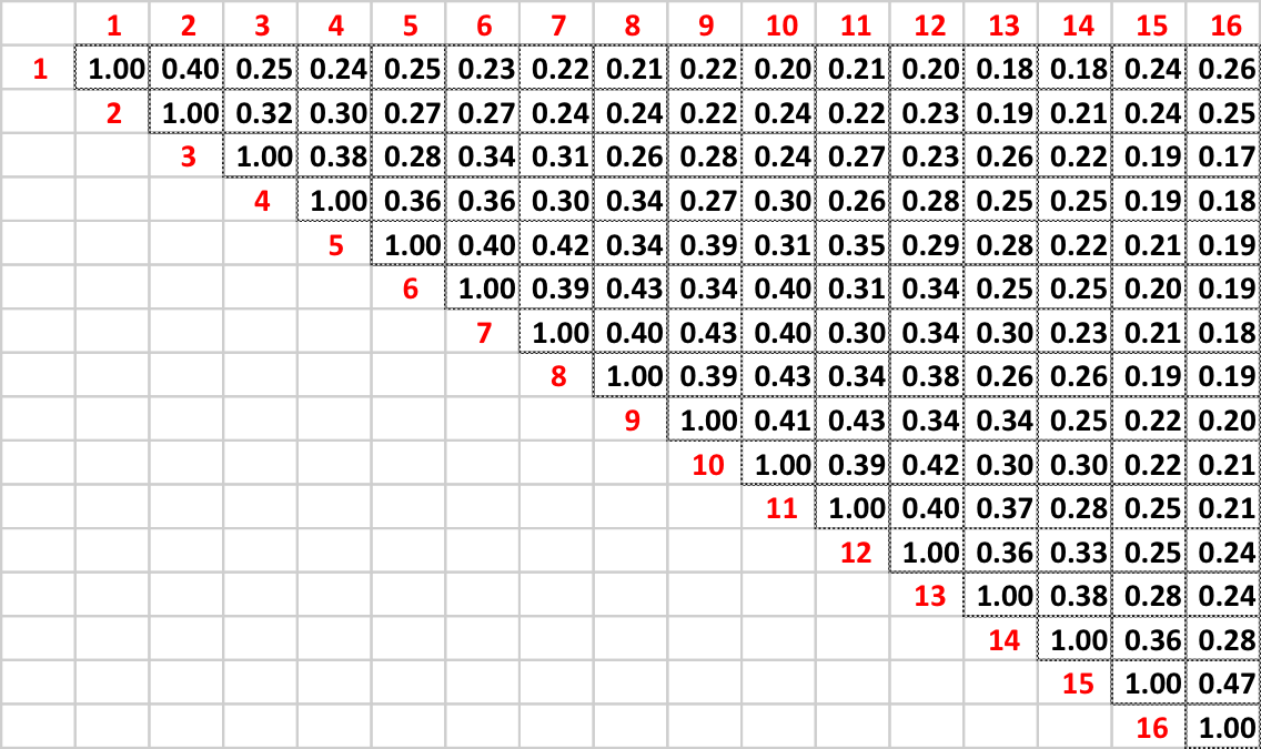
Figure 5. The average normalized correlation matrix computed with perturbations generated using the basic iteration API from CleverHans. Both row and column represent the location of frame in clips and the value represents the correlation between perturbations on the same frames but generated when that frame located in different positions in the two temporally staggered clips.

In Figure 6, we show the average magnitude of perturbations added (over all frames and all videos), when the target frame is at different locations within a clip. The abscissa depicts the frame position, and the ordinate represents the magnitude of the average perturbation. We observe that the magnitude of the perturbation on the first and last few frames are larger than those in the middle. We conjecture this is because the difference in perturbation between consecutive frame locations are similar (because the clips with small temporal offsets are similar); but as the frame location differs by a lot, the perturbation difference will again go up (clips with larger offsets will be more diverse).

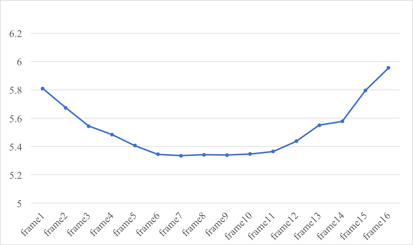
Figure 6. Magnitude of perturbation on each frame: The x axis is the frame position, and the y axis is the magnitude of average perturbation on the frame.

We further showcase the impact of the boundary effect by measuring the degradation in attack efficacy due to mismatches between the anticipated start point when the perturbation is generated and the actual start point when classifying the clip (as shown in 4(a)). Figure 7 depicts the results. The abscissa is the offset between the clip considered for perturbation generation and the clip used in classification. We can see that as the distance between the two start points increases, the attack success rate initially degrades but increases again as the clip now becomes similar to the subsequent clip. For example, if the offset is 15, the clip chosen is almost identical to the subsequent clip.

The boundary effect is also experienced when the stride used by the classifier is smaller than the clip size. In brief, stride refers to the extent to which the receiver’s sliding window advances when considering consecutive clips during classification. If the stride is equal to the clip size, there is no overlap between the clips that are considered as inputs for classification. On the other hand, if the stride is smaller than the size of the clip, which is often the case (Tran et al., 2015; Carreira and Zisserman, 2017; Fanello et al., 2013; Tripathi et al., 2016), the clips used in classification will overlap with each other as shown in 4(b). A stride that is smaller than the clip size will cause the same problem discussed above with respect to the temporal offset between the attackers’ anticipation of the start point and the actual start point of the classifier. As evident from the figure, such a stride induces an offset, and this results in the same behaviors that we showcased above.

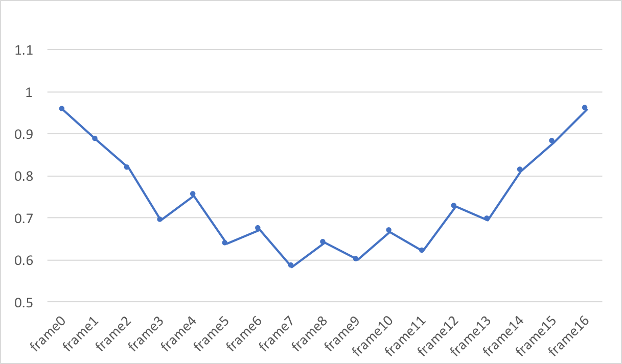
Figure 7. Attack success rate when there is mismatch. The x axis is the offset between the clip generating perturbation and the clip tested. The y axis is the attack success rate.

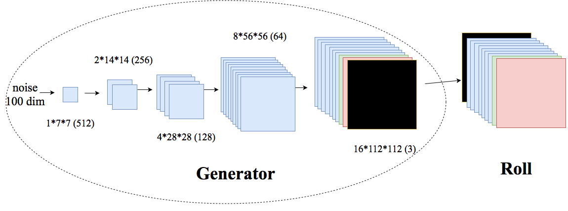
Figure 8. This figure illustrates the Generator and Roll for generating C-DUP. 1) The generator takes a noise vector as input, and outputs a perturbation clip with 16 frames. The output size for each layer is shown as $\text{temporal dimension}\times\text{horizontal spatial dimension}\times\text{vertical spatial dimension}\times\text{number of channels}$. 2) The roll part shifts the perturbation clip by some offset. The figure shows one example where we roll the front black frame to the back.

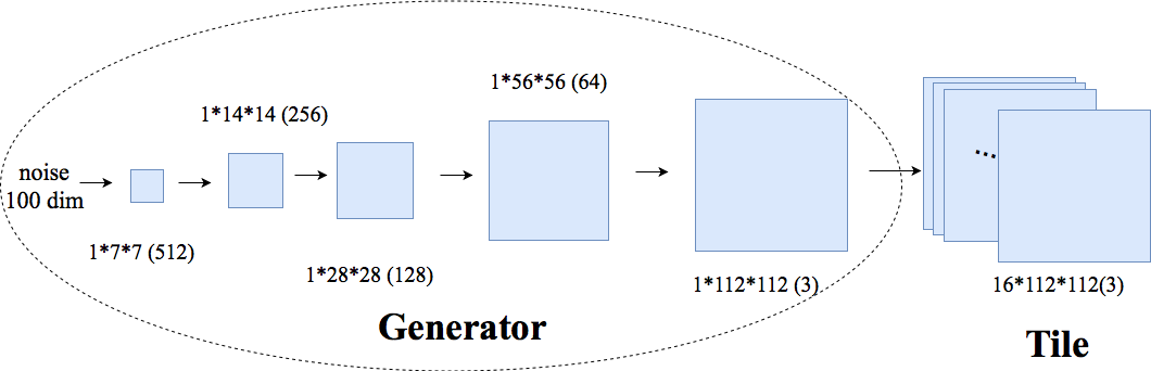
Figure 9. This figure illustrates the Generator and Tile for generating 2D-DUP. 1) The generator takes a noise vector as input, and outputs a single-frame perturbation. 2) The tile part constructs a perturbation clip by repeating the single-frame perturbation generated 16 times.

6.2. Circular Dual-Purpose Universal Perturbation

The above discussion shows that the boundary effect makes it especially challenging to attack video classification systems. To cope with this effect, we significantly extend the DUPs proposed in § 5 to compose what we call “Circular Dual-Purpose Universal Perturbations (C-DUP).”

Let us uppose that the size of sliding window is $w$. Then, the DUP clip $p$ includes $w$ frames (of perturbation), denoted by $[p_{1},p_{2},\cdots,p_{w}]$. Since $p$ is a clip of universal perturbations, we launch the attack by repeatedly adding perturbations on each consecutive clip consisting of $w$ frames, in the video stream. One can visualize that we are generating a perturbation stream which can be represented as $[\cdots,p_{w-1},p_{w},p_{1},p_{2},\cdots]$. Now, our goal is to guarantee that the perturbation stream works regardless of the clip boundaries chosen by the classifier. In order to achieve this goal, we need any cyclic or circular shift of the DUP clip to yield a valid perturbation. In other words, we require the perturbation clips $[p_{w},p_{1},\cdots,p_{w-1}]$, $[p_{w-1},p_{w},p_{1},\cdots,p_{w-2}]$, and so on, all to be valid perturbations. To formalize, we define a permutation function $Roll(p,o)$ which yields a cyclic shift of the original DUP perturbation by an offset $o$. In other words, when using $[p_{1},p_{2},\cdots,p_{w}]$ as input to $Roll(p,o)$, the output is $[p_{w-o},p_{w-o+1},\cdots p_{w},p{1}\cdots p_{w-o-1}]$. Now, for all values of $o\in\{0,w-1\}$, we need $p_{o}=Roll(p,o)$ to be a valid perturbation clip as well. Towards achieving this requirement, we use a post-processor unit which applies the roll function between the generator and the discriminator. This post processor is captured in the complete architecture is shown in 3(b).

The details of how the generator and the roll unit operate in conjunction are depicted in Figure 8. As before, the 3D generator ($G$) takes a noise vector as input and outputs a sequence of perturbations (as a perturbation clip). Note that the final layer is followed by a $tanh$ non-linearity which constrains the perturbation generated to the range [-1,1]. The last thing is to scale the output by $\xi$. Doing so restricts the perturbation’s range to $[-\xi,\xi]$. Following the work in (Moosavi-Dezfooli et al., 2017; Mopuri et al., 2017b), the value of $\xi$ is chosen to be 10 towards making the perturbation quasi-imperceptible. The roll unit then “rolls” (cyclically shifts) the perturbation $p$ by an offset in $\{0,1,2,\cdots,w-1\}$. Figure 8 depicts the process with an offset equal to 1; the black frame is rolled to the end of the clip. By adding the rolled perturbation clip to the training input, we get the perturbed input. As discussed earlier, the C3D classifier takes the perturbed input and outputs a classification score vector. As before, we want the true class scores to be (a) low for the targeted inputs and (b) high for other (non-targeted) inputs. We now modify our optimization function to incorporate the roll function as follows.

(3) $$\underset{G}{\text{minimize}}\quad\sum_{o=1,2\cdots w}\{\lambda\times\sum_{x_{t}\in T}{-\log[1-Q_{c(x_{t})}(x_{t}+Roll(G(z),o))]}$$

$$+\sum_{x_{s}\in S}{-\log[Q_{c(x_{s})}(x_{s}+Roll(G(z),o))]}\}$$

The equation is essentially the same as Equation 2, but we consider all possible cyclic shifts of the perturbation output by the generator.

6.3. 2D Dual-Purpose Universal Perturbation

We also consider a special case of C-DUP, wherein we impose an additional constraint which is that “the perturbations added on all frames should be the same.” In other words, we seek to add a single 2D perturbation on each frame which can be seen as a special case of C-DUP with $p_{1}=p_{2}=\cdots=p_{w}$. We call this kind of DUP as 2D-DUP. 2D-DUP allows us to examine the effect of the temporal dimension in generating adversarial perturbations on video inputs.

The generator in this case will output a single-frame perturbation instead of a sequence of perturbation frames as shown in Figure 9. This is a stronger constraint than the circular constraint, which may cause the attack success rate to decrease (note that the cyclic property still holds). However, with this constraint, the perturbation generated is much simpler and easier to use.

We denote the above 2D perturbation as $p_{2d}$. The perturbation clip is then generated by simply creating copies of the perturbation and tiling them to compose a clip. The 2D-DUP clip is now $p_{tile}=[p_{2d},p_{2d},\cdots,p_{2d}]$ (see Figure 9). Thus, given that the attack objective is the same as before, we simply replace the $Roll(p,o)$ function with a $Tile$ function and our formulation now becomes:

(4) $$\underset{G_{2D}}{\text{minimize}}\quad\lambda\times\sum_{x_{t}\in T}{-log[1-Q_{c(x_{t})}(x_{t}+Tile(G_{2D}(z)))]}$$

$$+\sum_{x_{s}\in S}{-log[Q_{c(x_{s})}(x_{s}+Tile(G_{2D}(z)))]}$$

7. Evaluations

In this section, we showcase the efficacy of the perturbations generated by our proposed approaches on both the UCF-101 and Jester datasets.

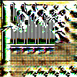
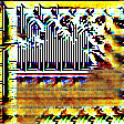
Figure 10. DUP on UCF-101

Figure 11. C-DUP on UCF-101

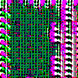
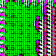
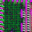
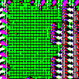
Figure 12. C-DUP on Jester for $T_{1}=\{\text{slding hand right}\}$

Figure 13. C-DUP on Jester for $T_{2}=\{\text{shaking hand}\}$

7.1. Experimental Setup

Discriminator set-up for our experiments: We used the C3D classifier as our discriminator. To set up the discriminator for our experiments, we pre-train the C3D classifier as described in §4. The discriminator is then used to train our generator. For our experiments on the UCF101 dataset, we use the C3D model available in the Github repository (Tensorflow, 2016). This pre-trained C3D model achieves an average clip classification accuracy of $96.1\%$ on the UCF101 dataset in benign settings (i.e., no adversarial inputs).

For the experiments on the Jester dataset, we fine-tune the C3D model from the Github repository (Tensorflow, 2016). First, we change the output size of the last fully connected layer to 27, since there are 27 gesture classes in Jester. We use a learning rate with exponential decay (Zeiler, 2012) to train the model. The starting learning rate for the last fully connected layer is set to be $10^{-3}$ and $10^{-4}$ for all the other layers. The decay step is set to 600 and the decay rate is 0.9. The fine-tuning phase is completed in 3 epochs and we achieve a clip classification accuracy of $90.03\%$ in benign settings.

Generator set-up for our experiments: For building our generators, we refer to the generative model used by Vondrik et al. (Vondrick et al., 2016), which has 3D de-convolution layers.

For generators for both C-DUP and 2D-DUP, we use five 3D de-convolution layers (Biggs, 2010). The first four layers are followed by a batch normalization (Ioffe and Szegedy, 2015) and a $ReLU$ (Nair and Hinton, 2010) activation function. The last layer is followed by a $tanh$ (Kalman and Kwasny, 1992) layer. The kernel size for all 3D de-convolutions is set to be $3\times 3\times 3$. To generate 3D perturbations (i.e., sequence of perturbation frames), we set the kernel stride in the C-DUP generator to 1 in both the spatial and temporal dimensions for the first layer, and 2 in both the spatial and temporal dimensions for the following 4 layers. To generate a single-frame 2D perturbation, the kernel stride in the temporal dimension is set to 1 (i.e., 2D deconvolution) for all layers in the 2D-CUP generator, and the spatial dimension stride is 1 for the first layer and 2 for the following layers. The numbers of filters are shown in brackets in Figure 8 and Figure 9. The input noise vector for both generators are sampled from a uniform distribution $U[-1,1]$ and the dimension of the noise vector is set to be 100. For training both generators, we use a learning rate with exponential decay. The starting learning rate is 0.002. The decay step is 2000 and the decay rate is 0.95. Unless otherwise specified, the weight balancing the two objectives, i.e., $\lambda$, is set to 1 to reflect equal importance between misclassifying the target class and retaining the correct classification for all the other (non-target) classes.

Technical Implementation: All the models are implemented in TensorFlow (Abadi et al., 2016) with the Adam optimizer (Kingma and Ba, 2014). Training was performed on 16 Tesla K80 GPU cards with the batch size set to 32.

Dataset setup for our experiments: On the UCF-101 dataset (denoted UCF-101 for short), different sets of target class $T$ are tested. We use $T=\{\text{apply lipstick}\}$ for presenting the results in the paper. Experiments using other target sets also yield similar results. UCF-101 has 101 classes of human actions in total. The target set $T$ contains only one class while the “non-target” set $S=X-T$ contains 100 classes. The number of training inputs from the non-target classes is approximately 100 times the number of training inputs from the target class. Directly training with UCF-101 may cause a problem due to the imbalance in the datasets containing the target and non-target classes (Longadge and Dongre, 2013). Therefore, we under-sample the non-target classes by a factor of 10. Further, when loading a batch of inputs for training, we fetch half the batch of inputs from the target set and the other half from the non-target set in order to balance the inputs.

For the Jester dataset, we also choose different sets of target classes. We use two target sets $T_{1}=\{\text{sliding hand right}\}$ and $T_{2}=\{\text{shaking hands}\}$ as our representative examples because they are exemplars of two different scenarios. Since we seek to showcase an attack on a video classification system, we care about how the perturbations affect both the appearance information and temporal flow information, especially the latter. For instance, the ‘sliding hand right’ class has a temporally similar class ‘sliding two fingers right;’ as a consequence, it may be easier for attackers to cause clips in the former class to be misclassified as the later class (because the temporal information does not need to be perturbed much). On the other hand, ‘shaking hands’ is not temporally similar to any other class. Comparing the results of these two target sets could provide some empirical evidence on the impact of the temporal flow on our perturbations. Similar to UCF-101, the number of inputs from the non-target classes is around 26 times the number of inputs from the target class (since there are 27 classes in total and we only have one target class in each experiment). So we under-sample the non-target inputs by a factor of 4. We also set up the environment to load half of the inputs from the target set and the other half from the non-target set, in every batch.

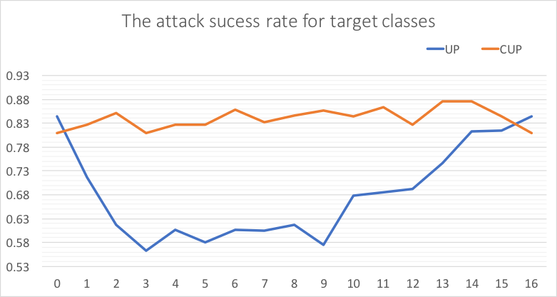
(a) Attack success rate on UCF-101 for target class
’applying lipstick’

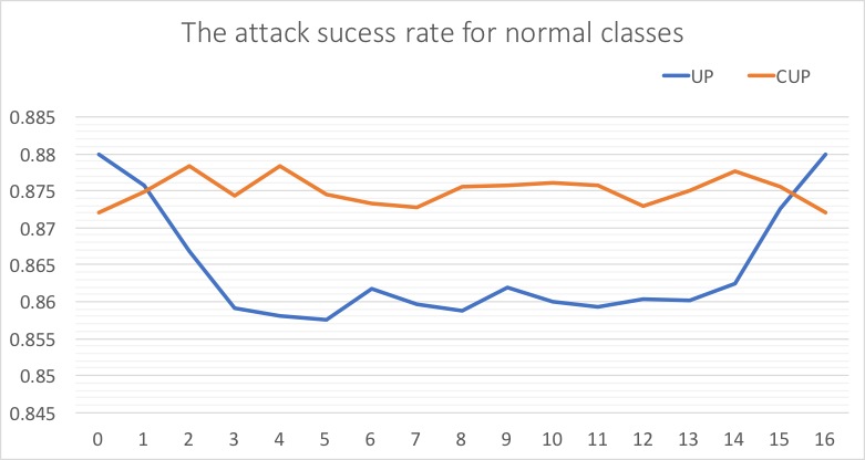
(b) Attack success rate on UCF-101 for other non-target classes (all except ’applying lipstick’)

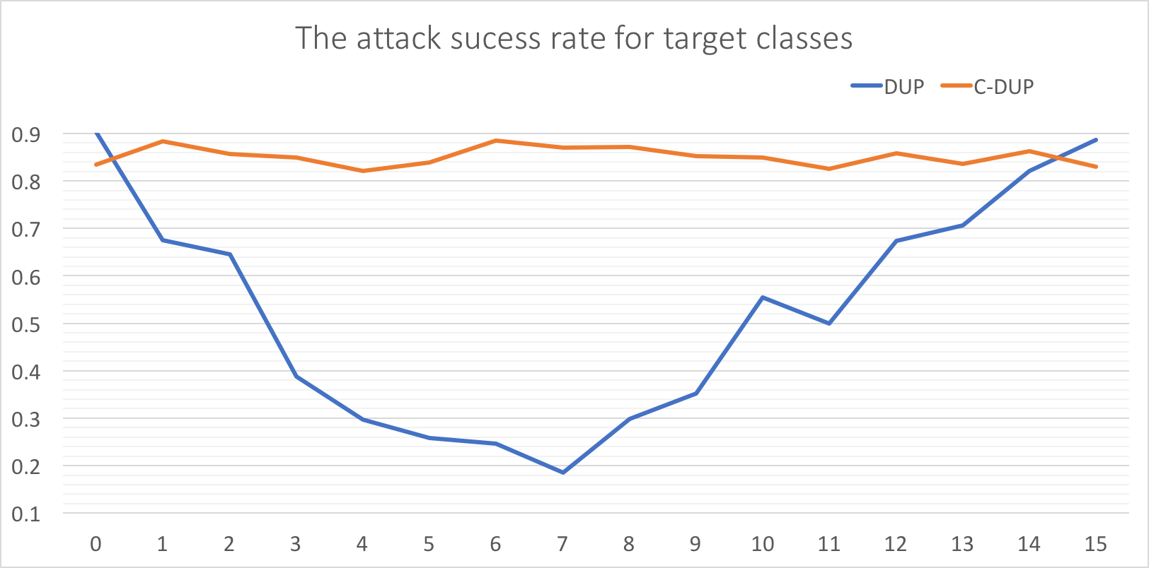
(c) Attack success rate on Jester for target class
’sliding hands right’

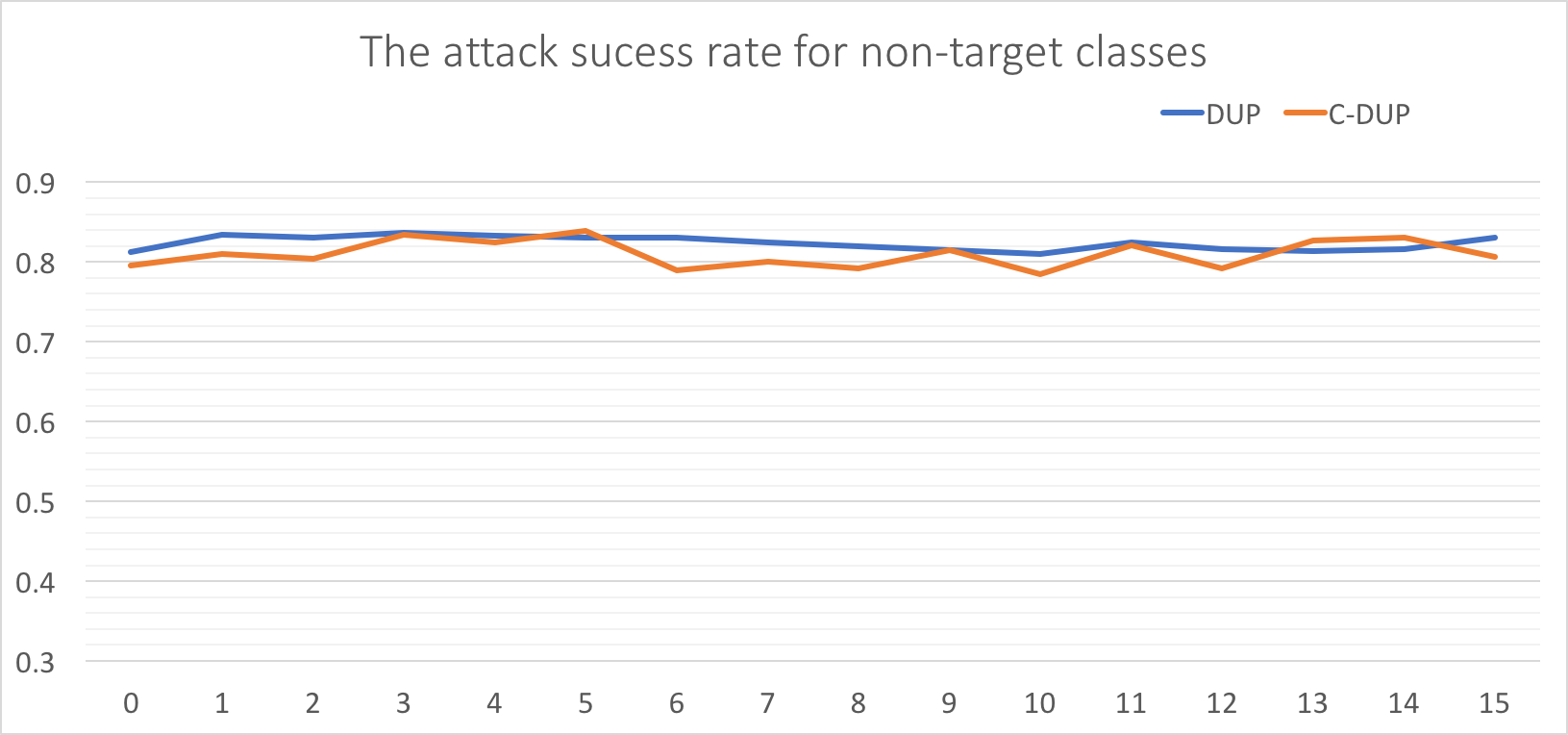
(d) Attack success rate on Jester for non-target classes (all excepet ’sliding right’)

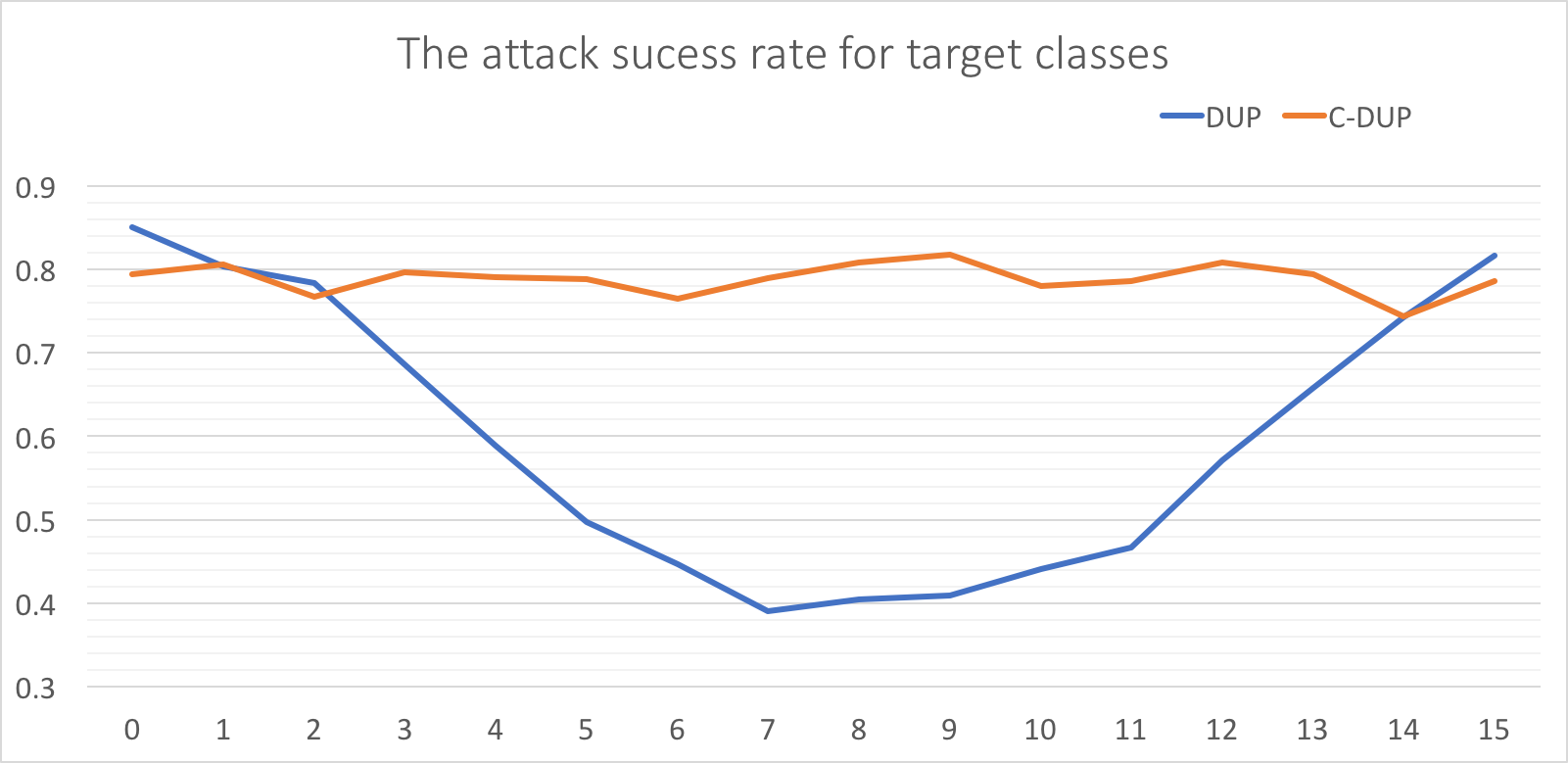
(e) Attack success rate on Jester for target class
’shaking hand’

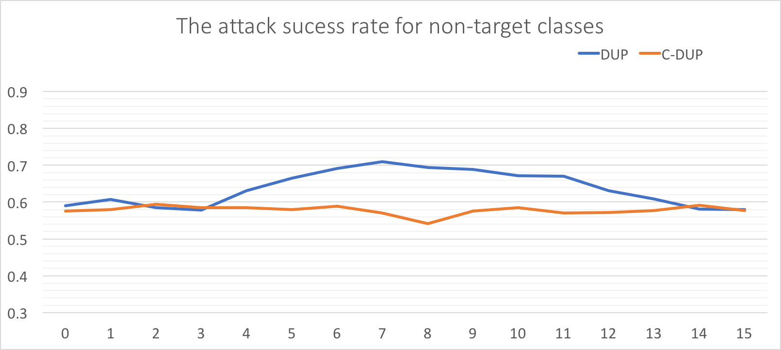
(f) Attack success rate on Jester for non-target classes (all except ’shaking hand’)

Figure 14. attack success rate for DUP and C-DUP

Metrics of interest: For measuring the efficacy of our perturbations, we consider two metrics. First, the perturbations added on the videos should be quasi-imperceptible. Second, the attack success rate for the target and the non-target classes should be high. We define attack success rates as follows:

• The attack success rate for the target class is the misclassification rate;

• the attack success rate for the other classes is the correct classification rate.

7.2. C-DUP Perturbations

In this subsection, we discuss the results of the C-DUP perturbation attack. We use the universal perturbations (UP) and DUP perturbations as our baselines.

7.2.1. Experimental Results on UCF101

Visualizing the perturbation: The perturbation clip generated by the DUP model is shown in Figure 10 and the perturbation clip generated by C-DUP model is shown in Figure 11. The perturbation clip has 16 frames, and we represent a visual representation of the first 8 frames for illustration We observe that the perturbation from DUP manifests an obvious disturbance among the frames. With C-DUP, the perturbation frames look similar, which implies that C-DUP does not perturb the temporal information by much, in UCF101.

Attack success rates: Recalling the discussion in §5, one can expect that UP would cause inputs from the target class to be misclassified, but also significantly affect the correct classification of the other non-target inputs. On the other hand, oue would expect that DUP would achieve a stealthy attack, which would not cause much effect on the classification of non-target classes.

Based on the discussion in §6, we expect that DUP would work well when the perturbation clip is well-aligned with the start point of each input clip to the classifier; and the attack success rate would degrade as the misalignment increases. We expect C-DUP would overcome this boundary effect and provide a better overall attack performance (even with temporal misalignment).

We observe that when one considers no misalignment, DUP achieves a target misclassification rate of 84.49 %, while the non-target classes are correctly classified with a rate of 88.03 %. In contrast, when UP achieves a misclassification rate of 84.01 % for the target class, only 45.2 % of the other classes are correctly classified. Given UP’s inferior performance, we do not consider it any further in our evaluations.

The attack success rates with DUP and C-DUP, on the UCF-101 test set, are shown in 14(a) and 14(b). The $x$ axis is the misalignment between perturbation clip and and the input clip to the classifier. 14(a) depicts the average misclassification rate for inputs from the target class. We observe that when there is no misalignment, the attack success rate with the DUP is $84.49\%$, which is in fact slightly higher than C-DUP. However, the attack success rate with C-DUP is significantly higher when there is misalignment. Furthermore, the average attack success rate across all alignments for the target class with C-DUP is $84\%$, while with DUP it is only $68.26\%$. This demonstrates that C-DUP is more robust against boundary effects.

14(b) shows that, with regards to the classification of inputs from the non-target classes, C-DUP also achieves a performance slightly better than DUP when there is mismatch. The average attack success rate (across all alignments) with C-DUP is $87.52\%$ here, while with DUP it is $84.19\%$.

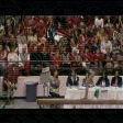
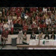
Figure 15. Visualizing images after adding 2D dual purpose universal perturbation: Original frames are displayed in the first row and perturbed frames are displayed in the second row. The perturbation added to the frames in the second row is mostly imperceptible to the human eye.

7.2.2. Experimental Results on Jester

Visualizing the perturbation: Visual representations of the C-DUP perturbations for the two target sets, $T_{1}=\{\text{sliding hand right}\}$ and $T_{2}=\{\text{shaking hands}\}$ are shown in Figure 12 and Figure 13. We notice that compared to the perturbation generated on UCF-101 (see Figure 11). there is a more pronounced evolution with respect to Jester (see Figure 12 and Figure 13). We conjecture that this is because UCF-101 is a coarse-grained action dataset in which the spatial (appearance) information is dominant. As a consequence, the C3D model does not extract/need much temporal information to perform well. However, Jester is a fine-grained action dataset where temporal information plays a more important role. Therefore, in line with expectations, we find that in order to attack the C3D model trained on the Jester dataset, a higher extent of perturbations are required on the temporal dimension.

Attack success rate: To showcase a comparison of the misclassification rates with respect to the target class between the two schemes (DUP and C-DUP), we adjust the weighting factor $\lambda$ such that the classification accuracy with respect to non-target classes are similar. By choosing $\lambda$ = 1.5 for DUP and 1 for C-DUP, we are able to achieve this. The attack success rates for the above two target sets are shown in 14(c) and 14(d), and 14(e) and 14(f), respectively. We see that with respect to $T_{1}=\{\text{sliding hand right}\}$, the results are similar to what we observe with UCF101. The attack success rates for C-DUP are a little lower than DUP when the offset is 0. This is to be expected since DUP is tailored for this specific offset. However, C-DUP outperforms DUP when there is a misalignment. The average success rate for C-DUP is $85.14\%$ for the target class and $81.03\%$ for the other (non-target) classes. The average success rate for DUP is $52.42\%$ for the target class and $82.36\%$ for the other (non-target) classes.

Next we consider the case with $T_{2}=\{\text{shaking hands}\}$. In general, we find that both DUP and C-DUP achieve relatively lower success rates especially with regards to the other (non-target) classes. As discussed in §7.1, unlike in the previous case where ‘sliding two fingers right’ is temporally similar to ‘sliding hand right’, no other class is temporally similar to ‘shaking hand’. Therefore it is harder to achieve misclassification. 14(f) depicts the attack success rates for non-target classes. The average success rate for non-target classes are similar (because of the bias in $\lambda$ as discussed earlier) and in fact slightly higher for DUP (a finer bias could make them exactly the same). The attack success rates with the two approaches for the target class are shown in 14(e). We see that C-DUP significantly outperforms DUP in terms of misclassification efficacy because of its robustness to temporal misalignment. The average attack success rate for the target class with C-DUP is $79.03\%$ while for DUP it is only $57.78\%$. Overall, our C-DUP outperforms DUP in being able to achieve a better misclassification rate for the target class. We believe that although stealth is affected to some extent, it is still reasonably high.

7.3. 2D-Dual Purpose Universal Perturbations

The visual representations of the perturbations with C-DUP show that perturbations on all the frames are visually similar. Thus, we ask if it is possible to add “the same perturbation” on every frame and still achieve a successful attack. In other words, will the 2D-DUP perturbation attack yield performance similar to the C-DUP attack.

7.3.1. Experimental Results on the UCF101 Dataset

Visual impact of the perturbation: We present a sequence of original frames and its corresponding perturbed frames in Figure 15. Original frames are displayed in the first row and perturbed frames are displayed in the second row. We observe that the perturbation added on the frames is quasi-imperceptible to human eyes (similar results are seen with C-DUP and are presented in an appendix).

Attack success rate: By adding 2D-DUP on the video clip, we achieve an attack success rate of $87.58\%$ with respect to the target class and an attack success rate of $83.37\%$ for the non-target classes. Recall that the average attack success rates with C-DUP were $87.52\%$ and $84.00\%$, respectively. Thus, the performance of 2D-DUP seems to be on par with that of C-DUP on the UCF101 dataset. This demonstrates that C3D is vulnerable even if the same 2D perturbation generated by our approach is added on to every frame.

7.3.2. Experimental Results on Jester Dataset

Attack success rate: For $T_{1}=\{\text{sliding hand right}\}$, the attack success rate for the target class is $84.64\%$ and the attack success rate for the non-target classes is $80.04\%$. This shows that 2D-DUP is also successful on some target classes in the fine-grained, Jester action dataset.

For the target set $T_{2}$, the success rate for the target class drops to $70.92\%$, while the success rate for non-target class is $54.83\%$. This is slightly degraded compared to the success rates achieved with C-DUP ($79.03\%$ and $57.78\%$ respectively), but is still reasonable. This degradation is due to more significant temporal changes in this case (unlike in the case of $T_{1}$) and a single 2D perturbation is less effective in manipulating these changes. In contrast, because the perturbations evolve with C-DUP, they are much more effective in achieving the misclassification of the target class.

8. Discussion

Black box attacks: In this work we assumed that the adversary is fully aware of the DNN being deployed (i.e., white box attacks). However, in practice the adversary may need to determine the type of DNN being used in the video classification system, and so a black box approach may be needed. Given recent studies on the transferability of adversarial inputs (Papernot et al., 2016b), we believe black box attacks are also feasible. We will explore this in our future work.

Context dependency: Second, the approach that we developed does not account for contextual information, i.e., consistency between the misclassified result and the context. For example, the context relates to a baseball game a human overseeing the system may notice an inconsistency when the action of hitting a ball is misclassified into applying makeup. Similarly, because of context, if there is a series of actions that we want to misclassify, inconsistency in the misclassification results (e.g., different actions across the clips) may also raise an alarm. For example, let us consider a case where the actions include running, kicking a ball, and applying make up. While the first two actions can be considered to be reasonable with regards to appearing together in a video, the latter two are unlikely. Generating perturbations that are consistent with the context of the video is a line of future work that we will explore and is likely to require new techniques. In fact, looking for consistency in context may be a potential defense, and we will also examine this in depth in the future.

Defenses: In order to defense against the attacks against video classification systems, one can try some existing defense methods in image area, such as feature squeezing (Xu et al., 2017b, a) and ensemble adversarial training (Tramèr et al., 2017) (although their effectiveness is yet unknown). Considering the properties of video that were discussed, we envision some exclusive defense methods for protecting video classification systems below, which we will explore in future work.

One approach is to examine the consistency between the classification of consecutive frames (considered as images) within a clip, and between consecutive clips in a stream. A sudden change in the classification results could raise an alarm. However, while this defense will work well in cases where the temporal flow is not pronounced (e.g., the UCF101 dataset), it may not work well in cases with pronounced temporal flows. For example, with respect to the Jester dataset, with just an image it may be hard to determine whether the hand is being moved right or left.

The second line of defense may be to identify an object that is present in the video, e.g., a soccer ball in a video clip that depicts a kicking action. We can use an additional classifier to identify such objects in the individual frames that compose the video. Then, we can look for consistency with regards to the action and the object, e.g., a kicking action is can be associated with a soccer ball, but cannot be associated with a make up kit. Towards realizing this line of defense, we could use existing image classifiers in conjunction with the video classification system. We will explore this in future work.

9. Related Work

There is quite a bit of work (Biggio et al., 2013; Biggio et al., 2014; Huang et al., 2011) on investigating the vulnerability of machine learning systems to adversarial inputs. Researchers have shown that generally, small magnitude perturbations added to input samples, change the predictions made by machine learning models. Most efforts, however, do not consider real-time temporally varying inputs such as video. Unlike these efforts, our study is focused on the generation of adversarial perturbations to fool DNN based real-time video action recognition systems.

The threat of adversarial samples to deep-learning systems has also received considerable attention recently. There are several papers in the literature (e.g., (Moosavi-Dezfooli et al., 2017; Moosavi Dezfooli et al., 2016; Sharif et al., 2016; Goodfellow et al., 2014a, b)) that have shown that the state-of-the-art DNN based learning systems are also vulnerable to well-designed adversarial perturbations (Szegedy et al., 2013). Szegedy et al. show that the addition of hardly perceptible perturbation on an image, can cause a neural network to misclassify the image. Goodfellow et al. (Goodfellow et al., 2014b) analyze the potency of adversarial samples available in the physical world, in terms of fooling neural networks. Moosavi-Dezfooli et al. (Moosavi-Dezfooli et al., 2017; Moosavi Dezfooli et al., 2016; Mopuri et al., 2017a) make a significant contribution by generating image-agnostic perturbations, which they call universal adversarial perturbations. These perturbations can cause all natural images belonging to target classes to be misclassified with high probability.

GANs or generative adversarial networks have been employed by Goodfellow et al. (Goodfellow et al., 2014a) and Radford et al. (Radford et al., 2015) in generating natural images. Mopuri et al. (Mopuri et al., 2017b) extend a GAN architecture to train a generator to model universal perturbations for images. Their objective was to explore the space of the distribution of universal adversarial perturbations in the image space. We significantly extend the generative framework introduced by Mopuri et al. (Mopuri et al., 2017b). In addition, unlike their work which focused on generating adversarial perturbations for images, our study focuses on the generation of effective perturbations to attack videos.

The feasibility of adversarial attacks against other types of learning systems including face-recognition systems (Sharif et al., 2016; McCoyd and Wagner, 2016; Sharif et al., 2017), voice recognition systems (Carlini et al., 2016) and malware classification systems (Grosse et al., 2016) has been studied. However, these studies do not account for the unique input characteristics that are present in real-time video activity recognition systems.

10. Conclusions

In this paper, we investigate the problem of generating adversarial samples for attacking video classification systems. We identify three key challenges that will need to be addressed in order to generate such samples namely, generating perturbations in real-time, making the perturbations stealthy and accounting for the temporal structure of frames in a video clip. We exploit recent advances in GAN architectures, extending them significantly to solve these challenges and generate very potent adversarial samples against video classification systems. We perform extensive experiments on two different datasets one of which captures coarse-grained actions (e.g., applying make up) while the other captures fine-grained actions (hand gestures). We demonstrate that our approaches are extremely potent, achieving around 80 % attack success rates in both cases. We also discuss possible defenses that we propose to investigate in future work.

Appendix A Appendix: Visualizing perturbations on UCF101

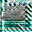
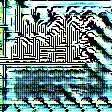
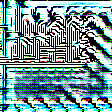
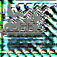
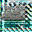
Figure 16. Circular Dual-Purpose Universal Perturbation (C-DUP) for UCF101

We visualize a full range of perturbations and their corresponding video representations on the UCF-101 dataset here. Figure 16 shows the entire Circular Dual-Purpose Universal Perturbation (C-DUP) clip (with 16 frames) generated for a target class $T=\{\text{apply lipstick}\}$. Similarly, Figure 17 shows the entire 2D Dual-Purpose Universal Perturbation (2D-DUP) for same target class.

Figure 18 shows a clean video clip from UCF101 dataset. Figure 19 shows the same video clip perturbed by the C-DUP shown in Figure 16. Similarly, Figure 20 shows the video clip perturbed by 2D-DUP shown in Figure 17. In both cases, we observe that the perturbation is quasi-imperceptible to human vision i.e., the frames in the videos look very much like the original.

Figure 17. 2D Dual-Purpose Universal Perturbation for UCF-101

Figure 18. Original frames from UCF-101

Figure 19. C-DUP perturbed frames from UCF-101

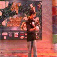
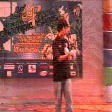
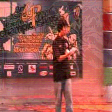
Figure 20. 2D-DUP perturbed frames from UCF-101

Appendix B Appendix: Visualizing perturbations on Jester

Figure 21 shows the entire C-DUP generated for clip to misclassify the target class $T=\{\text{shaking hand}\}$ on the Jester dataset. Similarly, Figure 22 depicts the entire 2D-DUP generated for misclassifying the same target class.

Figure 23 shows a clean video clip from Jester dataset corresponding to shaking of the hand (visible only in some of the frames shown due to cropping). Figure 24 shows the clip perturbed by C-DUP shown in Figure 21 from the Jester dataset. Similarly Figure 25 shows the same clip perturbed by 2D-DUP shown in Figure 22. It is easy to see that the perturbation is quasi-imperceptible to human vision.

Figure 21. C-DUP for Jester

Figure 22. 2D-DUP for Jester

Figure 23. Original frames from Jester

Figure 24. C-DUP perturbed frames from Jester

Figure 25. 2D-DUP perturbed frames from Jester

References

- (1)
- Abadi et al. (2016) Martín Abadi, Paul Barham, Jianmin Chen, Zhifeng Chen, Andy Davis, Jeffrey Dean, Matthieu Devin, Sanjay Ghemawat, Geoffrey Irving, Michael Isard, et al. 2016. TensorFlow: A System for Large-Scale Machine Learning.. In OSDI, Vol. 16. 265–283.
- Biggio et al. (2013) Battista Biggio, Igino Corona, Davide Maiorca, Blaine Nelson, Nedim Šrndić, Pavel Laskov, Giorgio Giacinto, and Fabio Roli. 2013. Evasion attacks against machine learning at test time. In Joint European conference on machine learning and knowledge discovery in databases. Springer, 387–402.
- Biggio et al. (2014) Battista Biggio, Giorgio Fumera, and Fabio Roli. 2014. Pattern recognition systems under attack: Design issues and research challenges. International Journal of Pattern Recognition and Artificial Intelligence 28, 07 (2014), 1460002.
- Biggs (2010) David SC Biggs. 2010. 3D deconvolution microscopy. Current Protocols in Cytometry (2010), 12–19.
- Carlini et al. (2016) Nicholas Carlini, Pratyush Mishra, Tavish Vaidya, Yuankai Zhang, Micah Sherr, Clay Shields, David Wagner, and Wenchao Zhou. 2016. Hidden Voice Commands.. In USENIX Security Symposium. 513–530.
- Carreira and Zisserman (2017) Joao Carreira and Andrew Zisserman. 2017. Quo vadis, action recognition? a new model and the kinetics dataset. In 2017 IEEE Conference on Computer Vision and Pattern Recognition (CVPR). IEEE, 4724–4733.
- Dataset (2016) Jester Dataset. 2016. Humans performing pre-defined hand actions. https://20bn.com/datasets/jester. [Online; accessed 30-April-2018].
- Fanello et al. (2013) Sean Ryan Fanello, Ilaria Gori, Giorgio Metta, and Francesca Odone. 2013. One-shot learning for real-time action recognition. In Iberian Conference on Pattern Recognition and Image Analysis. Springer, 31–40.
- Foroughi et al. (2008) Homa Foroughi, Baharak Shakeri Aski, and Hamidreza Pourreza. 2008. Intelligent video surveillance for monitoring fall detection of elderly in home environments. In Computer and Information Technology, 2008. ICCIT 2008. 11th International Conference on. IEEE, 219–224.
- Goodfellow et al. (2014a) Ian Goodfellow, Jean Pouget-Abadie, Mehdi Mirza, Bing Xu, David Warde-Farley, Sherjil Ozair, Aaron Courville, and Yoshua Bengio. 2014a. Generative adversarial nets. In Advances in neural information processing systems. 2672–2680.
- Goodfellow et al. (2014b) Ian J Goodfellow, Jonathon Shlens, and Christian Szegedy. 2014b. Explaining and harnessing adversarial examples. arXiv preprint arXiv:1412.6572 (2014).
- Grosse et al. (2016) Kathrin Grosse, Nicolas Papernot, Praveen Manoharan, Michael Backes, and Patrick McDaniel. 2016. Adversarial perturbations against deep neural networks for malware classification. arXiv preprint arXiv:1606.04435 (2016).
- Gu et al. (2017) Jiuxiang Gu, Zhenhua Wang, Jason Kuen, Lianyang Ma, Amir Shahroudy, Bing Shuai, Ting Liu, Xingxing Wang, Gang Wang, Jianfei Cai, et al. 2017. Recent advances in convolutional neural networks. Pattern Recognition (2017).
- Herath et al. (2017) Samitha Herath, Mehrtash Harandi, and Fatih Porikli. 2017. Going deeper into action recognition: A survey. Image and vision computing 60 (2017), 4–21.
- Huang et al. (2011) Ling Huang, Anthony D Joseph, Blaine Nelson, Benjamin IP Rubinstein, and JD Tygar. 2011. Adversarial machine learning. In Proceedings of the 4th ACM workshop on Security and artificial intelligence. ACM, 43–58.
- Huang et al. (2017) Xun Huang, Yixuan Li, Omid Poursaeed, John Hopcroft, and Serge Belongie. 2017. Stacked generative adversarial networks. In IEEE Conference on Computer Vision and Pattern Recognition (CVPR), Vol. 2. 4.
- Ioffe and Szegedy (2015) Sergey Ioffe and Christian Szegedy. 2015. Batch normalization: Accelerating deep network training by reducing internal covariate shift. arXiv preprint arXiv:1502.03167 (2015).
- Kalman and Kwasny (1992) Barry L Kalman and Stan C Kwasny. 1992. Why tanh: choosing a sigmoidal function. In Neural Networks, 1992. IJCNN., International Joint Conference on, Vol. 4. IEEE, 578–581.
- Karpathy et al. (2014) Andrej Karpathy, George Toderici, Sanketh Shetty, Thomas Leung, Rahul Sukthankar, and Li Fei-Fei. 2014. Large-scale video classification with convolutional neural networks. In Proceedings of the IEEE conference on Computer Vision and Pattern Recognition. 1725–1732.
- Kataoka et al. (2018a) Hirokatsu Kataoka, Yutaka Satoh, Yoshimitsu Aoki, Shoko Oikawa, and Yasuhiro Matsui. 2018a. Temporal and fine-grained pedestrian action recognition on driving recorder database. Sensors 18, 2 (2018), 627.
- Kataoka et al. (2018b) Hirokatsu Kataoka, Teppei Suzuki, Shoko Oikawa, Yasuhiro Matsui, and Yutaka Satoh. 2018b. Drive Video Analysis for the Detection of Traffic Near-Miss Incidents. arXiv preprint arXiv:1804.02555 (2018).
- Kingma and Ba (2014) Diederik P Kingma and Jimmy Ba. 2014. Adam: A method for stochastic optimization. arXiv preprint arXiv:1412.6980 (2014).
- Lab (2014) Kaspersky Lab. Defcon,2014. Man-in-the-middle attack on video surveillance systems. https://securelist.com/does-cctv-put-the-public-at-risk-of-cyberattack/70008/. [Online; accessed 30-April-2018].
- Longadge and Dongre (2013) Rushi Longadge and Snehalata Dongre. 2013. Class imbalance problem in data mining review. arXiv preprint arXiv:1305.1707 (2013).
- McCoyd and Wagner (2016) Michael McCoyd and David Wagner. 2016. Spoofing 2D Face Detection: Machines See People Who Aren’t There. arXiv preprint arXiv:1608.02128 (2016).
- Moosavi-Dezfooli et al. (2017) Seyed-Mohsen Moosavi-Dezfooli, Alhussein Fawzi, Omar Fawzi, and Pascal Frossard. 2017. Universal Adversarial Perturbations. In Computer Vision and Pattern Recognition (CVPR), 2017 IEEE Conference on. IEEE, 86–94.
- Moosavi Dezfooli et al. (2016) Seyed Mohsen Moosavi Dezfooli, Alhussein Fawzi, and Pascal Frossard. 2016. Deepfool: a simple and accurate method to fool deep neural networks. In Proceedings of 2016 IEEE Conference on Computer Vision and Pattern Recognition (CVPR).
- Mopuri et al. (2017a) Konda Reddy Mopuri, Utsav Garg, and R Venkatesh Babu. 2017a. Fast Feature Fool: A data independent approach to universal adversarial perturbations. arXiv preprint arXiv:1707.05572 (2017).
- Mopuri et al. (2017b) Konda Reddy Mopuri, Utkarsh Ojha, Utsav Garg, and R Venkatesh Babu. 2017b. NAG: Network for Adversary Generation. arXiv preprint arXiv:1712.03390 (2017).
- Nair and Hinton (2010) Vinod Nair and Geoffrey E Hinton. 2010. Rectified linear units improve restricted boltzmann machines. In Proceedings of the 27th international conference on machine learning (ICML-10). 807–814.
- Net (2016) ZD Net. ZD Net,2016. Surveillance cameras sold on Amazon infected with malware. https://www.zdnet.com/article/amazon-surveillance-cameras-infected-with-malware/. [Online; accessed 30-April-2018].
- Papernot et al. (2016a) Nicolas Papernot, Nicholas Carlini, Ian Goodfellow, Reuben Feinman, Fartash Faghri, Alexander Matyasko, Karen Hambardzumyan, Yi-Lin Juang, Alexey Kurakin, Ryan Sheatsley, et al. 2016a. cleverhans v2. 0.0: an adversarial machine learning library. arXiv preprint arXiv:1610.00768 (2016).
- Papernot et al. (2016b) Nicolas Papernot, Patrick McDaniel, and Ian Goodfellow. 2016b. Transferability in machine learning: from phenomena to black-box attacks using adversarial samples. arXiv preprint arXiv:1605.07277 (2016).
- Radford et al. (2015) Alec Radford, Luke Metz, and Soumith Chintala. 2015. Unsupervised representation learning with deep convolutional generative adversarial networks. arXiv preprint arXiv:1511.06434 (2015).
- Sharif et al. (2016) Mahmood Sharif, Sruti Bhagavatula, Lujo Bauer, and Michael K Reiter. 2016. Accessorize to a crime: Real and stealthy attacks on state-of-the-art face recognition. In Proceedings of the 2016 ACM SIGSAC Conference on Computer and Communications Security. ACM, 1528–1540.
- Sharif et al. (2017) Mahmood Sharif, Sruti Bhagavatula, Lujo Bauer, and Michael K Reiter. 2017. Adversarial Generative Nets: Neural Network Attacks on State-of-the-Art Face Recognition. arXiv preprint arXiv:1801.00349 (2017).
- Soomro et al. (2012) Khurram Soomro, Amir Roshan Zamir, and Mubarak Shah. 2012. UCF101: A dataset of 101 human actions classes from videos in the wild. arXiv preprint arXiv:1212.0402 (2012).
- Sultani et al. (2018) Waqas Sultani, Chen Chen, and Mubarak Shah. 2018. Real-world Anomaly Detection in Surveillance Videos. arXiv preprint arXiv:1801.04264 (2018).
- Szegedy et al. (2013) Christian Szegedy, Wojciech Zaremba, Ilya Sutskever, Joan Bruna, Dumitru Erhan, Ian Goodfellow, and Rob Fergus. 2013. Intriguing properties of neural networks. arXiv preprint arXiv:1312.6199 (2013).
- Tensorflow (2016) C3D Tensorflow. 2016. C3D Implementation. https://github.com/hx173149/C3D-tensorflow.git. [Online; accessed 30-April-2018].
- Tramèr et al. (2017) Florian Tramèr, Alexey Kurakin, Nicolas Papernot, Dan Boneh, and Patrick McDaniel. 2017. Ensemble adversarial training: Attacks and defenses. arXiv preprint arXiv:1705.07204 (2017).
- Tran et al. (2015) Du Tran, Lubomir Bourdev, Rob Fergus, Lorenzo Torresani, and Manohar Paluri. 2015. Learning spatiotemporal features with 3d convolutional networks. In Computer Vision (ICCV), 2015 IEEE International Conference on. IEEE, 4489–4497.
- Tripathi et al. (2016) Vikas Tripathi, Ankush Mittal, Durgaprasad Gangodkar, and Vishnu Kanth. 2016. Real time security framework for detecting abnormal events at ATM installations. Journal of Real-Time Image Processing (2016), 1–11.
- Varol et al. (2017) Gul Varol, Ivan Laptev, and Cordelia Schmid. 2017. Long-term temporal convolutions for action recognition. IEEE transactions on pattern analysis and machine intelligence (2017).
- Vision ([n. d.]a) Umboo Computer Vision. [n. d.]a. Case Study: Elementary Scholl in Taiwai. https://news.umbocv.com/case-study-taiwan-elementary-school-13fa14cdb167.
- Vision ([n. d.]b) Umboo Computer Vision. [n. d.]b. Umbo Customer Case Study NCHU. https://news.umbocv.com/umbo-customer-case-study-nchu-687356292f43.
- Vision ([n. d.]c) Umboo Computer Vision. [n. d.]c. Umbo’s Smart City Featured on CBS Sacramento. https://news.umbocv.com/umbos-smart-city-featured-on-cbs-sacramento-26f839415c51.
- Vision (2016) Umboo Computer Vision. 2016. Case Studies. https://news.umbocv.com/case-studies/home. [Online; accessed 30-April-2018].
- Vondrick et al. (2016) Carl Vondrick, Hamed Pirsiavash, and Antonio Torralba. 2016. Generating videos with scene dynamics. In Advances In Neural Information Processing Systems. 613–621.
- Xu et al. (2017a) Weilin Xu, David Evans, and Yanjun Qi. 2017a. Feature squeezing: Detecting adversarial examples in deep neural networks. arXiv preprint arXiv:1704.01155 (2017).
- Xu et al. (2017b) Weilin Xu, David Evans, and Yanjun Qi. 2017b. Feature squeezing mitigates and detects carlini/wagner adversarial examples. arXiv preprint arXiv:1705.10686 (2017).
- Zeiler (2012) Matthew D Zeiler. 2012. ADADELTA: an adaptive learning rate method. arXiv preprint arXiv:1212.5701 (2012).
- Zhu et al. (2016) Jun-Yan Zhu, Philipp Krähenbühl, Eli Shechtman, and Alexei A Efros. 2016. Generative visual manipulation on the natural image manifold. In European Conference on Computer Vision. Springer, 597–613.