Evenly Cascaded Convolutional Networks

Abstract

We introduce Evenly Cascaded convolutional Network (ECN), a neural network taking inspiration from the cascade algorithm of wavelet analysis. ECN employs two feature streams - a low-level and high-level steam. At each layer these streams interact, such that low-level features are modulated using advanced perspectives from the high-level stream. ECN is evenly structured through resizing feature map dimensions by a consistent ratio, which removes the burden of ad-hoc specification of feature map dimensions. ECN produces easily interpretable features maps, a result whose intuition can be understood in the context of scale-space theory. We demonstrate that ECN’s design facilitates the training process through providing easily trainable shortcuts. We report new state-of-the-art results for small networks, without the need for additional treatment such as pruning or compression - a consequence of ECN’s simple structure and direct training. A 6-layered ECN design with under 500k parameters achieves 95.24% and 78.99% accuracy on CIFAR-10 and CIFAR-100 datasets, respectively, outperforming the current state-of-the-art on small parameter networks, and a 3 million parameter ECN produces results competitive to the state-of-the-art.

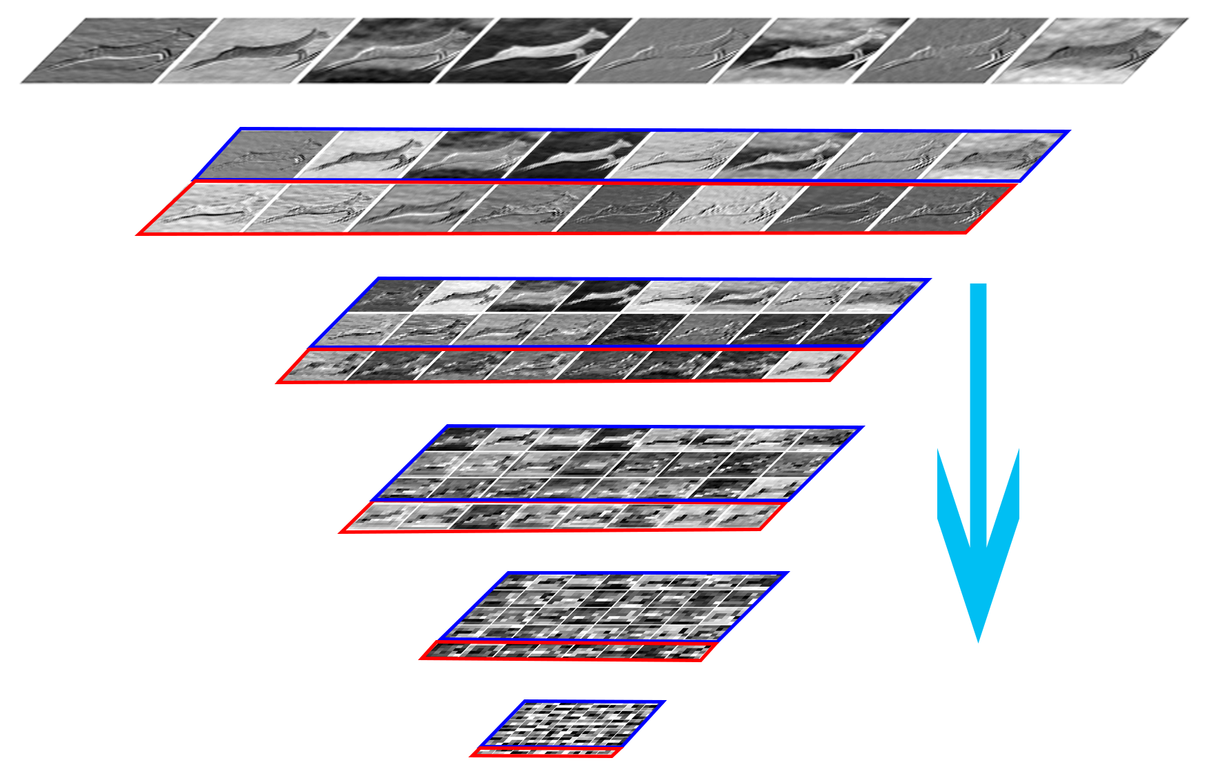
Figure 1: Our evenly cascaded design with $6$ cascading layers using a scaling rate of $0.75$. The growth rate (the number of high level feature channels generated in each subsequent layer) is set to $8$. From the second layer on, the low level feature channels are framed in blue boxes, the newly generated high level feature channels are framed in red boxes.

1 Introduction

How do humans come to understand their world? Consider the learning of mathematics - we learn basic mathematics before proceeding to advanced mathematics, the understanding of basic math serving as the foundation on which to develop an understanding of advanced math. Once an advanced understanding of math is acquired, it in turn is used to better understand basic math, reinforcing an understanding of mathematics as a whole. Similarly in perception - higher levels of abstraction within our perceptual hierarchies are built upon the lower levels of abstraction. Additionally, using higher level interpretations to reinforce lower level interpretations can provide benefits to perception as a whole, in the same way that using a more expansive understanding of mathematics to understand elementary mathematics reinforces an understanding of mathematics as a whole.

Disregarding the interplay between levels of abstraction in perception, the recent trend in deep neural networks is to simply make networks deeper. Since networks have become so deep, researchers have developed a now standard design that divides network layers into blocks of layers [22, 29, 10, 16]. Each block consists of layers of transforms that produce feature maps of the same shape. Cross-block transforms recombine the previous features and incorporate strided convolutions or pooling operations to reshape the feature maps. This strategy is an extension of the traditional design of the multilayer perceptron or fully-connected network [28]. The introduction of blocks has allowed a better organization of the evolving layers of abstraction within those networks. Overall, more high level features are abstracted through these transforms (Fig. 1, 3). However, the unstructured recombination of features in existing networks has made the investigation of deep neural networks nontrivial [34, 26].

Aside from deviating from basic intuitions about learning and perception, the now standard design has other apparent shortcomings. Since strided convolution or pooling are used to resize the feature maps by integer scales, researchers are compelled to create ad hoc network shapes, ones which are subject to awkward constraints of integer pooling and strides. Some networks assign more layers in later stages, where the feature maps are very small [10]. Some other networks are wider but have fewer layers [33]. The specification of feature map dimensions or distribution of computational resources is highly engineered and uneven in these designs. It is difficult to determine which designs outperform others, given that the overall shape is different. To make things worse, when the task changes, the network shape needs to be handcrafted again.

Arguably the biggest shortcoming of existing designs is that they afford little intuition on the training process, and consequently make deep networks notoriously hard to train. Researchers have expended significant effort in developing better methods to train these networks.

In this work we introduce an architecture more closely in line with intuitions of biological learning and perception: Evenly Cascaded convolutional Network (ECN). ECN is 1) easier than existing architectures to adapt to new tasks, 2) produces internal representations which are more humanly interpretable, 3) performs robustly as parameter count is restricted, and 4) produces competitive performance when compared to other state-of-the-art methods.

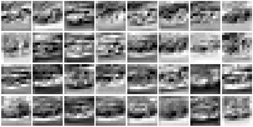
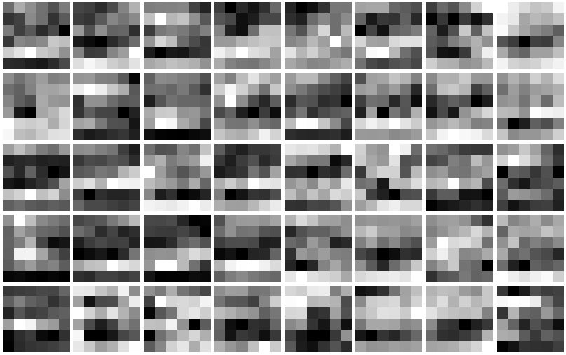
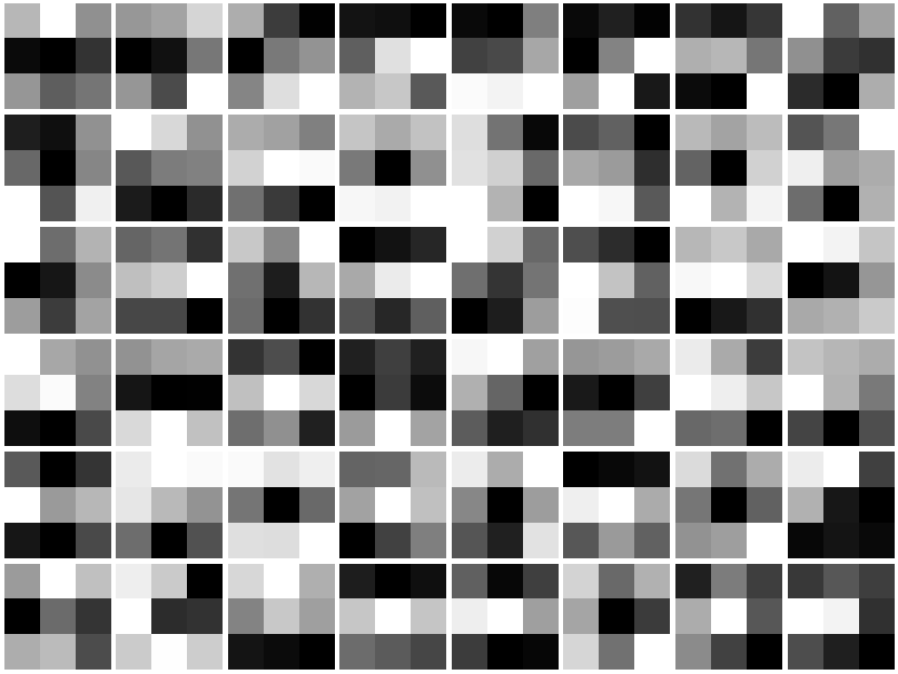
Figure 2: Visualizations of feature maps in ECN. The underlying network has $8$ feature maps in the first hidden layer. The feature channel growth rate is set to $8$. In this $6$-hidden-layer network there are $8,16,24,32,40,48$ feature maps in layers 1-6 respectively. In each deeper layer the newly generated higher level feature maps are appended as a new row. (a) Level 1 feature maps in the first hidden layer. (b) Level 1 features are adapted and tiled in the first row, level 2 features are newly generated using level 1 features, and are appended in the second row. (c) Both level 1 and level 2 features are adapted and tiled in the first two rows. Level 3 features are newly generated from level 1 and level 2 features, and are appended as the third row. (d) Level 4 features. (e) Level 5 features. (f) Level 6 features are used for recognition. The feature maps have been rescaled for better visualization.

ECN is structured around the insights that 1) maintaining low-level features through to the upper layers of a network is beneficial, 2) allowing multiple levels of features to interact with each other within the network is beneficial, 3) abrupt changes in feature map dimension could be less ideal than gradual changes, and 4) the manner in which features are conventionally combined within network blocks hampers the preservation of low-level features. Our architecture instantiates the first two of these insights through a “cascade” architecture - a two stream architecture, one stream for low-level features, one stream for successively higher level features, where these two streams interact at every layer. This differs from the existing method of using skip connections to introduce low-level features into upper level network layers in that low level features are maintained, and modulated appropriately, rather than simply jumping layers [16]. This approach differs from a conventional two-stream approach [4] in that both streams interact with each other. For the third insight, in both streams of our cascade architecture bilinear interpolation is employed for fractional pooling, allowing a gradual rather than abrupt decrease of feature map dimensions. Different from existing architectures, in ECN a scaling factor is introduced which simplifies the design of the shape of the network removing the need for handcrafting network shape. For the fourth insight we remove the conventional combination of features across blocks in neural networks in order to preserve the low-level signal in ECN’s two-stream cascade architecture. We demonstrate that preserving multilevel features enhances training by providing easy-to-train shortcuts.

Our evaluation of ECN resulted in several intriguing results: 1) With ECN’s principled structuring, shallow networks (Fig. 1) seem to perform competitively well when compared to extremely deep networks. 2) Complex high level tasks such as image classification can be approached through evenly downsampling and adapting a set of highly structured features (Fig. 2). 3) Low level features may be of critical importance in high level tasks such as image classification: not only do these features remain similar in the deeper adaptation process, but they may have provided major convenience for the training of high level features.

Finally, we evaluate ECN using multiple convolution block designs and find that recurrent and recursive designs lead to improved efficiency and accuracy. Without additional treatment, a standard convolution block design combined with recurrent connections leads to state-of-the-art accuracy in benchmark image classification tasks. Another block design using a recursive filter gives rise to state-of-the-art efficiency. Our 6-cascading-layer design with under 500k parameters achieves 95.24% and 78.99% accuracy on CIFAR-10 and CIFAR-100 datasets, respectively, outperforming the current state-of-the-art on small parameter networks, and our 3 million parameter version is competitive to the state-of-the-art.

2 Related Work

Even though convolutional networks have led to many exciting breakthroughs in visual and language learning tasks [22], the mathematical understanding of convolutional networks is severely underdeveloped. It is intuitively clear that convolutional networks can be understood in part within the context of scale-space theory or multiresolution analysis [27]. While an excellent attempt has been made [26] to explain convolutional networks in wavelet terms, it remains unclear how the techniques in wavelet theory can be explicitly used to simplify the construction and training of convolutional networks.

Skip connections or identity maps in the networks [13, 10, 16, 2] are a popular method for improving network performance. One intuitive understanding of the function of skip connections is that they pass lower level representations to deeper levels. In LSTM [13] and ResNet [10] networks the representations are adapted during this process. Whereas in DenseNet [16] shallow features are passed to the deeper levels without modification. One recent work, termed Dual Path Networks(DPN) [2], connects the two approaches using a high order recurrent neural network, and horizontally concatenates ResNet [10] and DensNet [16], and shows improved performance.

Presently, the best performing networks are typically 50 to 100 layers deep [10, 16, 31]. Translating an existing backbone architecture to a new application with different input and output sizes is a nontrivial task. The structuring of these standard designs are constrained by integer resizing operations such as pooling and strided convolution. Fractional pooling and strides have been explored previously, e.g. [8]. In our implementation of fractional pooling we employ bilinear interpolation, as is done in [20]. Furthermore, existing architectures merge different levels of features at the end of each block such that low- and high-level features become entangled and in-differentiable. ECN safely removes these limitations.

As the networks become wider and deeper, methods such as pruning [9, 23, 25], quantizing [5], and knowledge distillation [12] have been introduced to reduce the size of these networks. ECN uses recursion[24, 30] to re-use parameters across layers, allowing for greater compactness of network design. In the other direction, significant efforts have been spent on discovering more efficient network layers or overall architectures [18, 14, 36, 15, 16, 35].

3 Methods

ECN is based on a simple cascading layer design. Intuitively, a cascading layer incorporates multilevel features and gradually resizes those features before providing them to the next layer. ECN consists of iteratively stacked cascading layers. This iterative construction process ends when a stopping condition is met - e.g., when feature map dimensions fall below a predefined size.

3.1 Utilization of Multilevel Features

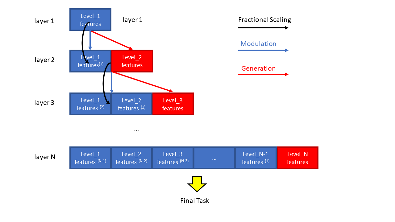
Figure 3: Multilevel feature representations within ECN. For the $i$-th layer ($i$-th row in the figure), fractional scaling is used to downsample the features from layer $i-1$ (row $i-1$ in the figure). A convolution block is applied over these downsampled features to generate the modulation signal, and the level $i$ features (red block). The modulation signal is then added to the features downsampled from the previous layer. The superscripts in each block represent the number of modulations the features have undergone.

We now follow the intuition that allowing an interplay between level of abstraction within perception can give rise to greater perceptual synergy at the beginning of Section 1 in introducing ECN’s usage of multilevel features. To illustrate ECN’s relation to work in the literature we also provide three additional viewpoints of our utilization of multilevel features: one from the network architecture, one from wavelet analysis, and one from optimization of neural networks.

3.1.1 From a Network Architectural Point of View

Our cascading design can be viewed as evolving from the designs of several well-performing networks [10, 16, 2]. Our first design can be viewed as a ResNet-inspired DenseNet, or a DenseNet-inspired ResNet. We make an extension to DenseNet [16] when passing low level features to deeper layers by allowing them to be modulated by higher level features. The modulation of low level features can be viewed as a feedback mechanism, where high level knowledge is providing “advanced viewpoints” to improve the low level knowledge, effected through a link from the higher level stream to the lower level stream of the network. The modulation signal is generated using a convolution block, and is added to the original features as in residual learning [10]. The generation of high level features is also achieved using the convolution block - however, the results are appended to the existing channels (Figs. 1, 3). Similar to our design, but more costly, Dual Path Network [2] concatenates ResNet and DenseNet layers. By not passing low-level features through a $1\times 1$ convolution, such as is done in DPN, ECN better preserves low-level features, making them more directly available at higher layers.

As a consequence of this ECN is able to pass features throughout the whole network, rather than only within each block. With this design we explicitly enforce that the shallowest level features be preserved throughout the whole network, with adaptations made only if they improve the final task (Figs. 1, 2).

3.1.2 From a Wavelet Point of View

It is noteworthy that the cascading layer is a more general form of the cascade algorithm used in wavelet packet decomposition [4, 27], where previous level signals are decomposed into a low frequency branch and a high frequency branch, usually followed by downsampling by a factor of $2$. In wavelet packet decomposition, the original signal is decomposed into a binary tree. The difference between this and ECN is that in ECN the two siblings are merged before the next level of decomposition, deviating from a tree structure. The extensions we made in our cascading design derive from the adaptations and downsampling of features which we introduce later. Due to the cascading design, the evolution of feature maps within ECN closely resembles the evolution of modulus maxima in scale-space theory [27]. This relation suggests a path for further mathematical investigation of neural networks.

3.1.3 From an Optimization Point of View

ECN’s construction facilitates training by providing easily trainable shortcuts to the optimization: we speculate that as a consequence of the two stream architecture, ECN allows the decomposition of $f$, the mapping from network input to output, into a series of progressively hierarchically deeper, and therefore harder to train, functions: $f=f_{1}+f_{2}+...+f_{N}$. See figure 3 for a visualization of function decomposition within and across layers. In figure 3 layer N contains features of levels $1$ through $N$ - this provides a direct link from the training (gradient) signal not only to higher level features, as is the case in other architectures, but to mid- and low-level features as well. This relaxes the interdependence in training between $f_{i}$ (low $f_{i}$ can be trained with less dependence on high $f_{i}$), and has the potential to facilitate training by allowing a training of $f$ component-wise. The result of this is the capability to train a complex function, $f$, by training the simpler functions of which it is composed, $f_{i}$.

Decompositions analogous to this kind have been proven to be helpful in multiscale signal analysis. Complex operations are simplified by conducting them at multiple scales, either (1) from coarse-to-fine or (2) in parallel. Here, we take the second approach to train different levels in parallel: the easier to train, or coarse, components can serve as a backbone model for the harder components, where the harder-to-train layers have only to compensate for the residuals of the learning problem. We conjecture that ECN’s construction facilitates the progressive training of neural networks. Note that ECN’s construction is a revival of the layer-wise pretraining technique [1] which triggered the era of deep learning. This classic approach followed the correct intuition of progressively developing high level representations. But the layer-wise training, which belongs to the first approach, lacks proper supervision signal.

3.2 Fractional Scaling

To facilitate the passing of low level features throughout the whole network, and to evenly resize the feature maps in a network, we propose to use fractional scaling, performed using bilinear interpolation, replacing the classic integer pooling and striding operations. Bilinear interpolation was first introduced in Spatial Transformer Networks [20] to continuously deform feature maps for recognition tasks. Here we use bilinear interpolation to replace all the size change operations in the network.

Using bilinear interpolation, the outputs of the previous layer are fractionally scaled to the desired shape, and then serve as inputs to the next layer. Since bilinear interpolation is a locally smooth operation, subgradients can be calculated for backpropagation. In a network with a decreasing feature map dimension, having a constant scaling factor close to $1$ leads to a deep network. Similarly, having a constant scaling factor close to $0$ leads to a shallow network.

We adopt a simple uniform sampling when scaling the feature maps for obtaining the sample grid for bilinear interpolation. Non-uniform sampling is a natural extension [6] and we leave it for future work. Here, the output feature map dimension can be either calculated from the scaling factor or manually specified. The uniformly spaced sampling grid is then calculated to sample from the previous feature map.

3.3 Convolution Block Design

Many researchers have proposed different convolution block designs for use within layers of convolutional networks. However, in most cases different block designs are associated with different network architectures. As a consequence, it is difficult to draw conclusions about the relative merits of different block designs. However, with ECN’s evenly cascaded design, it is straightforward to incorporate different block designs. In this work we propose and evaluate multiple block designs. More advanced block designs than are presented here can be evaluated in subsequent works and potentially result in improved performance. In this paper we include six basic blocks:

Block 1: Single convolution (Fig. 4(a)). The convolutional layer has one single convolution operation, combined with standard techniques such as batch normalization [19] and the ReLU activation function [22]. We order these operations as $BN\rightarrow ReLU\rightarrow Conv$.

Block 2: Double convolution (Fig. 4(b)). Two single convolution layers are chained together, the number of intermediate output channels is set to be the larger of the input and output channels.

Block 3: Recurrent convolution (Fig. 4(c)). We iteratively reuse the weights in Block 1 through recurrent connections. We made alterations to the previously reported approach [24]. Firstly, the number of input channels do not usually match the number of output channels. Here we propose a simple solution: when the output channels ($OUT$) are more than the input channels ($IN$), we slice the matching channels from the output (e.g. the first $IN$ channels) to reuse as input. Similar to an $LSTM$ [13] we add the outputs of the later iterations to the initial outputs. It is important to point out that our implementations of this recurrent design lead to worse results in ECN. The output signals usually have very different statistical properties from the input signals, and this inconsistency interfered with training. Our solution to this is that we insert an individual batch normalization operation for each iteration, leaving the convolution kernel weights shared in all iterations. This design significantly improves performance with very little increase in number of parameters (Tables 6, 7, Fig. 5).

Block 4: Recurrent double convolution (Fig. 4(d)). Similar to Block 3 we iteratively reuse Block 2.

Block 5: Recursive convolution (Fig. 4(e)). To make the convolutions more efficient we adopt separable convolution operations [14] to replace standard convolution. Cross-channel $1\times 1$ convolution is applied in the first stage to change the number of input channels to match the number of output channels, followed by the channel-wise convolution in the second stage. Compared to standard convolution which involves more parameters, separable convolutions are usually more efficient but are weaker than directly applying standard convolutions. One fix for this weakness is to iteratively apply the filtering as in Blocks 3 and 4. Traditionally this technique is called recursive filtering. We adopt this name and include this class of filtering in our comparison.

Block 6: Recursive quadruple convolution (Fig. 4(f)). Each recurrent double convolution (Block 4) is replaced by four separable convolutions.

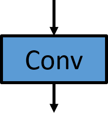
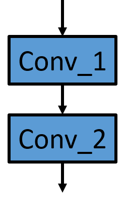
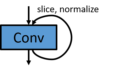
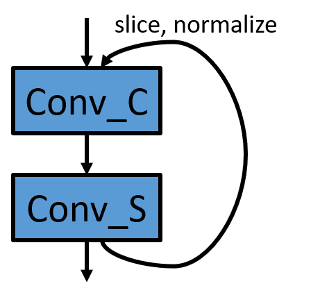
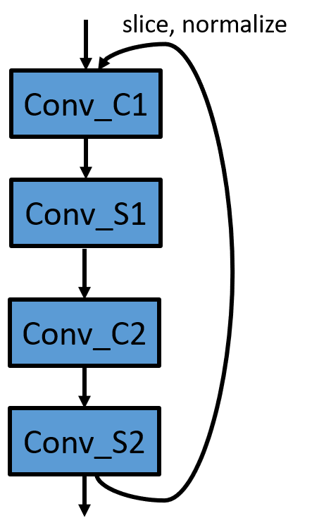
Figure 4: Convolution blocks that we evaluate: (a) Single convolution, (b) Double convolution, (c) Recurrent convolution, (d) Recurrent double convolution, (e) Recursive convolution. $Conv\_C$ stands for cross-channel $1\times 1$ convolution, $Conv\_S$ stands for channel-wise spatial convolution. (f) Recursive quadruple convolution.

4 Experiments

Conv Block	Initial Channels	Scaling	CIFAR-10	Parameters	CIFAR-100	Parameters
type 4	16	3/4	93.49%	214330	68.15%	220180
type 4	32	3/4	95.47%	849130	76.05%	860740
type 4	64	3/4	96.20%	3380170	79.80%	3403300
type 4	128	3/4	96.68%	13488010	81.75%	13534180
type 6	64	3/4	95.24%	421770	78.99%	444900

Table 1: CIFAR accuracies for ECN-6

ECN-6

3x3 Conv

$\begin{bmatrix}CascadedConvBlock\\ FractionalScaling\end{bmatrix}\times 6$

global average pooling

Softmax

Table 2: ECN-6 architecture

4.1 Datasets

We evaluate ECN over three datasets: CIFAR-10, CIFAR-100 [21], and ImageNet-32 [3]. These datasets consist of 32x32 pixel images. CIFAR-10 has 10 classes, CIFAR-100 has 100 classes, and ImageNet-32 has 1000 classes. We employ standard methods of data augmentation, including horizontal image flips, and random 32x32 crops of zero padded images, with 4 pixel padding. CIFAR-10 and CIFAR-100 each contains 50,000 training samples, and 10,000 testing samples. ImageNet-32 contains images of ImageNet [7], downsampled to 32x32 pixels; it contains 1.2 million training samples, and 50 thousand validation samples.

4.2 Results

The ECN network we use has a shape where feature map dimensions consistently decrease in size; it is constructed by iteratively stacking cascading layers until the feature map size is below a preset threshold (4 pixels). In our experiments we fix the number of iterations in Blocks 3, 4, 5, and 6 to $3$.

In table 2 we employed a scaling factor of $\frac{3}{4}$, resulting in an evenly cascaded structure with 6 cascading layers (ECN-6). We report results for differently scaled structures using block 4, and one more result using a more efficient design using block 6. At the beginning of the network, a convolution is used to transform the channel count of the input to $init\_channels$, which takes the value 16, 32, 64, or 128. In each consecutive layer, we generate channels of high level features with a growth rate of $init\_channels\times 2\times(1-scaling\_factor)$, corresponding to 8, 16, 32, 64 respectively in the four networks. The overall network architecture can be found in table 2. Here a cascaded convolution block [27] represents using one convolution block and grouping the results into a low level branch and a high level branch. Global average pooling is used to convert the final feature map into a vector for classification. To avoid overfitting we also insert dropout after ReLU activations for the 3 largest networks in table 2. The dropout rates range from 0.03-0.25. We use stochastic gradient descent to train the network for 2000 epochs with a batch size of 512, for CIFAR10 and CIFAR100, and for 50 epochs and a batch size of 512 for ImageNet-32. The training is scheduled with an initial learning rate of 0.1 and followed by cosine annealing learning rates. The results can be found in table 2.

ImageNet32	Params	Top-1 error	Top-5 error
WRN-28-1 [33]	0.44M	67.97%	42.49%
WRN-28-2 [33]	1.6M	56.92%	30.92%
WRN-28-5 [33]	9.5M	45.36%	21.36%
WRN-28-10 [33]	37.1M	40.96%	18.87%
ECN-6, block 6 (32)	0.24M	63.91%	38.50%
ECN-3, block 6 (64)	0.48M	59.05%	33.68%
ECN-6, block 6 (64)	0.68M	55.51%	30.26%
ECN-6, block 6 (128)	2.1M	46.29%	21.92%
ECN-3, block 4 (128)	7.8M	45.10%	21.06%
ECN-6, block 4 (128)	14.0M	41.87%	18.61%

Table 3: Results on the ImageNet-32 dataset, for WideResNet [33], and ECN (channel count)

Our studies on ImageNet-32 demonstrate ECN’s potential to generalize to larger scale datasets. We evaluate ECN-3 and ECN-6, corresponding to scaling rates of $\frac{1}{2}$ and $\frac{3}{4}$, over ImageNet-32. We use initial channel counts of 32, 64, and 128, and report results in table 3, with channel counts given in parentheses. ECN-6 is more efficient than the strong baseline results reported in WideResNet [33]. An ECN-6 network using only 2 million parameters shows comparable results to a WideResNet architecture using 9.5 million parameters. ECN with block 4 produces competitive results using smaller number of parameters than WideResNet. ECN-3, which has 3 cascading layers and 7 million parameters outperforms the 9.5 million parameter WRN-28-5 result. A larger ECN-6 network using block 4 with 14 million parameters achieves accuracy that is comparable to WRN-28-10, which contains 37.1 million parameters.

Model	Params	CIFAR-10	CIFAR-100
VGG-16 pruned[23]	5.4M	6.60	25.28
VGG-19 pruned[25]	2.3M	6.20	-
VGG-19 pruned[25]	5M	-	26.52
Resnet-56 pruned[23]	.73M	6.94	-
Resnet-110 pruned[23]	1.68M	6.45	-
Resnet 164-B pruned[25]	1.21M	5.27	23.91
DenseNet-40-pruned[25]	.66M	5.19	25.28
CondenseNet-94[15]	.33M	5.00	24.08
CondenseNet-86 [15]	.52M	5.00	23.64
ECN, Block 6	.42M	4.76	21.01

Table 4: Error rate comparison with state-of-the-art efficient architectures

Model	Params	CIFAR-10	CIFAR-100
ResNet-1001[11]	16.1M	4.62	22.71
Stochastic-Depth-1202[17]	19.4M	4.91	-
Wide-ResNet-28[33]	36.5M	4	19.25
ResNeXt-29[32]	68.1M	3.58	19.25
DenseNet-BC-190[16]	25.6M	3.46	17.18
NASNet-A*[15]	3.3M	3.41	-
CondenseNet*light-160[15]	3.1M	3.46	17.55
CondenseNet-182[15]	4.2M	3.76	18.47
ECN, Block4	3.3M	3.8	20.2
ECN, Block4	13.3M	3.32	18.25

Table 5: Error rate comparison with state-of-the-art architectures

4.3 Comparison of Convolution Blocks over CIFAR10 and CIFAR100

We have compared the six block designs over CIFAR10 and CIFAR100 using various sized networks. The networks are trained for 500 epochs. We tested scaling factors $\frac{1}{2},\frac{3}{4},$ and $\frac{7}{8}$, and the corresponding networks have $3,6,$ and $12$ cascading layers. The growth rates are calculated using the same strategy as explained above. For these experiments we use 3-stage learning rate scheduling, decreasing the learning rate at $40\%$ and $80\%$ total epoch count by a factor of 10. We set batch size to 512 for CIFAR-10. For CIFAR-100 a batch size of 128 usually leads to better performance, and we report the better of size 128 and size 512 batches. The results over CIFAR-10 and CIFAR-100 can be found in tables 6 and 7, respectively.

By comparing Blocks 1 and Blocks 3 in tables 6 and 7, and Fig. 5, we found that reusing the convolution weights via recurrent connections significantly improves performance, while maintaining a small network size. When the convolution block becomes powerful, and especially when the model gets large, the improvement due to recurrent connections becomes smaller (Blocks 2 vs Blocks 4). Still, we find a surprise here that through recurrent connections even the single convolution can perform competitively with the widely used double convolution, using the same number of parameters (Fig. 5). The optimal balance between depth and width varies from block to block. Our most efficient convolution block is block 6, which uses recursive quadruple convolutions. We reach state-of-the-art efficiency and the best results are reported in the last row of table 2. It is noteworthy that although using separable convolution [14] reduces the number of parameters, the gain in efficiency also comes with a decrease in accuracy. The effective reduction in parameters enabled by using separable convolutions in ECN blocks $5$ and $6$ is around 2 fold to 4 fold.

When compared to other state-of-the-art efficient architecture designs, listed in table 5, ECN using block 6 achieves the lowest error rate without using any pruning methods. This is significant, as a simple and principled architecture design is proving to be better than sophisticated methods such as pruning described in [25], [23] and even better than [15] with smaller parameter count (Figs. 6,  7). On the other hand, ECN block 4 does relatively well compared to other architectures listed in table 5 that are using more advanced designs than ours.

We have shown that there are avenues for improving the performance of convolutional networks by using principled designs like ECN. Even the simplest designs can reach state-of-the-art performance. Due to limitations in space and computational resources, only the 6 basic block designs are evaluated. More advanced block designs can modularly replace our basic block designs and potentially produce even better numbers.

CIFAR-10		Block 1		Block 2		Block 3		Block 4		Block 5		Block 6
Ch	Sc	Acc	Params	Acc	Params	Acc	Params	Acc	Params	Acc	Params	Acc	Params
16	1/2	83.35%	47482	89.71%	114586	88.59%	47866	91.84%	115546	84.56%	9066	88.59%	19514
16	3/4	88.58%	97258	92.04%	212410	90.96%	98122	92.57%	214330	87.90%	17090	89.92%	35370
16	7/8	90.12%	195082	93.26%	407194	91.51%	196906	93.12%	411034	89.35%	32946	91.02%	66986
32	1/2	87.88%	187114	92.40%	454954	91.66%	187882	93.86%	456874	89.78%	28362	91.47%	64106
32	3/4	91.13%	385738	94.09%	845290	93.15%	387466	94.59%	849130	91.04%	55418	93.36%	117450
32	7/8	92.70%	776074	94.36%	1622506	93.93%	779722	94.67%	1630186	92.64%	108762	93.87%	223754
64	1/2	90.41%	742858	94.41%	1813066	94.39%	744394	95.29%	1816906	92.25%	97674	93.59%	228554
64	3/4	93.53%	1536394	95.43%	3372490	95.24%	1539850	95.66%	3380170	93.96%	195818	94.87%	421770
64	7/8	94.65%	3095818	95.75%	6477514	95.63%	3103114	95.68%	6492874	94.54%	389034	94.82%	806666

Table 6: Comparison of convolution blocks on the CIFAR-10 dataset

CIFAR-100		Block 1		Block 2		Block 3		Block 4		Block 5		Block 6
Ch	Sc	Acc	Params	Acc	Params	Acc	Params	Acc	Params	Acc	Params	Acc	Params
16	1/2	53.93%	53332	64.93%	120436	59.64%	53716	66.45%	121396	54.88%	14916	61.95%	25364
16	3/4	61.50%	103108	68.45%	218260	63.62%	103972	67.95%	220180	59.96%	22940	64.86%	41220
16	7/8	65.40%	200932	71.23%	413044	66.43%	202756	71.26%	416884	63.21%	38796	66.71%	72836
32	1/2	62.17%	198724	71.12%	466564	68.19%	199492	72.72%	468484	64.85%	39972	69.44%	75716
32	3/4	68.98%	397348	75.02%	856900	71.66%	399076	75.62%	860740	67.61%	67028	71.34%	129060
32	7/8	71.72%	787684	76.04%	1634116	73.16%	791332	76.42%	1641796	70.36%	120372	73.22%	235364
64	1/2	67.02%	765988	75.47%	1836196	74.00%	767524	77.13%	1840036	70.23%	120804	74.25%	251684
64	3/4	73.79%	1559524	78.64%	3395620	76.67%	1562980	79.03%	3403300	73.70%	218948	76.80%	444900
64	7/8	74.87%	3118948	79.57%	6500644	77.76%	3126244	80.07%	6516004	75.38%	412164	76.93%	829796

Table 7: Comparison of convolution blocks on the CIFAR-100 dataset

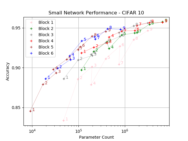
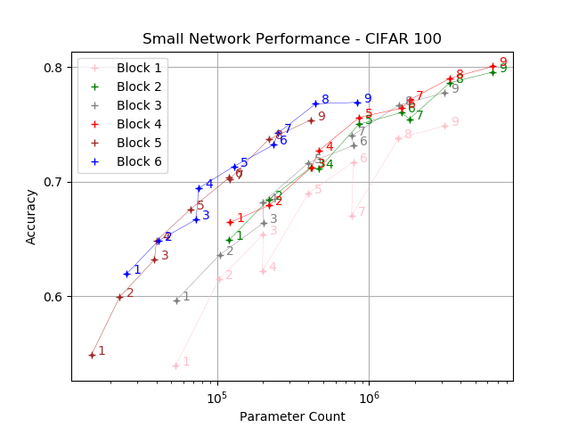
Figure 5: Relationship between network parameter count, block category, and classification accuracy for (a) CIFAR-10 and (b) CIFAR-100 datasets. The results are labeled according to the rows in which they appear in tables 6 and  7.

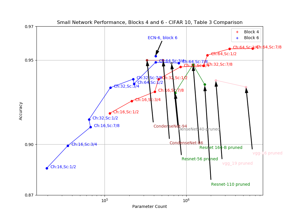
Figure 6: Comparison between parameter count and classification accuracy over CIFAR-10 for ECN with blocks 4 and 6 and architectures listed in table  5. Additionally, our best result using ECN-6 with block 6, attained through longer training, is plotted as “ECN-6, block 6”.

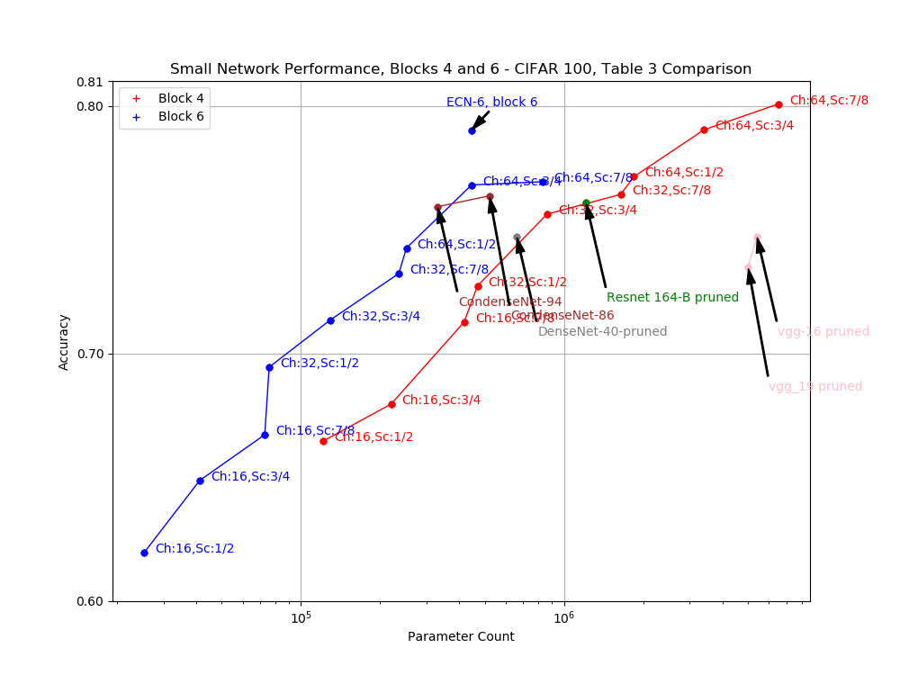
Figure 7: Comparison between parameter count and classification accuracy over CIFAR-100 for ECN with blocks 4 and 6 and architectures listed in table  5. Additionally, our best result using ECN-6 with block 6, attained through longer training, is plotted as “ECN-6, block 6”.

5 Acknowledgement

The support of ONR under grant award N00014-17-1-2622 and the support of the National Science Foundation under grants SMA 1540916 and CNS 1544787 are greatly acknowledged.

6 Conclusion

Taking inspiration from cascading methods in wavelet packet decomposition, we have developed Evenly Cascaded convolutional Networks (ECN) for image tasks. ECN differs from other networks in the use two interacting streams - a high-level feature stream and a low-level feature stream. ECN’s two streams allow for the promulgation of low-level features throughout the entire network, as well as the modulation of those low-level features using advanced perspectives from high-level features. The explicit use of multilevel features not only leads to highly capable networks but provides shortcuts for the training process. Additionally, ECN is structured such that feature map dimensions decrease in a consistent manner, removing burdens of ad hoc architecture design, and potentially improving feature preservation and utility. We have evaluated ECN over CIFAR-10 and CIFAR-100, obtaining state-of-the-art performance, for both datasets, for small network settings; and over ImageNet-32 ECN obtains competitive results.

References

- [1] Yoshua Bengio, Pascal Lamblin, Dan Popovici, and Hugo Larochelle. Greedy layer-wise training of deep networks. In B. Schölkopf, J. C. Platt, and T. Hoffman, editors, Advances in Neural Information Processing Systems 19, pages 153–160. MIT Press, 2007.
- [2] Yunpeng Chen, Jianan Li, Huaxin Xiao, Xiaojie Jin, Shuicheng Yan, and Jiashi Feng. Dual path networks. In I. Guyon, U. V. Luxburg, S. Bengio, H. Wallach, R. Fergus, S. Vishwanathan, and R. Garnett, editors, Advances in Neural Information Processing Systems 30, pages 4467–4475. Curran Associates, Inc., 2017.
- [3] Patryk Chrabaszcz, Ilya Loshchilov, and Frank Hutter. A downsampled variant of imagenet as an alternative to the CIFAR datasets. CoRR, abs/1707.08819, 2017.
- [4] R. R. Coifman and M. V. Wickerhauser. Entropy-based algorithms for best basis selection. IEEE Trans. Inf. Theor., 38(2):713–718, September 2006.
- [5] Matthieu Courbariaux and Yoshua Bengio. Binarynet: Training deep neural networks with weights and activations constrained to +1 or -1. CoRR, abs/1602.02830, 2016.
- [6] J. Dai, H. Qi, Y. Xiong, Y. Li, G. Zhang, H. Hu, and Y. Wei. Deformable Convolutional Networks. ArXiv e-prints, March 2017.
- [7] J. Deng, W. Dong, R. Socher, L. J. Li, Kai Li, and Li Fei-Fei. Imagenet: A large-scale hierarchical image database. In 2009 IEEE Conference on Computer Vision and Pattern Recognition, pages 248–255, June 2009.
- [8] Benjamin Graham. Fractional max-pooling. arXiv preprint arXiv:1412.6071, 2014.
- [9] Song Han, Huizi Mao, and William J. Dally. Deep compression: Compressing deep neural network with pruning, trained quantization and huffman coding. CoRR, abs/1510.00149, 2015.
- [10] Kaiming He, Xiangyu Zhang, Shaoqing Ren, and Jian Sun. Deep residual learning for image recognition. In Proceedings of the IEEE Conference on Computer Vision and Pattern Recognition, pages 770–778, 2016.
- [11] Kaiming He, Xiangyu Zhang, Shaoqing Ren, and Jian Sun. Identity mappings in deep residual networks. CoRR, abs/1603.05027, 2016.
- [12] Geoffrey E. Hinton, Oriol Vinyals, and Jeffrey Dean. Distilling the knowledge in a neural network. CoRR, abs/1503.02531, 2015.
- [13] Sepp Hochreiter and Jürgen Schmidhuber. Long short-term memory. Neural computation, 9(8):1735–1780, 1997.
- [14] Andrew G. Howard, Menglong Zhu, Bo Chen, Dmitry Kalenichenko, Weijun Wang, Tobias Weyand, Marco Andreetto, and Hartwig Adam. Mobilenets: Efficient convolutional neural networks for mobile vision applications. CoRR, abs/1704.04861, 2017.
- [15] Gao Huang, Shichen Liu, Laurens van der Maaten, and Kilian Q. Weinberger. Condensenet: An efficient densenet using learned group convolutions. CoRR, abs/1711.09224, 2017.
- [16] Gao Huang, Zhuang Liu, and Kilian Q. Weinberger. Densely connected convolutional networks. arXiv preprint arXiv:1608.06993, 2016.
- [17] Gao Huang, Yu Sun, Zhuang Liu, Daniel Sedra, and Kilian Q. Weinberger. Deep networks with stochastic depth. CoRR, abs/1603.09382, 2016.
- [18] Forrest N. Iandola, Matthew W. Moskewicz, Khalid Ashraf, Song Han, William J. Dally, and Kurt Keutzer. Squeezenet: Alexnet-level accuracy with 50x fewer parameters and <1mb model size. CoRR, abs/1602.07360, 2016.
- [19] Sergey Ioffe and Christian Szegedy. Batch normalization: Accelerating deep network training by reducing internal covariate shift. CoRR, abs/1502.03167, 2015.
- [20] Max Jaderberg, Karen Simonyan, Andrew Zisserman, and Koray Kavukcuoglu. Spatial transformer networks. CoRR, abs/1506.02025, 2015.
- [21] Alex Krizhevsky and Geoffrey Hinton. Learning multiple layers of features from tiny images, 2009.
- [22] Alex Krizhevsky, Ilya Sutskever, and Geoffrey E Hinton. Imagenet classification with deep convolutional neural networks. In Advances in neural information processing systems, pages 1097–1105, 2012.
- [23] Hao Li, Asim Kadav, Igor Durdanovic, Hanan Samet, and Hans Peter Graf. Pruning filters for efficient convnets. CoRR, abs/1608.08710, 2016.
- [24] Ming Liang and Xiaolin Hu. Recurrent convolutional neural network for object recognition. In The IEEE Conference on Computer Vision and Pattern Recognition (CVPR), June 2015.
- [25] Zhuang Liu, Jianguo Li, Zhiqiang Shen, Gao Huang, Shoumeng Yan, and Changshui Zhang. Learning efficient convolutional networks through network slimming. CoRR, abs/1708.06519, 2017.
- [26] S. Mallat. Understanding deep convolutional networks. Philosophical Transactions of the Royal Society of London Series A, 374:20150203, April 2016.
- [27] Stphane Mallat. A Wavelet Tour of Signal Processing, Third Edition: The Sparse Way. Academic Press, Inc., Orlando, FL, USA, 3rd edition, 2008.
- [28] D. E. Rumelhart, G. E. Hinton, and R. J. Williams. Parallel distributed processing: Explorations in the microstructure of cognition, vol. 1. chapter Learning Internal Representations by Error Propagation, pages 318–362. MIT Press, Cambridge, MA, USA, 1986.
- [29] Karen Simonyan and Andrew Zisserman. Very deep convolutional networks for large-scale image recognition. CoRR, abs/1409.1556, 2014.
- [30] Richard Socher, Brody Huval, Bharath Bath, Christopher D Manning, and Andrew Y Ng. Convolutional-recursive deep learning for 3d object classification. In Advances in neural information processing systems, pages 656–664, 2012.
- [31] Rupesh Kumar Srivastava, Klaus Greff, and Jürgen Schmidhuber. Highway networks. CoRR, abs/1505.00387, 2015.
- [32] Saining Xie, Ross B. Girshick, Piotr Dollár, Zhuowen Tu, and Kaiming He. Aggregated residual transformations for deep neural networks. CoRR, abs/1611.05431, 2016.
- [33] Sergey Zagoruyko and Nikos Komodakis. Wide residual networks. CoRR, abs/1605.07146, 2016.
- [34] Matthew D. Zeiler and Rob Fergus. Visualizing and understanding convolutional networks. CoRR, abs/1311.2901, 2013.
- [35] Ting Zhang, Guo-Jun Qi, Bin Xiao, and Jingdong Wang. Interleaved group convolutions for deep neural networks. CoRR, abs/1707.02725, 2017.
- [36] Xiangyu Zhang, Xinyu Zhou, Mengxiao Lin, and Jian Sun. Shufflenet: An extremely efficient convolutional neural network for mobile devices. CoRR, abs/1707.01083, 2017.