Quantum critical phenomena of excitonic insulating transition in two dimensions

Abstract

We study the quantum criticality of the phase transition between Dirac semimetal and excitonic insulator in two dimensions. Even though the system has a semimetallic ground state, there are observable effects of excitonic pairing at finite temperatures and/or finite energies, provided that the system is in proximity to excitonic insulating transition. To determine the quantum critical behavior, we consider three potentially important interactions, including the Yukawa coupling between Dirac fermions and excitonic order parameter fluctuation, the long-range Coulomb interaction, and the disorder scattering. We employ the renormalization group technique to study how these interactions affect quantum criticality and also how they influence each other. We first investigate the Yukawa coupling in the clean limit, and show that it gives rise to typical non-Fermi liquid behavior. Adding random scalar potential to the system always turns such a non-Fermi liquid into a compressible diffusive metal. In comparison, the non-Fermi liquid behavior is further enhanced by random vector potential, but is nearly unaffected by random mass. Incorporating the Coulomb interaction may change the results qualitatively. In particular, the non-Fermi liquid state is protected by the Coulomb interaction for weak random scalar potential, and it becomes a diffusive metal only when random scalar potential becomes sufficiently strong. When random vector potential or random mass coexists with Yukawa coupling and Coulomb interaction, the system is stable non-Fermi liquid state, with fermion velocities flowing to constants in the former case and being singularly renormalized in the latter case. These quantum critical phenomena can be probed by measuring observable quantities. We also find that, while the fermion velocity anisotropy is not altered by the excitonic quantum fluctuation, it may be driven by the Coulomb interaction to flow to the isotropic limit.

I Introduction

In the past decade, the unconventional properties of various Dirac/Weyl semimetal (SM) materials Sarma11 ; Kotov12 ; Vafek14 ; Wehling14 ; Wan11 ; Weng16 ; FangChen16 ; Yan17 ; Hasan17 ; Armitage18 have been investigated extensively. Many of the unconventional properties are related to the existence of isolated Dirac/Weyl points, at which the conduction and valence bands touch. When the chemical potential is tuned to exactly the Dirac points, the fermion density of states (DOS) vanishes at the Fermi level. As a result, the Coulomb interaction is long-ranged due to the absence of static screening. Extensive previous studies Kotov12 ; Gonzalez99 ; Hofmann14 ; Sharma16 ; Goswami11 ; Hosur12 ; Hofmann15 ; Throckmorton15 ; Sharma18 ; Yang14 ; Abrikosov72 ; Abrikosov71 ; Abrikosov74 ; Moon13 ; Herbut14 ; Janssen15 ; Dumitrescu15 ; Janssen17 ; Huh16 ; Cho16 ; Isobe16B ; Lai15 ; Jian15 ; Zhang17 ; WangLiuZhang17MWSM have revealed that the Coulomb interaction leads to a variety of unconventional low-energy behaviors.

Among all the known SM materials, two-dimensional Dirac SM, abbreviated as 2D DSM hereafter, has been studied most extensively, usually in the context of graphene. Renormalization group (RG) analysis Shankar94 ; Kotov12 has revealed that the long-range Coulomb interaction is marginally irrelevant in the weak-coupling regime. When the Coulomb interaction is strong enough, the originally massless fermions can acquire a dynamical mass gap via the formation of stable particle-hole pairs CastroNetoPhysics09 ; Khveshchenko01 ; Gorbar02 ; Khveshchenko04 ; Liu09 ; Khveshchenko09 ; Gamayun10 ; Sabio10 ; Zhang11 ; Liu11 ; WangLiu11A ; WangLiu11B ; WangLiu12 ; Popovici13 ; WangLiu14 ; Gonzalez15 ; Carrington16 ; Sharma17 ; Xiao17 ; Carrington18 ; Gamayun09 ; WangJianhui11 ; Katanin16 ; Gonzalez10 ; Gonzalez12 ; Drut09A ; Drut09B ; Drut09C ; Armour10 ; Armour11 ; Buividovich12 ; Ulybyshev13 ; Smith14 ; Juan12 ; Kotikov16 ; Gonzalez14 ; Braguta16 ; Xiao18 ; Janssen16 ; WangLiuZhangSemiDSM . This gap generating scenario is non-perturbative, and has the same picture as excitonic pairing, a notion proposed decades ago Keldysh64 ; Jerome67 . In the special case of 2D DSM, such an excitonic gap dynamically breaks a continuous chiral (sublattice) symmetry, which can be regarded as a condensed-matter realization of the dynamical chiral symmetry breaking Nambu61 ; Miransky94 . The finite gap opened at the Dirac point drives the SM to undergo a quantum phase transition (QPT) into an excitonic insulator (EI). The EI is induced only when the effective interaction strength, denoted by $\alpha$, exceeds some critical value $\alpha_{c}$, which defines SM-EI quantum critical point (QCP).

In recent years, the possibility of SM-EI transition in graphene has been investigated by means of various analytical and numerical techniques. Early calculations CastroNetoPhysics09 ; Khveshchenko01 ; Gorbar02 ; Khveshchenko04 ; Liu09 ; Khveshchenko09 ; Gamayun10 ; Drut09A ; Drut09B ; Drut09C predicted that the Coulomb interaction in suspended graphene is strong enough to open an excitonic gap at zero temperature. Specifically, the critical value $\alpha_{c}$ was claimed to be smaller than the physical value $\alpha=2.16$. However, no visible experimental evidence for excitonic gap has been observed at low temperatures Elias11 ; Mayorov12 . More careful numerical calculations WangLiu12 ; Gonzalez15 ; Carrington16 ; Ulybyshev13 ; Smith14 ; Kotikov16 revealed that the critical value $\alpha_{c}$ is actually larger than $2.16$, which implies that the Coulomb interaction cannot generate a finite excitonic gap. Owing to the conceptual importance and also the potential technical applications, theorists are still searching for possible approaches to promote excitonic pairing in various SM materials. For instance, it was proposed that excitonic pairing may be promoted by an additional short-range repulsive interaction Liu09 ; Gamayun10 ; WangLiu12 or by certain extrinsic effects, such as strain Tang15 .

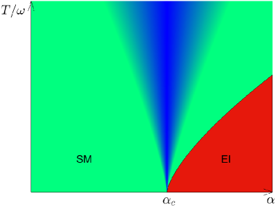
Figure 1: Global phase diagram of 2D DSM on the $\alpha$-$T$ or $\alpha$-$\omega$ plane. Here, $\omega$ stands for the fermion energy. Deep in the insulating phase, the fermions are suppressed at low energies. Deep in the semimetallic phase, the Coulomb interaction is too weak to form excitonic pairs. The excitonic insulating transition occurs as $\alpha$ increases up to $\alpha_{c}$ at $T=0$. This point is broadened into a finite quantum critical regime at finite $T$ and/or finite $\omega$. The excitonic quantum fluctuation has observable effects in the whole quantum critical regime.

Most previous works on SM-EI QPT have focused on the precise calculation of $\alpha_{c}$ at zero temperature ($T=0$) by means of various techniques CastroNetoPhysics09 ; Khveshchenko01 ; Gorbar02 ; Khveshchenko04 ; Liu09 ; Khveshchenko09 ; Gamayun10 ; Sabio10 ; Zhang11 ; Liu11 ; WangLiu11A ; WangLiu11B ; WangLiu12 ; Popovici13 ; WangLiu14 ; Gonzalez15 ; Carrington16 ; Sharma17 ; Xiao17 ; Carrington18 ; Gamayun09 ; WangJianhui11 ; Katanin16 ; Gonzalez10 ; Gonzalez12 ; Drut09A ; Drut09B ; Drut09C ; Armour10 ; Armour11 ; Buividovich12 ; Ulybyshev13 ; Smith14 ; Juan12 ; Kotikov16 ; Gonzalez14 ; Braguta16 ; Xiao18 ; Janssen16 ; WangLiuZhangSemiDSM . In this paper, we propose to explore the signatures of excitonic pairing at finite $T$ and/or finite energy $\omega$. Here is our logic: even though the exact zero-$T$ ground state of suspended graphene (or other 2D DSMs) is gapless, the quantum fluctuation of excitonic pairs still have observable effects at finite $T$ and/or $\omega$ if the system is in the quantum critical regime around the putative SM-EI QCP. Recent Monte Carlo simulations Ulybyshev13 and Dyson-Schwinger equation study Carrington18 both suggest that the value $\alpha_{c}$ is not far from the physical value of suspended graphene. As illustrated in the schematic phase diagram Fig. 1, if $\alpha$ is slightly smaller than $\alpha_{c}$, no excitonic gap is opened at $T=0$ and the excitonic order parameter has a vanishing mean-value. However, the quantum fluctuation of excitonic order parameter is not negligible at finite $T$ and/or $\omega$ and may lead to considerable corrections to observable quantities. For instance, the nuclear-magnetic-resonance measurements performed by Hirata et al. Hirata17 indicate that the compound $\alpha$-(BEDT-TTF)₂I₃ is close to an SM-EI QCP and that the excitonic fluctuation results in singular corrections to the nuclear magnetic resonance relaxation rate.

We study the quantum critical phenomena emerging in the broad quantum critical regime around SM-EI QCP, with the aim to explore observable effects of excitonic pairing. For this purpose, we take suspended graphene (typical 2D DSM) as our starting model, and calculate the interaction corrections to some observable quantities of Dirac fermions. In this regime, the gapless fermions interact with the quantum critical fluctuation of excitonic order parameter, which is described by a Yukawa coupling term. The long-range Coulomb interaction is still present and needs to be properly taken into account. Moreover, there is always certain amount of quenched disorder Kotov12 in realistic materials, and the fermion-disorder coupling might play a vital role. The actual quantum critical phenomena cannot be accurately determined if one or more of these interactions are naively ignored or improperly treated. We emphasize that, these three kinds of interaction may have very complicated mutual influence. To make a generic analysis, we will treat all the three kinds of interaction on equal footing and study their interplay carefully.

As the first step, we treat the Yukawa coupling in the clean limit, and demonstrate that this coupling leads to strong violation of Fermi liquid (FL) theory. Indeed, the quasiparticle residue $Z_{f}$ vanishes at low energies, and the fermion DOS $\rho(\omega)$ receives power-law corrections from the excitonic fluctuation. Both of these two features are typical non-Fermi-liquid (NFL) behaviors. If the fermion dispersion is originally anisotropic, the ratio between two fermion velocities is unrenormalized.

The next step is to incorporate quenched disorder and analyze its interplay with the Yukawa coupling. We find that the resultant low-energy properties depend sensitively on the nature of the disorder. Adding random scalar potential (RSP) to the system always turns the NFL caused by Yukawa coupling in the clean limit into a compressible diffusive metal (CDM). The CDM state is characterized by the generation of a finite zero-energy fermion DOS and a constant zero-$T$ disorder scattering rate. Different from RSP, random vector potential (RVP) tends to further enhance the NFL behavior, whereas random mass (RM) has negligible effects on the system.

We finally incorporate the Coulomb interaction, and find that it changes the above results qualitatively. In the case of weak RSP, the Coulomb interaction suppresses disorder scattering and as such renders the stability of the NFL state caused by Yukawa coupling. However, such a NFL is converted into CDM once RSP becomes sufficiently strong. The combination of Yukawa coupling, Coulomb interaction, and RVP produces a stable NFL state in which the two fermion velocities flow to constant values in the zero energy limit. When the Yukawa coupling, Coulomb interaction, and RM are considered simultaneously, we show that the Coulomb interaction is marginally irrelevant and RM is irrelevant. These results indicate that the true quantum critical phenomena are determined by a delicate interplay of excitonic fluctuation, Coulomb interaction, and disorder scattering.

Our results might be applied to understand some 2D DSM materials, such as uniaxially strained graphene Sharma17 ; Xiao17 and organic compound $\alpha$-(BEDT-TTF)₂I₃ Hirata17 . In these systems, the fermion velocities along different directions may be unequal. It is thus necessary to examine how interactions change the anisotropy. According to our RG analysis, the fermion velocity anisotropy is unaffected by the excitonic fluctuation, but could be significantly suppressed by the Coulomb interaction.

The rest of the paper will be arranged as following. The model is presented in Sec. II. The RG equations for the corresponding parameters are shown in Sec. III. The numerical results for different conditions are given and analyzed in Sec. IV. The mains results are summarized in Sec. V. The detailed derivation of the RG equations can be found in Appendices.

II The model

The fermion energy dispersion in intrinsic graphene is isotropic. It becomes anisotropic when graphene is deformed. Generically, the action of free 2D Dirac fermions with anisotropic dispersion is given by

$$S_{f}=\sum_{\sigma=1}^{N}\int_{\tau,\mathbf{x}}\bar{\Psi}_{\sigma}(\tau,\mathbf{x})\left[\partial_{\tau}\gamma_{0}+\mathcal{H}_{f}\right]\Psi_{\sigma}(\tau,\mathbf{x}),$$ (1)

where $\int_{\tau,\mathbf{x}}\equiv\int d\tau\int d^{2}\mathbf{x}$ and $\mathcal{H}_{f}=-iv_{1}\nabla_{1}\gamma_{1}-iv_{2}\nabla_{2}\gamma_{2}$. Here, $\Psi$ is a four-component spinor, and $\bar{\Psi}=\Psi^{{\dagger}}\gamma_{0}$. The matrices $\gamma_{0,1,2}$ are defined as $\gamma_{0,1,2}=\left(\tau_{3},-i\tau_{2},i\tau_{1}\right)\otimes\tau_{3}$ in terms of Pauli matrices $\tau_{i}$ with $i=1,2,3$. The gamma matrices satisfy the anti-commutative rule $\left\{\gamma_{\mu},\gamma_{\nu}\right\}=2\mathrm{diag}(1,-1,-1)$. The fermion species is denoted by $\sigma$, which sums from $1$ to $N$. Fermion flavor $N$ is assumed to be a general large integer. We use $v_{1}$ and $v_{2}$ to represent the fermion velocities along two orthogonal directions.

The action of the quantum fluctuation of excitonic order parameter can be written as

$$S_{b}=\int_{\tau,\mathbf{x}}\left[\frac{1}{2}\left(\partial_{\tau}\phi\right)^{2}+\frac{c^{2}}{2}\left(\mathbf{\nabla}\phi\right)^{2}+\frac{r}{2}\phi^{2}+\frac{u}{24}\phi^{4}\right],$$ (2)

where $c$ is the boson velocity. Varying boson mass $r$ tunes the QPT between SM and EI phases. At the QCP, the mass vanishes, i.e., $r=0$, and the boson field $\phi$ describes the quantum critical fluctuation of excitonic order parameter. The quartic self-interacting term has a coupling constant $u$. The Yukakwa coupling between fermions and excitonic order parameter is given by

$$S_{fb}=\lambda\sum_{\sigma=1}^{N}\int_{\tau,\mathbf{x}}\phi\bar{\Psi}_{\sigma}\Psi_{\sigma},$$ (3)

where $\lambda$ is the corresponding coupling constant.

The excitonic pairing originates from the Coulomb interaction between fermions and their anti-fermions (holes). Inside the EI phase, a finite gap is opened at the Fermi level and strongly suppresses the low-energy fermion DOS. In this case, the Coulomb interaction and even the fermionic degrees of freedom can be neglected, and the low-energy properties of the EI phase is mainly governed by the dynamics of neutral excitons. In contrast, the fermions remain gapless at the SM-EI QCP. The Coulomb interaction between gapless fermions may play an important role at low energies. The action for Coulomb interaction is described by

$$S_{ee}=\frac{1}{4\pi}\sum_{\sigma,\sigma^{\prime}=1}^{N}\int_{\tau,\mathbf{x},\mathbf{x}^{\prime}}\rho_{\sigma}(\tau,\mathbf{x})\frac{e^{2}/\epsilon}{|\mathbf{x}-\mathbf{x}^{\prime}|}\rho_{\sigma}(\tau,\mathbf{x}^{\prime}),$$ (4)

where $\int_{\tau,\mathbf{x},\mathbf{x}^{\prime}}\equiv\int d\tau\int d^{2}\mathbf{x}\int d^{2}\mathbf{x}^{\prime}$. The fermion density operator is defined as $\rho_{\sigma}(\tau,\mathbf{x})=\bar{\Psi}_{\sigma}(\tau,\mathbf{x})\gamma_{0}\Psi_{\sigma}(\tau,\mathbf{x})$. In addition, $e$ is electric charge and $\epsilon$ dielectric constant.

Disorder exists in almost all realistic materials. Many of the low-energy behaviors of fermions are heavily affected by disorder scattering, especially at low $T$. The fermion-disorder coupling is formally described by

$$S_{\mathrm{dis}}=v_{\Gamma}\int d\tau d^{2}\mathbf{x}\bar{\Psi}_{\sigma}(\mathbf{x})\Gamma\Psi_{\sigma}(\mathbf{x})A(\mathbf{x}).$$ (5)

The random field $A(\mathbf{x})$ is assumed to be a Gaussian white noise, i.e., $\langle A(\mathbf{x})\rangle=0$ and $\langle A(\mathbf{x})A(\mathbf{x}^{\prime})\rangle=\Delta\delta^{2}(\mathbf{x}-\mathbf{x}^{\prime})$. Here, $\Delta$ is the impurity concentration, and $v_{\Gamma}$ measures the strength of a single impurity. The disorders are classified by the expression of $\Gamma$ matrix Ludwig94 ; Nersesyan95 ; Altland02 . For $\Gamma_{0}=\gamma_{0}$, $A(\mathbf{x})$ is a RSP. For $\Gamma_{j}=\mathbbm{1}_{4}$, $A(\mathbf{x})$ serves as a RM. In comparison, RVP has two components $A_{1,2}(\mathbf{x})$, characterized by $\Gamma=(\gamma_{1},\gamma_{2})$ and $v_{\Gamma}=(v_{\Gamma 1},v_{\Gamma 2})$.

The free fermion propagator has the form

$$G_{0}(\omega,\mathbf{k})=\frac{1}{-i\omega\gamma_{0}+v_{1}k_{1}\gamma_{1}+v_{1}k_{2}\gamma_{2}}.$$ (6)

The Yukawa coupling can be treated by the RG method in combination with the $1/N$ expansion. Following the scheme developed by Huh and Sachdev Huh08 , we re-scale $\phi$ and $r$ as follows: $\phi\rightarrow\phi/\lambda$ and $r\rightarrow Nr\lambda^{2}$. Accordingly, the bare propagator of $\phi$ is expressed as

$$D_{0}^{A}(\Omega,\mathbf{q})=\frac{1}{\frac{\Omega^{2}+c^{2}\mathbf{q}^{2}}{\lambda^{2}}+Nr}.$$ (7)

Near the QCP, we take $r=0$ and then get

$$D_{0}^{A}(\Omega,\mathbf{q})=\frac{\lambda^{2}}{\Omega^{2}+c^{2}\mathbf{q}^{2}}.$$ (8)

The free boson propagator is drastically altered by the polarization function, which, to the leading order of $1/N$ expansion, is

$$\Pi^{A}(\Omega,\mathbf{q}) = N\int\frac{d\omega}{2\pi}\frac{d^{2}\mathbf{k}}{(2\pi)^{2}}$$ (9)

$$\times\mathrm{Tr}\left[G_{0}(\omega,\mathbf{k})G_{0}(\omega+\Omega,\mathbf{k}+\mathbf{q})\right]$$

$$= \frac{N}{4v_{1}v_{2}}\sqrt{\Omega^{2}+v_{1}^{2}q_{1}^{2}+v_{2}^{2}q_{2}^{2}}.$$

Now the dressed boson propagator becomes

$$D^{A}(\Omega,\mathbf{q})=\frac{1}{\frac{\Omega^{2}+c^{2}\mathbf{q}^{2}}{\lambda^{2}}+\Pi^{A}(\Omega,\mathbf{q})}.$$ (10)

It is obvious that $\Pi^{A}$ dominates over the free term in the low-energy regime. Thus, the above expression can be further simplified to

$$D^{A}(\Omega,\mathbf{q})\approx\frac{1}{\Pi^{A}(\Omega,\mathbf{q})}.$$ (11)

The bare Coulomb interaction is described by

$$D_{0}^{B}(\mathbf{q})=\frac{2\pi e^{2}}{\epsilon|\mathbf{q}|}.$$ (12)

The dynamical screening is encoded in the polarization $\Pi^{B}(\Omega,\mathbf{q})$, whose leading order expression is given by

$$\Pi^{B}(\Omega,\mathbf{q}) = -N\int\frac{d\omega}{2\pi}\frac{d^{2}\mathbf{k}}{(2\pi)^{2}}\mathrm{Tr}\left[\gamma_{0}G_{0}(\omega,\mathbf{k})\gamma_{0}\right.$$ (13)

$$\left.\times G_{0}(\omega+\Omega,\mathbf{k}+\mathbf{q})\right]$$

$$= \frac{N}{8v_{1}v_{2}}\frac{v_{1}^{2}q_{1}^{2}+v_{2}^{2}q_{2}^{2}}{\sqrt{\Omega^{2}+v_{1}^{2}q_{1}^{2}+v_{2}^{2}q_{2}^{2}}}.$$

The dressed Coulomb interaction can be written as

$$D^{B}(\Omega,\mathbf{q})=\frac{1}{\frac{\epsilon|\mathbf{q}|}{2\pi e^{2}}+\Pi^{B}(\Omega,\mathbf{q})}.$$ (14)

In previous works on the quantum criticality of SM-EI transition, the interplay of Yukawa coupling, Coulomb interaction, and disorder has never been systematically studied. Here, we emphasize that all the three interactions could be very important at low energies and thus should be treated equally.

III Renormalization group equations

The interplay of distinct interactions can be handled by means of perturbative RG approach. The detailed RG calculations are presented in the Appendices. In this section, we only list the coupled RG equations of a number of model parameters and then analyze their low-energy properties. The effective model contains several independent parameters, such as $v_{1}$, $v_{2}$, and $v_{\Gamma}$. These parameters are renormalized by interactions. To specify how the interactions alter the fermion dispersion anisotropy, we need to determine the flow of the ratio $v_{2}/v_{1}$. Moreover, to judge whether FL theory is applicable, we should compute the flow equation of the residue $Z_{f}$.

After incorporating three types of interaction in a self-consistent way, we find that the coupled RG equations for $Z_{f}$, $v_{1}$, $v_{2}$, and $v_{2}/v_{1}$ are given by

$$\frac{dZ_{f}}{d\ell} = \left(C_{0}^{A}+C_{0}^{B}-C_{g}\right)Z_{f},$$ (15)

$$\frac{dv_{1}}{d\ell} = \left(C_{0}^{A}+C_{0}^{B}-C_{1}^{A}-C_{1}^{B}-C_{g}\right)v_{1},$$ (16)

$$\frac{dv_{2}}{d\ell} = \left(C_{0}^{A}+C_{0}^{B}-C_{2}^{A}-C_{2}^{B}-C_{g}\right)v_{2},$$ (17)

$$\frac{d\left(v_{2}/v_{1}\right)}{d\ell} = \left(C_{1}^{A}-C_{2}^{A}+C_{1}^{B}-C_{2}^{B}\right)\frac{v_{2}}{v_{1}}.$$ (18)

RG analysis is performed by integrating out the modes defined within the momentum shell $e^{-\ell}\Lambda<|\mathbf{k}|<\Lambda$, where $\Lambda$ is an UV cutoff and $\ell$ is a running parameter Shankar94 . The lowest energy limit is reached as $\ell\rightarrow\infty$. For RSP, the flow equation of $v_{\Gamma}$ takes the form

$$\frac{dv_{\Gamma}}{d\ell}=0.$$ (19)

For the two components of RVP, the flow equations for $v_{\Gamma 1}$ and $v_{\Gamma 2}$ are

$$\frac{dv_{\Gamma 1}}{d\ell}=\left(C_{0}^{A}+C_{0}^{B}-C_{1}^{A}-C_{1}^{B}-C_{g}\right)v_{\Gamma 1},$$ (20)

$$\frac{dv_{\Gamma 2}}{d\ell}=\left(C_{0}^{A}+C_{0}^{B}-C_{2}^{A}-C_{2}^{B}-C_{g}\right)v_{\Gamma 2}.$$ (21)

For RM, the flow equation of $v_{\Gamma}$ is

$$\frac{dv_{\Gamma}}{d\ell} = \left(2C_{0}^{A}+C_{1}^{A}+C_{2}^{A}+2C_{0}^{B}-C_{1}^{B}-C_{2}^{B}\right.$$ (22)

$$\left.-2C_{g}\right)v_{\Gamma}.$$

Here, we introduce a new parameter $C_{g}$ to characterize the effective strength of disorder. For RSP and RM, it is

$$C_{g}=\frac{v_{\Gamma}^{2}\Delta}{2\pi v_{1}v_{2}}.$$ (23)

For RVP, we have

$$C_{g}=\frac{\left(v_{\Gamma 1}^{2}+v_{\Gamma 2}^{2}\right)\Delta}{2\pi v_{1}v_{2}}.$$ (24)

The three coefficients $C_{0}^{A}$, $C_{1}^{A}$, and $C_{2}^{A}$ appearing in the coupled RG equations are

$$C_{0}^{A} = \frac{1}{8\pi^{3}}\int_{-\infty}^{+\infty}dx\int_{0}^{2\pi}d\theta$$ (25)

$$\times\frac{x^{2}-\cos^{2}\theta-(v_{2}/v_{1})^{2}\sin^{2}\theta}{\left(x^{2}+\cos^{2}\theta+(v_{2}/v_{1})^{2}\sin^{2}\theta\right)^{2}}\mathcal{G}^{A}(x,\theta),$$

$$C_{1}^{A} = \frac{1}{8\pi^{3}}\int_{-\infty}^{+\infty}dx\int_{0}^{2\pi}d\theta$$ (26)

$$\times\frac{-x^{2}+\cos^{2}\theta-(v_{2}/v_{1})^{2}\sin^{2}\theta}{\left(x^{2}+\cos^{2}\theta+(v_{2}/v_{1})^{2}\sin^{2}\theta\right)^{2}}\mathcal{G}^{A}(x,\theta),$$

$$C_{2}^{A} = \frac{1}{8\pi^{3}}\int_{-\infty}^{+\infty}dx\int_{0}^{2\pi}d\theta$$ (27)

$$\times\frac{-x^{2}-\cos^{2}\theta+(v_{2}/v_{1})^{2}\sin^{2}\theta}{\left(x^{2}+\cos^{2}\theta+(v_{2}/v_{1})^{2}\sin^{2}\theta\right)^{2}}\mathcal{G}^{A}(x,\theta),$$

where

$$\mathcal{G}^{A}(x,\theta)=\frac{1}{\frac{N}{4v_{2}/v_{1}}\sqrt{x^{2}+\cos^{2}\theta+\left(v_{2}/v_{1}\right)^{2}\sin^{2}\theta}}.$$ (28)

The coefficients $C_{0}^{B}$, $C_{1}^{B}$, and $C_{2}^{B}$ are

$$C_{0}^{B} = \frac{1}{8\pi^{3}}\int_{-\infty}^{+\infty}dx\int_{0}^{2\pi}d\theta$$ (29)

$$\times\frac{-x^{2}+\cos^{2}\theta+(v_{2}/v_{1})^{2}\sin^{2}\theta}{\left(x^{2}+\cos^{2}\theta+(v_{2}/v_{1})^{2}\sin^{2}\theta\right)^{2}}\mathcal{G}^{B}(x,\theta),$$

$$C_{1}^{B} = \frac{1}{8\pi^{3}}\int_{-\infty}^{+\infty}dx\int_{0}^{2\pi}d\theta$$ (30)

$$\times\frac{-x^{2}+\cos^{2}\theta-(v_{2}/v_{1})^{2}\sin^{2}\theta}{\left(x^{2}+\cos^{2}\theta+(v_{2}/v_{1})^{2}\sin^{2}\theta\right)^{2}}\mathcal{G}^{B}(x,\theta),$$

$$C_{2}^{B} = \frac{1}{8\pi^{3}}\int_{-\infty}^{+\infty}dx\int_{0}^{2\pi}d\theta$$ (31)

$$\times\frac{-x^{2}-\cos^{2}\theta+(v_{2}/v_{1})^{2}\sin^{2}\theta}{\left(x^{2}+\cos^{2}\theta+(v_{2}/v_{1})^{2}\sin^{2}\theta\right)^{2}}\mathcal{G}^{B}(x,\theta),$$

with

$$\mathcal{G}^{B}(x,\theta)=\frac{1}{\frac{1}{2\pi\alpha_{1}}+\frac{N}{8v_{2}/v_{1}}\frac{\cos^{2}\theta+(v_{2}/v_{1})^{2}\sin^{2}\theta}{\sqrt{x^{2}+\cos^{2}\theta+(v_{2}/v_{1})^{2}\sin^{2}\theta}}}.$$ (32)

An effective parameter

$$\alpha_{1}=\frac{e^{2}}{\epsilon v_{1}}$$ (33)

is defined to represent the Coulomb interaction strength. The electric charge $e$ is not renormalized due to the absence of logarithmic term in the polarization $\Pi^{B}$ Kotov12 , and $\epsilon$ takes a constant value in any given sample. The value of $\alpha_{1}$ is determined by the renormalization of velocity $v_{1}$.

The coupled flow equations can be simplified. According to Eq. (19), we know that

$$v_{\Gamma}=v_{\Gamma 0}$$ (34)

is independent of $\ell$ for RSP. Thus we re-write $C_{g}$ as

$$C_{g}=\frac{v_{\Gamma 0}^{2}\Delta}{2\pi v_{1}v_{2}}.$$ (35)

The flow equation for $C_{g}$ is given by

$$\frac{dC_{g}}{d\ell} = \left(-2C_{0}^{A}-2C_{0}^{B}+C_{1}^{A}+C_{1}^{B}+C_{2}^{A}+C_{2}^{B}\right.$$ (36)

$$\left.+2C_{g}\right)C_{g}.$$

For RVP, from Eqs. (16), (17), (20), and (21), one gets

$$\frac{d(v_{\Gamma 1}/v_{1})}{d\ell}=0,\qquad\frac{d(v_{\Gamma 2}/v_{2})}{d\ell}=0,$$ (37)

which indicate that

$$\frac{v_{\Gamma 1}}{v_{1}}=\frac{v_{\Gamma 10}}{v_{10}},\qquad\frac{v_{\Gamma 2}}{v_{2}}=\frac{v_{\Gamma 20}}{v_{20}}.$$ (38)

Accordingly, $C_{g}$ now can be written as

$$C_{g}=\frac{\Delta}{2\pi}\left(\frac{v_{\Gamma 10}^{2}}{v_{10}^{2}}\frac{v_{1}}{v_{2}}+\frac{v_{\Gamma 20}^{2}}{v_{20}^{2}}\frac{v_{2}}{v_{1}}\right).$$ (39)

The corresponding RG equation is

$$\frac{dC_{g}}{d\ell}=\frac{\left(v_{\Gamma 1}^{2}-v_{\Gamma 2}^{2}\right)\Delta}{2\pi v_{1}v_{2}}\left(-C_{1}^{A}-C_{1}^{B}+C_{2}^{A}+C_{2}^{B}\right).$$ (40)

For RM, through Eqs. (16), (17), and (22), we obtain the following flow equation

$$\frac{dC_{g}}{d\ell} = \left(2C_{0}^{A}+3C_{1}^{A}+3C_{2}^{A}+2C_{0}^{B}-C_{1}^{B}-C_{2}^{B}\right.$$ (41)

$$\left.-2C_{g}\right)C_{g}.$$

IV Quantum critical phenomena

In this section, we will solve the RG equations and then apply the solutions to analyze the quantum critical phenomena. We adopt the following steps: first, examine the low-energy behaviors induced solely by the quantum critical fluctuation of excitonic order parameter; second, introduce quenched disorder into the system and study its interplay with the Yukawa coupling; finally, investigate the impact of Coulomb interaction on the results.

Although the RG calculations are carried out at $T=0$, it is possible to extract the $T$-dependence of observable quantities from RG results. We can regard $k_{B}T$, where $k_{B}$ is Boltzmann constant, as a free parameter that tunes the energy scale: increasing (decreasing) $T$ amounts to increasing (decreasing) the energy $\omega$. The dependence of observable quantities on $\omega$ and/or $T$ can be computed from the solutions of RG equations as follows. One solves the flow equations at $T=0$ and gets the $\ell$-dependence of model parameters, such as fermion velocities, which leads to the $\ell$-dependence of various observable quantities. On the basis of these results, one converts the $\ell$-dependence of an observable quantity into the $\omega$-dependence of the same quantity at $T=0$ by using the transformation $\omega=\omega_{0}e^{-\ell}$, where $\omega_{0}$ is some high energy, or into the $T$-dependence of the same quantity by using the transformation $T=T_{0}e^{-\ell}$, where $T_{0}$ takes a large value. For examples, the low-energy DOS $\rho(\omega)$ can be directly obtained from $\rho(\ell)$, and the $T$-dependent specific heat $C_{v}(T)$ can be obtained from $C_{v}(\ell)$. This approach has been extensively employed to calculate the $\omega$- and/or $T$-dependence of many observable quantities of Dirac/Weyl fermions subject to the Coulomb interaction Goswami11 ; Hosur12 ; Moon13 ; WangLiu14 ; Lai15 ; Jian15 ; Isobe16B ; Cho16 ; WangLiuZhang17MWSM ; WangLiuZhangSemiDSM ; Zhang17 and gapless nodal fermions coupled to the nematic quantum fluctuation Huh08 ; Xu08 ; Fritz09 ; Wang11 ; Liu12 ; She15 ; WangLiuZhang16NJP .

IV.1 Non-Fermi liquid behavior induced by excitonic fluctuation

If 2D DSM is far from SM-EI transition, the ground state is a robust SM. While the Coulomb interaction is long-ranged, it can only produce normal FL behavior Kotov12 ; Gonzalez99 ; Hofmann14 ; Hofmann15 . As the system approaches to the SM-EI QCP, the excitonic fluctuation becomes stronger and eventually invalidates the FL description at $T=0$. Now we illustrate how FL theory breaks down at the QCP by analyzing the solutions of RG equations.

In the clean limit, the excitonic fluctuation leads to the following RG equations

$$\frac{dZ_{f}}{d\ell} = C_{0}^{A}Z_{f},$$ (42)

$$\frac{dv_{1}}{d\ell} = \left(C_{0}^{A}-C_{1}^{A}\right)v_{1},$$ (43)

$$\frac{dv_{2}}{d\ell} = \left(C_{0}^{A}-C_{2}^{A}\right)v_{2},$$ (44)

$$\frac{d\left(v_{2}/v_{1}\right)}{d\ell} = \left(C_{1}^{A}-C_{2}^{A}\right)\frac{v_{2}}{v_{1}}.$$ (45)

These equations will be solved in the isotropic and anisotropic cases respectively.

IV.1.1 Isotropic limit

We first consider the isotropic limit, i.e., $v_{1}=v_{2}=v$. In this case, we have

$$C_{0}^{A}=C_{1}^{A}=C_{2}^{A}=-\frac{2}{3\pi^{2}N}=-\eta^{A}.$$ (46)

Accordingly, the RG equations can be simplified to

$$\frac{dZ_{f}}{d\ell} = -\eta^{A}Z_{f},$$ (47)

$$\frac{dv}{d\ell} = 0.$$ (48)

The velocity is a constant, i.e., $v=v_{0}$. Thus, the fermion dispersion is unrenormalized, and the dynamical exponents is $z=1$ Herbut09 . The specific heat behaves as Herbut09

$$C_{v}(T)\sim T^{d/z}\sim T^{2}.$$ (49)

The residue is given by Herbut09

$$Z_{f}=Z_{f0}e^{-\eta^{A}\ell}=e^{-\eta^{A}\ell},$$ (50)

which flows to zero quickly in the limit $\ell\rightarrow\infty$. $Z_{f}$ is connected to the real part of retarded self-energy $\mathrm{Re}\Sigma^{R}(\omega)$ via the definition

$$Z_{f}=\frac{1}{\left|1-\frac{\partial}{\partial\omega}\mathrm{Re}\Sigma^{R}(\omega)\right|}.$$ (51)

Employing the transformation $\omega=\omega_{0}e^{-\ell}$, we get the following expression

$$\mathrm{Re}\Sigma^{R}(\omega)\sim\omega^{1-\eta^{A}}.$$ (52)

Using the Kramers-Kronig relation, we can easily obtain the imaginary part

$$\mathrm{Im}\Sigma^{R}(\omega)\sim\omega^{1-\eta^{A}},$$ (53)

which exhibits typical NFL behavior. The renormalized DOS depends on $\omega$ as follows

$$\rho(\omega)\sim\omega^{1+\eta^{A}}.$$ (54)

IV.1.2 Anisotropic case

In the generic anisotropic case, namely $v_{1}\neq v_{2}$, we integrate over variable $x$ in Eqs. (25)-(27) and find

$$C_{0}^{A} = -\frac{v_{2}/v_{1}}{3\pi^{3}N}\int_{0}^{2\pi}d\theta\frac{1}{\left(\cos^{2}\theta+(v_{2}/v_{1})^{2}\sin^{2}\theta\right)}$$ (55)

$$= -\frac{v_{2}/v_{1}}{3\pi^{3}N}\frac{2\pi}{v_{2}/v_{1}}=-\eta^{A},$$

$$C_{1}^{A} = \frac{v_{2}/v_{1}}{3\pi^{3}N}\int_{0}^{2\pi}d\theta\frac{\cos^{2}\theta-3(v_{2}/v_{1})^{2}\sin^{2}\theta}{\left(\cos^{2}\theta+(v_{2}/v_{1})^{2}\sin^{2}\theta\right)^{2}}$$ (56)

$$= \frac{v_{2}/v_{1}}{3\pi^{3}N}\left(-\frac{2\pi}{v_{2}/v_{1}}\right)=-\eta^{A},$$

$$C_{2}^{A} = \frac{v_{2}/v_{1}}{3\pi^{3}N}\int_{0}^{2\pi}d\theta\frac{-3\cos^{2}\theta+(v_{2}/v_{1})^{2}\sin^{2}\theta}{\left(\cos^{2}\theta+(v_{2}/v_{1})^{2}\sin^{2}\theta\right)^{2}}$$ (57)

$$= \frac{v_{2}/v_{1}}{3\pi^{3}N}\left(-\frac{2\pi}{v_{2}/v_{1}}\right)=-\eta^{A},$$

which are exactly the same as the isotropic case. Accordingly, the RG equations for $v_{1}$ and $v_{2}$ are

$$\frac{dv_{1}}{d\ell}=\frac{dv_{2}}{d\ell}=0,$$ (58)

which implies that

$$v_{1}=v_{10},\quad v_{2}=v_{20}.$$ (59)

Thus, the fermion velocities are not renormalized, and the anisotropy is not changed by the Yukawa coupling. The low-energy properties of specific heat $C_{v}(T)$, residue $Z_{f}$, fermion damping rate $|\mathrm{Im}\Sigma^{R}(\omega)|$, and DOS $\rho(\omega)$ are the same as those obtained in the isotropic case.

IV.2 Excitonic fluctuation and disorder

We then include disorder and examine how it affects the above results. Now the coupled RG equations of $Z_{f}$, $v_{1}$, $v_{2}$, and $v_{2}/v_{1}$ are

$$\frac{dZ_{f}}{d\ell} = \left(C_{0}^{A}-C_{g}\right)Z_{f}=-\left(\eta^{A}+C_{g}\right)Z_{f},$$ (60)

$$\frac{dv_{1}}{d\ell} = \left(C_{0}^{A}-C_{1}^{A}-C_{g}\right)v_{1}=-C_{g}v_{1},$$ (61)

$$\frac{dv_{2}}{d\ell} = \left(C_{0}^{A}-C_{2}^{A}-C_{g}\right)v_{2}=-C_{g}v_{2},$$ (62)

$$\frac{d\left(v_{2}/v_{1}\right)}{d\ell} = \left(C_{1}^{A}-C_{2}^{A}\right)\frac{v_{2}}{v_{1}}=0.$$ (63)

For RSP, $C_{g}$ satisfies

$$\frac{dC_{g}}{d\ell}=2C_{g}^{2},$$ (64)

whose solution is

$$C_{g}=\frac{C_{g0}}{1-2C_{g0}\ell}.$$ (65)

It is clear that this $C_{g}$ diverges as $\ell\rightarrow\ell_{c}$, where $\ell_{c}=1/2C_{g0}$. Substituting Eq. (65) into Eqs. (60)-(62), we obtain

$$Z_{f} = e^{-\eta^{A}\ell}\sqrt{1-2C_{g0}\ell},$$ (66)

$$v_{1} = v_{10}\sqrt{1-2C_{g0}\ell},$$ (67)

$$v_{2} = v_{20}\sqrt{1-2C_{g0}\ell}.$$ (68)

We can see that, $Z_{f}$, $v_{1}$, and $v_{2}$ all flow to zero as $\ell\rightarrow\ell_{c}$. Such singular behaviors are generally believed to indicate the instability of the system: RSP drives the system into a disorder-dominated CDM. The characteristic feature of CDM is that, the fermions acquire a finite disorder scattering rate

$$\gamma_{\mathrm{imp}}=\left|\mathrm{Im}\Sigma^{R}(0)\right|.$$ (69)

In the meantime, the zero-energy DOS $\rho(0)$ also becomes finite, being a function of $\gamma_{\mathrm{imp}}$. According to the calculations given in Refs.WangLiu14 ; WangLiuZhang16NJP , the specific heat displays a linear-in-$T$ behavior, namely

$$C_{v}(T)\sim T.$$ (70)

The NFL quantum critical state realized in the clean limit is turned into a CDM once RSP is added to the system, even when RSP is very weak. The fermion damping effect, the low-energy DOS, and the specific heat of CDM phase are all distinct from those of the NFL phase.

For RVP, the RG equation for $C_{g}$ is

$$\frac{dC_{g}}{d\ell}=\frac{\left(v_{\Gamma 1}^{2}-v_{\Gamma 2}^{2}\right)\Delta}{2\pi v_{1}v_{2}}\left(-C_{1}^{A}+C_{2}^{A}\right)=0,$$ (71)

implying that

$$C_{g}=C_{g0}.$$ (72)

Substituting Eq. (72) into Eqs. (60)-(62) yields

$$Z_{f} = e^{-\left(\eta^{A}+C_{g0}\right)\ell},$$ (73)

$$v_{1} = v_{10}e^{-C_{g0}\ell},$$ (74)

$$v_{2} = v_{20}e^{-C_{g0}\ell}.$$ (75)

The real and imaginary parts of retarded fermion self-energy are

$$\mathrm{Re}\Sigma^{R}(\omega)\sim\omega^{1-\left(\eta^{A}+C_{g0}\right)},$$ (76)

$$\mathrm{Im}\Sigma^{R}(\omega)\sim\omega^{1-\left(\eta^{A}+C_{g0}\right)},$$ (77)

which are still NFL-like behaviors. Comparing to the clean limit, $Z_{f}$ approaches to zero more quickly and the fermion damping becomes stronger. The velocity $v$ goes to zero rapidly with growing $\ell$, thus the fermion dispersion is substantially altered. In addition, the dynamical exponent $z$ becomes $z=1+C_{g0}$. It is easy to find that, the specific heat is

$$C_{v}(T)\sim T^{d/z}\sim T^{2/(1+C_{g0})},$$ (78)

and the low-energy DOS is

$$\rho(\omega)\sim\omega^{(1-C_{g0})/(1+C_{g0})+\eta^{A}}.$$ (79)

An apparent conclusion is that both DOS and specific heat are enhanced by RVP at low energies.

For RM, the RG equation for $C_{g}$ becomes

$$\frac{dC_{g}}{d\ell}=-8\eta^{A}C_{g}-2C_{g}^{2}.$$ (80)

Its solution is

$$C_{g}(\ell)=\frac{4\eta^{A}C_{g0}}{\left(C_{g0}+4\eta^{A}\right)e^{8\eta^{A}\ell}-C_{g0}},$$ (81)

which vanishes in the limit $\ell\rightarrow\infty$. Substituting Eq. (81) into Eqs. (60)-(62), we get

$$Z_{f} = e^{-\eta^{A}\ell}\sqrt{\frac{4\eta^{A}}{C_{g0}+4\eta^{A}-C_{g0}e^{-8\eta^{A}\ell}}},$$ (82)

$$v_{1} = v_{10}\sqrt{\frac{4\eta^{A}}{C_{g0}+4\eta^{A}-C_{g0}e^{-8\eta^{A}\ell}}},$$ (83)

$$v_{2} = v_{20}\sqrt{\frac{4\eta^{A}}{C_{g0}+4\eta^{A}-C_{g0}e^{-8\eta^{A}\ell}}}.$$ (84)

In the low-energy regime, the residue still behaves as $Z_{f}\sim e^{-\eta^{A}\ell}$. From the $\ell$-dependence of $Z_{f}$, we obtain

$$\mathrm{Re}\Sigma^{R}(\omega) \sim \omega^{1-\eta^{A}},$$ (85)

$$\mathrm{Im}\Sigma^{R}(\omega) \sim \omega^{1-\eta^{A}},$$ (86)

which are the same as the clean case. As shown by Eqs. (83) and (84), $v_{1}$ and $v_{2}$ approach to finite values in the lowest energy limit. Accordingly, the fermion DOS still exhibits the behavior $\rho(\omega)\sim\omega^{1+\eta^{A}}$, and the specific heat is still of the form $C_{v}(T)\sim T^{2}$. We thus see that RM does not qualitatively change the low-energy properties of observable quantities.

The above RG results indicate that, the low-energy properties of the SM-EI QCP depend heavily on the disorder type. Such properties can be experimentally probed by measuring observable quantities, such as DOS and specific heat. However, we should remember that the long-range Coulomb interaction is entirely ignored in the above RG analysis. This might miss important quantum many-body effects. In the next subsection, we will study whether or not the above results are substantially altered when the Coulomb interaction is incorporated.

IV.3 Interplay of three kinds of interaction

We now analyze the physical consequence of the interplay of all the three kinds of interaction, first in the isotropic limit and then in the more generic anisotropic case. We will see that the Coulomb interaction tends to suppress the fermion velocity anisotropy.

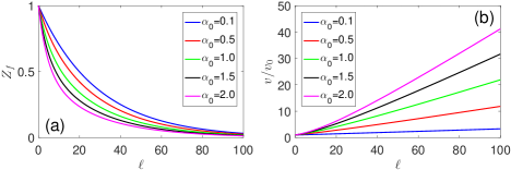
Figure 2: Flowing behavior of $Z_{f}$ and $v$ caused by excitonic fluctuation and Coulomb interaction. In this and all the subsequent figures, we assume $N=2$ in numerical calculations.

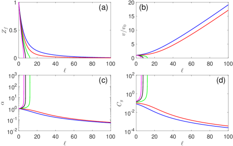
Figure 3: Flowing behavior of $Z_{f}$, $v$, $\alpha$, and $C_{g}$ caused by excitonic fluctuation, Coulomb interaction, and RSP. Blue, red, green, black, and magenta lines correspond to $C_{g0}=0.08,0.1,0.12,0.14,0.16$. Here, $\alpha_{10}=1.0$.

IV.3.1 Isotropic limit

In the isotropic limit with $v_{1}=v_{2}=v$, the RG equations for $Z_{f}$ and $v$ are

$$\frac{dZ_{f}}{d\ell} = \left(-\eta^{A}+C_{0}^{B}-C_{g}\right)Z_{f},$$ (87)

$$\frac{dv}{d\ell} = \left(C^{B}-C_{g}\right)v.$$ (88)

Here, $C^{B}=C_{0}^{B}-C_{1}^{B}=C_{0}-C_{2}^{B}$, in which

$$C_{0}^{B} = \frac{4}{N\pi^{2}}\left[2-\frac{1}{\lambda}\pi+\frac{2-\lambda^{2}}{\lambda}f(\lambda)\right],$$ (89)

$$C_{1,2}^{B} = \frac{4}{N\pi^{2}}\left[1-\frac{1}{\lambda}\frac{\pi}{2}+\frac{1-\lambda^{2}}{\lambda}f(\lambda)\right].$$ (90)

The variable $\lambda$ is $\lambda=N\pi\alpha/4$, and the function $f(\lambda)$ is

$$f(\lambda)=\left\{\begin{array}[]{ll}\frac{1}{\sqrt{1-\lambda^{2}}}\arccos\left(\lambda\right)&\lambda<1\\ \\ \frac{1}{\sqrt{\lambda^{2}-1}}\mathrm{arccosh}\left(\lambda\right)&\lambda>1\\ \\ 1&\lambda=1.\end{array}\right.$$ (96)

In the clean limit, $Z_{f}$ and $v$ flow as follows

$$\frac{dZ_{f}}{d\ell} = \left(-\eta^{A}+C_{0}^{B}\right)Z_{f},$$ (97)

$$\frac{dv}{d\ell} = C^{B}v.$$ (98)

The numerical solutions are shown in Fig. 2. The velocity $v$ increases as the energy is lowered. The Coulomb interaction is marginally irrelevant since its strength parameter $\alpha=e^{2}/v\epsilon$ flows to zero slowly in the lowest energy limit. Both $C_{0}^{B}$ and $C^{B}$ vanish as $\alpha\rightarrow 0$. The velocity renormalization produces logarithmic-like correction to the temperature or energy dependence of some observable quantities, including specific heat and compressibility Kotov12 . The singular renormalization of fermion velocities has been observed by various experimental tools Elias11 ; Siegel11 ; Chae12 ; Yu13 . At low energies, $C_{0}^{B}$ is much smaller than $\eta^{A}$. Thus, the Coulomb interaction only slightly alters the low-energy behavior of $Z_{f}$ induced by the excitonic fluctuation.

For RSP, the RG equation of $C_{g}$ is

$$\frac{dC_{g}}{d\ell}=\left(-2C^{B}+2C_{g}\right)C_{g}.$$ (99)

For a given $\alpha_{0}$, there exists a critical value $C^{B}(\alpha_{0})$. The system exhibits entirely different low-energy properties when $C_{g0}$ is greater and smaller than $C^{B}(\alpha_{0})$. To illustrate this, we show the $\ell$-dependence of $Z_{f}$, $v$, $\alpha$, and $C_{g}$ in Fig. 3. If $C_{g0}<C^{B}(\alpha_{0})$, $Z_{f}$, $\alpha$, and $C_{g}$ all flow to zero as $\ell\rightarrow\infty$, but $v$ increases with growing $\ell$. These results indicate that weak RSP is suppressed by the Coulomb interaction. If $C_{g0}>C^{B}(\alpha_{0})$, both $C_{g}$ and $\alpha$ formally diverge at some finite energy scale, whereas both $Z_{f}$ and $v$ decrease rapidly down to zero at the same energy scale. Thus, strong RSP still drives a NFL-to-CDM transition. As can be seen from the flow diagram presented in Fig. 4(a), the $(\alpha,C_{g})$ plane is divided by the critical line $C_{g0}=C^{B}(\alpha_{0})$ into two distinct phases: the NFL phase and the CDM phase.

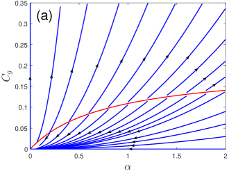
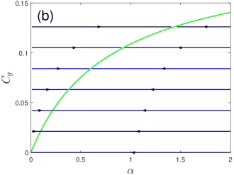
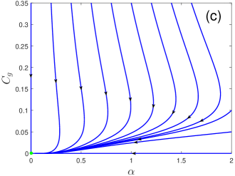
Figure 4: Flowing diagrams on the $\alpha$-$C_{g}$ plane. Result for RSP is in (a), RVP in (b), and RM in (c).

For RVP, the $\ell$-dependence of $Z_{f}$, $v$, $\alpha$, and $C_{g}$ are shown in Fig. 5. The parameter $C_{g}$ does not flow at all, namely

$$\frac{dC_{g}}{d\ell}=0.$$ (100)

We fix $C_{g}$ at a constant: $C_{g}=C_{g0}$. For a given $C_{g0}$, $v$ approaches to a constant value $v^{*}$ in the zero energy limit. The value of $v^{*}$ is obtained from

$$C^{B}(\alpha^{*})=C_{g0},$$ (101)

where $\alpha^{*}=e^{2}/v^{*}\epsilon$. RG analysis indicates that the system always flows to a stable infrared fixed point for any two given initial values of $\alpha$ and $C_{g}$. Connecting all of these fixed points forms a critical line on the $\alpha$-$C_{g}$ plane, as shown in Fig. 4(b). Near the critical line, the specific heat behaves as

$$C_{v}(T)\sim\frac{1}{{v^{*}}^{2}}T^{2}\sim T^{2}.$$ (102)

The residue is

$$Z_{f} \sim e^{\left(-\eta^{A}+C_{0}^{B}(\alpha^{*})-C_{g0}\right)\ell}$$ (103)

$$\sim e^{\left(-\eta^{A}+C_{1}^{B}(\alpha^{*})\right)\ell},$$

where $C_{1}^{B}(\alpha^{*})$ is negative. This $Z_{f}$ flows to zero more quickly than that induced purely by excitonic fluctuation. The retarded fermion self-energy is

$$\mathrm{Re}\Sigma^{R}(\omega) \sim \omega^{1-\left(\eta^{A}-C_{1}^{B}(\alpha^{*})\right)},$$ (104)

$$\mathrm{Im}\Sigma^{R}(\omega) \sim \omega^{1-\left(\eta^{A}-C_{1}^{B}(\alpha^{*})\right)}.$$ (105)

The DOS takes the form

$$\rho(\omega)\sim\omega^{1+\eta^{A}-C_{1}^{B}(\alpha^{*})}.$$ (106)

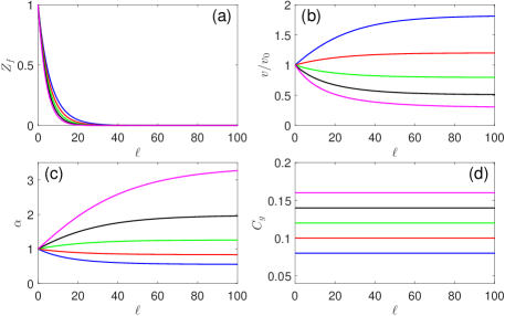
Figure 5: Flowing behavior of $Z_{f}$, $v$, $\alpha$, and $C_{g}$ caused by excitonic fluctuation, Coulomb interaction, and RVP. Blue, red, green, black, and magenta lines correspond to $C_{g0}=0.08,0.1,0.12,0.14,0.16$. Here, $\alpha_{10}=1.0$.

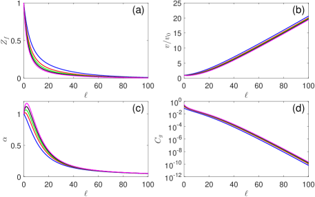
Figure 6: Flowing behavior of $Z_{f}$, $v$, $\alpha$, and $C_{g}$ caused by excitonic fluctuation, Coulomb interaction, and RM. Blue, red, green, black, and magenta lines correspond to $C_{g0}=0.08,0.15,0.2,0.25,0.3$. Here, $\alpha_{10}=1.0$.

For RM, the RG equation for $C_{g}$ is given by

$$\frac{dC_{g}}{d\ell}=\left(-8\eta^{A}+2C^{B}-2C_{g}\right)C_{g}.$$ (107)

The numerical results are plotted in Fig. 6. We observe that $C_{g}$ always approaches to zero quickly, which indicates that RM is irrelevant in the low-energy regime. The Coulomb interaction is marginally irrelevant and leads to singular renormalization of fermion velocity. Accordingly, the DOS and specific heat are

$$\rho(\omega) \sim \frac{\omega^{1+\eta^{A}}}{\ln^{2}(\omega_{0}/\omega)},$$ (108)

$$C_{v}(T) \sim \frac{T^{2}}{\ln^{2}(T_{0}/T)}.$$ (109)

In the presence of RM, the two parameters $(\alpha,C_{g})$ always flow to the stable infrared fixed point $(0,0)$.

Table 1: A summary of low-energy or low-temperature behaviors of some characteristic quantities caused by all the possible combination of the three types of interaction. QFEO stands for the quantum fluctuation of excitonic order parameter. CI represents the Coulomb interaction. We choose to display the $\ell$-dependent quasiparticle residue $Z_{f}(\ell)$, the fermion damping rate $\mathrm{Im}\Sigma^{R}(\omega)$, the DOS $\rho(\omega)$, and the specific heat $C_{v}(T)$. The definitions of all the notations are given in the main text.

Interaction		$Z_{f}(\ell)$	$\mathrm{Im}\Sigma^{R}(\omega)$	$\rho(\omega)$	$C_{v}(T)$
QFEO		$e^{-\eta^{A}\ell}$ Herbut09	$\omega^{1-\eta^{A}}$ Herbut09	$\omega^{1+\eta^{A}}$	$T^{2}$ Herbut09
QFEO+RSP		$e^{-\eta^{A}\ell}\sqrt{1-2C_{g0}\ell}$	$\gamma_{\mathrm{imp}}$	$\gamma_{\mathrm{imp}}\ln(v\Lambda/\gamma_{\mathrm{imp}})$	$\rho(0)T$
QFEO+RVP		$e^{-\left(\eta^{A}+C_{g0}\right)\ell}$	$\omega^{1-\left(\eta^{A}+C_{g0}\right)}$	$\;\omega^{(1-C_{g0})/(1+C_{g0})+\eta^{A}}\;$	$T^{2/(1+C_{g0})}$
QFEO+RM		$e^{-\eta^{A}\ell}$	$\omega^{1-\eta^{A}}$	$\omega^{1+\eta^{A}}$	$T^{2}$
QFEO+CI		$e^{-\eta^{A}\ell}$	$\omega^{1-\eta^{A}}$	$\omega^{1+\eta^{A}}/\ln^{2}(\omega_{0}/\omega)$	$\;T^{2}/\ln^{2}\left(T_{0}/T\right)\;$
QFEO+CI+RSP	$C_{g0}<C_{B}(\alpha_{0})$	$e^{-\eta^{A}\ell}$	$\omega^{1-\eta^{A}}$	$\omega^{1+\eta^{A}}/\ln^{2}(\omega_{0}/\omega)$	$T^{2}/\ln^{2}(T_{0}/T)$
	$C_{g0}>C_{B}(\alpha_{0})$	$\lim_{\ell\rightarrow l_{c}}Z_{f}(\ell)\rightarrow 0$	$\gamma_{\mathrm{imp}}$	$\gamma_{\mathrm{imp}}\ln(v\Lambda/\gamma_{\mathrm{imp}})$	$\rho(0)T$
QFEO+CI+RVP		$e^{\left(-\eta^{A}+C_{1}^{B}(\alpha^{*})\right)\ell}$	$\omega^{1-\left(\eta^{A}-C_{1}^{B}(\alpha^{*})\right)}$	$\omega^{1+\eta^{A}-C_{1}^{B}(\alpha^{*})}$	$T^{2}$
QFEO+CI+RM		$e^{-\eta^{A}\ell}$	$\omega^{1-\eta^{A}}$	$\omega^{1+\eta^{A}}/\ln^{2}(\omega_{0}/\omega)$	$T^{2}/\ln^{2}\left(T_{0}/T\right)$
CI		$\;\lim_{\ell\rightarrow\infty}Z_{f}(\ell)\rightarrow\mathrm{Const.}\;$ Kotov12 ; Gonzalez99 ; Hofmann14 ; WangLiu14	$\omega/\ln^{2}(\omega_{0}/\omega)$ Kotov12 ; WangLiu14	$\omega/\ln^{2}(\omega_{0}/\omega)$ Kotov12 ; WangLiu14	$T^{2}/\ln^{2}(T_{0}/T)$ Kotov12 ; WangLiu14
CI+RSP	$C_{g0}<C_{B}(\alpha_{0})$	$\lim_{\ell\rightarrow\infty}Z_{f}(\ell)\rightarrow\mathrm{Const.}$ WangLiu14	$\omega/\ln^{2}(\omega_{0}/\omega)$ WangLiu14	$\omega/\ln^{2}(\omega_{0}/\omega)$ WangLiu14 ; Stauber05	$T^{2}/\ln^{2}(T_{0}/T)$ WangLiu14 ; Stauber05
	$C_{g0}>C_{B}(\alpha_{0})$	$\lim_{\ell\rightarrow l_{c}}Z_{f}(\ell)\rightarrow 0$ WangLiu14	$\gamma_{\mathrm{imp}}$ Sarma11	$\gamma_{\mathrm{imp}}\ln(v\Lambda/\gamma_{\mathrm{imp}})$ Sarma11	$\rho(0)T$ Sarma11
CI+RVP		$e^{C_{1}^{B}(\alpha^{*})\ell}$ WangLiu14	$\omega^{1+C_{1}^{B}(\alpha^{*})}$ WangLiu14	$\omega^{1-C_{1}^{B}(\alpha^{*})}$ WangLiu14	$T^{2}$ WangLiu14 ; Stauber05 ; Herbut08 ; Vafek08
CI+RM		$e^{C_{1}^{B}(\alpha^{*})\ell}$ WangLiu14	$\omega^{1+C_{1}^{B}(\alpha^{*})}$ WangLiu14	$\omega^{1-C_{1}^{B}(\alpha^{*})}$ WangLiu14	$T^{2}$ WangLiu14 ; Stauber05 ; Herbut08 ; Vafek08

We now compare the quantum critical phenomena to the physical properties of the SM phase. Deep in the SM phase, the excitonic fluctuation can be completely ignored. The low-energy behavior is governed by the interplay of Coulomb interaction and disorder, which has already been extensively investigated WangLiu14 ; Ye98 ; Ye99 ; Stauber05 ; Herbut08 ; Vafek08 ; Foster08 . When the Coulomb interaction and RSP are both present, the system is a normal FL if RSP is weak, but is turned into a CDM phase by strong RSP. Thus, increasing the effective strength of RSP drives a FL-CDM phase transition. In the SM-EI quantum critical regime, increasing the effective strength of RSP leads to a NFL-CDM transition. If RM is added to the system, it is irrelevant around the SM-EI QCP, but is marginal and results in a stable critical line on the $\alpha$-$C_{g}$ plane deep in the SM phase. In contrast, RVP produces the same qualitative low-energy behaviors in the SM phase and around the SM-EI QCP.

We learn from the above analysis that, even if 2D DSM has a gapless SM ground state, the fluctuation of excitonic order parameter gives rise to observable effects at finite $T$ and/or $\omega$. The quantum critical regime can be distinguished from the pure SM phase by measuring the $\omega$-dependence of fermion damping rate and/or the $T$-dependence of specific heat.

To provide a complete analysis of the quantum critical phenomena, we summarize in Table 1 the low-energy properties induced by all the possible combinations of three types of interaction. The quantities presented in Table 1 include the residue $Z_{f}$, damping rate $\mathrm{Im}\Sigma^{R}(\omega)$, fermion DOS $\rho(\omega)$, and specific heat $C_{v}(T)$. We can see that distinct interactions affect each other significantly. The critical phenomena cannot be reliably determined if their mutual influence is not carefully handled.

IV.3.2 Anisotropic case

For different values of fermion velocity ratio, the running behaviors of $Z_{f}$, $v_{1}$, $v_{2}$, and $v_{2}/v_{1}$ obtained in the clean limit are plotted in Figs. 7(a)-(d), respectively. Firstly, $Z_{f}$ flows to zero very quickly, implying the violation of FL description. This is essentially induced by the excitonic quantum fluctuation, because the Coulomb interaction by itself would yield a finite $Z_{f}$. Secondly, the two fermion velocities $v_{1}$ and $v_{2}$ both increase as the energy is lowered, whereas the velocity ratio $v_{2}/v_{1}$ flows to unity in the lowest energy limit. Remember that the excitonic quantum fluctuation does not renormalize fermion velocities at all, as illustrated in Sec. IV.1. It is clear that the renormalization of $v_{1}$ and $v_{2}$ are mainly determined by the Coulomb interaction. These results indicate that both excitonic fluctuation and Coulomb interaction are important in the low-energy region.

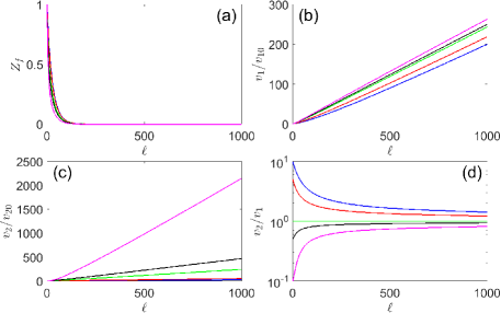
Figure 7: Flowing behavior of $Z_{f}$, $v_{1}$, $v_{2}$, and $v_{2}/v_{1}$ caused by excitonic fluctuation and Coulomb interaction in the anisotropic case. Blue, red, green, black, and magenta lines correspond to $v_{20}/v_{10}=10,5,1,0.5,0.1$. We choose $\alpha_{10}=1.0$. As $\ell\rightarrow\infty$, the system flows to the isotropic limit.

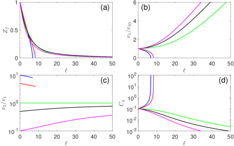
Figure 8: Flowing behavior of $Z_{f}$, $v_{1}$, $v_{2}/v_{1}$, and $C_{g}$ caused by excitonic fluctuation, Coulomb interaction, and RSP. Blue, red, green, black, and magenta lines correspond to $v_{20}/v_{10}=10,5,1,0.5,0.1$. Here, $\alpha_{10}=1.0$ and $C_{g0}=0.1$.

After including three types of disorder, we find that the system still flows to the isotropic limit in the zero energy limit. The numerical results obtained in the cases of RSP, RVP, and RM are presented in Fig. 8, Fig. 9, and Fig. 10, respectively.

First, we consider the case of RSP. As shown in Fig. 8, for given values of $\alpha_{10}$ and $C_{g0}$, $C_{g}$ becomes divergent at some finite energy scale if the bare velocity ratio $v_{20}/v_{10}$ exceeds a critical value. Both $Z_{f}$ and fermion velocities flow to zero at the same energy scale. The anisotropy is suppressed, but the ratio does not flow to the isotropic limit. If the bare value $v_{20}/v_{10}$ is small, $C_{g0}$ flows to zero quickly as the energy is lowered. Meanwhile, the fermion velocities increase, and the ratio $v_{2}/v_{1}\rightarrow 1$. Apparently, the isotropic limit is mainly driven by the Coulomb interaction. The residue $Z_{f}$ still vanishes, owing to the excitonic fluctuation. For given values of $\alpha_{10}$ and $C_{g0}$, varying the velocity ratio $v_{20}/v_{10}$ leads to QPT between CDM phase and NFL phase.

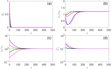
Figure 9: Flowing behavior of $Z_{f}$, $v_{1}$, $v_{2}/v_{1}$, and $C_{g}$ caused by excitonic fluctuation, Coulomb interaction, and RVP. Blue, red, green, black, and magenta lines correspond to $v_{20}/v_{10}=5,2,1,0.5,0.2$. Here, $\alpha_{10}=1.0$, $\Delta/2\pi=0.05$, $v_{\Gamma 10}/v_{10}=1$, and $v_{\Gamma 20}/v_{20}=1$.

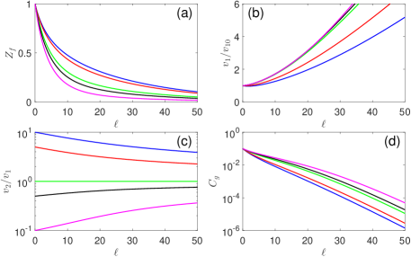
Figure 10: Flowing behavior of $Z_{f}$, $v_{1}$, $v_{2}/v_{1}$, and $C_{g}$ caused by excitonic fluctuation, Coulomb interaction, and RM. Blue, red, green, black, and magenta lines correspond to $v_{20}/v_{10}=10,5,1,0.5,0.1$. Here, $\alpha_{10}=1.0$ and $C_{g0}=0.1$.

In the case of RVP, we show the evolution of $Z_{f}$, $v_{1}$, $v_{2}/v_{1}$, and $C_{g}$ in Fig. 9. Comparing to the clean limit, the ratio $v_{2}/v_{1}$ approaches to unity more quickly. This should be attributed to the fact that the Coulomb interaction strength $\alpha$ flows to certain finite value in the presence of RVP but vanishes in the clean limit. Therefore, the suppression of velocity anisotropy is more significant once RVP is introduced.

We finally turn to the impact of RM. According to Fig. 10, the disorder parameter $C_{g}$ of RM always flows to zero quickly with decreasing energy. The low-energy behaviors of $Z_{f}$ and $v_{1}$ are nearly the same as those obtained in the clean limit, and the velocity ratio $v_{2}/v_{1}\rightarrow 1$ as the energy is lowered down to zero.

V Summary and Discussion

In summary, we have presented a systematic study of the quantum critical phenomena around the SM-EI QCP in 2D DSM. The Yukawa coupling between Dirac fermions and excitonic quantum fluctuation, the long-range Coulomb interaction, and the disorder scattering are treated on equal footing, focusing on their mutual influence and the consequent low-energy properties of the quantum critical regime. We first studied the influence of quantum critical fluctuation of excitonic order parameter, and showed that it invalidates the FL description. We further demonstrated that, adding RSP always drives a NFL-to-CDM transition, and adding RVP further reinforces the NFL behaviors. Nevertheless, adding RM does not change the qualitative results obtained in the clean limit. Once Coulomb interaction is also incorporated, the above results are altered. In particular, the NFL state is protected by the Coulomb interaction for weak RSP, but is eventually replaced by CDM state if RSP is strong enough. When RVP or RM coexist with excitonic fluctuation and Coulomb interaction, the system is in a NFL state. To characterize the NFL and CDM phases, we have calculated several quantities, including the residue, damping rate, fermion DOS, and specific heat. The predicted quantum critical phenomena can be directly probed by experiments.

The results obtained in this paper might be applied to judge whether or not a 2D DSM is close to the SM-EI QCP. Deep in the gapless SM phase, the properties of the system are determined by the combination of Coulomb interaction and disorder. As the system approaches the SM-EI QCP, i.e., $\alpha\rightarrow\alpha_{c}$, the excitonic quantum fluctuation becomes progressively more important, driving the system to enter into the quantum critical regime. Even when the zero-$T$ ground state is gapless, the system could exhibit nontrivial quantum critical behaviors in the $\omega$- and/or $T$-dependence of observable quantities, as illustrated in Fig. 1 and Table 1.

We finally give a brief remark on the existence of the excitonic QCP in realistic graphene. For a 2D DSM, all the previous analytical and numerical calculations CastroNetoPhysics09 ; Khveshchenko01 ; Gorbar02 ; Khveshchenko04 ; Liu09 ; Khveshchenko09 ; Gamayun10 ; Sabio10 ; Zhang11 ; Liu11 ; WangLiu11A ; WangLiu11B ; WangLiu12 ; Popovici13 ; WangLiu14 ; Gonzalez15 ; Carrington16 ; Sharma17 ; Xiao17 ; Carrington18 ; Gamayun09 ; WangJianhui11 ; Katanin16 ; Gonzalez10 ; Gonzalez12 ; Drut09A ; Drut09B ; Drut09C ; Armour10 ; Armour11 ; Buividovich12 ; Ulybyshev13 ; Smith14 ; Juan12 ; Kotikov16 ; Gonzalez14 ; Braguta16 ; Xiao18 have confirmed that an excitonic gap is generated only when $\alpha>\alpha_{c}$, where $\alpha_{c}$ is a nonzero critical value. Recent theoretical studies revealed that the physical value of $\alpha$ in suspendend graphene is not far from the critical value $\alpha_{c}$ Ulybyshev13 ; Carrington18 . The system would become even closer to the excitonic QCP when strain is applied Tang15 ; Sharma17 ; Xiao17 . The organic conductor $\alpha$-(BEDT-TTF)₂I₃, an anisotropic 2D DSM, may also be close to the excitonic QCP Hirata17 . The theoretical results obtained in this work could be utilized to explore the quantum critical phenomena around the putative excitonic QCP in 2D DSM materials.

Appendix A Polarization functions

We now calculate the polarization functions caused by the particle-hole collective excitations. There are two polarization functions, corresponding to the dynamical screening effects of the quantum critical fluctuation of excitonic order parameter and the long-range Coulomb interaction, respectively.

A.1 Polarization function for excitonic fluctuation

For the quantum excitonic fluctuation, the polarization function is defined as

$$\Pi^{A}(\Omega,\mathbf{q}) = N\int\frac{d\omega}{2\pi}\frac{d^{2}\mathbf{k}}{(2\pi)^{2}}\mathrm{Tr}\left[G_{0}(\omega,\mathbf{k})\right.$$ (110)

$$\left.\times G_{0}(\omega+\Omega,\mathbf{k}+\mathbf{q})\right].$$

Substituting the free fermion propagator into Eq. (110), we obtain

$$\Pi^{A}(\Omega,\mathbf{q})=-\frac{4N}{v_{1}v_{2}}\int\frac{d^{3}k}{(2\pi)^{3}}\frac{k\cdot(k+q)}{k^{2}(k+q)^{2}},$$ (111)

where $k=(\omega,\mathbf{k})$. Here, we have employed the following transformations

$$v_{1}k_{1}\rightarrow k_{1},\quad v_{2}k_{2}\rightarrow k_{2},\quad v_{1}q_{1}\rightarrow q_{1},\quad v_{2}q_{2}\rightarrow q_{2}.$$

Using the Feynman parametrization formula

$$\frac{1}{AB}=\int_{0}^{1}dx\frac{1}{[Ax+(1-xB)]^{2}},$$ (113)

one gets

$$\Pi^{A}(\Omega,\mathbf{q}) = -\frac{4N}{v_{1}v_{2}}\int_{0}^{1}dx\int\frac{d^{3}k}{(2\pi)^{3}}$$ (114)

$$\times\frac{k\cdot(k+q)}{\left[(k+xq)^{2}+x(1-x)q^{2}\right]}.$$

Let $k+xq\rightarrow k$, $\Pi_{A}$ can be further written as

$$\Pi^{A}(\Omega,\mathbf{q}) = -\frac{4N}{v_{1}v_{2}}\int^{1}_{0}dx\left\{\int\frac{d^{3}k}{(2\pi)^{3}}\frac{k^{2}}{[k^{2}+x(1-x)q^{2}]^{2}}\right.$$ (115)

$$\left.-\int\frac{d^{3}k}{(2\pi)^{3}}\frac{x(1-x)q^{2}}{[k^{2}+x(1-x)q^{2}]^{2}}\right\}.$$

Performing integration over $k$ by using the standard formula of dimensional regularization

$$\int\frac{d^{d}k}{(2\pi)^{d}}\frac{1}{(k^{2}+\Delta)^{n}} = \frac{1}{(4\pi)^{d/2}}\frac{\Gamma(n-\frac{d}{2})}{\Gamma(n)}\frac{1}{\Delta^{n-\frac{d}{2}}},$$ (116)

$$\int\frac{d^{d}k}{(2\pi)^{d}}\frac{k^{2}}{(k^{2}+\Delta)^{n}} = \frac{1}{(4\pi)^{d/2}}\frac{d}{2}\frac{\Gamma(n-\frac{d}{2}-1)}{\Gamma(n)}\frac{1}{\Delta^{n-\frac{d}{2}-1}},$$

we find that

$$\Pi^{A}(\Omega,\mathbf{q}) = \frac{2N}{v_{1}v_{2}\pi}\sqrt{q^{2}}\int^{1}_{0}dx\sqrt{x(1-x)}$$ (118)

$$= \frac{N}{4v_{1}v_{2}}\sqrt{\Omega^{2}+q_{1}^{2}+q_{2}^{2}}.$$

By taking $q_{1}\rightarrow v_{1}q_{1}$ and $q_{2}\rightarrow v_{2}q_{2}$, we get

$$\Pi^{A}(\Omega,\mathbf{q})=\frac{N}{4v_{1}v_{2}}\sqrt{\Omega^{2}+v_{1}^{2}q_{1}^{2}+v_{2}^{2}q_{2}^{2}}.$$ (119)

A.2 Polarization function for Coulomb interaction

For the Coulomb interaction, the polarization function is given by

$$\Pi^{B}(\Omega,\mathbf{q}) = -N\int\frac{d\omega}{2\pi}\frac{d^{2}\mathbf{k}}{(2\pi)^{2}}\mathrm{Tr}\left[\gamma_{0}G_{0}(\omega,\mathbf{k})\gamma_{0}\right.$$ (120)

$$\left.\times G_{0}(\omega+\Omega,\mathbf{k}+\mathbf{q})\right].$$

Substituting Eq. (6) into Eq. (120) leads to

$$\Pi^{B}(\Omega,\mathbf{q})=\frac{4N}{v_{1}v_{2}}\int\frac{d^{3}k}{(2\pi)^{3}}\frac{2k_{0}(k_{0}+q_{0})-k\cdot(k+q)}{k^{2}(k+q)^{2}}.$$

Making use of the Feynman parametrization formula Eq. (113), along with the transformation $k+xq\rightarrow k$, we recast the above expression as

$$\Pi^{B}(\Omega,\mathbf{q}) = \frac{4N}{v_{1}v_{2}}\int^{1}_{0}dx\left\{\int\frac{d^{3}k}{(2\pi)^{3}}\frac{-k^{2}/3}{[k^{2}+x(1-x)q^{2}]^{2}}\right.$$ (122)

$$\left.+\int\frac{d^{3}k}{(2\pi)^{3}}\frac{x(1-x)\left(q^{2}-2q_{0}^{2}\right)}{[k^{2}+x(1-x)q^{2}]^{2}}\right\}.$$

Repeating the calculational steps that lead to Eq. (119), we finally obtain

$$\Pi^{B}(\Omega,\mathbf{q})=\frac{N}{8v_{1}v_{2}}\frac{v_{1}^{2}q_{1}^{2}+v_{2}^{2}q_{2}^{2}}{\sqrt{\Omega^{2}+v_{1}^{2}q_{1}^{2}+v_{2}^{2}q_{2}^{2}}}.$$ (123)

Appendix B Fermion self-energy

The fermion self-energy corrections come from three sorts of interaction, namely the Yukawa coupling, Coulomb interaction, and disorder scattering. The former two interactions are inelastic, and the third one is elastic. We now calculate them in order.

B.1 Contribution from Yukawa coupling

The fermion self-energy induced by the Yukawa coupling takes the form

$$\Sigma^{A}(\omega,\mathbf{k}) = \int^{\prime}\frac{d\Omega}{2\pi}\frac{d^{2}{\mathbf{q}}}{(2\pi)^{2}}G_{0}(\Omega+\omega,\mathbf{q}+\mathbf{k})D^{A}(\Omega,\mathbf{q})$$ (124)

$$= -\int^{\prime}\frac{d\Omega}{2\pi}\frac{d^{2}{\mathbf{q}}}{(2\pi)^{2}}\frac{\left[-i(\Omega+\omega)\gamma_{0}+v_{1}(q_{1}+k_{1})\gamma_{1}+v_{2}(q_{2}+k_{2})\gamma_{2}\right]}{\left[(\Omega+\omega)^{2}+v_{1}^{2}(q_{1}+k_{1})^{2}+v_{2}^{2}(q_{2}+k_{2})^{2}\right]}D^{A}(\Omega,\mathbf{q}).$$

This self-energy can be expanded in powers of $i\omega$, $v_{1}k_{1}$, and $v_{2}k_{2}$. To the leading order, we get

$$\Sigma^{A}(\omega,\mathbf{k}) = i\omega\gamma_{0}\int^{\prime}\frac{d\Omega}{2\pi}\frac{d^{2}{\mathbf{q}}}{(2\pi)^{2}}\frac{-\Omega^{2}+v_{1}^{2}q_{1}^{2}+v_{2}^{2}q_{2}^{2}}{\left(\Omega^{2}+v_{1}^{2}q_{1}^{2}+v_{2}^{2}q_{2}^{2}\right)^{2}}\frac{1}{\frac{N}{4v_{1}v_{2}}\sqrt{\Omega^{2}+v_{1}^{2}q_{1}^{2}+v_{2}^{2}q_{2}^{2}}}$$ (127)

$$-v_{1}k_{1}\gamma_{1}\int^{\prime}\frac{d\Omega}{2\pi}\frac{d^{2}{\mathbf{q}}}{(2\pi)^{2}}\frac{\Omega^{2}-v_{1}^{2}q_{1}^{2}+v_{2}^{2}q_{2}^{2}}{\left(\Omega^{2}+v_{1}^{2}q_{1}^{2}+v_{2}^{2}q_{2}^{2}\right)^{2}}\frac{1}{\frac{N}{4v_{1}v_{2}}\sqrt{\Omega^{2}+v_{1}^{2}q_{1}^{2}+v_{2}^{2}q_{2}^{2}}}$$

$$-v_{2}k_{2}\gamma_{2}\int^{\prime}\frac{d\Omega}{2\pi}\frac{d^{2}{\mathbf{q}}}{(2\pi)^{2}}\frac{\Omega^{2}+v_{1}^{2}q_{1}^{2}-v_{2}^{2}q_{2}^{2}}{\left(\Omega^{2}+v_{1}^{2}q_{1}^{2}+v_{2}^{2}q_{2}^{2}\right)^{2}}\frac{1}{\frac{N}{4v_{1}v_{2}}\sqrt{\Omega^{2}+v_{1}^{2}q_{1}^{2}+v_{2}^{2}q_{2}^{2}}}.$$

To carry out RG calculation, we choose to integrate over the integral variables within the range

$$\int^{\prime}\frac{d\Omega}{2\pi}\frac{d^{2}{\mathbf{q}}}{(2\pi)^{2}}=\frac{1}{8\pi^{3}}\int_{-\infty}^{+\infty}d\Omega\int_{0}^{2\pi}d\theta\int_{b\Lambda}^{\Lambda}d|\mathbf{q}|\left|\mathbf{q}\right|,$$ (128)

where $b=e^{-\ell}$. It is then easy to obtain

$$\Sigma^{A}(\omega,\mathbf{k})=\left(-i\omega\gamma_{0}C_{0}^{A}+v_{1}k_{1}\gamma_{1}C_{1}^{A}+v_{2}k_{2}\gamma_{2}C_{2}^{A}\right)\ell.$$ (129)

The expressions of $C_{i}^{A}$ are given by Eqs. (25)-(28).

B.2 Contribution from Coulomb interaction

The fermion self-energy induced by the Coulomb interaction is

$$\Sigma^{B}(\omega,\mathbf{k}) = -\int^{\prime}\frac{d\Omega}{2\pi}\frac{d^{2}{\mathbf{q}}}{(2\pi)^{2}}\gamma_{0}G(\Omega+\omega,\mathbf{q}+\mathbf{k})\gamma_{0}D^{B}(\Omega,\mathbf{q})$$ (130)

$$= \int^{\prime}\frac{d\Omega}{2\pi}\frac{d^{2}{\mathbf{q}}}{(2\pi)^{2}}\gamma_{0}\frac{\left[-i(\Omega+\omega)\gamma_{0}+v_{1}(q_{1}+k_{1})\gamma_{1}+v_{2}(q_{2}+k_{2})\gamma_{2}\right]}{\left[(\Omega+\omega)^{2}+v_{1}^{2}(q_{1}+k_{1})^{2}+v_{2}^{2}(q_{2}+k_{2})^{2}\right]}\gamma_{0}D^{B}(\Omega,\mathbf{q}).$$

To the leading order of small energy/momenta expansion, $\Sigma^{B}$ can be approximately written as

$$\Sigma^{B}(\omega,\mathbf{k}) = -i\omega\gamma_{0}\int^{\prime}\frac{d\Omega}{2\pi}\frac{d^{2}{\mathbf{q}}}{(2\pi)^{2}}\frac{-\Omega^{2}+v_{1}^{2}q_{1}^{2}+v_{2}^{2}q_{2}^{2}}{\left(\Omega^{2}+v_{1}^{2}q_{1}^{2}+v_{2}^{2}q_{2}^{2}\right)^{2}}\frac{1}{\frac{|\mathbf{q}|}{\frac{2\pi e^{2}}{\epsilon}}+\frac{N}{8v_{1}v_{2}}\frac{v_{1}^{2}q_{1}^{2}+v_{2}^{2}q_{2}^{2}}{\sqrt{\Omega^{2}+v_{1}^{2}q_{1}^{2}+v_{2}^{2}q_{2}^{2}}}}$$ (131)

$$-v_{1}k_{1}\gamma_{1}\int^{\prime}\frac{d\Omega}{2\pi}\frac{d^{2}{\mathbf{q}}}{(2\pi)^{2}}\frac{\Omega^{2}-v_{1}^{2}q_{1}^{2}+v_{2}^{2}q_{2}^{2}}{\left(\Omega^{2}+v_{1}^{2}q_{1}^{2}+v_{2}^{2}q_{2}^{2}\right)^{2}}\frac{1}{\frac{|\mathbf{q}|}{\frac{2\pi e^{2}}{\epsilon}}+\frac{N}{8v_{1}v_{2}}\frac{v_{1}^{2}q_{1}^{2}+v_{2}^{2}q_{2}^{2}}{\sqrt{\Omega^{2}+v_{1}^{2}q_{1}^{2}+v_{2}^{2}q_{2}^{2}}}}$$

$$-v_{2}k_{2}\gamma_{2}\int^{\prime}\frac{d\Omega}{2\pi}\frac{d^{2}{\mathbf{q}}}{(2\pi)^{2}}\frac{\Omega^{2}+v_{1}^{2}q_{1}^{2}-v_{2}^{2}q_{2}^{2}}{\left(\Omega^{2}+v_{1}^{2}q_{1}^{2}+v_{2}^{2}q_{2}^{2}\right)^{2}}\frac{1}{\frac{|\mathbf{q}|}{\frac{2\pi e^{2}}{\epsilon}}+\frac{N}{8v_{1}v_{2}}\frac{v_{1}^{2}q_{1}^{2}+v_{2}^{2}q_{2}^{2}}{\sqrt{\Omega^{2}+v_{1}^{2}q_{1}^{2}+v_{2}^{2}q_{2}^{2}}}}.$$

Performing integrations according to Eq. (128), we obtain

$$\Sigma^{B}(\omega,\mathbf{k})=\left(-i\omega\gamma_{0}C_{0}^{B}+v_{1}k_{1}\gamma_{1}C_{1}^{B}+v_{2}k_{2}\gamma_{2}C_{2}^{B}\right)\ell.$$ (132)

The expressions of $C_{i}^{B}$ can be found in Eqs. (29)-(32).

B.3 Contribution from disorder scattering

The fermion self-energy generated by disorder is

$$\Sigma_{\mathrm{dis}}(\omega) = \Delta v_{\Gamma}^{2}\int^{\prime}\frac{d^{2}\mathbf{k}}{(2\pi)^{2}}\Gamma G_{0}(\omega,\mathbf{k})\Gamma$$ (133)

$$= i\omega v_{\Gamma}^{2}\Delta\int^{\prime}\frac{d^{2}\mathbf{k}}{(2\pi)^{2}}\frac{\Gamma\gamma_{0}\Gamma}{\left(\omega^{2}+v_{1}^{2}k_{1}^{2}+v_{2}^{2}k_{2}^{2}\right)}$$

$$\approx i\omega\gamma_{0}C_{g}\ell,$$

where

$$C_{g}=\frac{v_{\Gamma}^{2}\Delta}{2\pi v_{1}v_{2}}$$ (134)

for both RSP and RM, and

$$C_{g}=\frac{\left(v_{\Gamma 1}^{2}+v_{\Gamma 2}^{2}\right)\Delta}{2\pi v_{1}v_{2}}$$ (135)

for RVP.

Appendix C Corrections to fermion-disorder coupling

The fermion-disorder coupling receives vertex corrections from three sorts of interaction, including the Yukawa coupling, the Coulomb interaction, and the fermion-disorder interaction, which will be studied below.

C.1 Vertex correction due to Yukawa coupling

The vertex correction due to Yukawa coupling is

$$V^{A}=-\int^{\prime}\frac{d\Omega}{2\pi}\frac{d^{2}\mathbf{q}}{(2\pi)^{2}}G_{0}(\Omega,\mathbf{q})v_{\Gamma}\Gamma G_{0}(\Omega,\mathbf{q})D^{A}(\Omega,\mathbf{q}).$$

For RSP, $\Gamma=\gamma_{0}$ and we get

$$V^{A}=v_{\Gamma}\gamma_{0}\left(-C_{0}^{A}\right)\ell.$$ (137)

For the two components of RVP defined by $\Gamma=\gamma_{1}$ and $\Gamma=\gamma_{2}$, $V_{A}$ is given by

$$V^{A}=v_{\Gamma}\gamma_{1}\left(-C_{1}^{A}\right)\ell,$$ (138)

and

$$V^{A}=v_{\Gamma}\gamma_{2}\left(-C_{2}^{A}\right)\ell,$$ (139)

respectively. For RM with $\Gamma=\mathbbm{1}$, $V_{A}$ is

$$V^{A}=v_{\Gamma}\mathbbm{1}\left(C_{0}^{A}+C_{1}^{A}+C_{2}^{A}\right)\ell.$$ (140)

C.2 Vertex correction due to Coulomb interaction

The vertex correction due to Coulomb interaction is

$$V^{B} = -\int^{\prime}\frac{d\Omega}{2\pi}\frac{d^{2}\mathbf{q}}{(2\pi)^{2}}\gamma_{0}G_{0}(\Omega,\mathbf{q})v_{\Gamma}\Gamma G_{0}(\Omega,\mathbf{q})\gamma_{0}$$ (141)

$$\times D^{B}(\Omega,\mathbf{q}).$$

For RSP with $\Gamma=\gamma_{0}$, $V_{B}$ is

$$V^{B}=v_{\Gamma}\gamma_{0}\left(-C_{0}^{B}\right)\ell.$$ (142)

For the two components of RVP defined by $\Gamma=\gamma_{1}$ and $\Gamma=\gamma_{2}$, we obtain

$$V^{B}=v_{\Gamma}\gamma_{1}\left(-C_{1}^{B}\right)\ell,$$ (143)

and

$$V^{B}=v_{\Gamma}\gamma_{2}\left(-C_{2}^{B}\right)\ell,$$ (144)

respectively. For RM with $\Gamma=\mathbbm{1}$, we find

$$V^{B}=v_{\Gamma}\mathbbm{1}\left(C_{0}^{B}-C_{1}^{B}-C_{2}^{B}\right)\ell.$$ (145)

C.3 Vertex correction from disorder

The vertex correction due to disorder has the form

$$V_{\mathrm{dis}} = \Delta v_{\Gamma}^{2}\int^{\prime}\frac{d^{2}\mathbf{p}}{(2\pi)^{2}}\Gamma G_{0}(0,\mathbf{k})v_{\Gamma}\Gamma G_{0}(0,\mathbf{k})\Gamma$$

$$= v_{\Gamma}\Delta v_{\Gamma}^{2}\int\frac{d^{2}\mathbf{p}}{(2\pi)^{2}}\frac{1}{\left(v_{1}^{2}k_{1}^{2}+v_{2}^{2}k_{2}^{2}\right)^{2}}$$

$$\times\Gamma\left(v_{1}k_{1}\gamma_{1}+v_{2}k_{2}\gamma_{2}\right)\Gamma\left(v_{1}k_{1}\gamma_{1}+v_{2}k_{2}\gamma_{2}\right)\Gamma.$$

For RSP with $\gamma=\gamma_{0}$, $V_{dis}$ is

$$V_{\mathrm{dis}}=v_{\Gamma}\gamma_{0}C_{g}\ell.$$ (147)

For the two components of RVP defined by $\gamma=\gamma_{1}$ and $\gamma_{2}$, $V_{\mathrm{dis}}$ is

$$V_{\mathrm{dis}}=0.$$ (148)

For RM with $\Gamma=\mathbbm{1}$, $V_{\mathrm{dis}}$ is

$$V_{\mathrm{dis}}=-v_{\Gamma}\mathbbm{1}C_{g}\ell.$$ (149)

Appendix D Derivation of the coupled RG equations

The action for the free fermions is given by

$$S_{\Psi} = \sum_{\sigma=1}^{N}\int\frac{d\omega}{2\pi}\frac{d^{2}\mathbf{k}}{(2\pi)^{2}}\bar{\Psi}_{\sigma}(\omega,\mathbf{k})\left(-i\omega\gamma_{0}+v_{1}k_{1}\gamma_{1}+v_{2}k_{2}\gamma_{2}\right)\Psi_{\sigma}(\omega,\mathbf{k}).$$ (150)

Including the fermion self-energies induced by excitonic quantum fluctuation, Coulomb interaction, and disorder scattering, the action of fermions becomes

$$S_{\Psi} = \sum_{\sigma=1}^{N}\int\frac{d\omega}{2\pi}\frac{d^{2}\mathbf{k}}{(2\pi)^{2}}\bar{\Psi}_{\sigma}(\omega,\mathbf{k})\left[-i\omega\gamma_{0}+v_{1}k_{1}\gamma_{1}+v_{2}k_{2}\gamma_{2}-\Sigma^{A}(\omega,\mathbf{k})-\Sigma^{B}(\omega,\mathbf{k})-\Sigma_{\mathrm{dis}}(\omega)\right]\Psi_{\sigma}(\omega,\mathbf{k})$$ (151)

$$\approx \sum_{\sigma=1}^{N}\int\frac{d\omega}{2\pi}\frac{d^{2}\mathbf{k}}{(2\pi)^{2}}\bar{\Psi}_{\sigma}(\omega,\mathbf{k})\left[-i\omega\gamma_{0}e^{\left(-C_{0}^{A}-C_{0}^{B}+C_{g}\right)\ell}+v_{1}k_{1}\gamma_{1}e^{-\left(C_{1}^{A}+C_{1}^{B}\right)\ell}+v_{2}k_{2}\gamma_{2}e^{-\left(C_{2}^{B}+C_{2}^{B}\right)\ell}\right]\Psi_{\sigma}(\omega,\mathbf{k}).$$

Making the following re-scaling transformations:

$$\omega = \omega^{\prime}e^{-\ell},$$ (152)

$$k_{1} = k^{\prime}_{1}e^{-\ell},$$ (153)

$$k_{2} = k^{\prime}_{2}e^{-\ell},$$ (154)

$$\Psi = \Psi^{\prime}e^{\left(2+\frac{C_{0}^{A}}{2}+\frac{C_{0}^{B}}{2}-\frac{C_{g}}{2}\right)\ell},$$ (155)

$$v_{1} = v_{1}^{\prime}e^{\left(-C_{0}^{A}-C_{0}^{B}+C_{1}^{A}+C_{1}^{B}+C_{g}\right)\ell},$$ (156)

$$v_{2} = v_{2}^{\prime}e^{\left(-C_{0}^{A}-C_{0}^{B}+C_{2}^{A}+C_{2}^{B}+C_{g}\right)\ell},$$ (157)

the fermion action is re-written as

$$S_{\Psi^{\prime}}=\sum_{\sigma=1}^{N}\int\frac{d\omega^{\prime}}{2\pi}\frac{d^{2}\mathbf{k}^{\prime}}{(2\pi)^{2}}\bar{\Psi}_{\sigma}^{\prime}(\omega^{\prime},\mathbf{k}^{\prime})\left[-i\omega^{\prime}\gamma_{0}+v_{1}^{\prime}k_{1}^{\prime}\gamma_{1}+v_{2}^{\prime}k_{2}^{\prime}\gamma_{2}\right]\Psi_{\sigma}^{\prime}(\omega^{\prime},\mathbf{k}^{\prime}),$$ (158)

which recovers the form of the original action.

The action for the fermion-disorder coupling is

$$S_{\mathrm{dis}}=\sum_{\sigma=1}^{N}\int\frac{d\omega}{2\pi}\frac{d^{2}\mathbf{k}}{(2\pi)^{2}}\int\frac{d^{2}\mathbf{k}_{1}}{(2\pi)^{2}}\bar{\Psi}_{\sigma}(\omega,\mathbf{k})v_{\Gamma}\Gamma\Psi_{\sigma}(\omega,\mathbf{k}_{1})A(\mathbf{k}-\mathbf{k}_{1})$$ (159)

After taking into account the quantum corrections, it becomes

$$S_{\mathrm{dis}}=\sum_{\sigma=1}^{N}\int\frac{d\omega}{2\pi}\frac{d^{2}\mathbf{k}}{(2\pi)^{2}}\int\frac{d^{2}\mathbf{k}_{1}}{(2\pi)^{2}}\bar{\Psi}_{\sigma}(\omega,\mathbf{k})\left(v_{\Gamma}\Gamma+V^{A}+V^{B}+V_{\mathrm{dis}}\right)\Psi_{\sigma}(\omega,\mathbf{k}_{1})A(\mathbf{k}-\mathbf{k}_{1}).$$ (160)

In the case of RSP, we obtain

$$S_{\mathrm{dis}} = \sum_{\sigma=1}^{N}\int\frac{d\omega}{2\pi}\frac{d^{2}\mathbf{k}}{(2\pi)^{2}}\int\frac{d^{2}\mathbf{k}_{1}}{(2\pi)^{2}}\bar{\Psi}_{\sigma}(\omega,\mathbf{k})\left[v_{\Gamma}\gamma_{0}+v_{\Gamma}\gamma_{0}\left(-C_{0}^{A}\right)\ell+v_{\Gamma}\gamma_{0}\left(-C_{0}^{B}\right)\ell+v_{\Gamma}\gamma_{0}C_{g}\ell\right]\Psi_{\sigma}(\omega,\mathbf{k}_{1})A(\mathbf{k}-\mathbf{k}_{1})$$ (161)

$$\approx \sum_{\sigma=1}^{N}\int\frac{d\omega}{2\pi}\frac{d^{2}\mathbf{k}}{(2\pi)^{2}}\int\frac{d^{2}\mathbf{k}_{1}}{(2\pi)^{2}}\bar{\Psi}_{\sigma}(\omega,\mathbf{k})v_{\Gamma}\gamma_{0}e^{\left(-C_{0}^{A}-C_{0}^{B}+C_{g}\right)\ell}\Psi_{\sigma}(\omega,\mathbf{k}_{1})A(\mathbf{k}-\mathbf{k}_{1}).$$

For the two components of RVP, $S_{\mathrm{dis}}$ is expressed as

$$S_{\mathrm{dis}} = \sum_{\sigma=1}^{N}\int\frac{d\omega}{2\pi}\frac{d^{2}\mathbf{k}}{(2\pi)^{2}}\int\frac{d^{2}\mathbf{k}_{1}}{(2\pi)^{2}}\bar{\Psi}_{\sigma}(\omega,\mathbf{k})\left[v_{\Gamma}\gamma_{1}+v_{\Gamma}\gamma_{1}\left(-C_{1}^{A}\right)\ell+v_{\Gamma}\gamma_{1}\left(-C_{1}^{B}\right)\ell\right]\Psi_{\sigma}(\omega,\mathbf{k}_{1})A(\mathbf{k}-\mathbf{k}_{1})$$ (162)

$$\approx \sum_{\sigma=1}^{N}\int\frac{d\omega}{2\pi}\frac{d^{2}\mathbf{k}}{(2\pi)^{2}}\int\frac{d^{2}\mathbf{k}_{1}}{(2\pi)^{2}}\bar{\Psi}_{\sigma}(\omega,\mathbf{k})v_{\Gamma}\gamma_{1}e^{-\left(C_{1}^{A}+C_{1}^{B}\right)\ell}\Psi_{\sigma}(\omega,\mathbf{k}_{1})A(\mathbf{k}-\mathbf{k}_{1}),$$

and

$$S_{\mathrm{dis}} = \sum_{\sigma=1}^{N}\int\frac{d\omega}{2\pi}\frac{d^{2}\mathbf{k}}{(2\pi)^{2}}\int\frac{d^{2}\mathbf{k}_{1}}{(2\pi)^{2}}\bar{\Psi}_{\sigma}(\omega,\mathbf{k})\left[v_{\Gamma}\gamma_{2}+v_{\Gamma}\gamma_{2}\left(-C_{2}^{A}\right)\ell+v_{\Gamma}\gamma_{2}\left(-C_{2}^{B}\right)\ell\right]\Psi_{\sigma}(\omega,\mathbf{k}_{1})A(\mathbf{k}-\mathbf{k}_{1})$$ (163)

$$\approx \sum_{\sigma=1}^{N}\int\frac{d\omega}{2\pi}\frac{d^{2}\mathbf{k}}{(2\pi)^{2}}\int\frac{d^{2}\mathbf{k}_{1}}{(2\pi)^{2}}\bar{\Psi}_{\sigma}(\omega,\mathbf{k})v_{\Gamma}\gamma_{2}e^{-\left(C_{2}^{A}+C_{2}^{B}\right)\ell}\Psi_{\sigma}(\omega,\mathbf{k}_{1})A(\mathbf{k}-\mathbf{k}_{1}),$$

respectively. For RM, $S_{\mathrm{dis}}$ is cast in the form

$$S_{\mathrm{dis}} = \sum_{\sigma=1}^{N}\int\frac{d\omega}{2\pi}\frac{d^{2}\mathbf{k}}{(2\pi)^{2}}\int\frac{d^{2}\mathbf{k}_{1}}{(2\pi)^{2}}\bar{\Psi}_{\sigma}(\omega,\mathbf{k})\left[v_{\Gamma}\mathbbm{1}+v_{\Gamma}\mathbbm{1}\left(C_{0}^{A}+C_{1}^{A}+C_{2}^{A}\right)\ell+v_{\Gamma}\mathbbm{1}\left(C_{0}^{B}-C_{1}^{B}-C_{2}^{B}\right)\ell-v_{\Gamma}\mathbbm{1}C_{g}\ell\right]$$ (164)

$$\times\Psi_{\sigma}(\omega,\mathbf{k}_{1})A(\mathbf{k}-\mathbf{k}_{1})$$

$$= \sum_{\sigma=1}^{N}\int\frac{d\omega}{2\pi}\frac{d^{2}\mathbf{k}}{(2\pi)^{2}}\int\frac{d^{2}\mathbf{k}_{1}}{(2\pi)^{2}}\bar{\Psi}_{\sigma}(\omega,\mathbf{k})v_{\Gamma}\mathbbm{1}e^{\left(C_{0}^{A}+C_{1}^{A}+C_{2}^{A}+C_{0}^{B}-C_{1}^{B}-C_{2}^{B}-C_{g}\right)\ell}\Psi_{\sigma}(\omega,\mathbf{k}_{1})A(\mathbf{k}-\mathbf{k}_{1}).$$

We then employ the re-scaling transformations given by Eqs. (152)-(155). The random potential $A(\mathbf{k})$ should be re-scaled as follows

$$A(\mathbf{k})=A^{\prime}(\mathbf{k^{\prime}})e^{\ell}.$$ (165)

The parameter $v_{\Gamma}$ is re-scaled as

$$v_{\Gamma}=v_{\Gamma}^{\prime}$$ (166)

for Eq. (161),

$$v_{\Gamma}=v_{\Gamma}^{\prime}e^{\left(-C_{0}^{A}-C_{0}^{B}+C_{1}^{A}+C_{1}^{B}+C_{g}\right)\ell}$$ (167)

for Eq. (162),

$$v_{\Gamma}=v_{\Gamma}^{\prime}e^{\left(-C_{0}^{A}-C_{0}^{B}+C_{2}^{A}+C_{2}^{B}+C_{g}\right)\ell}$$ (168)

for Eq. (163), and

$$v_{\Gamma}=v_{\Gamma}^{\prime}e^{\left(-2C_{0}^{A}-C_{1}^{A}-C_{2}^{A}-2C_{0}^{B}+C_{1}^{B}+C_{2}^{B}+2C_{g}\right)\ell}$$ (169)

for Eq. (164). After carrying out the above manipulations, we re-write the action for fermion-disorder coupling as follows

$$S_{\mathrm{dis}}=\sum_{\sigma=1}^{N}\int\frac{d\omega^{\prime}}{2\pi}\frac{d^{2}\mathbf{k}^{\prime}}{(2\pi)^{2}}\int\frac{d^{2}\mathbf{k}_{1}^{\prime}}{(2\pi)^{2}}\bar{\Psi}_{\sigma}^{\prime}(\omega^{\prime},\mathbf{k}^{\prime})v_{\Gamma}^{\prime}\mathbbm{1}\Psi_{\sigma}^{\prime}(\omega^{\prime},\mathbf{k}_{1}^{\prime})A^{\prime}(\mathbf{k}^{\prime}-\mathbf{k}_{1}^{\prime}),$$ (170)

which restores the form of the original action.

From Eqs. (155), we obtain the RG equation for the quasiparticle $Z_{f}$

$$\frac{dZ_{f}}{d\ell}=\left(C_{0}^{A}+C_{0}^{B}-C_{g}\right)Z_{f}.$$ (171)

According to Eqs. (156) and (157), the RG equations for $v_{1}$ and $v_{2}$ are given by

$$\frac{dv_{1}}{d\ell} = \left(C_{0}^{A}+C_{0}^{B}-C_{1}^{A}-C_{1}^{B}-C_{g}\right)v_{1},$$ (172)

$$\frac{dv_{2}}{d\ell} = \left(C_{0}^{A}+C_{0}^{B}-C_{2}^{A}-C_{2}^{B}-C_{g}\right)v_{2}.$$ (173)

The RG equation for the velocity ratio $v_{2}/v_{1}$ can be readily derived:

$$\frac{d\left(v_{2}/v_{1}\right)}{d\ell} = \frac{\frac{dv_{2}}{dl}v_{1}-v_{2}\frac{dv_{1}}{dl}}{v_{1}^{2}}$$ (174)

$$= \left(C_{1}^{A}-C_{2}^{A}+C_{1}^{B}-C_{2}^{B}\right)\frac{v_{2}}{v_{1}}.$$

Based on Eqs. (166)-(169), we obtain the RG equation for the parameter $v_{\Gamma}$

$$\left\{\begin{array}[]{ll}\frac{dv_{\Gamma}}{d\ell}=0&\texttt{RSP},\\ \\ \frac{dv_{\Gamma}}{d\ell}=\left(C_{0}^{A}+C_{0}^{B}-C_{1}^{A}-C_{1}^{B}-C_{g}\right)v_{\Gamma}&\gamma_{1}\ \texttt{component of RVP}\\ \\ \frac{dv_{\Gamma}}{d\ell}=\left(C_{0}^{A}+C_{0}^{B}-C_{2}^{A}-C_{2}^{B}-C_{g}\right)v_{\Gamma}&\gamma_{2}\ \texttt{component of RVP}\\ \\ \frac{dv_{\Gamma}}{d\ell}=\left(2C_{0}^{A}+C_{1}^{A}+C_{2}^{A}+2C_{0}^{B}-C_{1}^{B}-C_{2}^{B}-2C_{g}\right)v_{\Gamma}&\texttt{RM}\end{array}\right.$$ (182)

References

- (1) S. Das Sarma, S. Adam, E. H. Hwang, and E. Rossi, Rev. Mod. Phys. 83, 407 (2011).
- (2) V. N. Kotov, B. Uchoa, V. M. Pereira, F. Guinea, and A. H. Castro Neto, Rev. Mod. Phys. 84, 1067 (2012).
- (3) O. Vafek and A. Vishwanath, Annu. Rev. Condens. Matter Phys. 5, 83 (2014).
- (4) T. O. Wehling, A. M. Black-Schaffer, and A. V. Balatsky, Adv. Phys. 63, 1 (2014).
- (5) X. Wan, A. M. Turner, A. Vishwanath, and S. Y. Savrasov, Phys. Rev. B 83, 205101 (2011).
- (6) H. Weng, X. Dai, and Z. Fang, J. Phys.: Condens. Matter 28, 303001 (2016).
- (7) C. Fang, H. Weng, X. Dai, and Z. Fang, Chin. Phys. B 25, 117106 (2016).
- (8) B. Yan and C. Felser, Annu. Rev. Condens. Matter Phys. 8, 337 (2017).
- (9) M. Z. Hasan, S.-Y. Xu, I. Belopolski, and S.-M. Huang, Annu. Rev. Condens. Matter Phys. 8, 289 (2017).
- (10) N. P. Armitage, E. J. Mele, and A. Vishwanath, Rev. Mod. Phys. 90, 015001 (2018).
- (11) J. González, F. Guinea, and M. A. H. Vozmediano, Phys. Rev. B 59, R2474(R) (1999).
- (12) J. Hofmann, E. Barnes, and S. Das Sarma, Phys. Rev. Lett. 113, 105502 (2014).
- (13) A. Sharma and P. Kopietz, Phys. Rev. B 93, 235425 (2016).
- (14) P. Goswami and S. Chakravarty, Phys. Rev. Lett. 107, 196803 (2011).
- (15) P. Hosur, S. A. Parameswaran, and A. Vishwanath, Phys. Rev. Lett. 108, 046602 (2012).
- (16) J. Hofmann, E. Barnes, and S. Das Sarma, Phys. Rev. B 92, 045104 (2015).
- (17) R. E. Throckmorton, J. Hofmann, E. Barnes, and S. Das Sarma, Phys. Rev. B 92, 115101 (2015).
- (18) A. Sharma, A. Scammell, J. Krieg, and P. Kopietz, Phys. Rev. B 97, 125113 (2018).
- (19) B.-J. Yang, E.-G. Moon, H. Isobe, and N. Nagaosa, Nat. Phys. 10, 774 (2014).
- (20) A. A. Abrikosov, J. Low. Temp. Phys. 8, 315 (1972).
- (21) A. A. Abrikosov and S. D. Beneslavskii, Sov. Phys. JETP 32, 699 (1971).
- (22) A. A. Abrikosov, Sov. Phys. JETP 39, 709 (1974).
- (23) E.-G. Moon, C. Xu, Y. B. Kim, and L. Balents, Phys. Rev. Lett. 111, 206401 (2013).
- (24) I. F. Herbut and L. Janssen, Phys. Rev. Lett. 113, 106401 (2014).
- (25) L. Janssen and I. F. Herbut, Phys. Rev. B 92, 045117 (2015).
- (26) P. T. Dumitrescu, Phys. Rev. B 92, 121102(R) (2015).
- (27) L. Janssen and I. F. Herbut, Phys. Rev. B 95, 075101 (2017).
- (28) Y. Huh, E.-G. Moon, and Y. B. Kim, Phys. Rev. B 93, 035138 (2016).
- (29) G. Y. Cho and E.-G. Moon, Sci. Rep. 6, 19198 (2016).
- (30) H. Isobe and L. Fu, Phys. Rev. B 93, 241113 (2016).
- (31) H.-H. Lai, Phys. Rev. B 91, 235131 (2015).
- (32) S.-K. Jian and H. Yao, Phys. Rev. B 92, 045121 (2015).
- (33) S.-X. Zhang, S.-K. Jian, and H. Yao, Phys. Rev. B 96, 241111 (2017).
- (34) J.-R. Wang, G.-Z. Liu, and C.-J. Zhang, Phys. Rev. B 96, 165142 (2017).
- (35) R. Shankar, Rev. Mod, Phys. 66, 129 (1994).
- (36) A. H. Castro Neto, Physics 2, 30 (2009).
- (37) D. V. Khveshchenko, Phys. Rev. Lett. 87, 246802 (2001).
- (38) E. V. Gorbar, V. P. Gusynin, V. A. Miransky, and I. A. Shovkovy, Phys. Rev. B 66, 045108 (2002).
- (39) D. V. Khveshchenko and H. Leal, Nucl. Phys. B 687, 323 (2004).
- (40) G.-Z. Liu, W. Li, and G. Cheng, Phys. Rev. B 79, 205429 (2009).
- (41) D. V. Khveshchenko, J. Phys.:Condens. Matter 21, 075303 (2009).
- (42) O. V. Gamayun, E. V. Gorbar, and V. P. Gusynin, Phys. Rev. B 81, 075429 (2010).
- (43) J. Sabio, F. Sols, and F. Guinea, Phys. Rev. B 82, 121413(R) (2010).
- (44) C.-X. Zhang, G.-Z. Liu, and M.-Q. Huang, Phys. Rev. B 83, 115438 (2011).
- (45) G.-Z. Liu and J.-R. Wang, New J. Phys. 13, 033022 (2011).
- (46) J.-R. Wang and G.-Z. Liu, J. Phys. Condens. Matter 23, 155602 (2011).
- (47) J.-R. Wang and G.-Z. Liu, J. Phys. Condens. Matter 23, 345601 (2011).
- (48) J.-R. Wang and G.-Z. Liu, New J. Phys. 14, 043036 (2012).
- (49) C. Popovici, C. S. Fischer, and L. von Smekal, Phys. Rev. B 88, 205429 (2013).
- (50) J.-R. Wang and G.-Z. Liu, Phys. Rev. B 89, 195404 (2014).
- (51) J. González, Phys. Rev. B 92, 125115 (2015).
- (52) M. E. Carrington, C. S. Fischer, L. von Smekal, and M. H. Thoma, Phys. Rev. B 94, 125102 (2016).
- (53) A. Sharma, V. N. Kotov, and A. H. Castro Neto, Phys. Rev. B 95, 235124 (2017).
- (54) H.-X. Xiao, J.-R. Wang, H.-T. Feng, P.-L. Yin, and H.-S. Zong, Phys. Rev. B 96, 155114 (2017).
- (55) M. E. Carrington, C. S. Fischer, L. von Smekal, and M. H. Thoma, Phys. Rev. B 97, 115411 (2018).
- (56) O. V. Gamayun, E. V. Gorbar, and V. P. Gusynin, Phys. Rev. B 80, 165429 (2009).
- (57) J. Wang, H. A. Fertig, G. Murthy, and L. Brey, Phys. Rev. B 83, 035404 (2011).
- (58) A. Katanin, Phys. Rev. B 93, 035132 (2016).
- (59) J. González, Phys. Rev. B 82, 155404 (2010).
- (60) J. González, Phys. Rev. B 85, 085420 (2012).
- (61) J. E. Drut and T. A. Lähde, Phys. Rev. Lett. 102, 026802 (2009).
- (62) J. E. Drut and T. A. Lähde, Phys. Rev. B 79, 165425 (2009).
- (63) J. E. Drut and T. A. Lähde, Phys. Rev. B 79, 241405(R) (2009).
- (64) W. Armour, S. Hands, and C. Strouthos, Phys. Rev. B 81, 125105 (2010).
- (65) W. Armour, S. Hands, and C. Strouthos, Phys. Rev. B 84, 075123 (2011).
- (66) P. V. Buividovich and M. I. Polikarpov, Phys. Rev. B 86, 245117 (2012).
- (67) F. de Juan and H. A. Fertig, Solid State Commun. 152, 1460 (2012).
- (68) M. V. Ulybyshev, P. V. Buividovich, M. I. Katsnelson, and M. I. Polikarpov, Phys. Rev. Lett. 111, 056801 (2013).
- (69) D. Smith and L. von Smekal, Phys. Rev. B 89, 195429 (2014).
- (70) A. V. Kotikov and S. Teber, Phys. Rev. D 94, 114010 (2016).
- (71) J. González, Phys. Rev. B 90, 121107(R) (2014).
- (72) V. V. Braguta, M. I. Katsnelson, A. Y. Kotov, and A. A. Nikolaev, Phys. Rev. B 94, 205147 (2016).
- (73) H.-X. Xiao, J.-R. Wang, G.-Z. Liu, and H.-S. Zong, Phys. Rev. B 97, 155122 (2018).
- (74) L. Janssen and I. F. Herbut, Phys. Rev. B 93, 165109 (2016).
- (75) J.-R. Wang, G.-Z. Liu, and C.-J. Zhang, Phys. Rev. B 95, 075129 (2017).
- (76) L. V. Keldysh and Y. V. Kopaev, Fiz. Tverd. Tela. 6, 2791 (1964).
- (77) D. Jerome, T. M. Rice, and W. Kohn, Phys. Rev. 158, 462 (1967).
- (78) Y. Nambu and G. Jona-Lasinio, Phys. Rev. 122, 345 (1961).
- (79) V. A. Miransky, Dynamical Symmetry Breaking in Quantum Field Theories, (World Scientific, 1994).
- (80) D. C. Elias, R. V. Gorbachev, A. S. Mayorov, S. V. Morozov, A. A. Zhukov, P. Blake, L. A. Ponomarenko, I. V. Grigorieva, K. S. Novoselov, F. Guinea, and A. K. Geim, Nat. Phys. 7, 701 (2011).
- (81) A. S. Mayorov, D. C. Elias, I. S. Mukhin, S. V. Morozov, L. A. Ponomarenko, K. S. Novoselov, A. K. Geim, and R. V. Gorbachev, Nano. Lett. 12, 4629 (2012).
- (82) H.-K. Tang, E. Laksono, J. N. B. Rodrigues, P. Sengupta, F. F. Assaad, and S. Adam, Phys. Rev. Lett. 115, 186602 (2015).
- (83) M. Hirata, K. Ishikawa, G. Matsuno, A. Kobayashi, K. Miyagawa, M. Tamura, C. Berthier, and K. Kanoda, Science 358, 1403 (2017).
- (84) A. W. W. Ludwig, M. P. A. Fisher, R. Shankar, and G. Grinstein, Phys. Rev. B 50, 7526 (1994).
- (85) A. A. Nersesyan, A. M. Tsvelik, and F. Wenger, Nucl. Phys. B 438, 561 (1995).
- (86) A. Altland, B. D. Simons, and M. R. Zirnbauer, Phys. Rep. 359, 283 (2002).
- (87) Y. Huh and S. Sachdev, Phys. Rev. B 78, 064512 (2008).
- (88) C. Xu, Y. Qi, and S. Sachdev, Phys. Rev. B 78, 134507 (2008).
- (89) L. Fritz and S. Sachdev, Phys. Rev. B 80, 144503 (2009).
- (90) J. Wang, G.-Z. Liu, and H. Kleinert, Phys. Rev. B 83, 214503 (2011).
- (91) G.-Z. Liu, J.-R. Wang, and J. Wang, Phys. Rev. B 85, 174525 (2012).
- (92) J.-H. She, M. J. Lawler, and E.-A. Kim, Phys. Rev. B 92, 035112 (2015).
- (93) J.-R. Wang, G.-Z. Liu, and C.-J. Zhang, New. J. Phys. 18, 073023 (2016).
- (94) I. F. Herbut, V. Juričic, and B. Roy, Phys. Rev. B 79, 085116 (2009).
- (95) D. A. Siegel, C.-H. Park, C. Hwang, J. Deslippe, A. V. Fedorov, S. G. Louie, and A. Lanzara, Proc. Natl. Acad. Sci. U.S.A. 108, 11365 (2011).
- (96) J. Chae, S. Jung, A. F. Young, C. R. Dean, L. Wang, Y. Gao, K. Watanabe, T. Taniguchi, J. Hone, K. L. Shepard, P. Kim, N. B. Zhitenev, and J. A. Stroscio, Phys. Rev. Lett. 109, 116802 (2012).
- (97) G. L. Yu, R. Jalil, B. Belle, A. S. Mayorov, P. Blake, F. Schedin, S. V. Morozov, L. A. Ponomarenko, F. Chiappini, S. Wiedmann, U. Zeitler, M. I. Katsnelson, A. K. Geim, K. S. Novoselov, and D. C. Elias, Proc. Natl. Acad. Sci. U.S.A. 110, 3282 (2013).
- (98) J. Ye and S. Sachdev, Phys. Rev. Lett. 80, 5409 (1998).
- (99) J. Ye, Phys. Rev. B 60, 8290 (1999).
- (100) T. Stauber, F. Guinea, and M. A. H. Vozmediano, Phys. Rev. B 71, 041406(R) (2005).
- (101) I. F. Herbut, V. Juričić, and O. Vafek, Phys. Rev. Lett. 100, 046403 (2008).
- (102) O. Vafek and M. J. Case, Phys. Rev. B 77, 033410 (2008).
- (103) M. S. Foster and I. L. Aleiner, Phys. Rev. B 77, 195413 (2008).