Nonlinear $q$-Stokes phenomena for $q$-Painlevé I

Abstract

We consider the asymptotic behaviour of solutions of the first $q$-difference Painlevé equation in the limits $|q|\rightarrow 1$ and $n\rightarrow\infty$. Using asymptotic power series, we describe four families of solutions that contain free parameters hidden beyond-all-orders. These asymptotic solutions exhibit Stokes phenomena, which is typically invisible to classical power series methods. In order to investigate such phenomena we apply exponential asymptotic techniques to obtain mathematical descriptions of the rapid switching behaviour associated with Stokes curves. Through this analysis, we also determine the regions of the complex plane in which the asymptotic behaviour is described by a power series expression, and find that the Stokes curves are described by curves known as $q$-spirals.

1 Introduction

In this paper we study the first $q$-difference Painlevé equation ($\text{$q$-P}_{\text{I}}$)

$$\overline{w}\underline{w}=\frac{1}{w}-\frac{1}{xw^{2}},$$ (1)

where $w=w(x),\overline{w}=w(qx),\underline{w}=w(x/q)$, and $q\in\mathbb{C}$ such that $|q|\neq 0,1$. In particular, we assume that $|q|>1$ and consider (1) under the limits $|q|\rightarrow 1$ and $n\rightarrow\infty$. Equation (1) is part of a class of integrable, second-order nonlinear difference equations known as the discrete Painlevé equations that tend to the ordinary Painlevé equations in the continuum limit. More generally, equation (1) is known as a $q$-difference equation since the evolution of the independent variable $x$ takes the form $x=x_{0}q^{n}$ for some initial $x_{0}$.

Motivated by Boutroux’s study of the first Painlevé equation [7], the asymptotic behaviour of (1) in the limit $|x|\rightarrow\infty$ has been considered in [28, 30]. Joshi [28] showed that there exists a true solution satisfying $w\rightarrow 0$ as $|x|\rightarrow\infty$, which is asymptotic to a divergent series. However, [28] does not describe the Stokes switching behaviour that is typically associated with (divergent) asymptotic series.

In this study we uncover the Stokes behaviour present in the solutions of (1) using exponential asymptotic methods. We first introduce a parameter, $\epsilon$, such that the double limit $|q|\rightarrow 1$ and $n\rightarrow\infty$ is equivalent to $\epsilon\rightarrow 0$. Since we may parametrize $x$ by $x=x_{0}q^{n}$, one possible scaling choice which captures the desired behaviour is $n=s/\epsilon$ and $q=1+\epsilon$. Under this choice of scaling we have $x\sim x_{0}e^{s}+\mathcal{O}(\epsilon)$ as $\epsilon\rightarrow 0$. We note that the large $x$ limit may be obtained if $s$ is taken to be sufficiently large and positive.

Exponential asymptotic techniques for differential-difference equations were developed by King and Chapman [35] in order to study a nonlinear model of atomic lattices based on the works of [48, 13]. The authors of [31, 32] applied the Stokes smoothing technique described in [35] to the first and second discrete Painlevé equations and obtained asymptotic approximations which contain exponentially small contributions. The difference equations considered in [31, 32] are of additive type as the independent variable is of the form $z_{n}=\alpha n+\beta$. Motivated by their work, we extend this to $\text{$q$-P}_{\text{I}}$ in order to study asymptotic solutions of $q$-difference equations which display Stokes phenomena.

We note that there are other exponential asymptotic approaches used to study difference equations [47, 49, 25]. In particular, Olde Daalhuis [47] considered a certain class of second-order linear difference equations, and applied Borel summation techniques in order to obtain asymptotic expansions with exponentially small error. The methods used in these studies involves applying Borel resummation to the divergent asymptotic series of the problem, which allows the optimally-truncated error to be computed directly. We note that Borel summation techniques may be applied whenever a series possess factorial-over-power divergence in the late-order terms and therefore could be applied as an alternative approach to that utilised in the present study.

1.1 Background

General solutions to the Painlevé equations are higher transcendental functions, which cannot be expressed exactly in terms of elementary functions and therefore much of the analytic information regarding their general solutions are very limited. In fact, Nishioka [45] proved that the general solutions of $\text{$q$-P}_{\text{I}}$ are not expressible in terms of solutions of first-order $q$-difference equations.

The discrete Painlevé equations have appeared in areas of physical interest such as in mathematical physics models describing two-dimensional quantum gravity [10, 52, 51, 22, 20, 59]. The basis of these models have origins in orthogonal polynomial theory, in which discrete Painlevé equations have been found to commonly appear [55, 38, 39, 40, 56, 57, 36]. Since the discrete Painlevé equations often arise in many nonlinear models of mathematical physics they are often regarded as defining new nonlinear special functions [15, 26].

Motivated by these applications, much research has gone into the asymptotic study of the (discrete) Painlevé equations. Previous asymptotics studies for the first discrete Painlevé equation have been conducted in [27, 58, 31] where the authors found solutions asymptotically free of poles in the large independent variable limit, which share features with the (tri)-tronqueé solutions of the first Painlevé equation found by Boutroux [7]. Asymptotic solutions have also been found for the so called alternate discrete Painlevé I equation [34, 16].

Extending the work of [31], the authors of [32] also find solutions of the second discrete Painlevé equation ($\text{dP}_{\text{II}}$), which are asymptotically free of poles in some domain of the complex plane containing the positive real axis. This was achieved by rescaling the problem such that the step size of the rescaled difference equation is small in the asymptotic limit. A similar study on $\text{dP}_{\text{II}}$ was also investigated by Shimomura [54]. Shimomura showed that an asymptotic solution of $\text{dP}_{\text{II}}$ which reduces to the tri-tronqueé solution of $\text{P}_{\text{II}}$ can be found by choosing a scaling of $\text{dP}_{\text{II}}$ such that the rescaled equation tends to the second continuous Painlevé equation ($\text{P}_{\text{II}}$) in the limit $n\rightarrow\infty$.

The isomonodromic deformation method has also been used to study the asymptotics for nonlinear difference equations [59, 37, 21, 11]. Using the nonlinear steepest descent method developed by Deift and Zhou [17], the authors of [60] find the asymptotic behaviour of solutions of the fifth discrete Painlevé equation in terms of the solutions of the fifth continuous Painlevé equation.

However, there have been very few asymptotic studies on $q$-Painlevé equations. The asymptotic study of variants of the sixth $q$-Painlevé equation have been investigated by Mano [41] and Joshi and Roffelson [33] using the $q$-analogue of the isomonodromic deformation approach. The first $q$-Painlevé equation has also been investigated in [28, 30]. In particular, Joshi [28] proves the existence of true solutions of (1), which are asymptotic to a divergent asymptotic power series in the limit $|x|\rightarrow\infty$. Such expansions are known to exhibit Stokes phenomena in the complex plane.

Stokes phenomena are generally well understood in the case of linear and nonlinear differential equations [50, 9, 24, 14, 12]. The study of Stokes phenomena have also been investigated for nonlinear difference equations [35], and have been extended to study discrete Painlevé equations [31, 32].

In the continuous theory, Borel summation methods are also used to describe Stokes behaviour by resumming divergent asymptotic series expansions. The $q$-analogues of these methods have also been developed for linear $q$-difference equations [61, 62, 63, 18, 53] in order to describe behaviour known as $q$-Stokes phenomena. These methods have been explicitly applied to certain classes of second-order linear $q$-difference equations by Morita [42, 44, 43] and Ohyama [46].

However, $q$-Stokes phenomenon is unlike classical Stokes phenomenon for differential equations. The notion of $q$-Stokes phenomenon and its differences to classical Stokes phenomenon are detailed in [18, 53]. To the best of our knowledge there have been no corresponding studies for nonlinear $q$-difference equations. The goal of this study is to extend the exponential asymptotic methods used in [35, 31, 32] to $q$-difference equations in order to describe Stokes behaviour present in the asymptotic series expansions.

1.2 Exponential asymptotics and Stokes curves

Conventional asymptotic power series methods fail to capture the presence of exponentially small terms, and therefore these terms are often described as lying beyond-all-orders. In order to investigate such terms, exponential asymptotic methods are used. The underlying principle of these methods is that divergent asymptotic series may be truncated so that the divergent tail, also known as the remainder term, is exponentially small in the asymptotic limit [8]. This is known as an optimally-truncated asymptotic series. Thereafter, the problem can be rescaled in order to directly study the behaviour of these exponentially small remainder terms. This idea was introduced by Berry [3, 4, 5], and Berry and Howls [6], who used these methods to determine the behaviour of special functions such as the Airy function.

The basis of this study uses techniques of exponential asymptotics developed by Olde Daalhuis et al. [48] for linear differential equations, extended by Chapman et al. [13] for application to nonlinear differential equations, and further developed by King and Chapman [35] for nonlinear differential-difference equations. A brief outline of the key steps of the process will be provided here, however more detailed explanation of the methodology may be found in these studies.

In order to optimally truncate an asymptotic series, the general form of the coefficients of the asymptotic series is needed. However, in many cases this is an algebraically intractable problem. Dingle [19] investigated singular perturbation problems and noted that the calculation of successive terms of the asymptotic series involves repeated differentiation of the earlier terms. Hence, the late-order terms, $a_{m}$, of the asymptotic series typically diverge as the ratio between a factorial and an increasing power of some function as $m\rightarrow\infty$. A typical form describing this is given by the expression

$$a_{m}\sim\frac{A\,\Gamma(m+\gamma)}{\chi^{m+\gamma}},$$ (2)

as $m\rightarrow\infty$ where $\Gamma$ is the gamma function defined in [1], while $A$, and $\chi$ are functions of the independent variable which do not depend on $m$, known as the prefactor and singulant respectively. The singulant is subject to the condition that it vanishes at the singular points of the leading order behaviour, ensuring that the singularity is present in all higher-order terms. Chapman et al. [13] noted this behaviour in their investigations and utilize (2) as an ansatz for the late-order terms, which may then be used to optimally truncate the asymptotic expansion.

Following [48] we substitute the optimally-truncated series back into the governing equation and study the exponentially small remainder term. When investigating these terms we will discover two important curves known as Stokes and anti-Stokes curves [2]. Stokes curves are curves on which the switching exponential is maximally subdominant compared to the leading order behaviour. As Stokes curves are crossed, the exponentially small behaviour experiences a smooth, rapid change in value in the neighbourhood of the curve; this is known as Stokes switching. Anti-Stokes curves are curves along which the exponential term switches from being exponentially small to exponentially large (and vice versa). We will use these definitions to determine the locations of the Stokes and anti-Stokes curves in this study.

By studying the switching behaviour of the exponentially small remainder term in the neighbourhood of Stokes curves, it is possible to obtain an expression for the remainder term. The behaviour of the remainder associated with the late-order terms in (2) typically takes the form $\mathcal{S}A\exp(-\chi/\epsilon)$, where $\mathcal{S}$ is a Stokes multiplier that is constant away from Stokes curves, but varies rapidly between constant values as Stokes curves are crossed. From this form, it can be shown that Stokes lines follow curves along which $\chi$ is real and positive, while anti-Stokes lines follow curves along which $\chi$ is imaginary. A more detailed discussion of the behaviour of Stokes curves is given in [2].

1.3 Paper outline

In Section 2, we find two classes of solution behaviour of $\text{$q$-P}_{\text{I}}$, which we refer as Type A and Type B solutions. We also determine the formal series expansions of these solutions, and provide the recurrence relations for the coefficients.

In Section 3, we determine the form of the late-order terms for Type A solutions and use this to determine the Stokes structure of these asymptotic series expansions. We then calculate the behaviours of the exponentially small contributions present in these solutions as Stokes curves are crossed. This is then used to determine the regions in which the asymptotic power series are accurate representations of the dominant asymptotic behaviour.

In Section 4, we consider Type B solutions of $\text{$q$-P}_{\text{I}}$ following the analysis in Section 3. In Section 5 we establish a connection between Type A and B solutions to the vanishing and non-vanishing asymptotic solutions of $\text{$q$-P}_{\text{I}}$ found by Joshi [28]. Finally, we discuss the results and conclusions of the paper in Section 6. Appendices A-D contain detailed calculations needed in Section 3.

2 Asymptotic series expansions

In this section, we expand the solution as a formal power series in the limit $\epsilon\rightarrow 0$, obtain the recurrence relation for the coefficients of the series and deduce the general expression of the late-order terms.

We first rewrite (1) as an additive difference equation by setting $x=x_{0}q^{n}$, which gives

$$w_{n+1}w_{n-1}=\frac{1}{w_{n}}-\frac{1}{x_{0}q^{n}w_{n}^{2}},$$ (3)

where $w_{n}=w(x_{0}q^{n})$. In our analysis, we will introduce a small parameter, $\epsilon$, by rescaling the variables appearing in (3). The choice of scalings we apply are given by

$$s=\epsilon n,\qquad q=1+\epsilon,\qquad w_{n}=W(s).$$ (4)

Under these scalings, equation (3) becomes

$$W(s+\epsilon)W(s)^{2}W(s-\epsilon)=W(s)-\frac{1}{x_{0}(1+\epsilon)^{s/\epsilon}},$$ (5)

and consider the limit $\epsilon\rightarrow 0$. We also note that under the scalings given by (4), the independent variable, $x$, has behaviour described by

$$x=(1+\epsilon)^{s/\epsilon}\sim x_{0}e^{s}+\mathcal{O}(\epsilon),$$ (6)

as $\epsilon\rightarrow 0$. As $e^{s}$ is an entire function, we set $x_{0}=1$ for the remainder of this analysis. It can be shown that equation (5) is invariant under the mapping

$$W\mapsto\lambda W,\quad\text{with}\quad s\mapsto s-\frac{\epsilon\log(\lambda)}{\log(1+\epsilon)}\sim s-\log(\lambda)+\mathcal{O}(\epsilon),$$ (7)

as $\epsilon\rightarrow 0$, and where $\lambda^{3}=1$. We note that this corresponds to the rotational symmetry of (1) found in [28].

We expand the solution, $W(s)$, as an asymptotic power series in $\epsilon$ by writing

$$W(s)\sim\sum_{r=0}^{\infty}\epsilon^{r}W_{r}(s),$$ (8)

as $\epsilon\rightarrow 0$. Substituting (8) into (5) and matching terms of $\mathcal{O}(\epsilon^{r})$ we obtain the nonlinear recurrence relation

$$\sum_{q=0}^{r}\sum_{m=0}^{q}\sum_{k=0}^{m}\frac{(-1)^{k}W_{m-k}^{(k)}}{k!}\sum_{j=0}^{q-m}\frac{W_{q-m-j}^{(j)}}{j!}\sum_{b=0}^{r-q}W_{r-q-b}W_{b}=W_{r}-e^{-s}P_{r}(-s)$$ (9)

for $r\geq 0$ and where the polynomials $P_{n}(s)$ are given by

$$P_{n}(s)=\sum_{r=0}^{n}s^{r}\sum_{k=0}^{r}\frac{(-1)^{r-k}}{(r-k)!}\frac{s_{1}(k+n,k)}{(k+n)!},$$

where $s_{1}(n,k)$ are the Stirling numbers of the first kind [1]. This recurrence relations allows us to calculate $W_{r}$ in terms of the previous coefficients. From (9) we find that the leading order behaviour satisfies

$$W_{0}^{4}=W_{0}-e^{-s}.$$ (10)

Equation (10) is invariant under $s\mapsto s+2\pi i$ as the function $e^{s}$ is $2\pi i$-periodic and hence $W_{0}(s)$ is $2\pi i$-periodic. Furthermore, it will be shown in Section 3.2 that the Stokes switching behaviour of (8) depends on $W_{0}(s)$ to leading order. Hence we restrict our attention the domain, $\mathcal{D}_{0}$, described by

$$\mathcal{D}_{0}=\left\{s\in\mathbb{C}\ |\ \text{Im}(s)\in(-\pi,\pi]\right\}.$$ (11)

We also define the domain, $\mathcal{D}_{k}$, which we call $k^{\text{th}}$-adjacent domain, by

$$\mathcal{D}_{k}=\left\{s\in\mathbb{C}\ |\ \text{Im}(s)\in(-\pi+2k\pi,\pi+2k\pi]\right\}.$$ (12)

As $W_{0}$ satisfies a quartic we therefore have four possible leading order behaviours as $\epsilon\rightarrow 0$. We first define the following

$$A=4\left(\frac{2}{3}\right)^{1/3}e^{-s},\qquad B=9+\sqrt{3}\sqrt{27-256e^{-3s}},\qquad C=2^{1/3}3^{2/3},$$ (13)

and

$$D=\frac{A}{B^{1/3}}+\frac{B^{1/3}}{C}.$$ (14)

Then the four solutions for $W_{0}$ are given by

$$W_{0,1}=-\frac{\sqrt{D}}{2}+\frac{i}{2}\sqrt{D+\frac{2}{\sqrt{D}}},\qquad W_{0,2}=-\frac{\sqrt{D}}{2}-\frac{i}{2}\sqrt{D+\frac{2}{\sqrt{D}}},$$ (15)

and

$$W_{0,3}=\frac{\sqrt{D}}{2}+\frac{1}{2}\sqrt{-D+\frac{2}{\sqrt{D}}},\qquad W_{0,4}=\frac{\sqrt{D}}{2}-\frac{1}{2}\sqrt{-D+\frac{2}{\sqrt{D}}}.$$ (16)

From (15) and (16) it can be shown that

$$W_{0,4}(s)=-\sum_{j=1}^{3}W_{0,j}(s).$$ (17)

Each of the leading order solutions, $W_{0}$, are singular at points for which the argument of the square root term of $B$ is equal to zero. The singularities of $W_{0}$ are given by

$$s_{0}=\frac{1}{3}\left(\log\left(\frac{256}{27}\right)+2ik\pi\right),$$ (18)

where $k\in\mathbb{Z}$. Let us denote the singularities in $\mathcal{D}_{0}$ by

$$s_{0,1}=\frac{1}{3}\left(\log\left(\frac{256}{27}\right)-2i\pi\right),\qquad s_{0,2}=\frac{1}{3}\left(\log\left(\frac{256}{27}\right)+2i\pi\right),\qquad s_{0,3}=\frac{1}{3}\log\left(\frac{256}{27}\right).$$ (19)

Then it can be shown that the local behaviour of $W_{0,j}(s)$ near the singular points (18) is given by

$$W_{0,j}\sim\left(\frac{1}{4}\right)^{1/3}e^{2ij\pi/3}+\left(\frac{1}{8\sqrt{2}}\right)^{1/3}e^{2ij\pi/3}\sqrt{s-s_{0,j}}+\mathcal{O}(s-s_{0,j}),$$ (20)

as $s\rightarrow s_{0,j}$ for $j=1,2,3$. Equation (17) shows that $W_{0,4}(s)$ is the sum of $W_{0,j}(s)$ for $j=1,2,3$, and is therefore singular at the points $s_{0,1},s_{0,2}$ and $s_{0,3}$ in $\mathcal{D}_{0}$.

Two types of leading order behaviours can be characterized by the number of points at which they are singular in $\mathcal{D}_{0}$. In the subsequent analysis, we will refer to solutions with leading order behaviour described by $W_{0,j}$ for $j=1,2,3$ as Type A, while those with leading order behaviour described $W_{0,4}$ as Type B.

In Sections 3.3 and 4.1 we will show that the (anti-) Stokes curves emanate from these singularities. Consequently, the Stokes structure of Type A solutions will be shown to emerge from a single singularity in $\mathcal{D}_{0}$, while Type B solutions will have (anti-) Stokes curves emanating from three singular points in $\mathcal{D}_{0}$. In this sense, Type B solutions will have the most complicated Stokes behaviour due to possible interaction effects between the distinct singularities.

3 Type A Exponential Asymptotics

In this section we will investigate the Stokes phenomena exhibited in Type A solutions with leading order behaviour $W_{0,3}$ as $\epsilon\rightarrow 0$. This is done by first determining the leading order behaviour of the late-order terms, which will allow us to optimally truncate (8) and study the optimally-truncated error. The results for the remaining Type A solutions may be obtained using the symmetry (7).

3.1 Late-order terms

As discussed in Section 1.2, the ansatz for the late-order terms is given by a factorial-over-power form since the determination of $W_{r}$ in (9) involves repeated differentiation. We therefore assume that the coefficients of (8) with $W_{0}=W_{0,3}$ are described by

$$W_{r}(s)\sim\frac{U_{3}(s)\Gamma(r+\gamma_{1})}{\chi_{3}(s)^{r+\gamma_{1}}},$$ (21)

as $r\rightarrow\infty$, where $\chi_{3}(s)$ is the singulant, $U_{3}(s)$ is the prefactor and $\gamma_{1}$ a constant. We substitute (21) into (9) to obtain

$$2W_{0,3}^{3}W_{r}+W_{0,3}^{3}\sum_{k=0}^{r}\frac{\left((-1)^{k}+1\right)}{k!}(-\chi_{3}^{\prime})^{k}W_{r}+6W_{0,3}^{2}W_{1}W_{r-1}$$

$$+W_{0,3}^{3}\sum_{k=0}^{r}\frac{\left((-1)^{k}+1\right)}{k!}\left(\binom{k}{1}(-\chi_{3}^{\prime})^{k-1}\frac{U_{3}^{\prime}}{U_{3}}+\binom{k}{2}(-\chi_{3}^{\prime})^{k-2}(-\chi_{3}^{\prime\prime})\right)W_{r-1}$$

$$+\sum_{k=0}^{r-1}\frac{\left((-1)^{k}+1\right)}{k!}(-\chi_{3}^{\prime})^{k}\left(3W_{0,3}^{2}W_{1}+W_{0,3}^{2}W_{0,3}^{\prime}\right)W_{r-1}+\mathcal{O}(W_{r-2})=W_{r}+\cdots,$$ (22)

where the remaining terms are negligible for the purposes of this demonstration as $r\rightarrow\infty$. By matching terms of $\mathcal{O}(W_{r})$ as $r\rightarrow\infty$, we find that the leading order equation is given by

$$2W_{0,3}^{3}+W_{0,3}^{2}\sum_{k=0}^{r}\frac{\left((-1)^{k}+1\right)}{k!}(-\chi_{3}^{\prime})^{k}=1,$$ (23)

as $r\rightarrow\infty$. Matching at the next subsequent order involves matching terms of $\mathcal{O}(W_{r-1})$ in (22). Doing so gives

$$W_{0,3}^{3} \sum_{k=0}^{r}\frac{\left((-1)^{k}+1\right)}{k!}\left(\binom{k}{1}(-\chi_{3}^{\prime})^{k-1}\frac{U_{3}^{\prime}}{U_{3}}+\binom{k}{2}(-\chi_{3}^{\prime})^{k-2}(-\chi_{3}^{\prime\prime})\right)+6W_{0,3}^{2}W_{1}$$

$$+3W_{0,3}^{2}W_{1}\sum_{k=0}^{r-1}\frac{\left((-1)^{k}+1\right)}{k!}(-\chi^{\prime})^{k}+W_{0,3}^{2}W_{0,3}^{\prime}\sum_{k=0}^{r-1}\frac{\left((-1)^{k}-1\right)}{k!}(-\chi_{3}^{\prime})^{k}=0.$$ (24)

as $r\rightarrow\infty$. In order to determine the singulant, $\chi_{3}(s)$, we consider (23). The leading order behaviour of $\chi_{3}(s)$ may be determined by replacing the upper limit of the sum in (23) by infinity. Taking the series to be infinite introduces error in the singulant behaviour which is exponentially small in the limit $r\rightarrow\infty$, which is negligible here [35, 31, 32]. Evaluating the sum appearing in (23) as an infinite series gives

$$\cosh(-\chi_{3}^{\prime})=\frac{1-2W_{0,3}^{3}}{2W_{0,3}^{3}},\quad\chi(s_{0,3})=0.$$ (25)

The solution of (25) is given by

$$\chi_{3}(s;M)=\pm\int_{s_{0,3}}^{s}\left(\cosh(\sigma(t))+2iM\pi\right)\ dt,\qquad\sigma(s)=\frac{1-2W_{0,3}(s)^{3}}{2W_{0,3}(s)^{3}}$$ (26)

where $M\in\mathbb{Z}$. Noting that there are two different expressions for the singulant, we name them $\chi_{3}(s;M)$ and $\chi_{3}^{-}(s;M)$ with the choice of the positive and negative signs respectively. In general, the behaviour of $W_{r}$ will be the sum of expressions (21), with each value of $M$ and sign of the singulant [19]. However, this sum will be dominated by the two terms associated with $M=0$ as this is the value for which $|\chi|$ is smallest [13]. Thus, we consider the $M=0$ case in the subsequent analysis. Hence we set

$$\chi_{3}(s)=\int_{s_{0,3}}^{s}\cosh^{-1}(\sigma(t))dt,\qquad\chi_{3}^{-}(s)=-\int_{s_{0,3}}^{s}\cosh^{-1}(\sigma(t))dt.$$ (27)

In order to determine the prefactor associated with each singulant we solve (3.1). As before, we replace the upper limit of the sum appearing in (3.1) by infinity and use (26) in order to obtain

$$-2W_{0,3}^{3}\sinh(\chi^{\prime})\frac{U_{3}^{\prime}}{U_{3}}-W_{0,3}^{3}\chi_{3}^{\prime\prime}\cosh(\chi_{3}^{\prime})+2W_{0,3}^{2}W_{0,3}^{\prime}\sinh(\chi_{3}^{\prime})+3\frac{W_{1}}{W_{0,3}}=0.$$ (28)

It can be verified that

$$F(s)=\frac{\Upsilon W_{0,3}}{\sqrt{\sinh(\chi_{3}^{\prime})}},$$ (29)

where $\Upsilon$ is a constant of integration, solves the differential equation (28) without the $3W_{1}/W_{0,3}$ term. By setting $U_{3}(s)=F(s)\phi(s)$ and substituting this into (28) we obtain the differential equation

$$\frac{\phi^{\prime}}{\phi}=-\frac{W_{1}\chi_{3}^{\prime\prime}}{W_{0,3}^{\prime}},$$ (30)

where we have used (25) in order to express (30) in terms of $\chi_{3}^{\prime\prime}$. Integrating (30) then gives

$$\phi(s)=\tilde{\Upsilon}\exp\left(-\int^{s}\frac{W_{1}(t)\chi_{3}^{\prime\prime}(t)}{W_{0,3}^{\prime}(t)}dt\right),$$ (31)

where $\tilde{\Upsilon}$ is a constant of integration. Hence, if we let $U_{3}$ and $U_{3}^{-}$ denote the prefactors associated with the singulants $\chi_{3}$ and $\chi_{3}^{-}$, respectively, then the solutions of (28) are given by

$$U_{3}(s)=\frac{\Lambda W_{0,3}e^{-G}}{\sqrt{\sinh(\chi_{3}^{\prime})}},\qquad U_{3}^{-}(s)=\frac{\tilde{\Lambda}W_{0,3}e^{G}}{\sqrt{\sinh(\chi_{3}^{\prime})}},$$ (32)

where $\Lambda,\tilde{\Lambda}$ are constants (which depend on $\Upsilon$ and $\tilde{\Upsilon}$) and

$$G(s)=\int^{s}\frac{W_{1}(t)\chi_{3}^{\prime\prime}(t)}{W_{0,3}^{\prime}(t)}dt.$$ (33)

Substituting the (27) and (32) into (21) shows that

$$W_{r}(s)\sim\frac{W_{0,3}\Gamma(r+\gamma_{1})}{\sqrt{\sinh(\chi_{3}^{\prime})}\chi_{3}^{r+\gamma_{1}}}\left(\Lambda e^{-G}+\frac{\tilde{\Lambda}e^{G}}{(-1)^{r+\gamma_{1}}}\right),$$ (34)

as $r\rightarrow\infty$.

To completely determine the form of the $W_{r}$ we must also determine the value of $\gamma_{1}$. This requires matching the late-order expression given in (21) to the leading-order behaviour in the neighbourhood of the singularity. This procedure is described in Appendix B, and shows that $\gamma_{1}=-1/2$ and $\tilde{\Lambda}=-i\Lambda$.

From the results obtained in Appendix B, we find that

$$W_{2r}(s)\sim\frac{2W_{0,3}\Lambda\cosh(G)\Gamma(2r-1/2)}{\sqrt{\sinh(\chi_{3}^{\prime})}\chi_{3}^{2r-1/2}},\qquad W_{2r+1}(s)\sim-\frac{2W_{0,3}\Lambda\sinh(G)\Gamma(2r+1/2)}{\sqrt{\sinh(\chi_{3}^{\prime})}\chi_{3}^{2r+1/2}},$$ (35)

as $r\rightarrow\infty$. Hence, (35) reveals that the asymptotic series (8) may be expressed as the sum of two asymptotic series in even and odd powers of $\epsilon$.

In the following analysis, we apply optimal truncation methods to the asymptotic series, (8) and show that the optimal truncation error is proportional to $U_{3}e^{-\chi_{3}/\epsilon}$.

3.2 Stokes smoothing

In order to determine the behaviour of the exponentially small contributions in the neighbourhood of the Stokes curve we optimally truncate (8). We truncate the asymptotic series at the least even term by writing

$$W(s)=\sum_{r=0}^{2N_{\text{opt}}-1}\epsilon^{r}W_{r}(s)+R_{N}(s),$$ (36)

where $N_{\text{opt}}$ is the optimal truncation point and $R_{N}$ is the optimally-truncated error. As the analysis is technical, we will summarize the key results in this section with the details provided in Appendix C.

In Appendix C, we show that the optimal truncation point is given by $N_{\text{opt}}\sim(|\chi_{3}|/\epsilon+\kappa)/2,$ as $\epsilon\rightarrow 0$, and where $\kappa\in[0,1)$ is chosen such that $N_{\text{opt}}\in\mathbb{Z}$.

The leading order behaviour of the remainder term in the small $\epsilon$ limit can be shown to take the form

$$R_{N}\sim\mathcal{S}_{3}U_{3}e^{-\chi_{3}/\epsilon},$$ (37)

where $\mathcal{S}_{3}$ is the Stokes switching parameter which varies rapidly between constant values in the neighbourhood of Stokes curves.

For algebraic convenience, we let $T(s)$ represent the finite sum in (36) and use the shift notation denoted by $F=F(s),\overline{F}=F(s+\epsilon),\underline{F}=F(s-\epsilon)$. By substituting the truncated series, (36), into the governing equation (5) we obtain

$$T^{2}\underline{T}\overline{R}+2\overline{T}T\underline{T}R+\overline{T}T^{2}\underline{R}+\epsilon^{2N}(W_{2N}-4W_{0,3}^{3}W_{2N})+\cdots=R,$$ (38)

where the terms neglected are of order $\mathcal{O}(\epsilon^{2N+1}W_{2N+1})$ and quadratic in $R_{N}$. Terms of these sizes are negligible compared to the terms kept in (38) as $\epsilon\rightarrow 0$.

Recall that Stokes switching occurs across Stokes curves, which are characterized by $\text{Im}(\chi)=0$ and $\text{Re}(\chi)>0$. We define the value of the Stokes multiplier, $\mathcal{S}_{3}$, to be

$$\mathcal{S}_{3}=\begin{cases}\mathcal{S}_{3}^{+},\quad\text{in the regions where Im$(\chi)_{3}>0$ and Re$(\chi_{3})>0$,}\\ \mathcal{S}_{3}^{-},\quad\text{in the regions where Im$(\chi)_{3}<0$ and Re$(\chi_{3})>0$.}\end{cases}$$ (39)

In Appendix C we show that the Stokes multiplier, $\mathcal{S}_{3}$, changes in value by

$$\Delta\mathcal{S}_{3}=\mathcal{S}_{3}^{+}-\mathcal{S}_{3}^{-}\sim i\sqrt{2\pi\epsilon}H(\left|\chi_{3}\right|)\int_{-\infty}^{\infty}e^{-x^{2}/2}dx=2i\pi\sqrt{\epsilon}H(\left|\chi_{3}\right|),$$

as Stokes curves are crossed and $H$ is the function defined by $H(\chi_{3}^{\prime})=(1-4W_{0,3}^{3})^{1/2}/\chi_{3}^{\prime}$. Let $\mathcal{S}_{j}$ denote the Stokes multiplier associated with $\chi_{j}$ to be

$$\mathcal{S}_{j}=i\pi\sqrt{\epsilon}H(\left|\chi_{j}\right|)\left(\text{erf}\left(\theta\sqrt{\frac{\left|\chi_{j}\right|}{2\epsilon}}\right)+C_{j}\right),$$ (40)

for $j=1,2,3$ and $C_{j}$ is an arbitrary constant. Then the asymptotic power series expansion of Type A solutions of (5) with leading order behaviour, $W_{0,3}$, up to exponentially small corrections is given by

$$W(s)\sim W_{0,3}(s)+\sum_{r=1}^{2N-1}\epsilon^{2r}W_{r}(s)+\mathcal{S}_{3}(s)U_{3}(s)e^{-\chi_{3}(s)/\epsilon},$$ (41)

as $\epsilon\rightarrow 0$. By using the symmetry given by (7) we find that the other Type A solutions are given by

$$W(s) \sim W_{0,1}(s)+\lambda_{1}\sum_{r=1}^{2N-1}\epsilon^{2r}W_{2r}(s)+\mathcal{S}_{1}(s)U_{1}(s)e^{-\chi_{1}(s)/\epsilon},$$ (42)

$$W(s) \sim W_{0,2}(s)+\lambda_{2}\sum_{r=1}^{2N-1}\epsilon^{2r}W_{2r}(s)+\mathcal{S}_{2}(s)U_{2}(s)e^{-\chi_{2}(s)/\epsilon},$$ (43)

as $\epsilon\rightarrow 0$, where $\mathcal{S}_{j}$ is given by (40), $\lambda_{1}=e^{-2i\pi/3}$, $\lambda_{2}=e^{2i\pi/3}$ and

$$\chi_{1}(s)=\chi_{3}(s+2i\pi/3),\quad U_{1}(s)=U_{3}(s+2i\pi/3),\quad\chi_{2}(s)=\chi_{3}(s-2i\pi/3),\quad U_{2}(s)=U_{3}(s-2i\pi/3).$$

In particular, the values of $\Lambda_{j}$ are

$$\Lambda_{1}=\lambda_{1}\Lambda_{3}=e^{-2i\pi/3}\Lambda_{3},\qquad\Lambda_{2}=\lambda_{2}\Lambda_{3}=e^{-2i\pi/3}\Lambda_{3},$$

where $\Lambda_{3}$ is given by (66). Furthermore, the complete asymptotic series expansions of Type A solutions of (5) have Stokes multipliers which contain a free parameter in the form of $C_{j}$. This will be further explained in Section 3.3.

We have successfully determined a family of asymptotic solutions of (5) which contains exponentially small error. These exponentially small terms exhibit Stokes switching and therefore the expressions (41)-(43) describe the asymptotic behaviour in certain regions of the complex plane. The regions of validity for Type A solutions will be determined in Section 3.3.

3.3 Stokes structure

In this section we determine the Stokes structure of Type A solutions in both the complex $s$ and $x$-planes. As demonstrated in Section 3.2, we found that the exponential contributions present in the series expansions (41), (42) and (43) are proportional to $\exp(-\chi_{j}/\epsilon)$. These terms are exponentially small when $\text{Re}(\chi_{j})>0$ and exponentially large when $\text{Re}(\chi_{j})<0$. Hence, by considering (27) we may determine the behaviour of these terms and the location of the (anti-) Stokes curves. Once the Stokes structure has been determined in the complex $s$-plane, we may reverse the scalings given by (4) in order to determine the Stokes structure in the complex $x$-plane.

We first illustrate and explain the Stokes structure and Stokes switching behaviour of (41) in the domain $\mathcal{D}_{0}$, described by (11). The upper and lower boundaries of $\mathcal{D}_{0}$ are described by the curves $\text{Im}(s)=\pm\pi$ and are denoted by the dot-dashed curves in Figure 1(a). In this figure we also see that there are two Stokes curves (red curves) and three anti-Stokes curves (dashed blue curves) emanating from the singularity $s_{0,3}$. The Stokes curves extending towards the upper boundary of $\mathcal{D}_{0}$ switches the exponential contribution associated with $\chi_{3}$ as $\text{Re}(\chi_{3})>0$. This Stokes curve is denoted by ➂ in Figure 1(b). While the Stokes curve extending towards the lower boundary of $\mathcal{D}_{0}$ does not switch any exponential contributions as $\text{Re}(\chi_{3})<0$. Additionally, there is a branch cut (zig-zag curve) of $\chi_{3}$ located along the negative real $s$ axis emanating from $s_{0,3}$. Using this knowledge, we can determine the switching behaviour as Stokes curves are crossed. Additionally, we observe in Figure 1(a) that the (anti-) Stokes curves and the branch cut separate $\mathcal{D}_{0}$ into six regions.

(a) Behaviour of $\chi_{3}$. (b) Exponential behaviour.

Figure 3.1: These figures illustrate the Stokes structure for the Type A solution described by (41) of (5) in $\mathcal{D}_{0}$. Figure 1(a) illustrates the behaviour of $\chi_{3}$ as Stokes and anti-Stokes curves are crossed. Figure 1(b) illustrates regions of $\mathcal{D}_{0}$ in which the exponential contribution associated with $\chi_{3}$ is exponentially large or small. The legend of this figure will apply to all subsequent figures unless stated otherwise.

We now determine regions in $\mathcal{D}_{0}$ in which the asymptotic behaviour of (5) is described by the power series expansion (41), referred to as regions of validity. From Figure 1(a) we observe that the exponential contribution associated with $\chi_{3}$ is exponentially small in the neighbourhood of the upper Stokes curves since $\text{Re}(\chi_{3})>0$, and therefore the presence of $\exp(-\chi_{3}/\epsilon)$ does not affect the dominance of the leading order behaviour in (41). Hence, the value of the Stokes multiplier, $\mathcal{S}_{3}$, in the neighbourhood of the upper Stokes curve may be freely specified, and will therefore contain a free parameter hidden beyond-all-orders. The values of $\mathcal{S}_{3}$ in the regions of $\mathcal{D}_{0}$ is illustrated in Figure 2(a).

The remainder term associated with $\chi_{3}$ will exhibit Stokes switching and therefore the value of $\mathcal{S}_{3}$ varies as it crosses a Stokes curve, say, from state 1 to state 2. Using the naming convention

(a) General values of $\mathcal{S}_{3}$. (b) Regions of validity.

Figure 3.2: Figure 2(a) illustrates the value $\mathcal{S}_{3}$, which is defined by (40) and (39), as Stokes curves are crossed. Figure 2(b) illustrates the regions of validity of the asymptotic solution described by (41). The dark and light grey shaded regions denote regions in which the exponential contribution associated with $\chi_{3}$ is large and small respectively. Hence, the regions of validity are those which are shaded in light grey.

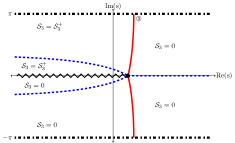
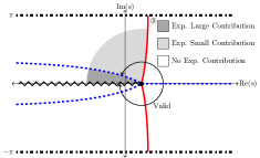
(a) Special values of $\mathcal{S}_{3}$. (b) Extended regions of validity.

Figure 3.3: Figures 3(a) and 3(b) correspond to those in Figure 3.2 for the choice of $\mathcal{S}^{-}_{3}=0$. This specific choice gives an asymptotic solution of (5) with an extended region of validity. Non-shaded regions denote regions in which there are no exponential contributions present. The legend in this figure will be used throughout the remainder of this study, unless stated otherwise.

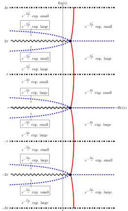
(c) Stokes structure of $\chi_{3}$ in the domains $\mathcal{D}_{0}$, $\mathcal{D}_{1}$ and $\mathcal{D}_{-1}$.

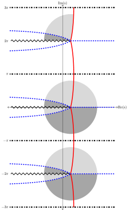
(d) Exponential contributions originating from the domains $\mathcal{D}_{0}$, $\mathcal{D}_{1}$ and $\mathcal{D}_{-1}$.

Figure 3.4: This figure illustrates the Stokes structure depicted in Figure 1(b) extended to the adjacent domains $\mathcal{D}_{1}$ and $\mathcal{D}_{-1}$ as described by (12). In fact, the Stokes structure in the $k^{\text{th}}$-adjacent domains are identical to those in $\mathcal{D}_{0}$ since $W_{0}$ is $2\pi i$-periodic. Each adjacent domain contributes an exponential contribution to the asymptotic solution described by (41). From figure 3.4, we see that the presence of the exponential contribution from $\mathcal{D}_{-1}$ does not affect the dominance of (41) in $\mathcal{D}_{0}$ and hence its associated Stokes multiplier may be freely specified. However, the presence of the exponential contribution from $\mathcal{D}_{1}$ dominates the asymptotic solution, (41). In order for (41) to remain valid in $\mathcal{D}_{0}$, we require the value of the Stokes multiplier associated with exponential contribution in $\mathcal{D}_{1}$ must be chosen to be equal to zero. Figure 3.4 illustrates the regions where each exponential contribution are present.

described by (39), we denote these states by $\mathcal{S}^{-}_{3}$ and $\mathcal{S}^{+}_{3}$ respectively. If we assume that the value of $\mathcal{S}_{3}$ is nonzero on either side of the upper Stokes curve, then we conclude that the exponentially small contribution associated with $\chi_{3}$ is present in the regions bounded by the upper anti-Stokes curve, the anti-Stokes curve emanating from the singularity along the positive real $s$-axis and the curve $\text{Im}(s)=\pi$. Furthermore, the exponential contribution associated with $\chi_{3}$ is also exponentially small in the region bounded by the branch cut and the lower anti-Stokes curve. The regions of validity of the asymptotic solution described by (41) are illustrated in Figure 2(b).

However, for special choices of the free parameter hidden beyond-all-orders, we can obtain asymptotic solutions with an extended range of validity in $\mathcal{D}_{0}$. If we specify the value of $\mathcal{S}^{-}_{3}$ to be equal to zero, then the exponential contribution associated with $\chi_{3}$ is no longer present in regions where it is normally exponentially large. In this case, the region of validity is extended by two additional adjacent sectorial regions in $\mathcal{D}_{0}$ as illustrated in Figure 3(b). We note that the case where $\mathcal{S}^{+}_{3}=0$ is specified can also give Type A solutions with an extended region of validity. However, this only extends the regions of validity of (41) by one additional sectorial region. In both cases the value of $\mathcal{S}_{3}$ is specified, and therefore the asymptotic solution described by (41) is uniquely determined; we call these special Type A asymptotic solutions.

Figure 3.4 illustrates the Stokes structure in the adjacent domains $\mathcal{D}_{1}$ and $\mathcal{D}_{-1}$ as described by (12). Due to the $2\pi i$-periodic nature of $W_{0}$, the Stokes structure is also $2\pi i$-periodic as shown in Figure 3.4. Hence, we obtain an exponential contribution in each adjacent domain $\mathcal{D}_{k}$. For integers $k\leq-1$, there are exponentially small contributions present in the adjacent domains $\mathcal{D}_{k}$. The presence of these exponentially small contributions do not affect the asymptotic behaviour in the principal domain, $\mathcal{D}_{0}$ and hence the corresponding Stokes multipliers may be freely specified. However, for integers $k\geq 1$

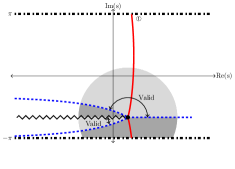
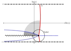
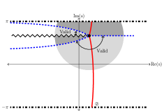
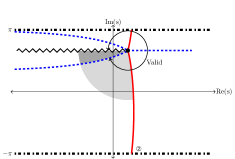
(a) Regions of validity for the asymptotic solution described by (42). (b) Extended regions of validity for the asymptotic solution described by (42). (c) Regions of validity for the asymptotic solution described by (43). (d) Extended regions of validity for the asymptotic solution described by (43).

Figure 3.5: This figure illustrates the Stokes structure and regions of validity for the remaining two Type A solutions. We observe that these Stokes structures are vertical translations of those illustrated in Figure 3.1, which is due to the symmetry described by (7). Figures 5(a) and 5(b) illustrate the regions of validity for the general and special asymptotic solution described by (42). Figures 5(c) and 5(d) illustrate the regions of validity for the general and special asymptotic solution described by (43).

the exponential contributions originating from the adjacent domains $\mathcal{D}_{k}$ do affect the asymptotic behaviour in $\mathcal{D}_{0}$. In order for the asymptotic solution (41) to correctly describe the solution behaviour in $\mathcal{D}_{0}$, the value of the Stokes multipliers must be specified such that the are not present in $\mathcal{D}_{0}$. The presence of the exponential contributions in the domains $\mathcal{D}_{-1},\mathcal{D}_{0}$ and $\mathcal{D}_{1}$ is illustrated in Figure 3.4.

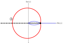
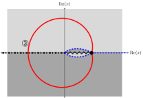
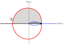
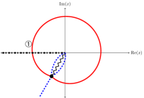
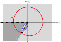
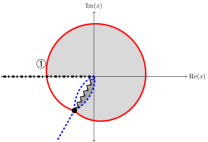
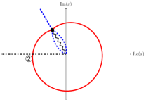
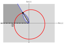
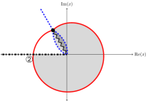
(a) Stokes structure of (41) in the $x$-plane. (b) Regions of validity of (41) in the $x$-plane. (c) Extended regions of validity of (41) in the $x$-plane. (d) Stokes structure of (42) in the $x$-plane. (e) Regions of validity of (42) in the $x$-plane. (f) Extended regions of validity of (42) in the $x$-plane. (g) Stokes structure of (43) in the $x$-plane. (h) Regions of validity of (43) in the $x$-plane. (i) Extended regions of validity of (43) in the $x$-plane.

Figure 3.6: This figure illustrates the Stokes structure of Type A solutions (41)-(43) of (5) in the complex $x$-plane with $q=1+0.2i$. Under the inverse transformation (44), the Stokes and anti-Stokes curves are now described by $q$-spirals in the $x$-plane. The branch cuts of the singulants, $\chi$, in the $x$-plane extend from the singularities and terminate at the origin. As we are using the leading order term of the inverse transformation in the limit $\epsilon\rightarrow 0$, the boundaries of $\mathcal{D}_{0}$ are mapped to the negative real $x$ axis, which corresponds to a logarithmic branch cut. Figure 6(b) illustrates the region of validity (light grey shaded regions) of (41) which contain a free parameter hidden beyond-all-orders. The regions of validity of (41) for which $\mathcal{S}^{-}_{3}$ is uniquely specified are illustrated in Figure 6(c). The corresponding Stokes structure and regions of validity for the remaining two Type A solutions are illustrated in Figures 6(d)-6(i).

The corresponding analysis of the Stokes structure and switching behaviour of the exponential contributions associated with the asymptotic solutions (42) and (43) may be obtained by using the symmetry (7). Consequently, the Stokes structure associated with $\chi_{1}$ and $\chi_{2}$ are vertical translations of the $\chi_{3}$-Stokes structure by $\mp 2i\pi$, respectively. The corresponding figures are contained in Figure 3.5.

As the Stokes structure and switching behaviour of the exponential contributions have been determined in the domain $\mathcal{D}_{0}$, we may finally determine the Stokes structure in the original complex $x$-plane. In order to determine the Stokes structure in the $x$-plane we reverse the scaling transformations. In particular, from the scalings given by (6) we find that the leading order mapping from $s$ to $x$ is given by

$$s=\frac{\epsilon\log(x)}{\log(1+\epsilon)}\sim\log(x)+\mathcal{O}(\epsilon),$$ (44)

as $\epsilon\rightarrow 0$.

We illustrate the Stokes structures of Type A solutions for the choice of $q=1+0.2i$. Using (44), the singulants, $\chi_{j}(s)$, can be written as a function of $x$. We then compute the Stokes structure in the complex $x$-plane using Matlab. The corresponding Stokes structure for the asymptotic solution described by (41) in the complex $x$-plane is illustrated in Figure 6(a). In these figures, the (anti-) Stokes curves and branch cuts in the complex $x$-plane follow the convention illustrated in Figure 3.1.

In particular, the complex $x$-plane contains a logarithmic branch cut (dot-dashed curve) along the negative real $x$ axis as a result of using the leading order term of the inverse transformation described by (44). In fact, the boundaries of $\mathcal{D}_{0}$ are mapped to this branch cut in the complex $x$-plane. The inverse transformation maps the Stokes and anti-Stokes curves in the $s$-plane to $q$-spirals in the complex $x$-plane. From Figure 3.6, we find the Stokes and anti-Stokes curve separate the complex $x$-plane into sectorial regions bounded by arcs of spirals.

4 Type B Asymptotics

In this section we investigate Type B solutions of (5). These are the asymptotic solutions of (5), which are described by $W_{0,4}$ to leading order as $\epsilon\rightarrow 0$. The analysis involved in the subsequent sections is nearly identical to Sections 2 and 3. Hence, we will omit the details and only provide the key results.

Type B solutions may be expanded as a power series in $\epsilon$ of the form

$$W(s)\sim W_{0,4}(s)+\sum_{r=1}^{\infty}\epsilon^{r}y_{r}(s),$$ (45)

as $\epsilon\rightarrow 0$. Following the analysis for Type A solutions, it can be shown that the behaviour of $y_{r}$ is also described by a factorial-over-power form. The behaviour of $y_{r}$ is therefore described by

$$y_{r}(s)\sim\frac{Y(s)\Gamma(r+\nu)}{\eta(s)^{r+\nu}},$$

as $r\rightarrow\infty$. Recall that the main difference between Type A and Type B solutions is that Type B solutions are singular at three distinct points in $\mathcal{D}_{0}$ rather than one. This feature will therefore be encoded in the calculation of the singulant function, $\eta$.

Since the leading order behaviour $W_{0,4}$ is singular at $s_{0,1},s_{0,2}$ and $s_{0,3}$, we obtain three singulant contributions, which we denote by $\eta_{j}(s)$. This feature can be deduced from equation (17), which shows that $W_{0,4}$ is expressible as the sum of $W_{0,1},W_{0,2}$ and $W_{0,3}$. Following the analysis in Section 3.1, $\eta_{j}(s)$ is given by

$$\eta_{j}(s)=\int_{s_{0,j}}^{s}\cosh^{-1}(\sigma(t))dt,$$ (46)

for $j=1,2,3$ and where $\sigma$ is given in (26) with $W_{0,3}$ replaced by $W_{0,4}$. Hence we obtain three contributions for $\eta$. Using the results for the late-order terms found in Section 3.1, we find that the late-order terms of (45) is given by

$$y_{r}(s)\sim\sum_{j=1}^{3}\frac{Y_{j}(s)\Gamma(r+\nu)}{\eta_{j}(s)^{r+\nu}},$$ (47)

as $r\rightarrow\infty$, and where $Y_{j}(s)$ are the prefactor terms associated with $\eta_{j}(s)$. Hence the asymptotic expansion of Type B solutions of (5) is given by

$$W(s)\sim W_{0,4}(s)+\sum_{j=1}^{3}\sum_{r=1}^{\infty}\frac{\epsilon^{r}Y_{j}(s)\Gamma(r+\nu)}{\eta_{j}(s)^{r+\nu}},$$ (48)

as $\epsilon\rightarrow 0$. As there are three distinct singulant terms in (48) there will be three subdominant exponentials present (after optimal truncation) and hence Type B solutions will also display Stokes behaviour.

By applying the Stokes smoothing technique demonstrated in Section 3.2 to (48), the expression which captures the Stokes behaviour of the subdominant exponential correction terms is given by

$$W(s)\sim W_{0,4}+\sum_{j=1}^{3}\sum_{r=1}^{2N_{\text{opt}}-1}\frac{\epsilon^{r}Y_{j}(s)\Gamma(r+\nu)}{\eta_{j}(s)^{r+\nu}}+\sum_{j=1}^{3}\mathcal{\hat{S}}_{j}(s)\hat{\phi}(s)Y_{j}(s)e^{-\eta_{j}(s/\epsilon)},$$ (49)

as $\epsilon\rightarrow 0$, and where $N_{\text{opt}}$ is the optimal truncation point. In particular, the Type B prefactor terms satisfy equation (32) with $W_{0}$ replaced by $W_{0,4}$. Similarly, the Stokes multipliers $\mathcal{\hat{S}}(s)$ satisfy (76) with $W_{0}$ and $\chi$ replaced by $W_{0,4}$ and $\eta$ respectively. In view of the formula (17), the leading order behaviour of the Type B solution is a composition of the leading order behaviours of Type A solutions. Consequently, the Stokes behaviour present in this solution will be more complicated as the Stokes curves emanate from more than one point as this allows the possibility of interaction effects. In order to determine the Stokes structure of Type B solutions, we analyze the singulant (46).

4.1 Stokes Structure

The Stokes structure of Type B asymptotic solutions in $\mathcal{D}_{0}$ is illustrated in Figure 4.1. In Figure 4.1 we see that there are three Stokes and two anti-Stokes curves curves emanating from each of the singularities, $s_{0,j}$, for $j=1,2,3$. The Stokes structure for Type B solutions is more complicated as there are Stokes curves which cross into the branch cuts (zig-zag curves) of $\eta_{j}$ as illustrated in Figure 4.1. As these Stokes curves continue onto another Riemann sheet of $\eta_{j}$, they may be subject to possible interaction effects from singularities originating in these Riemann sheets.

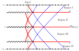
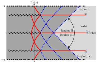
(a) Stokes structure of (49) in the complex $s$-plane. (b) Behaviour of $e^{-\eta_{j}/\epsilon}$ in the complex $s$-plane.

Figure 4.1: Stokes structure of the series solution (49) of (5) in the domain $\mathcal{D}_{0}$. Regions I-IV denote regions in which the exponential contributions associated with $\eta_{j}$, which is given by (46), are exponentially small and therefore denote the regions of validity for (49).

However, we observe from Figure 4.1 that there are regions which do not contain the Stokes curves continuing into the different Riemann sheets of $\eta_{j}$. These regions are labelled as regions I-IV in Figure 4.1. We first note that the Stokes curves emanating from the singularities $s_{0,1},s_{0,2}$ and $s_{0,3}$ asymptote to infinity as $\text{Re}(s)\rightarrow\infty$ as illustrated in Figure 1(a). In Figure 1(a), we find that region I is the region bounded by the upper boundary of $\mathcal{D}_{0}$, the upper anti-Stokes curve emanating from $s_{0,1}$ and the Stokes curve emanating from $s_{0,2}$, which is labelled by ➁; region II is the region bounded by the upper anti-Stokes curve emanating from $s_{0,1}$, and the Stokes curves labelled by ➁ and ➂; region III is the region bounded by the lower anti-Stokes curve emanating from $s_{0,2}$, and the Stokes curves labelled by ➀ and ➂; and finally region IV is the region bounded by the lower boundary of $\mathcal{D}_{0}$, the lower anti-Stokes curve emanating from $s_{0,2}$ and the Stokes curve emanating from $s_{0,1}$, which is labelled by ➀.

Furthermore, $\text{Re}(\eta_{j})$ is positive in each of these four regions and hence the exponential contributions associated with $\eta_{j}$ are exponentially small there. This is illustrated by the light grey shaded regions in Figure 1(b). We therefore restrict our analysis to regions I-IV as these are the regions in which the dominant asymptotic behaviour is described by (49). Consequently, the regions of validity of Type B solutions are the regions bounded by the upper and lower anti-Stokes curves emanating from the singularities, $s_{0,1}$ and $s_{0,2}$, respectively, and the boundaries of $\mathcal{D}_{0}$ containing the positive real $s$ axis. This is the union of regions I-IV and is illustrated in Figure 1(b).

In order to determine Stokes behaviour present in the asymptotic solution (49) we investigate the behaviour of $\eta_{j}$ in regions I-IV. In Figure 4.1, regions I-IV denotes those of $\mathcal{D}_{0}$ in which $\text{Re}(\eta_{j})>0$. Additionally, the imaginary parts of $\eta_{j}$ for $j=1,2,3$ are all positive in region I, whereas they are all negative in region IV. Furthermore, we have $\text{Im}(\eta_{1})>0$, $\text{Im}(\eta_{2})<0$, $\text{Im}(\eta_{3})>0$ in region II while $\text{Im}(\eta_{1})>0$, $\text{Im}(\eta_{2})<0$, $\text{Im}(\eta_{3})<0$ in region III.

Hence, the Stokes curve separating regions I and II switches on the exponential contribution associated with $\eta_{2}$, the Stokes curve separating regions II and III switches on the exponential contribution associated with $\eta_{3}$ and the Stokes curve separating regions III and IV switches on the exponential contribution associated with $\eta_{1}$. To denote the Stokes switching behaviour of these subdominant exponentials, the Stokes curves are labelled by ➀, ➁ and ➂.

In regions I-IV, the presence of the exponential contributions associated with $\eta_{j}$ are exponentially small since $\text{Re}(\eta_{j})>0$, and therefore do not affect the dominance of the leading order behaviour in (49). Hence, the values of $\mathcal{\hat{S}}_{j}$ may be freely specified in these regions and therefore the asymptotic solution described by (49) contains free parameters hidden beyond-all-orders.

In Section 3.3 we were able to obtain special asymptotic solutions by uniquely specifying the free parameters present in the asymptotic expansion. However, this cannot be done for Type B solutions in the same way because of the possible interaction effects of singularities originating from the different Riemann sheets of $\eta_{j}$.

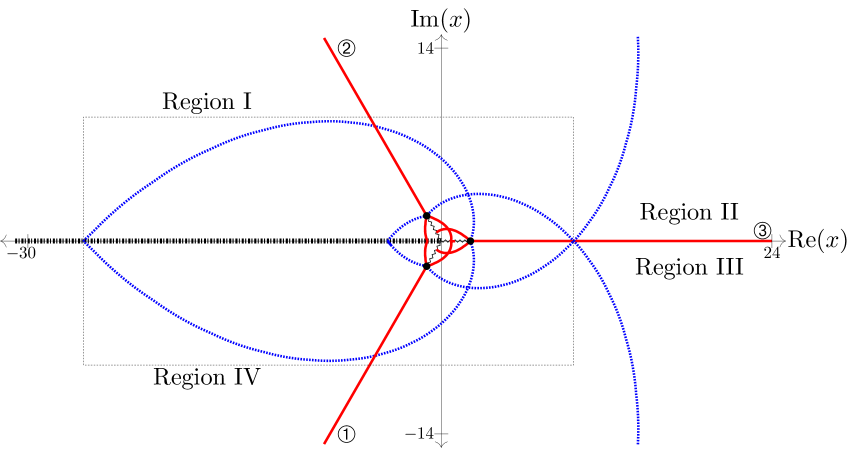
(c) Stokes structure associated with $\eta_{j}$ in the complex $x$-plane

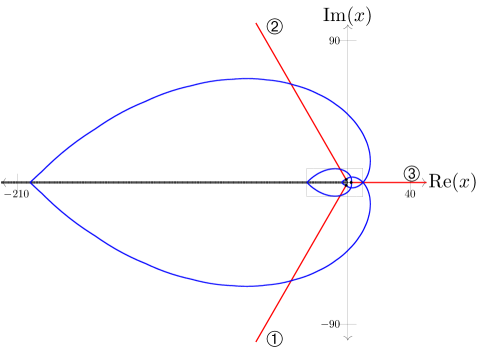
(d) Zoomed out version of Figure 4.2

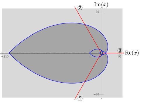
(e) Regions of validity

Figure 4.2: This figure illustrates the Stokes structure of type B solutions of $q$-$\text{P}_{\text{I}}$ in the original $x$-plane. Under the inverse transformation (44) the Stokes and anti-Stokes curves are described by $q$-spirals in the $x$-plane. The exponential contributions associated with $\eta_{1},\eta_{2}$ and $\eta_{3}$ are switched across the Stokes curves labelled by ➀, ➁ and ➂, respectively as illustrated in Figure 4.2. In Figure 4.2 the regions shaded in blue denote regions in which the asymptotic solution described by (49) is valid. These are the regions in which the exponential contributions present in (49) are exponentially small. The regions shaded in red are regions in which these exponential contributions are exponentially large and hence regions in which the asymptotic behaviour is not described by (49).

It may be possible to find special Type B solutions by considering the behaviour of the exponential contributions on the different Riemann sheets of $\eta_{j}$ and how they interact with those on the principal Riemann sheet. As this is beyond the scope of this study, we restrict our analysis to regions I-IV and therefore only obtain asymptotic solutions described by (49) which contain free parameters hidden beyond-all-orders.

Following the analysis in Section 3.3 we obtain the Stokes structure in the original $x$-plane by applying the inverse transformation given by (44). As in Section 3.3 we demonstrate the Stokes structure for the value of $q=1+0.2i$. Using Matlab, the Stokes structure of Type B solutions is illustrated in Figure 4.2.

Figure 4.2 shows the corresponding regions I-IV in the complex $x$-plane. In this figure, the Stokes and anti-Stokes curves are denoted by the solid red and dashed blue curves respectively. The branch cuts of $\eta_{j}$ are depicted as the zig-zag curves, which connect the singularities to the origin in the complex $x$-plane. Furthermore, the dot-dashed curve denotes the logarithmic branch cut defined by the reverse transformation (44) for the choice of $q=1+0.2i$.

Recall that the inverse transformation maps the Stokes and anti-Stokes curves in the complex $s$-plane to $q$-spirals in the complex $x$-plane. In particular, we see in Figure 4.2 that the Stokes curves of Type B solutions extend to infinity in the complex $x$-plane. This is due to the fact that the Stokes curves in the complex $s$-plane extend to infinity as $\text{Re}(s)\rightarrow\infty$ as shown in Figure 1(a). This was not case for the Stokes curves of Type A solutions in Section 3.3. Instead the Stokes curves of Type A solutions emanate from the singularities and approach the logarithmic branch cuts and enter a different Riemann sheet of the inverse transformation; this is illustrated in Figures 6(a), 6(d) and 6(g).

We have therefore determine the regions of validity for Type B solutions of $\text{$q$-P}_{\text{I}}$, (5), in the complex $x$-plane. Type B solutions are described by the asymptotic power series expansion (49) as $\epsilon\rightarrow 0$, and contain free parameters hidden beyond-all-orders. Furthermore, we have also calculated the Stokes behaviour present within these asymptotic solution, (49), which allowed us to determine regions in which this asymptotic description is valid.

5 Connection between Type A and Type B solutions and the nonzero and vanishing asymptotic solutions of $q$-Painlevé I

In this section we establish a connection between both Type A and B solutions found in this study to the nonzero and vanishing asymptotic solutions of $q$-Painlevé I respectively. We recall that the nonzero and vanishing asymptotic solutions were first found by Joshi in [28]. In particular, equation (1) admits solutions with the following behaviour

$$w(x)\sim w_{\rm{nv}}(x)=\omega^{3}+\mathcal{O}\left(\frac{1}{x}\right),\qquad w(x)\sim w_{\rm{v}}(x)=\frac{1}{x}+\mathcal{O}\left(\frac{1}{x^{4}}\right),$$ (50)

as $|x|\rightarrow\infty$, where $w_{\rm{nv}}$ and $w_{\rm{v}}$ are the nonzero and vanishing asymptotic solutions and $\omega^{3}=1$.

Recall that the four possible solutions for $W_{0}(s)$ are denoted by $W_{0,j}(s)$, which are defined by (15)-(16). In our investigation, we applied the scalings given in (4), in which the variable $x$ has the behaviour described by (6) as $\epsilon\rightarrow 0$. The analysis for both Type A and B solutions are valid in the limit $\epsilon\rightarrow 0$, which was shown to be equivalent to the double limit $|q|\rightarrow 1$ and $n\rightarrow\infty$. Under the additional limit, $s\rightarrow+\infty$, we see that the behaviour of $x$ in (6) approaches infinity. Therefore, the limits $\epsilon\rightarrow 0$ and $s\rightarrow+\infty$ are equivalent to the limit $|x|\rightarrow\infty$.

We now study the behaviour of $W_{0,j}(s)$ under the additional limit $s\rightarrow+\infty$. By applying the limit $s\rightarrow+\infty$ to the terms appearing in (13) and (14) we find from equations (15) and (16) that

$$\lim\limits_{s\rightarrow+\infty}W_{0,1}=-\frac{1}{2}+i\frac{\sqrt{3}}{2},\quad\lim\limits_{s\rightarrow+\infty}W_{0,2}=-\frac{1}{2}-i\frac{\sqrt{3}}{2},\quad\lim\limits_{s\rightarrow+\infty}W_{0,3}=1,\quad\lim\limits_{s\rightarrow+\infty}W_{0,4}=0.$$ (51)

The limiting behaviour of Type A solutions under the limit $s\rightarrow+\infty$ are therefore described by cube roots of unity. That is $W_{0,j}\sim\omega^{3},$ as $\epsilon\rightarrow 0$ and $s\rightarrow+\infty$ for $j=1,2,3$. However, we also find from (51) that Type B solutions vanish in the limit $s\rightarrow+\infty$. We therefore find that Type A solutions of (5) tend to the nonzero asymptotic behaviour solutions, $w_{\rm{nv}}$, found by Joshi [28] under the additional limit $s\rightarrow+\infty$.

In order to calculate the leading order behaviour of $W_{0,4}(s)$ as $s\rightarrow+\infty$, we need to keep terms up to order $\mathcal{O}(e^{-3s})$. Be carefully tracking such terms we find that the behaviour of Type B solutions are given by

$$W_{0,4}\sim\frac{1}{2}\sqrt{1-\frac{4e^{-s}}{3}}-\frac{1}{2}\sqrt{-\left(1-\frac{4e^{-s}}{3}\right)+\frac{2}{1-4e^{-s}/3}}\sim e^{-s}+\mathcal{O}(e^{-3s}),$$ (52)

as $s\rightarrow+\infty$. From (6) we find that (52) is equivalent to the behaviour $1/x$ as $|x|\rightarrow\infty$ and hence Type B solutions correspond to the vanishing asymptotic behaviour, $w_{\rm{v}}$, of (1).

5.1 Numerical computation for $q$-Painlevé I

In this section we give a numerical example of (3) with the parameter choice of $q=1+0.2i$ and where $x=x_{0}q^{n}$ with $x_{0}=1$. Given two initial conditions, $w_{0}$ and $w_{1}$, a sequence of solutions of (3) may be obtained by repeated iteration. In general, only a certain choice of initial conditions will give a solution of (3) which tends to the asymptotic behaviour of interest. We follow the numerical method demonstrated by [31], originally based on the works of [29] to find appropriate initial conditions which tend to Type A solutions of (3).

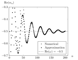
(a) Numerical values of $\text{Re}(w_{n})$.

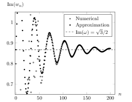
(b) Numerical values of $\text{Im}(w_{n})$

Figure 5.1: This figure illustrates the behaviour of the solutions to (3) with $q=1+0.2i$. The boundary conditions are chosen such that $w_{0}=0.846885522+i0.798385416$ and $w_{1}=-0.502881648-i0.650433326$. The values of $w_{n}$ are represented as blue circles, and the Type A asymptotic solution, $w_{n}\sim\omega$ as $n\rightarrow\infty$, where $\omega^{3}=1$, is represented by the black cross marks. From Figures 5.1 and 5.1 we see that the behaviour of the difference equation tends to the asymptotic expression for large $n$.

Figure 5.1 illustrates a comparison between the numerical solution of (3) with $q=1+0.2i$ and the initial conditions $w_{0}=0.846885522+i0.798385416$ and $w_{1}=-0.502881648-i0.650433326$ and the nonzero asymptotic solution, $w_{\text{nv}}$ in (50) with $\omega=(-1+i\sqrt{3})/2$. Figure 5.1 and 5.1 show that real and imaginary part of $w_{n}$ converges to $-1/2$ and $\sqrt{3}/2$ respectively for large $n$, which is precisely described by the leading order term of $w_{\text{nv}}$ in (50).

6 Conclusions

In this study, we extended the exponential asymptotic methods used in [31, 32] to compute and investigate Stokes behaviour present in the asymptotic solutions of $\text{$q$-P}_{\text{I}}$ in the double limit $\left|q\right|\rightarrow 1$ and $n\rightarrow\infty$. In order to investigate the solution behaviour of $q$-difference equations we rescaled the variables in the problem such that the double limit $\left|q\right|\rightarrow 1$ and $n\rightarrow\infty$ was equivalent to the limit $\epsilon\rightarrow 0$. We found two types of solutions for $\text{$q$-P}_{\text{I}}$, which we call Type A and Type B solutions. Type A solutions of $\text{$q$-P}_{\text{I}}$ are described asymptotically by either (41), (42) or (43), and Type B solutions are described by (49). The asymptotic descriptions obtained in this analysis are given as a sum of a truncated asymptotic power series and an exponentially subdominant correction term. We then determined the Stokes structure and used this information to deduce the regions of the complex plane in which these asymptotic solutions are valid.

In Section 3 we first considered the asymptotic solutions of (5) described by Type A solutions. Using exponential asymptotic methods, we determined the form of the subdominant exponential contribution present in the asymptotic solutions, which were found to be defined by one free Stokes switching parameter. From this behaviour, we deduced the associated Stokes structure, illustrated in Figures 1(a) and 3.5. By considering the Stokes switching behaviour of these subdominant exponentials, we found that the dominant asymptotic behaviour is described by either (41), (42) or (43) in a region in the complex $s$-plane containing the positive real axis. Furthermore, we found that it is possible to select the Stokes parameters so that the exponential contribution is absent in the regions where it would normally be large. Consequently, the regions of validity for the special Type A solutions are larger than the regions of validity for generic Type A solutions as illustrated in Figures 3(b), 5(b) and 5(d).

In Section 4, we considered the equivalent analysis for Type B solutions of (5). Compared to Type A solutions, Type B solutions are those which are singular at three points rather than one. Although exponential asymptotic methods may be used again to determine the form of the exponential small contributions present in Type B solutions, we noted that the analysis is near identical except for the determination of the singulant of this problem, $\eta$. The main difference is due to the fact that Type B solutions are singular at three points rather than one, and the remaining analysis was therefore identical as for Type A solutions. Type B asymptotic solutions are given as a sum of a truncated asymptotic power series and three exponentially subdominant correction terms as described in (49). The Stokes structure for Type B solutions, illustrated in Figure 4.1, is significantly more complicated than the Stokes structure of Type A solutions. In order to describe the Stokes switching behaviour in the domain $\mathcal{D}_{0}$ we must understand how the asymptotic solution (49) interacts with solutions on different Riemann sheets. However, we restrict ourselves to regions I-IV as these regions are free of possible interaction effects with singularities originating from the different Riemann sheets. Furthermore, all three exponential contributions present in Type B solutions are exponentially subdominant in regions I-IV and therefore represent the regions of validity of (49). Consequently, the asymptotic solutions described by (49) contain one free parameter defined by the Stokes multiplier.

By reversing the rescaling transformations we were then able to obtain the corresponding Stokes structure in the complex $x$-plane and found that the Stokes and anti-Stokes curves are described by $q$-spirals in the complex $x$-plane. As a result, the regions of validity are no longer described by traditional sectors bounded by rays but sectorial regions bounded by arcs of spirals. Consequently, this methodology is applicable to other $q$-Painlevé equations or more generally nonlinear $q$-difference equations in order to obtain asymptotic solutions which display Stokes phenomena.

Finally, Section 5 demonstrated that Type A and B solutions are related to the nonzero asymptotic and vanishing asymptotic solutions found by Joshi [28]. If the additional limit $s\rightarrow+\infty$ is also taken, then we find that Type A solutions correspond to the nonzero asymptotic solutions of $\text{$q$-P}_{\text{I}}$ while Type B solutions correspond to the quicksilver solutions of $\text{$q$-P}_{\text{I}}$ [28].

Appendix A Calculating the late-order terms near the singularity

In order to determine the value of $\gamma_{1}$ in (21) we calculate the local behaviour of $\chi_{3}$ and $U_{3}$. Using (20) in equations (26) and (32) we can show that

$$\chi_{3}(s)\sim\frac{4i\sqrt{6\sqrt{2}}}{5}(s-s_{0,3})^{5/4},\qquad U_{3}(s)\sim\frac{\Lambda}{\sqrt{i\sqrt{6\sqrt{2}}}(s-s_{0,3})^{1/8}},$$ (53)

as $s\rightarrow s_{0,3}$. Furthermore, by calculating the expression for $W_{1}$ (using equation (9)) it can be shown that $W_{1}(s)=\mathcal{O}\left((s-s_{0,3})^{-1/2}\right)$ and from (33) that

$$e^{\pm G(s)}=1\pm A_{1}(s-s_{0,3})^{1/4}+\mathcal{O}\left((s-s_{0,3})^{1/2}\right),$$ (54)

as $s\rightarrow s_{0,3}$ for some constant $A_{1}$. By substituting (53) into the expression for $W_{r}$ as given by (34) we find that the local behaviour of of the late-order terms near the singularity is given by

$$W_{r}(s)\sim \left(\frac{5}{4}\right)^{r+\gamma_{1}}\frac{\Gamma(r+\gamma_{1})}{\left(i\sqrt{6\sqrt{2}}\right)^{r+\gamma_{1}+1/2}(s-s_{0,3})^{5(r+\gamma_{1})/4+1/8}}\left(\Lambda e^{-G}+\frac{\tilde{\Lambda}e^{G}}{(-1)^{r+\gamma_{1}}}\right),$$ (55)

as $s\rightarrow s_{0,3}$. From (9), the dominant behaviour of $W_{r}$ is due to the term $W_{r-2}^{\prime\prime}/(4W_{0}^{3}-1)$. Hence, if $W_{r-2}$ has a singularity of strength $\nu$, then $W_{r}$ has one of strength $\nu+5/2$. In particular, since we know that $W_{0}$ is singular at $s_{0,3}$ of strength $-1/2$ then $W_{2r}$ will also be singular at $s_{0,3}$ but with strength $5r/2-1/2$. Moreover, since $W_{1}$ is also singular at $s_{0,3}$ of strength $1/2$, then $W_{2r+1}$ has one of strength $5r/2+1/2$.

We first observe from (54) that

$$\left(\Lambda e^{-G}+\frac{\tilde{\Lambda}e^{G}}{(-1)^{r+\gamma_{1}}}\right)\sim\begin{cases*}\Lambda+i\tilde{\Lambda}+A_{1}(-\Lambda+i\tilde{\Lambda})(s-s_{0,3})^{1/4}+\mathcal{O}((s-s_{0,3})^{1/2}),\quad\text{for even $r$,}\\ \Lambda-i\tilde{\Lambda}+A_{1}(-\Lambda-i\tilde{\Lambda})(s-s_{0,3})^{1/4}+\mathcal{O}((s-s_{0,3})^{1/2}),\quad\text{for odd $r$,}\end{cases*}$$ (56)

as $s\rightarrow s_{0,3}$. Thus, in order for the singularity behaviour of (55) to be consistent with that of $W_{2r}$, we require that $5r/2-1/2=5(2r+\gamma_{1})/4+1/8$ under the condition $\Lambda+i\tilde{\Lambda}\neq 0$. Hence, we deduce that $\gamma_{1}=-1/2$. Using the same argument, it can be shown that in order for $W_{2r+1}$ to have the correct singular behaviour in the limit $s\rightarrow s_{0,3}$ we must impose the condition $\Lambda-i\tilde{\Lambda}=0$, which gives

$$\tilde{\Lambda}=-i\Lambda.$$ (57)

Appendix B Calculating the prefactor constants via the inner problem

The expression for the late-order terms given by (21) contains a constant $\Lambda_{3}$, which is yet to be determined. In order to determine the value of $\Lambda_{3}$ we perform an inner analysis of (5) near the singularity, $s_{0,3}$ and determine the inner expansion of the inner solution. We then use the method of matched asymptotics to match the outer expansion to the inner expansion following Van Dyke’s matching principle [23].

In view of the leading order behaviour given by (20), we study the inner solution by applying the scalings

$$s=s_{0,3}+\epsilon^{4/5}\zeta,\qquad W(s)=a_{3}+\epsilon^{2/5}\psi_{1}(\zeta)+\epsilon^{3/5}\psi_{2}(\zeta),$$ (58)

where $\zeta$ is the inner variable, $\psi_{1}$ and $\psi_{2}$ are the first two terms of the inner solution, $\psi$. In particular, we recall that

$$s_{0,3}=\frac{1}{3}\log\left(\frac{256}{27}\right),\quad a_{3}=\left(\frac{1}{4}\right)^{1/3},\quad b_{3}=\left(\frac{1}{8\sqrt{2}}\right)^{1/3}.$$ (59)

Substituting (58) into (5) we obtain

$$(a_{3}^{4}-a_{3}+e^{-s_{0,3}})+\epsilon^{2/5}(4a_{3}^{3}-1)\psi_{1}+ \epsilon^{3/5}(4a_{3}^{3}-1)\psi_{2}+\epsilon^{4/5}(6a_{3}^{2}\psi_{1}^{2}-e^{-s_{0,3}}\zeta+a_{3}^{3}\psi_{1}^{\prime\prime})$$

$$+ \epsilon\left(\frac{s_{0,3}}{2}e^{-s_{0,3}}+12a_{3}^{2}\psi_{1}\psi_{2}+a_{3}^{3}\psi_{2}^{\prime\prime}\right)+\mathcal{O}(\epsilon^{6/5})=0,$$ (60)

as $\epsilon\rightarrow 0$, and where the prime denotes derivatives with respect to $\zeta$. Using the values of $a_{3},b_{3}$ and $s_{0,3}$ given in (59) we find that the coefficients of $\epsilon^{0},\epsilon^{2/5}$ and $\epsilon^{3/5}$ are identically zero. Therefore, the leading order equation of the inner solution is given by

$$\psi_{1}^{2}-b_{3}^{2}\zeta+\frac{a_{3}}{6}\frac{d^{2}\psi_{1}}{d\zeta^{2}}=0,$$ (61)

as $\epsilon\rightarrow 0$. From equation (60) we see that the term $\psi_{2}$ does not appear in the leading order equation in the limit $\epsilon\rightarrow\infty$. This reinforces the fact that the odd terms are indeed negligible in the limit $\epsilon\rightarrow 0$ as the term $\psi_{2}$ corresponds to the first odd coefficient term in the outer problem (far field expansion), (8).

To study the inner solution, we analyze (61) in the limit $\left|\zeta\right|\rightarrow\infty$. Using the method of dominant balance, equation (61) has a solution described by $\psi_{1}\sim b_{3}\sqrt{\zeta}$ as $\left|\zeta\right|\rightarrow\infty$. For algebraic convenience, we rescale the inner solution by setting

$$\psi_{1}(\zeta)\sim b_{3}\sqrt{\zeta}\sum_{r=0}^{\infty}\frac{E_{r}}{\zeta^{5r/2}},$$ (62)

with $E_{0}=1$. We then substitute (62) into (61) and match terms of $\mathcal{O}(\zeta)$ in the limit $\left|\zeta\right|\rightarrow\infty$. Doing this, we obtain the following nonlinear recurrence relation

$$E_{r}=-\frac{1}{2b_{3}^{2}}\left(\frac{a_{3}b_{3}}{24}(5r-4)(5r-6)E_{r-1}+b_{3}^{2}\sum_{k=1}^{r-1}E_{r-k}E_{k}\right),$$ (63)

for $r\geq 1$. We can express (62) in terms of the outer variables by reversing the scalings given in (58). Doing this, we find that the inner expansion of the outer solution is given by

$$W(s)\sim a_{3}+b_{3}\sum_{r=0}^{\infty}\frac{\epsilon^{2r}E_{r}}{(s-s_{0,3})^{(5r-1)/2}},$$ (64)

as $\epsilon\rightarrow 0$. Recall that the outer expansion is given by the expression (8) as $\epsilon\rightarrow 0$, and where the behaviour of coefficients are given by (35). By matching the expansions (8) and (64) it follows that

$$\Lambda_{3}=\lim\limits_{r\rightarrow\infty}b_{3}E_{r}\frac{\sqrt{i\sqrt{6\sqrt{2}}}}{\Gamma(2r-1/2)}\left(\frac{4i\sqrt{6\sqrt{2}}}{5}\right)^{2r-\tfrac{1}{2}}.$$ (65)

We then compute the first 1000 $E_{r}$ terms using the recurrence relation (63). Then, by using the formula (65) we find numerically that the approximate value of $\Lambda_{3}$ is

$$\Lambda_{3}\approx-0.04364,$$ (66)

to four significant figures. The approximate value for $\Lambda_{3}$ is shown in Figure B.1.

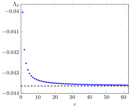
Figure B.1: This figure illustrates the approximation for $\Lambda$ appearing in the even late-order terms (55). As $r$ increases, the approximation for $\Lambda$ tends to the limiting value of $-0.04364$, which is denoted by the black dashed line.

Appendix C Stokes smoothing

To apply the exponential asymptotic method, we optimally-truncate the asymptotic series (8). One particular way to calculate the optimal truncation point is to consider where the terms in the asymptotic series is at its smallest [8]. This heuristic is equivalent to the finding $N$ such that

$$\bigg{|}\frac{\epsilon^{2N+2}W_{2N+2}}{\epsilon^{2N}W_{2N}}\bigg{|}\sim 1,$$

in the limit $N\rightarrow\infty$. By using the late-order form ansatz described by (21) we find that $N\sim|\chi_{3}|/(2\epsilon)$ as $\epsilon\rightarrow 0$ (which is equivalent to the limit $N\rightarrow\infty$). As this quantity may not necessarily be integer valued, we therefore choose $\kappa\in[0,1)$ such that

$$N_{\text{opt}}\sim\frac{1}{2}\left(\frac{\left|\chi_{3}\right|}{\epsilon}+\kappa\right),$$ (67)

is integer valued.

By substituting the truncated series, (36), into the governing equation (5) we obtain

$$\overline{T}T^{2}\underline{T}+T^{2}\underline{T}\overline{R}+2\overline{T}T\underline{T}R+\overline{T}T^{2}\underline{R}+\cdots=T+R-\frac{1}{(1+\epsilon)^{s/\epsilon}},$$ (68)

where the terms neglected are quadratic in $R_{N}$. We can use the recurrence relation (9) to cancel terms of size $o(\epsilon^{2N-1})$ in (68). In particular, equation (68) can be rewritten, after rearrangement, as

$$T^{2}\underline{T}\overline{R}+2\overline{T}T\underline{T}R+\overline{T}T^{2}\underline{R}-R\sim\epsilon^{2N}(4W_{0,3}^{3}-1)W_{2N},$$ (69)

as $\epsilon\rightarrow 0$ and where the terms neglected are of order $\mathcal{O}(\epsilon^{2N+1}W_{2N+1})$ and terms quadratic in $R_{N}$. Terms of these size are negligible compared to the terms kept in (69) as $\epsilon\rightarrow 0$.

Away from the Stokes curve the inhomogeneous terms of equation (69) are negligible as $\epsilon\rightarrow 0$. We may therefore apply a WKB analysis to the homogeneous version of (69) by setting $R_{N,\text{hom}}(s)=\alpha(s)e^{\beta(s)/\epsilon}$ as $\epsilon\rightarrow 0$. Using the WKB method, we find that the leading order equation gives the solution $\beta=-\chi_{3}$. Continuing to the next order involves matching terms of $\mathcal{O}(\epsilon R_{N})$. By collecting terms of this size in the homogeneous version of (69) we obtain the equation

$$-2W_{0,3}^{3}\sinh(\chi_{3}^{\prime})\frac{\alpha^{\prime}}{\alpha}-W_{0,3}^{3}\chi_{3}^{\prime\prime}\cosh(\chi_{3}^{\prime})+2W_{0,3}^{2}W_{0,3}^{\prime}\sinh(\chi_{3}^{\prime})+3\frac{W_{1}}{W_{0,3}}=0,$$ (70)

where we have substituted the fact that $\beta=-\chi_{3}$. Comparing equations (70) and (28) show that $\alpha$ satisfies to same differential equation as the prefactor $U_{3}$ and hence $\alpha\propto U_{3}$. Hence, away from the Stokes curves the solution of (69) is given by

$$R_{N,\text{hom}}(s)\sim U_{3}(s)e^{-\chi_{3}(s)/\epsilon},$$

as $\epsilon\rightarrow 0$.

In order to determine the Stokes switching behaviour associated with the optimally-truncated error, we set

$$R(s)=\mathcal{S}_{3}(s)R_{N,\text{hom}}(s),$$ (71)

where $\mathcal{S}_{3}(s)$ is the Stokes multiplier. We substitute (71) into (69) and use equations (25) and (28) to cancel terms. Doing this we find that the Stokes multiplier satisfies

$$\frac{d\mathcal{S}_{3}}{ds} \sim\frac{\epsilon^{2N-1}(1-4W_{0,3}^{3})W_{2N}}{2W_{0,3}^{3}\sinh(\chi_{3}^{\prime})\alpha(s)}e^{\chi_{3}/\epsilon}\sim\epsilon^{2N-1}\sqrt{1-4W_{0,3}^{3}}\frac{\Gamma(2N+\gamma_{1})}{\chi_{3}^{2N+\gamma_{1}}}e^{\chi_{3}/\epsilon},$$ (72)

as $\epsilon\rightarrow 0$.

Noting the form of $N$, we introduce polar coordinates by setting $\chi_{3}=\rho e^{i\theta}$ where the fast and slow variables are $\theta$ and $\rho$, respectively. This transformation tells us that

$$\frac{d}{ds}=-\frac{i\chi_{3}^{\prime}e^{-i\theta}}{\rho}\frac{d}{d\theta},$$ (73)

and (67) becomes $N_{\rm{opt}}=(\rho/\epsilon+\kappa)/2$. Under this change of variables equation (72) becomes

$$\frac{d\mathcal{S}_{3}}{d\theta}\sim\frac{i\sqrt{2\pi\rho}\sqrt{1-4W_{0,3}^{3}}}{\chi_{3}^{\prime}}\exp\left(\frac{\rho}{\epsilon}(e^{i\theta}-1-i\theta)-i\theta(\kappa-3/2)\right),$$ (74)

as $\epsilon\rightarrow 0$, where we have used Stirling’s approximation [1] of the Gamma function. For simplicity, we will let $H(s(\theta);\rho)=\sqrt{1-4W_{0,3}^{3}}/\chi_{3}^{\prime}$. From (74) we find that the right hand side is exponentially small everywhere except in the neighbourhood of $\theta=0$, which is exactly where the Stokes curve lies (where $\chi_{3}$ is purely real and positive). We now rescale about the neighbourhood of the Stokes curve in order to study the switching behaviour of $\mathcal{S}_{3}$ by setting $\theta=\sqrt{\epsilon}\hat{\theta}$. Note that under this scaling, $H(s(\theta);\rho)\sim H(|\chi_{3}|)$ as $\epsilon\rightarrow 0$, which is therefore independent of $\theta$ to leading order. Applying the scaling $\theta=\sqrt{\epsilon}\hat{\theta}$ to (74) gives

$$\frac{1}{\sqrt{\epsilon}}\frac{d\mathcal{S}_{3}}{d\hat{\theta}}\sim i\sqrt{2\pi\rho}H(|\chi_{3}|)\exp\bigg{(}-\frac{|\chi_{3}|\hat{\theta}^{2}}{2}\bigg{)},$$ (75)

as $\epsilon\rightarrow 0$. Integrating (75) we find that

$$\mathcal{S}_{3} \sim i\sqrt{2\pi\epsilon}H(\left|\chi_{3}\right|)\int^{\left|\chi_{3}\right|\hat{\theta}}e^{-x^{2}/2}dx=i\pi\sqrt{\epsilon}H(\left|\chi_{3}\right|)\left(\text{erf}\left(\theta\sqrt{\frac{\left|\chi_{3}\right|}{2\epsilon}}\right)+C_{3}\right),$$ (76)

where $C_{3}$ is an arbitrary constant. Thus, as Stokes curves are crossed, the Stokes multiplier changes in value by

$$\Delta\mathcal{S}_{3}\sim 2i\pi\sqrt{\epsilon}H(\left|\chi_{3}\right|),$$

and therefore

$$\Delta R_{N}\sim 2i\pi\sqrt{\epsilon}H(\left|\chi_{3}\right|)U_{3}(s)e^{-\chi_{3}(s)/\epsilon},$$

as $\epsilon\rightarrow 0$.

References

- [1] M. Abramowitz and I. A. Stegun. Handbook of Mathematical Functions with Formulas, Graphs, and Mathematical Tables. Dover Publications, Inc., New York, 1992.
- [2] C. M. Bender and S. A. Orszag. Advanced Mathematical Methods for Scientists and Engineers.I. Springer-Verlag, New York, 1999.
- [3] M. V. Berry. Stokes’ phenomenon; smoothing a Victorian discontinuity. Publ. Math. Inst. Hautes Études Sci., 68:211–221, 1988.
- [4] M. V. Berry. Uniform asymptotic smoothing of Stokes’ discontinuities. Proc. R. Soc. A, 422:7–21, 1989.
- [5] M. V. Berry. Asymptotics, superasymptotics, hyperasymptotics. In H. Segur, S. Tanveer, and H. Levine, editors, Asymptotics Beyond All Orders. Plenum, New York, 1991.
- [6] M. V. Berry and C. J. Howls. Hyperasymptotics. Proc. R. Soc. A, 430:653–668, 1990.
- [7] P. Boutroux. Recherches sur les transcendantes de m. Painlevé et l’étude asymptotique des équations différentielles du second ordre. Ann. Sci. École Norm. Sup., 30:255–375, 1913.
- [8] J. P. Boyd. The devil’s invention: asymptotic, superasymptotic and hyperasymptotic series. Acta Appl. Math., 56:1–98, 1999.
- [9] B. L. J. Braaksma, G. K. Immink, M. Van der Put, and J. Top, editors. Differential equations and the Stokes phenomenon. Proceedings of the workshop held at the University of Groningen, Groningen, May 28–30, 2001, World Scientific Publishing Co., Inc., River Edge, NJ, 2002.
- [10] É. Brézin and V. A. Kazakov. Exactly solvable field theories of closed strings. Phys. Lett. B, 236:144–150, 1990.
- [11] G. A. Cassatella-Contra and M. Mañas. Riemann-Hilbert problems, matrix orthogonal polynomials and discrete matrix equations with singularity confinement. Stud. Appl. Math., 128:252–274, 2012.
- [12] S. J. Chapman, C. J. Howls, J. R. King, and A. B. Olde Daalhuis. Why is a shock not a caustic? The higher-order Stokes phenomenon and smoothed shock formation. Nonlinearity, 20:2425–2452, 2007.
- [13] S. J. Chapman, J. R. King, and K. L. Adams. Exponential asymptotics and Stokes lines in nonlinear ordinary differential equations. Proc. R. Soc. A, 454:2733–2755, 1998.
- [14] S. J. Chapman and D. B. Mortimer. Exponential asymptotics and Stokes lines in a partial differential equation. Proc. R. Soc. A, 461:2385–2421, 2005.
- [15] P. A. Clarkson. Painlevé equations—nonlinear special functions. In Proceedings of the Sixth International Symposium on Orthogonal Polynomials, Special Functions and their Applications (Rome, 2001), volume 153, pages 127–140, 2003.
- [16] P. A. Clarkson, A. F. Loureiro, and W. Van Assche. Unique positive solution for an alternative discrete Painlevé I equation. J. Difference Equ. Appl., 22:656–675, 2016.
- [17] P. A. Deift and X. Zhou. A steepest descent method for oscillatory Riemann-Hilbert problems. Bull. Amer. Math. Soc. (N.S.), 26:119–123, 1992.
- [18] L. Di Vizio and C. Zhang. On -summation and confluence. Ann. Inst. Fourier (Grenoble), 59:347–392, 2009.
- [19] R. B. Dingle. Asymptotic Expansions: their Derivation and Interpretation. Academic Press, London-New York, 1973.
- [20] A. S. Fokas, A. R. Its, and A. V. Kitaev. Discrete Painlevé equations and their appearance in quantum gravity. Comm. Math. Phys., 142:313–344, 1991.
- [21] A. S. Fokas, A. R. Its, and A. V. Kitaev. The isomonodromy approach to matrix models in D quantum gravity. Comm. Math. Phys., 147:395–430, 1992.
- [22] P. J. Forrester and N. S. Witte. Painlevé II in random matrix theory and related fields. Constr. Approx., 41:589–613, 2015.
- [23] E. J. Hinch. Perturbation Methods. Cambridge University Press, Cambridge, 1991.
- [24] C. J. Howls and A. B. Olde Daalhuis. Exponentially accurate solution tracking for nonlinear ODEs, the higher order Stokes phenomenon and double transseries resummation. Nonlinearity, 25:1559–1584, 2012.
- [25] G. K. Immink. Resurgent functions and connection matrices for a linear homogeneous system of difference equations. Funkcial. Ekvac., 31:197–219, 1988.
- [26] A. R. Its. The Painlevé transcendents as nonlinear special functions. In D. Levi and P. Winternitz, editors, Painlevé Transcendents. Plenum, New York, 1992.
- [27] N. Joshi. A local asymptotic analysis of the discrete first Painlevé equation as the discrete independent variable approaches infinity. Methods Appl. Anal., 4:124–133, 1997.
- [28] N. Joshi. Quicksilver solutions of a -difference first Painlevé equation. Stud. Appl. Math., 134:233–251, 2015.
- [29] N. Joshi and A. V. Kitaev. On Boutroux’s tritronquée solutions of the first Painlevé equation. Stud. Appl. Math., 107:253–291, 2001.
- [30] N. Joshi and S. B. Lobb. Singular dynamics of a -difference Painlevé equation in its initial value space. J. Phys. A, 49:1–24, 2016.
- [31] N. Joshi and C. J. Lustri. Stokes phenomena in discrete Painlevé I. Proc. R. Soc. A, 471:1–22, 2015.
- [32] N. Joshi, C. J. Lustri, and S. Luu. Stokes phenomena in discrete Painlevé II. Proc. R. Soc. A, 473:1–20, 2017.
- [33] N. Joshi and P. Roffelson. Analytic solutions of - near its critical points. Nonlinearity, 29:3696–3742, 2016.
- [34] N. Joshi and Y. Takei. On Stokes phenomena for the alternate discrete PI equation. In Galina Filipuk, Yoshishige Haraoka, and Sławomir Michalik, editors, Analytic, Algebraic and Geometric Aspects of Differential Equations, pages 369–381. Birkhäuser/Springer, Cham, 2017.
- [35] J. R. King and S. J. Chapman. Asymptotics beyond all orders and Stokes lines in nonlinear differential-difference equations. European J. Appl. Math., 4:433–463, 2001.
- [36] A. Knizel. Moduli spaces of -connections and gap probabilities. Int. Math. Res. Not. IMRN, pages 6921–6954, 2016.
- [37] I. M. Krichever. Analytic theory of difference equations with rational and elliptic coefficients and the Riemann-Hilbert problem. Uspekhi Mat. Nauk, 59:111–150, 2004.
- [38] E. Laguerre. Sur la réduction en fractions continues d’une fraction qui satisfait à une équation différentielle linéaire du premier ordre dont les coefficients sont rationnels. J. Math. Pures Appl., 1:135–165, 1885.
- [39] A. P. Magnus. Painlevé-type differential equations for the recurrence coefficients of semi-classical orthogonal polynomials. J. Comput. Appl. Math., 57:215–237, 1995.
- [40] A. P. Magnus. Freud’s equations for orthogonal polynomials as discrete Painlevé equations. In Symmetries and Integrability of Difference Equations. Cambridge Univ. Press, 1999.
- [41] T. Mano. Asymptotic behaviour around a boundary point of the -Painlevé VI equation and its connection problem. Nonlinearity, 23:1585–1608, 2010.
- [42] T. Morita. A connection formula between the Ramanujan function and the -Airy function. arXiv preprint arXiv:1104.0755v2, 2011.
- [43] T. Morita. The Stokes phenomenon for the -difference equation satisfied by the basic hypergeometric series . In Novel Development of Nonlinear Discrete Integrable Systems. Res. Inst. Math. Sci. (RIMS), Kyoto, 2014.
- [44] T. Morita. The Stokes phenomenon for the Ramanujan’s -difference equation and its higher order extension. arXiv preprint arXiv:1404.2541v1, 2014.
- [45] S. Nishioka. Transcendence of solutions of -Painlevé eqution of type . Aequationes Math., 79:1–12, 2010.
- [46] Y. Ohyama. -Stokes phenomenon of a basic hypergeometric series . J. Math. Tokushima Univ., 50:49–60, 2016.
- [47] A. B. Olde Daalhuis. Inverse factorial-series solutions of difference equations. Proc. Edinb. Math. Soc., 47:421–448, 2004.
- [48] A. B. Olde Daalhuis, S. J. Chapman, and J. R. King. Stokes phenomenon and matched asymptotic expansions. SIAM J. Appl. Math., 55:1469–1483, 1995.
- [49] F. W. J. Olver. Resurgence in difference equations, with an application to Legendre functions. In C. Dunkl, M. Ismail, and R. Wong, editors, Special Functions. World Scientific, 2000.
- [50] R. B. Paris. Smoothing of the Stokes phenomenon for high-order differential equations. Proc. R. Soc. A, 436:165–186, 1992.
- [51] V. Periwal and D. Shevitz. Exactly solvable unitary matrix models: Multicritical potentials and correlations. Nuclear Phys. B, 344:731–746, 1990.
- [52] V. Periwal and D. Shevitz. Unitary-matrix models as exactly solvable string theories. Phys. Rev. Lett., 64:1326, 1990.
- [53] J. P. Ramis, J. Sauloy, and C. Zhang. Local analytic classification of -difference equations. Astérisque, 355:vi+151, 2013.
- [54] S. Shimomura. Continuous limit of the difference second Painlevé equation and its asymptotic solutions. J. Math. Soc. Japan, 64:733–781, 2012.
- [55] J. Shohat. A differential equation for orthogonal polynomials. Duke Math. J., 5:401–417, 1939.
- [56] W. Van Assche. Discrete Painlevé equations for recurrence coefficients of orthogonal polynomials. In Difference equations, Special functions and Orthogonal polynomials, pages 687–725. World Sci. Publ., Hackensack, NJ, 2007.
- [57] W. Van Assche, G. Filipuk, and L. Zhang. Mutiple orthogonal polynomials associated with an exponential cubic weight. J. Approx. Theory, 190:1–25, 2015.
- [58] V. L. Vereshchagin. Asymptotic classification of solutions to the first discrete Painlevé equation. Sib. Math. J., 37:876–892, 1995.
- [59] V. L. Vereshchagin. Asymptotics of solutions of the discrete string equation. Phys. D, 95:268–282, 1996.
- [60] S. X. Xu and Y. Q. Zhao. Asymptotics of discrete Painlevé V transcendents via the Riemann-Hilbert approach. Stud. Appl. Math., 130:201–231, 2013.
- [61] C. Zhang. Sur la sommabilité des séries entières solutions formelles d’une équation aux -différences. I. Comptes Rendus de l’Académie des Sciences. Série I. Mathématique, 327:349–352, 1998.
- [62] C. Zhang. Une sommation discrète pour des équations aux -différences linéaires et à coefficients analytiques: théorie générale et exemples. In Differential Equations and the Stokes Phenomenon. World Sci. Publ., River Edge, NJ, 2002.
- [63] C. Zhang. Solutions asymptotiques et méromorphes d’équations aux -différences. Sémin. Congr., 14:341–356, 2006.