Heat kernel for Liouville Brownian motion and Liouville graph distance

Abstract

We show the existence of the scaling exponent $\chi\in(0,4[(1+\gamma^{2}/4)-\sqrt{1+\gamma^{4}/16}]/\gamma^{2}]$ of the graph distance associated with subcritical two-dimensional Liouville quantum gravity of paramater $\gamma<2$ on $\mathbb{V}=[0,1]^{2}$. We also show that the Liouville heat kernel satisfies, for any fixed $u,v\in\mathbb{V}^{o}$, the short time estimates

$$\lim_{t\to 0}\frac{\log|\log\mathsf{p}_{t}^{\gamma}(u,v)|}{|\log t|}=\frac{\chi}{2-\chi},\ \mbox{\rm a.s.}$$

1 Introduction

Let $\mathbb{V}=[0,1]^{2}\subseteq\mathbb{R}^{2}$ and let ${\mathbb{V}}^{o}$ denote its interior. Let $h$ be an instance of the Gaussian free field (GFF) on $\mathbb{V}$ with Dirichlet boundary condition. For an introduction to the theory of the GFF including various formal constructions, see, e.g., [36, 5]. Fix $\gamma\in(0,2)$ and let $M_{\gamma}$ denote the $\gamma$ Liouville quantum gravity (LQG) given by formally exponentiating the GFF $h$ [17]. One can then introduce the positive continuous additive functional (PCAF) with respect to $M_{\gamma}$ as

$$F(t):=\int_{0}^{t}e^{\gamma h(X_{s})-\frac{\gamma^{2}}{2}{\mathbb{E}}h(X_{s})^{2}}ds,$$ (1)

where $\{X_{t}\}$ denotes a standard Brownian motion (SBM) on $\mathbb{V}$ killed upon exiting $\mathbb{V}$, independent of $h$. The Liouville Brownian motion (LBM) is then defined formally as $Y_{t}:=X_{F^{-1}(t)}$, and the Liouville heat kernel (LHK) $\mathsf{p}_{t}^{\gamma}(x,y)$ is the density of the Liouville semigroup with respect to $M_{\gamma}$, i.e.

$$E^{x}f(Y_{t})=\int\mathsf{p}_{t}^{\gamma}(x,y)f(y)M_{\gamma}(dy),$$ (2)

where the superscript $x$ is to recall that $Y_{0}=X_{0}=x$. We refer to Section 2 for pointers to the (non-trivial) precise construction and properties of these objects.

For $\delta>0$ and any two distinct points $u,v\in{\mathbb{V}}^{o}$, we define the Liouville graph distance $D_{\gamma,\delta}(u,v)$ to be the minimal number of Euclidean balls with rational centers and LQG measure at most $\delta^{2}$, whose union contains a path from $u$ to $v$.

Theorem 1.1.

Fix $\gamma\in(0,2)$. There exists $\chi=\chi(\gamma)\in\big{(}0,\frac{4[(1+\gamma^{2}/4)-\sqrt{1+\gamma^{4}/16}]}{\gamma^{2}}\big{]}$ such that the following holds. For any $\iota>0$ and any fixed points $u\neq v\in{\mathbb{V}}^{o}$, there exists a random variable $C=C(\iota,u,v)$ measurable with respect to $h$ such that for all $\delta,t\in(0,1]$,

$$C^{-1}\delta^{-\chi+\iota} \leq D_{\gamma,\delta}(u,v)\leq C\delta^{-\chi-\iota}\,,$$ (3)

$$C^{-1}\exp\Big{\{}-t^{-\frac{\chi}{2-\chi}-\iota}\Big{\}} \leq\mathsf{p}_{t}^{\gamma}(u,v)\leq C\exp\Big{\{}-t^{-\frac{\chi}{2-\chi}+\iota}\Big{\}}\,.$$ (4)

As we now discuss, Theorem 1.1 is an amalgamation of several results, proved in different sections of the paper.

• The Liouville graph distance exponent $\chi$ is well defined (see Proposition 5.1) and the (log of the) distance concentrates around its mean (see Proposition 3.17).

• The distance exponent $\chi$ does not depend on the particular choice of $u$ and $v$ as long as they are fixed and away from the boundary (see Proposition 5.1).

• Both lower bounds and upper bounds on the Liouville heat kernel can be obtained from the distance exponent (see (80) and (106)): such bounds are sharp in terms of the power on $t$ in the exponential as in (4).

• The lower bound that $\chi>0$ is a relatively obvious result (see Lemma 2.12); the upper bound on $\chi$ is a reading from the KPZ relation established in [17], which is applied to bound the minimal number of Euclidean balls of LQG measure at most $\delta^{2}$ required in order to cover the line segment joining $u$ and $v$. Evaluating $\chi$ is a major open problem and is not the focus of the present article. We record the bounds here only to show that $\chi$ is nontrivial (i.e., $0<\chi<1$), and therefore the heat kernel in (4) is not diffusive.

• For $\gamma$ small, non-trivial upper bounds on $\chi$ appear in [13]. In particular, combining Theorem 1.1, [13, Theorem 1.2] and [25], one obtains that there exist constants $c^{*},c^{\prime}>0$ so that $\chi\in(1-c^{\prime}\gamma,1-c^{*}\gamma^{4/3}/|\log\gamma|)$ for small $\gamma$. In particular, as discussed in [13], this is incompatible with Watabiki’s conjecture. For some work toward bounding exponents for a related distance, see [21].

• It is a consequence of [16] and [13] that the Liouville graph distance is not universal across different log-correlated fields. Because of Theorem 1.1 and [14], the same holds for the Liouville heat kernel exponent.

1.1 Background and related results

Making a rigorous sense of the metric associated with the LQG is a well known major open problem, see [33] for an up-to-date review. In a recent series of works of Miller and Sheffield, the special case $\gamma=\sqrt{8/3}$ is treated; one of their achievements is to produce candidate scaling limits and to establish a deep connection to the Brownian map, see [26, 29, 27, 28] and references therein. In a recent work [21], upper and lower bounds have been obtained for a distance associated with the LQG (which is presumably related to Liouville graph distance considered in the present article), and for that distance the existence of the scaling exponent was established.

From another perspective, the LBM has also drawn much interest recently, after it was constructed in [20, 3]. In particular, the LBM heat kernel was constructed in [19], and on-diagonal bounds were derived in [32], implying that the spectral dimension of LBM equals $2$. Estimates on the off-diagonal behavior are more challenging, and some (weak, but non-trivial) bounds were established in [25] and [2], with a significant gap in the exponent between the upper and lower bounds. Building on [15], we have computed in [14] the exponent for the Liouville heat kernel on a so-called coarse modified branching random walk, and showed that the exponent is not universal among log-correlated Gaussian fields. The present article focuses on the GFF set-up and establishes that in the precision of the exponent, the off-diagonal LHK is closely related to the Liouville graph distance.

Another distance that has been considered in the literature is the Liouville first passage percolation (FPP), whose discrete version is the shortest distance metric where each vertex is given a weight of the exponential of the GFF value there. In [12], it was shown that at high temperatures the appropriately normalized Liouville FPP converges subsequentially in the Gromov-Hausdorff sense to a random distance on the unit square, where all the (conjecturally unique) limiting metrics are homeomorphic to the Euclidean distance. In [16], it was shown that the dimension of the geodesic for Liouville FPP is strictly larger than 1.

Finally, we mention two random walk models on the environment generated by GFF: in [9] a discrete analog of LBM was considered, where the holding times for the random walk at each vertex are exponential distributions with means given by the exponentials of the GFF — some scaling limit results were obtained for this model; in [7] a random walk on the random network generated by discrete GFF was considered, where in the random network each edge $(u,v)$ is assigned a resistance exponential in the sum of the GFF values at $u$ and $v$ — the return probability for this random walk was computed via a computation of the effective resistance of this random network.

1.2 A word on proof strategy and organization of the paper

Before describing our proof strategy, we discuss some of the basic objects that we work with. The first object is the Gaussian free field. There are many approaches for its construction, which we quickly review in Section 2.2. Of importance to us is its construction in terms of integral over space-time white noise, where the ‘time’ coordinate denotes scale. This allows naturally the split of the GFF into an independent sum of a ‘coarse’ field, consisting of contributions down to a cutoff scale, and a ‘fine’ field, consisting of the rest.

Next, the Gaussian multiplicative chaos built from the Gaussian free field, which we refer to as the Liouville quantum gravity, can be constructed as a martingale limit of the exponential of the coarse field associated with the GFF, see e.g. (27). In particular, it can be described as a product of a function depending only on the coarse field of the GFF, by an independent measure determined by the fine field; this yields a natural separation of scales, which however as we explain below is not quite sufficient for our analysis. For this reason, we often work with appropriate approximations of the LQG, see for example (13). In this sketch, we only mention such details when they are crucial to the argument.

We can now begin to discuss our proof strategies, starting with the Liouville graph distance. As is often the case, the proof of a scaling statement as in (3) is based on sub-additivity, which in this case will be with respect to the scale parameter. However, the Liouville graph distance from the introduction is not convenient to work with, because of the lack of scale-separation properties that are crucial for sub-additivity. Therefore, our first step is to relate the Liouville graph distance to an approximate Liouville graph distance, obtained through a specific partitioning procedure of the square according to the LQG content of dyadic squares, see Section 3.1 for details of the construction. Since the approximation involves a sequence of refinements, sub-additivity for the approximate Liouville graph distance is almost built in. However, we need to show that the approximate distance is indeed a good proxy for the distance. This is done in Proposition 3.2. Most of Section 3 is devoted to its proof, which employs appropriate approximations of the LQG and a-priori estimates of fluctuations of the coarse field of the GFF. A particularly annoying fact is that the coarse field fluctuations, which typically are well behaved, cannot be well controlled uniformly, and at places one needs to replace the actual minimizing sequence by a proxy, bypassing some bad regions of large fluctuations. This is done in Lemmas 3.12 and 3.13, which employ percolation arguments.

The approximate graph distance thus constructed also has better continuity properties in terms of the underlying GFF, and is instrumental in proving that the (logarithm of the) graph distance concentrates around its mean, see Proposition 3.17.

Once these preliminary tasks are complete, we turn in Section 4 to the study of off-diagonal short time Liouville heat kernel estimates. (We study the LHK before showing the convergence of the distance exponent in order to emphasize that the study of the LHK is independent of the latter.) Recall that the Liouville Brownian motion is constructed from simple Brownian motion by a time change that depends on the Liouville quantum gravity. In Section 4.1, we prove a lower bound on the LHK, by a technique introduced in [14]. We construct boxes according to the partition yielding the approximate Liouville graph distance. (In reality, we construct smaller sub-boxes in order to handle differing sizes of blocks in the partition, and bypass some bad regions in the geodesic, using Lemmas 3.12 and 3.13). In order to control the behavior of the LBM, we introduce the notion of ‘fast boxes’, which are boxes in which, from many starting points, the LBM does not accumulate more time change than typical. Boxes are fast with high probability, and using a Peierls argument, we show that they percolate; the lower bound on the LHK is obtained by forcing the LBM to follow such a path. For the upper bound, we introduce a parallel notion of ‘slow boxes’, which are cells in which, for enough starting points, the LBM typically accumulates at least a small fraction of the typical time-change. Most cells in the partition determining the approximate Liouville graph distance are slow, and by tracking the accumulated time change, we obtain a lower bound on the total accumulated time-change, which translates to a LHK upper bound. We emphasize that the upper bound is obtained in terms of a liminf of the Liouville graph distance exponent, while the lower bound is obtained in terms of a limsup.

Finally, in Section 5, we return to the Liouville graph distance. Using concentration inequalities, it is enough to prove convergence for the rescaled expectation of (the logarithm of) the approximate Liouville graph distance. Separation of scales is built into the definition, however translation invariance is not (due to boundary effects). Further, even though the approximate Liouville graph distance uses refinements in its construction and thus separation of scales, it still suffers from lack of independence across scales. These two factors prevent the direct use of sub-additivity. To obtain the latter, we introduce yet another version of the Liouville graph distance, which does possess the required invariance property and, while at a given scale, does not depend on the fine field in slightly smaller scales. A coupling argument allows us to couple the two distances, and sub-additivity can then be employed to give a point-to-point convergence of the rescaled log-distance (see Lemma 5.3), for points near the center of the box. This is already enough to give an upper bound for arbitrary points. To give a lower bound, it is not enough to control point-to-point distances, and we need to control point to boundary distances for small enough sub-boxes. The latter estimate involves the point-to-point estimate and a percolation argument, see Lemma 5.4.

Various preliminaries are collected for the convenience of the reader in Section 2. We also include, in Section 2.5, a derivation of rough estimates on the distance exponent. These estimates are not expected to be sharp.

1.3 Notation convention

We say that the events $E=E_{\delta}$ occur with high probability (with respect to $\delta$) if there exists a constant $c>0$, depending on $\gamma,\{E_{\delta}\}$ only, so that ${\mathbb{P}}(E_{\delta})\geq 1-\delta^{c}$ for all small $\delta>0$. For $\alpha>0$, we say that the events $E=E_{\delta}$ occur with $\alpha$-high probability, if ${\mathbb{P}}(E_{\delta})\geq 1-\delta^{\alpha}$ for all small $\delta>0$.

For (nonnegative) functions $F(\cdot)$ and $G(\cdot)$ we write $F=O(G)$ (alternatively, $\Omega(G)$) if there exists an absolute constant $C>0$ such that $F\leq CG$ (respectively $\geq CG$) everywhere in their domain. We write $F=\Theta(G)$ if $F$ is both $O(G)$ and $\Omega(G)$. If the constant depends on variables $x_{1},x_{2},\ldots,x_{n}$, we change these notations to $O_{x_{1},x_{2},\ldots,x_{n}}(G)$ and $\Omega_{x_{1},x_{2},\ldots,x_{n}}(G)$ respectively. We denote by $C,c,C^{\prime},c_{i}$ etc positive universal constants. For parameters or variables $p_{i}$, we write $C=C(p_{1},\ldots,p_{k})$ if $C$ is a positive constant that depends only on $p_{1},\ldots,p_{k}$. For example, $C(\gamma)$ is a positive constant that may depend on $\gamma$.

For $v\in\mathbb{R}^{2}$ and $r>0$, we denote by $B_{r}(v)$ the (open) Euclidean ball centered at $v$ of radius $r$. For $i\geq 1$ we denote by $\mathfrak{C}_{i}$ the collection of centers for all dyadic squares of side length $2^{-i}$ contained in $\mathbb{V}$. That is, with $o_{\mathrm{LB}}=(0,0)$,

$$\mathfrak{C}_{i}=\{o_{\mathrm{LB}}+(2^{-i-1},2^{-i-1})+(j\cdot 2^{-i},k\cdot 2^{-i}):0\leq j,k\leq 2^{i}-1\}.$$ (5)

Note that $|\mathfrak{C}_{i}|=2^{2i}$.

A box $B$ is a square in $\mathbb{R}^{2}$. We denote by $s_{B}$ the side of $B$ and by $c_{B}$ its center. We say that a box $B$ is a dyadic box if, for some $i\in\mathbb{N}$, $s_{B}=2^{-i}$ and $c_{B}\in\mathfrak{C}_{i}$. We say that a Euclidean ball $B$ is a dyadic ball if, for some $i\in\mathbb{N}$, the radius of $B$ is $2^{-i}$ and the center of $B$ is in $\mathfrak{C}_{i}$. Finally, we use $|\cdot|$ to denote the Euclidean distance and $|\cdot|_{\infty}$ to denote the $\ell_{\infty}$ norm.

2 Preliminaries

2.1 General Gaussian inequalities

The next lemma is a consequence of the the Borell–Sudakov-Tsirelson Gaussian isoperimetric inequality ([8, 37]).

Lemma 2.1.

For any constant $c>0$ there exists $C>0$ such that the following holds. Let $\mathbf{X}=(X_{1},\ldots,X_{n})$ be a centered Gaussian process with $\max_{1\leq i\leq n}{\rm Var}X_{i}=\sigma^{2}$. Let $B\subseteq\mathbb{R}^{n}$ such that ${\mathbb{P}}(\mathbf{X}\in B)\geq c$. Then for $\lambda\geq C\sigma$,

$${\mathbb{P}}(\min_{\mathbf{x}\in B}|\mathbf{X}-\mathbf{x}|_{\infty}\geq\lambda)\leq Ce^{-\frac{(\lambda-C\sigma)^{2}}{2\sigma^{2}}}\,.$$

Proof.

Let $\mathbf{X}=A\mathbf{Z}$ where $\mathbf{Z}$ is a Gaussian vector whose components are i.i.d. standard Gaussian variables. Set $\tilde{B}=\{\tilde{\mathbf{x}}:A\tilde{\mathbf{x}}\in B\}$. By the Cauchy-Schwarz inequality and the fact that the $\ell_{2}$-norm for any row vector in $A$ is at most $\sigma$, we obtain that

$$|Az-B|_{\infty}\geq\lambda\mbox{ implies }|z-\tilde{B}|\geq\lambda/\sigma\mbox{ for all }z\in{\mathbb{R}}^{n}.$$

Therefore,

$${\mathbb{P}}(\min_{\mathbf{x}\in B}|\mathbf{X}-\mathbf{x}|_{\infty}\geq\lambda)\leq{\mathbb{P}}(\min_{\tilde{\mathbf{x}}\in\tilde{B}}|\mathbf{Z}-\tilde{\mathbf{x}}|\geq\lambda/\sigma).$$ (6)

On the other hand, by assumption, ${\mathbb{P}}(\mathbf{Z}\in\tilde{B})\geq c$. Combining this with (6) and the standard Borell–Sudakov-Tsirelson inequality [37, 8], see also [24, (2.9)], yields the lemma. ∎

The next lemma is a consequence of Lemma 2.1. See, e.g., [24, (7.4), (2.26)] as well as discussions in [24, Page 61].

Lemma 2.2.

Let $\{G_{z}:z\in B\}$ be a Gaussian field on a (countable) index set $B$. Set $\sigma^{2}=\sup_{z\in B}{\rm Var}(G_{z})$. Then, for all $a>0$,

$${\mathbb{P}}(|\sup_{z\in B}G_{z}-{\mathbb{E}}\sup_{z\in B}G_{z}|\geq a)\leq 2e^{-\frac{a^{2}}{2\sigma^{2}}}\,.$$

We will often need to control the expectation of the maximum of a Gaussian field in terms of its covariance structure. This is achieved by Fernique’s criterion [18]. We quote a version suited to our needs, which follows straightforwardly from the version in [1, Theorem 4.1].

Lemma 2.3.

There exists a universal constant $C_{F}>0$ with the following property. Let $B\subset\mathbb{V}$ denote a box of side length $b$ and assume $\{G_{v}\}_{v\in B}$ is a mean zero Gaussian field satisfying

$${\mathbb{E}}(G_{v}-G_{u})^{2}\leq|u-v|/b\,,\mbox{ for all }u,v\in B\,.$$

Then there exists a version of $\{G_{v}\}$ which is spatially continuous such that ${\mathbb{E}}\max_{v\in B}G_{v}\leq C_{F}$.

Remark 2.4.

When the condition of Lemma 2.3 holds, we always in the sequel consider the continuous version of the underlying Gaussian process. This allows us to consider the maximum of the process over various subsets, with the maximum being a bona fide random variable. We use below this convention without further comment.

2.2 Gaussian free field

The GFF $h$ is not defined pointwise, however as a distribution it is regular enough so that its circle averages are bona fide Gaussian variables. In particular, if $|v-\partial\mathbb{V}|>\delta$ let $h_{\delta}(v)$ denote the average of $h$ along a circle of radius $\delta$ around $v$. Then, the circle average process $\{h_{\delta}(v):v\in\mathbb{V},|v-\partial\mathbb{V}|>\delta\}$ is a centered Gaussian process with covariance

$${\rm Cov}(h_{\delta}(v),h_{\delta^{\prime}}(v^{\prime}))=\pi\int_{\partial B_{\delta}(v)\times\partial B_{\delta^{\prime}}(v^{\prime})}G_{\mathbb{V}}(z,z^{\prime})\mu_{\delta}^{v}(dz)\mu_{\delta^{\prime}}^{v^{\prime}}(dz^{\prime})\,,$$ (7)

where the normalization factor of $\pi$ is chosen to conform with the literature and ensure that the GFF is log-correlated. Here $\mu_{r}^{v}$ is the uniform probability measure on $\partial B_{r}(v)$, the boundary of $B_{r}(v)$, and $G_{\mathbb{V}}(z,z^{\prime})$ is the Green function for $\mathbb{V}$, which is defined by

$$G_{\mathbb{V}}(z,z^{\prime})=\int_{(0,\infty)}p_{\mathbb{V}}(s;z,z^{\prime})ds\,.$$ (8)

Here and henceforth, for any $A\subset\mathbb{R}^{2}$, $p_{A}(s;z,z^{\prime})$ is the transition probability density of Brownian motion killed upon exiting $A$. More precisely, $p_{A}(s;z,\cdot)$ is the unique (up to sets of Lebesgue measure 0) nonnegative measurable function satisfying

$$\int_{B}p_{A}(s;z,z^{\prime})dz^{\prime}=P^{z}(B_{s}\in B,\tau_{A}>s)\,,$$ (9)

for all Borel measurable subsets $B$ of ${\mathbb{R}}^{2}$ where $P^{z}(\cdot)$ is the law of the two-dimensional standard Brownian motion $\{B_{t}\}_{t\geq 0}$ starting from $z$ and $\tau_{A}$ is the exit time of $\{B_{t}\}_{t\geq 0}$ from $A$. It was shown in [17] that there exists a version of the circle average process which is jointly Hölder continuous in $v$ and $\delta$ of order $\vartheta<1/2$ on all compact subsets of $\{(v,\delta):v\in\mathbb{V},|v-\partial\mathbb{V}|>\delta\}$. In particular, the LQG measure can be defined as the limit of

$$M^{\circ}_{\gamma,\delta}(dv)=e^{\gamma h_{\delta}(v)-\frac{\gamma^{2}}{2}\log(1/\delta)}{\mathcal{L}}_{2}(dv),$$ (10)

where $\mathcal{L}_{2}$ denotes the two-dimensional Lebesgue measure (restricted to $\mathbb{V}$), and the superscript $\circ$ indicates a circle average approximation is taken. Similarly, the functional in (1) can be defined by replacing there $h$ with $h_{\delta}$ and then taking the limit as $\delta\to 0$ (see (27) below).

We will also use the white noise decomposition of the GFF. A white noise $W$ distributed on ${\mathbb{R}}^{2}\times{\mathbb{R}}^{+}$ refers to a centered Gaussian process $\{(W,f):f\in L^{2}({\mathbb{R}}^{2}\times{\mathbb{R}}^{+})\}$ whose covariance kernel is given by ${\mathbb{E}}(W,f)(W,g)=\int_{{\mathbb{R}}^{2}\times{\mathbb{R}}^{+}}fgdzds$. An alternative and suggestive notation for $(W,f)$, which we will use in the sequel, is $\int_{{\mathbb{R}}^{2}\times{\mathbb{R}}^{+}}fW(dz,ds)$. For any $B\in{\cal B}(\mathbb{R}^{2})$ and $I\in{\cal B}(\mathbb{R}^{+})$, we let $\int_{B\times I}fW(dz,ds)$ denote the variable $\int_{{\mathbb{R}}^{2}\times{\mathbb{R}}^{+}}f_{B\times I}W(dz,ds)$, where $f_{B\times I}$ is the restriction of $f$ to $B\times I$. Now define the Gaussian process $\{\tilde{h}_{\delta}^{\tilde{\delta}}(v):v\in\mathbb{V},\tilde{\delta}>\delta>0\}$ by

$$\tilde{h}_{\delta}^{\tilde{\delta}}(v)=\sqrt{\pi}\int_{\mathbb{V}\times(\delta^{2},\tilde{\delta}^{2})}p_{\mathbb{V}}(s/2;v,w)W(dw,ds)$$ (11)

(for notation convenience, we will drop the superscript $\tilde{\delta}$ when $\tilde{\delta}=\infty$). Then $\tilde{h}_{\delta}$ is another approximation of the GFF as $\delta\to 0$, known as the white noise decomposition. The LQG measure as well as the functional in (1) can also be approximated by taking a limit with the white noise decomposition, and it has been shown in [31, Theorem 5.5] and [35] that the limiting law is the same as with the circle average approximation. For future reference we note that for $u,v\in\mathbb{V}$, the Chapman-Kolmogorov equations give that

$${\mathbb{E}}(\tilde{h}_{\delta}^{\tilde{\delta}}(u)\tilde{h}_{\delta}^{\tilde{\delta}}(v))=\pi\int_{\delta^{2}}^{\tilde{\delta}^{2}}p_{\mathbb{V}}(t;u,v)dt.$$ (12)

We will, in fact, consider an approximation of the white noise decomposition. To this end, we define for $0<\delta<\tilde{\delta}\leq\infty$

$$\eta_{\delta}^{\tilde{\delta}}(v)=\sqrt{\pi}\int_{\mathbb{V}\times(\delta^{2},\tilde{\delta}^{2})}p_{\mathbb{V}\cap B_{4^{-1}s^{1/2}|\log s^{-1}|\wedge 10^{-1}}(v)}(s/2;v,w)W(dw,ds)\,,$$ (13)

where we recall that $B_{r}(v)$ is the Euclidean ball of radius $r$ centered at $v$. Here we truncate the transition density upon exiting $B_{4^{-1}s^{1/2}|\log s^{-1}|\wedge 10^{-1}}(v)$ (or exiting $\mathbb{V}$) so that each scale in the hierarchical structure of the process $\eta_{\delta}^{\tilde{\delta}}$ (that is, the process $\{\eta_{\delta^{\prime}}^{2\delta^{\prime}}(v):v\in\mathbb{V}\}$ for some $\delta\leq\delta^{\prime}\leq\tilde{\delta}/2$) only has local dependence — the “$\wedge 10^{-1}$” in the definition is to ensure (117) in Section 5 and is otherwise not important. Again, for notation convenience, we will drop the superscript $\tilde{\delta}$ when $\tilde{\delta}=\infty$.

Lemma 2.5.

With notation as above, we have that

$${\rm Var}(\tilde{h}_{\delta}(u)-\tilde{h}_{\delta}(v))+{\rm Var}(\eta_{\delta}(u)-\eta_{\delta}(v))=O(\frac{|u-v|}{\delta}),\mbox{ uniformly in }\delta>0,u,v\in\mathbb{V}\,.$$

Proof.

We will give a proof for the bound on ${\rm Var}(\tilde{h}_{\delta}(u)-\tilde{h}_{\delta}(v))$. The bound on ${\rm Var}(\eta_{\delta}(u)-\eta_{\delta}(v))$ follows from a similar argument. Our proof follows [31, Appendix A], where a version of Lemma 2.5 is proved, with $|u-v|=O(\delta^{2})$ and where both $u,v$ are away from $\partial\mathbb{V}$. We will adapt their arguments and show that these restrictions are not needed. Because of (12), estimates on $p_{\mathbb{V}}(t;u,v)$ will play an important role. Note that

$$p_{\mathbb{V}}(t;u,v)=\frac{e^{-\frac{|u-v|^{2}}{2t}}}{2\pi t}q(t;u,v)\mbox{ where }q(t;u,v)=P(B_{s}-\frac{s}{t}B_{t}+u+\frac{s}{t}(v-u)\in\mathbb{V}\mbox{ for all }s\leq t)\,.$$

Therefore, we get that

$$\pi\int_{\delta^{2}}^{\infty}(p_{\mathbb{V}}(t;u,u)-p_{\mathbb{V}}(t;u,v))dt\leq\int_{\delta^{2}}^{\infty}\frac{1}{2t}(q(t;u,u)-q(t;u,v))dt+\int_{\delta^{2}}^{\infty}\frac{1}{2t}q(t;u,v)(1-e^{-\frac{|u-v|^{2}}{2t}})dt\,.$$

Using the fact that $1-e^{-x}\leq\sqrt{x}$ for $x>0$, we get that

$$\int_{\delta^{2}}^{\infty}q(t;u,v)\frac{1}{2t}(1-e^{-\frac{|u-v|^{2}}{2t}})dt\leq\int_{\delta^{2}}^{\infty}\frac{|u-v|}{t^{3/2}}dt\leq 2\frac{|u-v|}{\delta}\,.$$ (14)

Let $\tau=\min\{s\leq t:B_{s}-\frac{s}{t}B_{t}+u\not\in\mathbb{V}\}$ and $\tau^{\prime}=\min\{s\leq t:B_{s}-\frac{s}{t}B_{t}+u+\frac{s}{t}(v-u)\not\in\mathbb{V}\}$ where we use the convention that $\min\emptyset=\infty$. Then we see that

$$|q(t;u,u)-q(t;u,v)|\leq P(\tau\leq t,\tau^{\prime}>t)+P(\tau^{\prime}\leq t,\tau>t).$$ (15)

The two terms on the right hand side of (15) can be bounded in a similar way. As a result, we just bound $P(\tau\leq t,\tau^{\prime}>t)$. To this end, we denote by $\mathbb{L}_{1},\ldots,\mathbb{L}_{4}$ the four boundary segments of $\mathbb{V}$, and let $\tau_{i}=\min\{s\leq t:B_{s}-\frac{s}{t}B_{t}+u\in\mathbb{L}_{i}\}$ for $i=1,\ldots,4$. It is clear that

$$P(\tau\leq t,\tau^{\prime}>t)\leq\mbox{$\sum_{i=1}^{4}$}P(\tau_{i}\leq t,\tau^{\prime}>t)\,.$$

Assume that $\mathbb{L}_{1}$ is the left boundary of $\mathbb{V}$. The event $\tau_{1}\leq t$ implies that $\min_{s\in[0,t]}(B_{s}-\frac{s}{t}B_{t})_{1}\leq-u_{1}$, while the event $\tau^{\prime}>t$ implies that $\min_{s\in[0,t]}(B_{s}-\frac{s}{t}B_{t})_{1}\geq-(1-\frac{s}{t})u_{1}-\frac{s}{t}v_{1}$ for some $0<s\leq t$. Here we use the notation $w_{1}$ for the $x$-coordinate of some $w\in\mathbb{R}^{2}$. Thus, the intersection is possible only if $v_{1}>u_{1}$, and in that case we obtain that

$$P(\tau_{1}\leq t,\tau^{\prime}>t)\leq P(\min_{s\in[0,t]}(B_{s}-\tfrac{s}{t}B_{t})_{1}\in[-v_{1},-u_{1}])=P(\max_{s\in[0,t]}(B_{s}-\tfrac{s}{t}B_{t})_{1}\in[u_{1},v_{1}])\,.$$

By the reflection principle, for $v_{1}>u_{1}$ we have that

$$P(\max_{s\in[0,t]}(B_{s}-\frac{s}{t}B_{t})_{1}\in[u_{1},v_{1}])=\int_{u_{1}}^{v_{1}}-\frac{d}{dx}\left(\frac{p(t;0,2x)}{p(t;0,0)}\right)dx$$

$$\quad=e^{-2u_{1}^{2}/t}-e^{-2v_{1}^{2}/t}\leq C\frac{|u_{1}-v_{1}|}{\sqrt{t}}.$$

Repeating this argument for $i=1,\ldots,4$, we conclude that

$$P(\tau\leq t,\tau^{\prime}>t)\leq 4C\frac{|u-v|}{\sqrt{t}},$$

which gives, using (15), that $q(t;u,u)-q(t;u,v)=O(|u-v|/\sqrt{t})$. Therefore,

$$\int_{\delta^{2}}^{\infty}\frac{1}{2t}[q(t;u,u)-q(t;u,v)]dt=O(\frac{|u-v|}{\delta}).$$

Combined with (14) we get that

$$\pi\int_{\delta^{2}}^{\infty}[p_{\mathbb{V}}(t;u,u)-p_{\mathbb{V}}(t;u,v)]dt=O(\frac{|u-v|}{\delta})\,.$$ (16)

Interchanging the roles of $u$ and $v$, we obtain the same estimate for $\pi\int_{\delta^{2}}^{\infty}[p_{\mathbb{V}}(t;v,v)-p_{\mathbb{V}}(t;u,v)]dt$. Recalling (12), we have

$${\rm Var}(\tilde{h}_{\delta}(u)-\tilde{h}_{\delta}(v))=\pi\int_{\delta^{2}}^{\infty}[p_{\mathbb{V}}(t;u,u)-p_{\mathbb{V}}(t;u,v)]dt+\pi\int_{\delta^{2}}^{\infty}[p_{\mathbb{V}}(t;v,v)-p_{\mathbb{V}}(t;u,v)]dt\,,$$

and substituting (16), we complete the proof of the lemma. ∎

Lemma 2.6.

Uniformly in $\delta>0$, $a>0$ and $k\geq 1$, we have

$$\sup_{u\in\mathbb{V}}{\mathbb{P}}\left(\max_{v:|v-u|\leq k\delta}|\eta_{\delta}(v)-\eta_{\delta}(u)|\geq a\log(k+1)\right)=O(1)e^{-\Omega(a^{2})}\,.$$

$${\mathbb{E}}\max_{u,v\in\mathbb{V},|u-v|\leq\delta}\left(|\tilde{h}_{\delta}(u)-\tilde{h}_{\delta}(v)|+|\eta_{\delta}(v)-\eta_{\delta}(u)|\right)=O(\sqrt{\log\delta^{-1}}).$$

Proof.

By Lemma 2.5, we can apply Lemma 2.3 and deduce that for all $u\in\mathbb{V}$

$${\mathbb{E}}\max_{v\in\mathbb{V}:|u-v|\leq\delta}\left(|\tilde{h}_{\delta}(u)-\tilde{h}_{\delta}(v)|+|\eta_{\delta}(v)-\eta_{\delta}(u)|\right)=O(1)\,.$$

Combined with Lemma 2.2, this yields the second inequality by considering a union bound over $u\in\mathfrak{C}_{\lceil\log_{2}\delta^{-1}\rceil+1}$ (recall the definition of $\mathfrak{C}_{i}$ in (5)). In addition, by a similar argument, we get that uniformly in $a,k,\delta$,

$$\sup_{u\in\mathbb{V}}{\mathbb{P}}\left(\max_{v:v\in\mathfrak{C}_{\lceil\log_{2}\delta^{-1}\rceil+1},|v-u|\leq k\delta}\max_{x:|x-v|\leq\delta}|\eta_{\delta}(v)-\eta_{\delta}(x)|\geq a\log(k+1)/2\right)\leq e^{-\Omega(a^{2})}\,.$$ (17)

Since ${\rm Var}(\eta_{\delta}(v)-\eta_{\delta}(u))=O(\log(k+1))$ for all $|v-u|\leq k\delta$, a union bound yields that uniformly in the same parameters,

$$\sup_{u\in\mathbb{V}}{\mathbb{P}}\left(\max_{v:v\in\mathfrak{C}_{\lceil\log_{2}\delta^{-1}\rceil+1},|v-u|\leq k\delta}|\eta_{\delta}(v)-\eta_{\delta}(u)|\geq a\log(k+1)/2\right)\leq O(1)e^{-\Omega(a^{2})}\,.$$

Combined with (17) and the fact that

$$\max_{v:|v-u|\leq k\delta}|\eta_{\delta}(v)-\eta_{\delta}(u)|\leq \max_{v:v\in\mathfrak{C}_{\lceil\log_{2}\delta^{-1}\rceil+1},|v-u|\leq k\delta}\max_{x:|x-v|\leq\delta}|\eta_{\delta}(v)-\eta_{\delta}(x)|$$

$$+\max_{v:v\in\mathfrak{C}_{\lceil\log_{2}\delta^{-1}\rceil+1},|v-u|\leq k\delta}|\eta_{\delta}(v)-\eta_{\delta}(u)|\,,$$

this yields the first inequality of the lemma. ∎

Recall the definition of $\mathfrak{C}_{i}$ in (5). By a simple union bound, we get that

$${\mathbb{E}}\max_{v\in\mathfrak{C}_{\lfloor\log_{2}\delta^{-1}\rfloor}}\tilde{h}_{\delta}(v)\leq 2\log\delta^{-1}+O(1)\mbox{ for all }\delta>0\,.$$

Combined with Lemma 2.2 and Lemma 2.6, we obtain that uniformly in $\lambda>0$ and small $\delta>0$,

$${\mathbb{P}}(\max_{v\in\mathbb{V}}\tilde{h}_{\delta}(v)\geq 3\log\delta^{-1}+\lambda)\leq O(1)e^{-\frac{\lambda^{2}}{2\log\delta^{-1}+O(1)}}\,.$$ (18)

Lemma 2.7.

We have ${\mathbb{P}}(\max_{v\in\mathbb{V}}\max_{j\geq 0}|\tilde{h}_{2^{-j}}(v)-\eta_{2^{-j}}(v)|\geq\lambda)\leq O(1)e^{-\Omega(\lambda^{2})}$.

Proof.

We may and will assume that $\lambda>C$ for some constant $C$ large enough. For $i\geq 1$, write $\Delta_{i}(v)=\tilde{h}_{2^{-i}}^{2^{-i+1}}(v)-\eta_{2^{-i}}^{2^{-i+1}}(v)$ and write $\Delta_{0}(v)=\tilde{h}_{1}(v)-\eta_{1}(v)$. Let $\tau_{i}=\min\{t>0:|B_{t}-t2^{2i}B_{2^{-2i}}|_{\infty}\geq i2^{-i}/8\}$ where $\{B_{t}\}$ is a standard Brownian motion. Uniformly in $v\in\mathbb{V}$ and $i$ we have

$${\rm Var}\Delta_{i}(v)=O(1)P(\tau_{i}\leq 2^{-2i})=O(1)e^{-\Omega(i^{2})}\,.$$ (19)

By Lemma 2.5 and (19), we get that uniformly in $u,v\in\mathbb{V}$

$${\rm Var}(\Delta_{i}(v)-\Delta_{i}(u))\leq O(1)\min\{e^{-\Omega((i+1)^{2})},2^{i}|u-v|\}\,.$$ (20)

Combined with Lemmas 2.2 and 2.3, this gives that

$${\mathbb{P}}(\max_{u\in\mathfrak{C}_{i+\lfloor 4\log_{2}i\rfloor}}\max_{v:|v-u|\leq 4i^{-4}\cdot 2^{-i}}|\Delta_{i}(u)-\Delta_{i}(v)|\geq\lambda(i+1)^{-2})\leq O(1)e^{-\Omega(1)\lambda^{2}(i+1)^{2}}.$$ (21)

In addition, by (19) and a union bound, we get that

$${\mathbb{P}}(\max_{u\in\mathfrak{C}_{i+\lfloor 4\log_{2}i\rfloor}}|\Delta_{i}(u)|\geq\lambda(i+1)^{-2})\leq O(1)e^{-\Omega(1)\lambda^{2}(i+1)^{2}}\,.$$ (22)

Note that for any $j\geq 0$ one has

$$\max_{v\in\mathbb{V}}\max_{j\geq 0}|\tilde{h}_{2^{-j}}(v)-\eta_{2^{-j}}(v)|\leq\sum_{i\geq 0}(\max_{u\in\mathfrak{C}_{i+\lfloor 4\log_{2}i\rfloor}}\max_{v:|v-u|\leq 4i^{-4}\cdot 2^{-i}}|\Delta_{i}(u)-\Delta_{i}(v)|+\max_{u\in\mathfrak{C}_{i+\lfloor 4\log_{2}i\rfloor}}|\Delta_{i}(u)|)\,.$$

Combined with (21) and (22), this completes the proof of the lemma. ∎

Define

$$\hat{h}_{\delta}^{\tilde{\delta}}(v)=\sqrt{\pi}\int_{\mathbb{R}^{2}\times(\delta^{2},\tilde{\delta}^{2})}p(s/2;v,w)W(dw,ds)\,.$$ (23)

The process $\hat{h}_{\delta}^{\tilde{\delta}}$ has better invariance properties than the process $\tilde{h}_{\delta}^{\tilde{\delta}}$ from (11). By a direct computation we obtain that for all $\tilde{\delta}>\delta>0$ and $v,w\in\mathbb{V}$,

$${\rm Var}(\hat{h}_{\delta}^{\tilde{\delta}}(v)-\hat{h}_{\delta}^{\tilde{\delta}}(w))\leq\int_{\delta^{2}}^{\infty}\frac{1-e^{-\frac{|v-w|^{2}}{2s}}}{s}ds\leq\int_{\delta^{2}}^{\infty}\frac{|v-w|^{2}}{2s^{2}}ds\leq\frac{|v-w|^{2}}{\delta^{2}}\,.$$ (24)

For $\xi>0$, write $\mathbb{V}^{\xi}=\{v\in\mathbb{V}:|v-\partial\mathbb{V}|\geq\xi\}$.

Lemma 2.8.

For any $\xi>0$, there exists a constant $C=C(\xi)>0$ so that for all $\lambda>0$

$${\mathbb{P}}(\max_{v\in\mathbb{V}^{\xi}}\max_{j\geq 0}|\hat{h}_{2^{-j}}^{1}(v)-\eta_{2^{-j}}(v)|\geq\lambda)\leq Ce^{-C^{-1}\lambda^{2}}\,.$$ (25)

Proof.

The proof is very similar to that of Lemma 2.7. Define $\Delta_{i}(v)=\hat{h}_{2^{-i}}^{2^{-i+1}}(v)-\eta_{2^{-i}}^{2^{-i+1}}(v)$ for $i\geq 1$ and write $\Delta_{0}(v)=\eta_{1}(v)$. Similarly to (20), we obtain that uniformly in $i,u,v\in\mathbb{V}^{\xi}$,

$${\rm Var}(\Delta_{i}(v)-\Delta_{i}(u))\leq O(1)\min(e^{-\Omega(i^{2})},2^{i}|u-v|),$$

where the $O(1)$ and the $\Omega$ terms depend on $\xi$ only. Thus, following the derivation as in Lemma 2.7, we obtain an analogue of (20) and (21) in our setting, and then conclude the proof of the current lemma. ∎

Lemma 2.9.

For $0<\xi,\kappa_{2}\leq\kappa_{1}<1$, let $\mathbb{V}_{1},\mathbb{V}_{2}\subseteq\mathbb{V}^{\xi}$ be two boxes with side lengths $\kappa_{1}$ and $\kappa_{2}$ respectively. Let $\theta:\mathbb{V}_{1}\to\mathbb{V}_{2}$ be such that $\theta v=av+b$ for $a=\kappa_{2}/\kappa_{1}$ and some $b\in\mathbb{R}$ so that $\theta$ maps $\mathbb{V}_{1}$ onto $\mathbb{V}_{2}$. Then, there exists a coupling of $\zeta^{(1)}=\{\zeta_{\delta}^{(1)}(v):v\in\mathbb{V}_{1},0<\delta\leq 1\}$ and $\zeta^{(2)}=\{\zeta_{a\delta}^{(2)}(v):v\in\mathbb{V}_{2},0<\delta\leq 1\}$ such that the following hold.

(1) The marginal laws of $\zeta^{(1)}$ and $\zeta^{(2)}$ are respectively the same as $\{\eta_{\delta}(v):v\in\mathbb{V}_{1},0<\delta\leq 1\}$ and $\{\eta_{a\delta}(v):v\in\mathbb{V}_{2},0<\delta\leq 1\}$.

(2) There exists $C=C(\xi,\kappa_{1},\kappa_{2})>0$ such that

$${\mathbb{P}}(\max_{v\in\mathbb{V}_{1}}\max_{j\geq 0}|\zeta_{2^{-j}}^{(1)}(v)-\zeta_{a2^{-j}}^{(2)}(\theta v)|\geq\lambda)\leq Ce^{-C^{-1}\lambda^{2}}\,.$$

Proof.

By (24) we see that ${\rm Var}(\hat{h}_{a}^{1}(u)-\hat{h}_{a}^{1}(v))=O(|u-v|)$ for all $u,v\in\mathbb{V}^{\xi}$ where the $O(1)$ depends only on $(\xi,a)$. In addition, by a straightforward computation we get that ${\rm Var}(\hat{h}_{a}^{1}(u))=O(1)$. Therefore, Lemmas 2.2 and 2.3 imply that

$${\mathbb{P}}(\max_{u\in\mathbb{V}^{\xi}}|\hat{h}_{a}^{1}(u)|\geq\lambda)\leq Ce^{-C^{-1}\lambda^{2}}\,,$$

where again $C$ is a positive constant depending on $(\xi,\kappa_{1},\kappa_{2})$. Combined with (25), this gives that

$${\mathbb{P}}(\max_{v\in\mathbb{V}_{1}}\max_{j\geq 0}|\hat{h}_{a2^{-j}}^{a}(\theta v)-\eta_{a2^{-j}}(\theta v)|\geq\lambda)\leq Ce^{-C^{-1}\lambda^{2}}\,.$$ (26)

By the translation invariance and scaling invariance property of the $\hat{h}$-process we see that

$$\{\hat{h}_{2^{-j}}^{1}(v):v\in\mathbb{V}_{1},j\geq 0\}\mbox{ has the same law as }\{\hat{h}_{a2^{-j}}^{a}(\theta v):v\in\mathbb{V}_{1},j\geq 0\}\,.$$

Therefore, we can construct a coupling of $((\hat{h}^{(1)},\zeta^{(1)}),(\hat{h}^{(2)},\zeta^{(2)}))$ such that

• $(\hat{h}^{(1)})_{2^{-j}}^{1}(v)=(\hat{h}^{(2)})_{a2^{-j}}^{a}(\theta v)$ for all $v\in\mathbb{V}_{1},j\geq 0$;

• for $i\in\{1,2\}$ the pair $(\hat{h}^{(i)},\zeta^{(i)})$ is identically distributed as the pair $(\hat{h},\eta)$.

Combined with (25) (noting that $\mathbb{V}_{1}\subseteq\mathbb{V}^{\xi}$) and (26), this completes the proof of the lemma. ∎

2.3 Liouville quantum gravity

For any $\gamma<2$, $M_{\gamma}$ is defined in [17] as the almost sure weak limit of the sequence of measures $M^{\circ}_{\gamma,n}$ given by

$$M^{\circ}_{\gamma,n}=e^{\gamma h_{2^{-n}}(z)}2^{-n\gamma^{2}/2}\mathcal{L}_{2}(dz)\,,$$ (27)

where $\mathcal{L}_{2}$ is the Lebesgue measure on $\mathbb{R}^{2}$. The LQG measure is by now well understood (see e.g., [23, 17, 30, 31, 35, 4]), and in particular one has the existence of the limit in (27), the uniqueness in law for the limiting measure via different approximation schemes, as well as a KPZ correspondence through a uniformization of the random lattice seen as a Riemann surface. In particular, it follows from martingale convergence that the sequence

$$e^{\gamma\tilde{h}_{2^{-n}}(z)}2^{-n\gamma^{2}/2}\mathcal{L}_{2}(dz)$$ (28)

almost surely weakly converges to a Gaussian Multiplicative Chaos, and then it follows e.g. from [17, 35] that the limit is precisely $M_{\gamma}$. This approximation of the LQG measure via the white noise decomposition will be particularly useful to us.

Of particular relevance to the present article is the following boundedness result on the positive and negative moments of the LQG measure, proved in [23, 34] (see also [31, Theorems 2.11, 2.12]).

Lemma 2.10.

For any $0<p<4/\gamma^{2}$, we have ${\mathbb{E}}(M_{\gamma}(\mathbb{V}))^{p}<\infty$. For any non-empty Euclidean ball $A\subseteq\mathbb{V}$, we have ${\mathbb{E}}(M_{\gamma}(A))^{p}<\infty$ for all $p<0$.

We will need a slightly stronger version of Lemma 2.10. Let $B\subseteq\mathbb{V}$ be a square or a Euclidean ball of diameter $\xi>0$, and define

$$\begin{split}\tilde{M}_{\gamma,\delta}(B)=\lim_{n\to\infty}\int_{B}e^{\gamma\tilde{h}_{2^{-n}}^{\delta}(z)}e^{-\frac{\gamma^{2}}{2}{\rm Var}(\tilde{h}_{2^{-n}}^{\delta}(z))}\mathcal{L}_{2}(dz)\,,\\ \tilde{M}_{\gamma,\delta,\eta}(B)=\lim_{n\to\infty}\int_{B}e^{\gamma\tilde{\eta}_{2^{-n}}^{\delta}(z)}e^{-\frac{\gamma^{2}}{2}{\rm Var}(\tilde{\eta}_{2^{-n}}^{\delta}(z))}\mathcal{L}_{2}(dz)\,,\end{split}$$ (29)

where the existence of the almost sure limit follows from the fact that $\tilde{M}_{\gamma,\delta}(B)$ (respectively $\tilde{M}_{\gamma,\delta,\eta}(B)$) forms a sequence of martingales (c.f. [31]). By a straightforward adaption of the proof of Lemma 2.10, we obtain that

$${\mathbb{E}}(\xi^{-2}\tilde{M}_{\gamma,\delta}(B))^{p}\leq C_{\gamma,p}\mbox{ for all }0<p<4/\gamma^{2}\mbox{ and }\delta\leq\xi\,,$$ (30)

$${\mathbb{E}}(\xi^{-2}\tilde{M}_{\gamma,\delta}(B))^{p}\leq C_{\gamma,p}\mbox{ for all }p<0\mbox{ and }\delta\leq\xi\,,$$ (31)

where $C_{\gamma,p}$ is a positive constant depending only on $(\gamma,p)$. (Tail estimates for $\tilde{M}_{\gamma,\delta,\eta}$ will be provided in the course of the proof of Proposition 3.2 below.)

2.4 Liouville Brownian motion

To precisely define the Liouville Brownian Motion, we revisit (1). We define the positive continuous additive functional (PCAF) with respect to $M_{\gamma}$ as

$$F(t):=\lim_{n\to\infty}\int_{0}^{t}e^{\gamma\tilde{h}_{2^{-n}}(X_{s})-\frac{\gamma^{2}}{2}{\rm Var}(\tilde{h}_{2^{-n}}(X_{s}))}ds,$$ (32)

where the limit exists almost surely due to [20, 3]. It is not hard to check, using the a.s. convergence discussed in Section 2.3, that the limit in (32) does not depend on whether circle averages or white noise approximations are used. With $F(t)$ well-defined, the LBM is defined as $Y_{t}:=X_{F^{-1}(t)}$, and the LHK $\mathsf{p}_{t}^{\gamma}(x,y)$ is then constructed in [19] as the density of the Liouville semigroup with respect to $M_{\gamma}$ as in (2). The LBM and its heat kernel capture geometric information encoded in $M_{\gamma}$; for example, the KPZ formula was derived from the Liouville heat kernel in [10, 6].

We will need the following lemma, which is essentially proved in [25]. We remark that in [25] the authors work with GFF on a torus but their proofs adapt to our case with minimal change and we omit further details on such adaption. See also [2] for related estimates.

Lemma 2.11.

For any constants $\alpha_{1},\alpha_{2}>0$ there exists a constant $\alpha_{3}=\alpha_{3}(\alpha_{1},\alpha_{2},\gamma)>0$ and random variables $c_{1},c_{2},c_{3}>0$ measurable with respect to the GFF, so that for all $t>0$,

$$\mathsf{p}^{\gamma}_{t}(u,v)\leq c_{3}(t^{-2\alpha_{3}}+1)P_{u}(|Y_{t-t^{\alpha_{3}}}-v|<t^{\alpha_{1}})+\frac{c_{1}}{t^{2\alpha_{3}+2}}e^{-c_{2}t^{\alpha_{2}}}\mbox{ for all }|u-v|\leq t^{-\alpha_{1}}\,.$$

Proof.

With quantifiers as in the statement of the lemma, we have from [25, Theorem 4.2] that

$$\mathsf{p}^{\gamma}_{t^{\alpha_{3}}}(x,y)\leq\frac{c_{1}}{t^{2\alpha_{3}+2}}e^{-c_{2}t^{\alpha_{2}}}\mbox{ for all }|x-y|\geq t^{\alpha_{1}}\,.$$ (33)

In addition, by [25, Lemma 4.3],

$$\sup_{x,y\in\mathbb{V}}\mathsf{p}^{\gamma}_{t}(x,y)\leq c_{3}(t^{-2}+1)\,.$$

The lemma follows from the last two displays and the decomposition

$$\mathsf{p}^{\gamma}_{t}(u,v)=\int_{B(v,t^{\alpha_{1}})}\mathsf{p}^{\gamma}_{t-t^{\alpha_{3}}}(u,x)\mathsf{p}^{\gamma}_{t^{\alpha_{3}}}(x,v)M_{\gamma}(dx)+\int_{\mathbb{V}\setminus B(v,t^{\alpha_{1}})}\mathsf{p}^{\gamma}_{t-t^{\alpha_{3}}}(u,x)\mathsf{p}^{\gamma}_{t^{\alpha_{3}}}(x,v)M_{\gamma}(dx)\,.\qed$$

2.5 Non-optimal bounds on the Liouville graph distance

The following are non-optimal bounds on the Liouville graph distance. Our main goal in recording the following lemma is to illustrate that the distance exponent is non-trivial (i.e., strictly between 0 and 2).

Lemma 2.12.

For $0<\gamma<2$ there exists $c>0$ depending only on $\gamma$ such that for all fixed $u,v\in\mathbb{V}$ we have $c-o(1)<\frac{{\mathbb{E}}\log D_{\gamma,\delta}(u,v)}{\log\delta^{-1}}\leq\frac{4[(1+\gamma^{2}/4)-\sqrt{1+\gamma^{4}/16}]}{\gamma^{2}}+o(1)$ where the $o(1)$ term tends to 0 as $\delta$. In addition, $D_{\gamma,\delta}(u,v)\geq\delta^{-c}$ with high probability.

Proof.

The upper bound on $D_{\gamma,\delta}(u,v)$ follows from the KPZ relation derived in [17, Proposition 1.6], which is used to bound the number of Euclidean balls of LQG measure at most $\delta^{2}$ required in order to cover the line segment joining $u$ and $v$ (that is, set $X$ as the line segment joining $u$ and $v$ in [17, Equation (5)], and adjust $\delta$ to $\delta^{2}$).

To prove the lower bound, it suffices to show that, for some constant $c=c(\gamma)>0$, $D_{\gamma,\delta}(u,v)\geq\delta^{-c}$ with high probability. To this end, fix $c=c(\gamma)$. Let $k_{\delta}$ be the smallest integer so that $2^{-k_{\delta}}\leq\delta^{c}$ and let $\mathfrak{C}_{k_{\delta}}$ be defined as in (5). By (18), we have that with high probability,

$$\max_{v\in\mathbb{V}}\tilde{h}_{2^{-k_{\delta}}}(v)\leq 3k_{\delta}\,.$$ (34)

From (31) and a union bound we have that with high probability,

$$\tilde{M}_{\gamma,2^{-k_{\delta}}}(B(v,2^{-k_{\delta}}))\geq 2^{-2.5k_{\delta}},\mbox{for all $v\in\mathfrak{C}_{k_{\delta}}$},$$

where $\tilde{M}_{\gamma,2^{-k_{\delta}}}$ is as in (29). Combined with (34), we see that if we choose $c$ small enough we have that $M_{\gamma}(B(v,2^{-k_{\delta}}))\geq\delta^{2}$ for all $v\in\mathfrak{C}_{k_{\delta}}$. This implies that any Euclidean ball with LQG measure at most $\delta^{2}$ has radius at most $2^{-k_{\delta}+2}$. This implies the claimed lower bound on the Liouville graph distance. ∎

3 Liouville graph distance: approximation and concentration

In this section, we introduce an approximation for the Liouville graph distance, which will play a key role throughout the paper. The key technical advantage of the approximate Liouville graph distance is on a version of “separation of randomness”, as codified in Lemma 3.13.

3.1 Liouville graph distance via approximate Liouville Quantum Gravity

For each box $B$ of side length $s_{B}=\epsilon>0$ and center $c_{B}=v$, we define the approximate LQG to be

$$M_{\gamma,\epsilon}(B)=\epsilon^{2}e^{\gamma\eta_{\epsilon}(v)-\frac{\gamma^{2}}{2}{\rm Var}(\eta_{\epsilon}(v))}\,,$$ (35)

compare with (27) and (28); the main point in (35) is that one only considers the value of $\eta_{\epsilon}$ at the center of $B$. Note also that $M_{\gamma,\epsilon}$ does not define a measure, due to the lack of additivity. Fixing $\delta>0$, we introduce a random $\delta$-partition of $\mathbb{V}$ as in the following iterative procedure. Call a box (which may be closed, open, or neither closed or open) that has not been partitioned yet a cell. Whenever $M_{\gamma,s_{B}}(B)\geq\delta^{2}$ for a cell $B$, diadically partition $B$ into four sub-boxes. The iterative procedure halts when all cells $B$ satisfy $M_{\gamma,s_{B}}(B)<\delta^{2}$. We denote by $\mathcal{V}_{\delta}$ the final collection of cells obtained in this procedure. Note that closures of cells may intersect only along their boundary. We view $\mathcal{V}_{\delta}$ as a graph, with vertices consisting of the cells in $\mathcal{V}_{\delta}$ and edges between cells such that their closures have intersection with non-empty relative interior (i.e., a nontrivial line segment). For each $v\in\mathbb{V}$, we denote by $\mathsf{C}_{v,\delta}$ the unique cell in $\mathcal{V}_{\delta}$ which contains $v$. For two distinct $u,v\in\mathbb{V}$ define the approximate Liouville graph distance $D^{\prime}_{\gamma,\delta}$ to be the graph distance between $\mathsf{C}_{v,\delta}$ and $\mathsf{C}_{u,\delta}$ in $\mathcal{V}_{\delta}$. In addition, we denote by $s_{v,\delta}$ the side length of $\mathsf{C}_{v,\delta}$. Finally, recall the definitions of events of high probability and of $\iota$-high probability, see Section 1.3. The following proposition justifies our terminology of approximate LGD. For a fixed $\xi>0$, denote $\mathbb{V}^{\xi}=\{v\in\mathbb{V}:|v-\partial\mathbb{V}|\geq\xi\}$. We say that $(A_{\delta},B_{\delta})\subseteq\mathbb{V}^{\xi}\times\mathbb{V}^{\xi}$ is a sequence of $\xi$-admissible pairs if

• $A_{\delta}$ (respectively $B_{\delta}$) is a single point, or a connected set of diameter at least $\delta^{\xi}$.

• The distance between $A_{\delta}$ and $B_{\delta}$ is at least $\xi$ for all $\delta$.

The following lemma, whose proof is postponed, gives an a-priori, coarse bound on the cells in $\mathcal{V}_{\delta}$.

Lemma 3.1.

For any $\gamma\in(0,2)$, there exist constants $C_{\mathrm{mc}},C_{\mathrm{Mc}}>0$ (depending only on $\gamma$) such that with high probability, each cell $\mathsf{C}_{v,\delta}\in\mathcal{V}_{\delta}$ has side length $\delta^{C_{\mathrm{mc}}}\leq s_{v,\delta}\leq\delta^{C_{\mathrm{Mc}}}$.

The subscript $\mathrm{mc}$ in $C_{\mathrm{mc}}$ stands for “minimal cell”, and $\mathrm{Mc}$ stands for “maximal cell”. The values of $C_{\mathrm{mc}}$ and $C_{\mathrm{Mc}}$ are kept fixed throughout the paper. A first approximation step for the LGD is contained in the next proposition.

Proposition 3.2.

Fix $0<\xi<C_{\mathrm{Mc}}/3$. Then, there exists a constant $c=c(\gamma,\xi)$ so that for any sequence of $\xi$-admissible pairs $(A_{\delta},B_{\delta})$, we have with $c$-high probability

$$\min_{x\in A_{\delta},y\in B_{\delta}}D^{\prime}_{\gamma,\delta}(x,y)\cdot e^{-(\log\delta^{-1})^{0.9}}\leq\min_{x\in A_{\delta},y\in B_{\delta}}D_{\gamma,\delta}(x,y)\leq\min_{x\in A_{\delta},y\in B_{\delta}}D^{\prime}_{\gamma,\delta}(x,y)\cdot e^{(\log\delta^{-1})^{0.9}}\,.$$

The proof of Proposition 3.2 follows roughly the following outline.

1. In order to get an upper bound on the LGD, we take the geodesic in $D^{\prime}_{\gamma,\delta}$ and construct an efficient covering of this geodesic by Euclidean balls with bounded LQG measure.

2. In order to get a lower bound on LGD, we show that any path achieving the LGD will have to place at least one Euclidean ball in each cell of a path which is candidate for $D^{\prime}_{\gamma,\delta}$.

Item 2 is easier to achieve, since we can apply a more or less straightforward union bound (essentially due to the fact that all negative moments exist for LQG measure). In order to prove (the more challenging) Item 1 (as well as later showing the lower bound on the Liouville heat kernel), it would be ideal if in each cell of $\mathcal{V}_{\delta}$, the “fine field” within that cell (roughly speaking the integration over white noise within that cell) were almost independent of $\mathcal{V}_{\delta}$. While this property holds for a typical cell, it unfortunately cannot hold uniformly for all cells, for the reason that occasionally some cell will be neighboring to cells that are of much smaller side lengths (this, roughly speaking, is due to the fact that LQG measure only has finite positive moment up to a fixed, $\gamma$ dependent, order). In order to address this issue, we employ a technique influenced by percolation theory.

Some remark is in order concerning the definition of $\xi$-admissible pairs. The somewhat strange condition there is that if $A_{\delta}$ (or $B_{\delta}$) is not a single vertex, then it has to be a connected set that is moderately large. This assumption is related to the regularity of the random partition $\mathcal{V}_{\delta}$ — it is possible (though typically the case) that in some places, the random partition is highly irregular but yet these locations serve as endpoints for the geodesic between $A_{\delta}$ and $B_{\delta}$ in $D^{\prime}_{\gamma,\delta}$. The high irregularity will prevent us from building efficient path in $D_{\gamma,\delta}$. Under our admissibility assumption, it becomes tractable (via a percolation-type argument) since

• If $A_{\delta}$ is a single vertex, then with high probability it has to be somewhat regular around $A_{\delta}$;

• If $A_{\delta}$ is a connected set of moderately large diameter, then when it is irregular around $u\in A_{\delta}$, there exists a regular $u^{\prime}\in A_{\delta}$ which is close to $u$.

Before providing the proof of Proposition 3.2, we prove a few preparatory lemmas. We begin with the proof of Lemma 3.1.

Proof of Lemma 3.1.

For $\epsilon>0$ with $\log_{2}\epsilon^{-1}\in\mathbb{Z}$, we have $|\mathfrak{C}_{\log_{2}\epsilon^{-1}}|=\epsilon^{-2}$ (recall (5)). Fix $\beta\in(\gamma,1+\gamma^{2}/4)$, noting that the last interval is non empty if $\gamma\in(0,2)$. A straightforward union bound implies that

$${\mathbb{P}}(\max_{v\in\mathfrak{C}_{\log_{2}\epsilon^{-1}}}\eta_{\epsilon}(v)\geq\tfrac{\beta}{\gamma}\log\epsilon^{-2})\leq C\epsilon^{\frac{2\beta^{2}}{\gamma^{2}}-2}\leq\epsilon^{c}\,,$$ (36)

for some $c=c(\beta)>0$. On the complement of the event in (36), we have, using Lemma 2.6, that, with high probability, for any box $B$ with side $\epsilon$ centered at $\mathfrak{C}_{\log_{2}\epsilon^{-1}}$, we have that $M_{\gamma,\epsilon}(B)\leq\epsilon^{2(1+\gamma^{2}/4-\beta)}\leq\epsilon^{c^{\prime}}$ for some $c^{\prime}=c^{\prime}(\beta)>0$. The bound on the side length for the maximal cell follows from a similar (simple) computation, and we omit further details. ∎

We note that an argument similar to that employed in the proof of Lemma 3.1 shows that the tail of the distribution of $\log(S_{\delta})/\log\delta$ decays at least exponentially, where $S_{\delta}$ is the side length of the minimal cell in $\mathcal{V}_{\delta}$. This implies that for any $u,v\in\mathbb{V}$,

$${\mathbb{E}}(\frac{\log D^{\prime}_{\gamma,\delta}(u,v)}{\log\delta^{-1}})^{2}=O_{\gamma}(1)\,.$$ (37)

In addition, a simple adaption of the argument in [17, Proposition 1.6] (see also [13, Proposition 6.2]) gives that

$${\mathbb{E}}\Big{(}\frac{\log D_{\gamma,\delta}(u,v)}{\log\delta^{-1}}\Big{)}^{2}=O_{\gamma}(1)$$ (38)

(we remark that these are extremely crude bounds). Thus, combined with (the yet unproven) Proposition 3.2, we obtain the following corollary.

Corollary 3.3.

For any $u,v\in\mathbb{V}$, we have that $\left|{\mathbb{E}}\frac{\log D_{\gamma,\delta}(u,v)}{\log\delta^{-1}}-{\mathbb{E}}\frac{\log D^{\prime}_{\gamma,\delta}(u,v)}{\log\delta^{-1}}\right|\leq e^{-(\log\delta^{-1})^{0.9}}$.

For $\alpha>0$, we define

$$\mathcal{E}_{\delta,\alpha}:=$$ (39)

$$\!\!\!\!\!\{\delta^{C_{\mathrm{mc}}}\leq s_{\mathsf{C}}\leq\delta^{C_{\mathrm{Mc}}}\mbox{\rm\ for all cells in $\mathcal{V}_{\delta}$}\}\cap\cap_{m,j;x,y}\{|\eta_{2^{-m}}(x)-\eta_{2^{-m-j}}(y)|\leq\alpha\sqrt{\log\delta^{-1}}\log\log\delta^{-1}\},$$

where the last intersection is taken over $m,j,x,y$ such that $1\leq 2^{m}\leq\delta^{-C_{\mathrm{mc}}}$, $1\leq 2^{j}\leq(\alpha\log\delta^{-1})^{2}$, and $|x-y|\leq 2^{-m+3}$.

Lemma 3.4.

There exists $\alpha_{0}>0$ such that for all $\alpha>\alpha_{0}$, $\mathcal{E}_{\delta,\alpha}$ occurs with high probability.

Proof.

Denote by $m_{0}=\lfloor C_{\mathrm{mc}}\log_{2}\delta^{-1}\rfloor$, $j_{0}=\lfloor 2\log_{2}(\alpha\log\delta^{-1})\rfloor$. Denote by $\tilde{x}$ the center of the dyadic box of side length $2^{-m}$ containing $x$, and $\tilde{y}$ the center of the dyadic box of side length $2^{-m-j}$ containing $y$. By the triangle inequality,

$$|\eta_{2^{-m}}(x)-\eta_{2^{-m-j}}(y)| \leq |\eta_{2^{-m}}(x)-\eta_{2^{-m}}(\tilde{x})|+|\eta_{2^{-m}}(\tilde{x})-\eta_{2^{-m}}(\tilde{y})|$$

$$+|\eta_{2^{-m-j}}(\tilde{y})-\eta_{2^{-m-j}}(y)|+|\eta_{2^{-m}}(\tilde{y})-\eta_{2^{-m-j}}(\tilde{y})|.$$

Next, we will bound the four terms on the right hand side above.

For the first three terms, by Lemma 2.6 and a union bound, there exists $\alpha>0$ such that with high probability

$$\cap_{i=1}^{2m_{0}}\cap_{x\in\mathfrak{C}_{i}}\{\max_{y:|x-y|\leq 11\times 2^{-i}}|\eta_{2^{-i}}(x)-\eta_{2^{-i}}(y)|\leq\frac{\alpha}{10}\sqrt{\log\delta^{-1}}\}\,,$$

where $i$ is set as $m$ for the first two terms (note $|\tilde{x}-\tilde{y}|\leq 11\times 2^{-m}$ if $|x-y|\leq 2^{-m+3}$) and is set as $m+j$ for the third term (note $m+j\leq 2m_{0}$).

For the fourth term, adjusting the value of $\alpha$ if needed, we obtain from a union bound over the choice of $j$ and $y\in\mathfrak{C}_{m+j}$ that with high probability

$$\cap_{m=1}^{m_{0}}\cap_{j=0}^{j_{0}}\cap_{y\in\mathfrak{C}_{m+j}}\{|\eta_{2^{-m-j}}(y)-\eta_{2^{-m}}(y)|\leq\frac{\alpha}{10}\sqrt{\log\delta^{-1}}\log\log\delta^{-1}\}\,,$$

Collecting the above results, we conclude that (39) holds with high probability. This, combined with Lemma 3.1, completes the proof. ∎

The next lemma, whose proof is deferred, compares the approximate LGD with two different parameters.

Lemma 3.5.

Fix $0<\xi<C_{\mathrm{Mc}}/3$ where $C_{\mathrm{Mc}}$ is specified in Lemma 3.1. For any sequence of $\xi$-admissible pairs $(A_{\delta},B_{\delta})$ and any function $\delta^{\prime}=\delta^{\prime}(\delta)<\delta$, it holds with high probability that

$$\min_{u\in A_{\delta},v\in B_{\delta}}D^{\prime}_{\gamma,\delta^{\prime}}(u,v)\leq\min_{u\in A_{\delta},v\in B_{\delta}}D^{\prime}_{\gamma,\delta}(u,v)(\delta/\delta^{\prime})^{3}e^{(\log\delta^{-1})^{0.8}}\;.$$ (40)

We remark that from the definition, we have the following converse to (40):

$$D^{\prime}_{\gamma,\delta^{\prime}}(u,v)\geq D^{\prime}_{\gamma,\delta}(u,v).$$ (41)

In the next definition we formulate ingredients that will be useful in the proofs of Lemma 3.5 and Proposition 3.2. Recall that $s_{B}$ denotes the side length of a box $B$, see Section 1.3.

Definition 3.6.

Let $B$ be a box with side length $s_{B}$. Let $B_{\mathrm{large}}$ be a box concentric with $B$ and with side length $2s_{B}$.

For a dyadic $\epsilon>0$, denote by $\mathcal{B}(B,\epsilon)$ (respectively, $\mathcal{B}_{\partial}(B,\epsilon)$) the collection of dyadic boxes in $\mathbb{V}$ with side lengths $\epsilon s_{B}$, which lie in $B_{\mathrm{large}}$ (respectively, whose closures intersect $\partial B$).

For $\delta>0$, let $\Psi_{B,\delta}$ be the number of cells in $\mathcal{V}_{\delta}$ that are contained in $B$ and touch the boundary of $B$ (if $B$ is contained in a cell then we set $\Psi_{B,\delta}=1$). Let $\Phi_{B,\delta}$ be the minimal number of Euclidean balls with LQG measure at most $\delta^{2}$ that covers $\partial B$.

For $\lambda>0$, define the event $\mathcal{E}_{\delta,B,\epsilon,\lambda}$ (respectively, $\mathcal{E}^{\prime}_{\delta,B,\epsilon,\lambda}$) to be the following: there exists a sequence of neighboring boxes $B^{\prime}_{1},\ldots B^{\prime}_{d}\subseteq B_{\mathrm{large}}\setminus B$ which encloses $B$ such that

• $B^{\prime}_{i}\in\mathcal{B}(B,\epsilon)$ for each $1\leq i\leq d$.

• $\Psi_{B^{\prime}_{i},\delta}\leq\lambda$ for each $1\leq i\leq d$ (respectively $\Phi_{B^{\prime}_{i},\delta}\leq\lambda$ for each $1\leq i\leq d$).

(In Definition 3.6, by two boxes neighboring each other we mean that the intersection of their closures contains a non-trivial line segment. By a sequence enclosing $B$ we mean that it separates $B$ from $\mathbb{V}\cap\partial B_{\mathrm{large}}$ in $\mathbb{V}$.)

As we have announced earlier, the proofs for Lemma 3.5 and Proposition 3.2 employ percolation-type arguments. More precisely, for a dyadic box $B$, we consider $B^{\prime}\in\mathcal{B}(B,\epsilon)$ and $\tilde{B}\in\mathcal{B}_{\partial}(B^{\prime},t/\epsilon)$. If the LQG measures (or respectively approximate LQG) of all $\tilde{B}$’s are less than some value $\mu$, we call $B^{\prime}$ an open (in the percolation sense) box. When $B$ is a cell, we will show that each $B^{\prime}\in\mathcal{B}(B,\epsilon)$ is open with large probability by setting $\epsilon$ and $t$ appropriately, and that the openness of all $B^{\prime}\in\mathcal{B}(B,\epsilon)$ are essentially independent events. Therefore, by standard arguments in percolation theory (in our case a straightforward union bound suffices), one can find an open path enclosing $B$. The union of these enclosures along all cells in the geodesic of $D^{\prime}_{\gamma,\delta}$ then gives an approximately minimizing path. To compare $D^{\prime}_{\gamma,\delta}$ with $D^{\prime}_{\gamma,\delta^{\prime}}$ and $D_{\gamma,\delta}$, we respectively set $\mu$ to be $(\delta^{\prime})^{2}$ and $\delta^{2}/4$ (see Lemma 3.5 and Proposition 3.2). The key technical step for these arguments appears in Lemma 3.7. We remark that the proof of Lemma 3.12 below follows the same type of analysis but is substantially more involved as we will need to keep track of the ratios between side lengths of neighboring boxes along the path we construct.

Recall the constants $\alpha_{0}$ and $C_{\mathrm{mc}}$, see Lemma 3.4 and Lemma 3.1.

Lemma 3.7.

Let $\alpha>\max\{\alpha_{0},4C_{\mathrm{mc}}\}$. For $0<\delta^{\prime}=\delta^{\prime}(\delta)\leq\delta$, let

$$\epsilon=\min\{2^{-n}:2^{n}\leq 4C_{\mathrm{mc}}\log\delta^{-1}\}\quad\mbox{\rm and}\ \lambda=(\delta/\delta^{\prime})^{3}e^{(\log\delta^{-1})^{0.7}}.$$

For each dyadic box $B$ with side length $s=s_{B}=2^{-m}$, $1\leq m\leq C_{\mathrm{mc}}\log_{2}\delta^{-1}$, we have

$${\mathbb{P}}(\{M_{\gamma,s}(B)\leq\delta^{2}\}\cap\mathcal{E}_{\delta,\alpha}\cap\mathcal{E}^{c}_{\delta^{\prime},B,\epsilon,\lambda})\leq\delta^{10C_{\mathrm{mc}}+10}\,.$$ (42)

Furthermore, for any fixed $x\in B_{\mathrm{large}}$ and any fixed $\iota>0$

$${\mathbb{P}}(\{M_{\gamma,s}(B)\leq\delta^{2}\}\cap\mathcal{E}_{\delta,\alpha}\cap\{D^{\prime}_{\gamma,\delta^{\prime}}(x,\partial B_{\mathrm{large}})>\delta^{-\iota}(\delta/\delta^{\prime})^{3}\})\leq\delta^{\iota/10}\,.$$ (43)

Proof.

Let $t$ be a dyadic such that $\log t^{-1}\geq(\log\delta^{-1})^{0.6}$, to be determined below. Write $K=1/\epsilon$.

Suppose $\mathcal{B}(B,\epsilon)=\{B^{\prime}_{i}\}$. Write $\mathcal{B}^{\prime}_{i}=\mathcal{B}_{\partial}(B^{\prime}_{i},t/\epsilon)$, then each box in $\mathcal{B}^{\prime}_{i}$ has side length $ts$. By (39), we see that on the event $\{M_{\gamma,s}(B)\leq\delta^{2}\}\cap\mathcal{E}_{\delta,\alpha}$, for all $\tilde{B}\in\mathcal{B}(B,t)\cup\mathcal{B}_{\partial}(B_{\mathrm{large}},t)$ we have

$$M_{\gamma,ts}(\tilde{B})\leq\delta^{2}e^{2\gamma\alpha\sqrt{\log\delta^{-1}}\log\log\delta^{-1}}t^{2}e^{\gamma\eta_{ts}^{\epsilon^{2}s}(c_{\tilde{B}})-\frac{\gamma^{2}}{2}{\rm Var}(\eta_{ts}^{\epsilon^{2}s}(c_{\tilde{B}}))}\,.$$

(Recall that $c_{\tilde{B}}$ denotes the center of $\tilde{B}$.) By a union bound and the fact that $\mathcal{B}^{\prime}_{i}\subset\mathcal{B}(B,t)\cup\mathcal{B}_{\partial}(B_{\mathrm{large}},t)$, we have that

$${\mathbb{P}}(\max_{\tilde{B}\in\mathcal{B}^{\prime}_{i}}\eta_{ts}^{\epsilon^{2}s}(c_{\tilde{B}})\leq 1.5\log t^{-1})\geq 1-t^{0.1}\,,$$ (44)

where we have used that $|\mathcal{B}^{\prime}_{i}|\leq 8\epsilon/t\leq 1/t$. On the event in (44), we have

$$M_{\gamma,ts}(\tilde{B})\leq\delta^{2}t^{0.8}.$$ (45)

To prove (42), we take $t=\epsilon 2^{-\lceil 0.9\log_{2}\lambda\rceil}$ (this implies that $t^{-0.4}\geq\lambda^{0.36}\geq\delta/\delta^{\prime}$ and therefore $\delta^{2}t^{0.8}\leq\delta^{\prime 2}$). Fix $p=t^{0.1}$ and $\kappa=2$. Combined with (45), we see that there exist events $\mathcal{E}_{B^{\prime}_{i},\mathrm{open}}$ measurable with respect to $\{\eta_{ts}^{\epsilon^{2}s}(c_{\tilde{B}}):\tilde{B}\in\mathcal{B}^{\prime}_{i}\}$ such that

$$\left\{\begin{array}[]{l}{\mathbb{P}}(\mathcal{E}_{B^{\prime}_{i},\mathrm{open}})\geq 1-p,\\ \mbox{$\{\mathcal{E}_{B^{\prime}_{i},\mathrm{open}},i\in I\}$ and $\{\mathcal{E}_{B^{\prime}_{i^{\prime}},\mathrm{open}},i^{\prime}\in I^{\prime}\}$ are independent if $|B^{\prime}_{i}-B^{\prime}_{i^{\prime}}|\geq\kappa\epsilon s$ for all $i,i^{\prime}$,}\end{array}\right.$$ (46)

and

$$(\{M_{\gamma,s}(B)\leq\delta^{2}\}\cap\mathcal{E}_{\delta,\alpha}\cap\mathcal{E}_{B^{\prime}_{i},\mathrm{open}})\subseteq\{\Psi_{B_{i},\delta^{\prime}}\leq\lambda\}.$$

(Note that the parameter $4C_{\mathrm{mc}}$ in the choice of $\epsilon$ ensures that $\epsilon^{2}s\log\frac{1}{\epsilon^{2}s}\leq\epsilon s$, and that $4/t\leq\lambda$.) We are now ready to complete the proof of (42) by finding an open enclosure of $B$, i.e., a sequence of neighboring boxes in $\mathcal{B}(B,\epsilon)$ enclosing $B$ such that $\mathcal{E}_{B^{\prime},\mathrm{open}}$ occurs for each $B^{\prime}$ in the sequence. To this end, we employ a standard percolation argument. Suppose that such an enclosing path does not exist. Then, by duality, there exists a sequence of boxes $B_{i_{1}}^{\prime},\ldots,B_{i_{\ell}}^{\prime}$ joining $\partial B$ and $\partial B_{\mathrm{large}}$ such that the closures of consecutive boxes $B_{i_{r}}^{\prime}$ and $B_{i_{r+1}}^{\prime}$ intersect (possibly at a single point) for all $r$, and none of $\mathcal{E}_{B^{\prime}_{i_{r}},\mathrm{open}}$’s occurs. Since $\ell\geq K$, there are at most $4(2K+1)\times 8^{\ell}$ such sequences for a fixed $\ell$. For each such sequence, one can find at least $\ell/(2\kappa+1)^{2}$ boxes $B_{i_{r}}^{\prime}$’s with pairwise distance at least $\kappa\epsilon s$. Consequently, for each fixed such sequence, the events $\mathcal{E}_{B_{i_{r}}^{\prime}}$’s are mutually independent. It follows that

$${\mathbb{P}}(\mbox{no open enclosure})\leq\sum_{\ell=K}^{\infty}4(2K+1)8^{\ell}p^{\ell/(2\kappa+1)}\leq 9K(8p^{\frac{1}{2\kappa+1}})^{K},$$ (47)

provided that $\kappa$ is fixed and $p=o(1)$. Substituting $p=t^{0.1}$ and $\kappa=2$, we see that $9K(8p^{\frac{1}{2\kappa+1}})^{K}\leq\delta^{10C_{\mathrm{mc}}+10}$. This completes the proof of (42), noting there is no open enclosure on the event $\{M_{\gamma,s}(B)\leq\delta^{2}\}\cap\mathcal{E}_{\delta,\alpha}\cap\mathcal{E}^{c}_{\delta^{\prime},B,\epsilon,\lambda}$.

In order to prove (43), we take $t=\max\{2^{-r}:2^{-r}\leq\delta^{0.9\cdot\iota}(\delta^{\prime}/\delta)^{3}\}$. Denote by $\tilde{B}_{i}$, $0<i\leq 4/t$ all the (closed) boxes in $\mathcal{B}(B,t)$ which intersect the horizontal line passing through $x$. By the definition of $t$, one has $\delta^{2}t^{0.8}\leq(\delta^{\prime})^{2}$. We argue next in a similar way to the derivation of (45): on the event $\{M_{\gamma,s}(B)\leq\delta^{2}\}\cap\mathcal{E}_{\delta,\alpha}$, we have

$$\eta^{\epsilon^{2}s}_{ts}(c_{{\tilde{B}}_{i}})\leq 1.5\log t^{-1}\mbox{ for all }1\leq i\leq 4/t \Rightarrow M_{\gamma,ts}(\tilde{B}_{i})\leq\delta^{2}t^{0.8}\mbox{ for all }1\leq i\leq 4/t$$

$$\Rightarrow D^{\prime}_{\gamma,\delta^{\prime}}(x,\partial B_{\mathrm{large}})\leq\frac{4}{t}\leq\delta^{-\iota}(\delta/\delta^{\prime})^{3}.$$

Since $\eta^{\epsilon^{2}s}_{ts}(v_{{\tilde{B}}_{i}})$ is a centered Gaussian variable with variance $\log(\epsilon^{2}/t)\leq|\log t|$, we have by a union bound that ${\mathbb{P}}(\eta^{\epsilon^{2}s}_{ts}(v_{{\tilde{B}}_{i}})\leq 1.5\log t^{-1}\mbox{ for all }i)\geq 1-\frac{4}{t}t^{1.12}\geq 1-\delta^{\iota/10}$. This completes the proof of (43). ∎

Proof of Lemma 3.5.

Let $u\in A_{\delta}$, $v\in B_{\delta}$ be such that $\min_{x\in A_{\delta},y\in B_{\delta}}D^{\prime}_{\gamma,\delta}(x,y)=D^{\prime}_{\gamma,\delta}(u,v)=:d$, and suppose $\mathsf{C}_{1},\cdots,\mathsf{C}_{d}$ is a sequence of neighboring cells in $\mathcal{V}_{\delta}$ joining $u$ to $v$, with $u\in\mathsf{C}_{1}$.

In case $A_{\delta}=\{u\}$, let $S_{u}=\{\mathsf{C}\in\mathcal{V}_{\delta}:u\in\mathsf{C}_{\mathrm{large}}\}$, where we recall that $\mathsf{C}_{\mathrm{large}}$ is a box concentric with $\mathsf{C}$ of side length $2s_{\mathsf{C}}$. We work on the event $\mathcal{E}_{\delta,\alpha}$, which by Lemma 3.4 is possible. Choose $\iota=C_{\mathrm{Mc}}/3$. Applying (43) of Lemma 3.7 to all dyadic boxes containing $u$ with side length at least $\delta^{C_{\mathrm{mc}}}$ (so in total we apply (43) $O(\log\delta^{-1})$ times), we see that with high probability we have

$$D^{\prime}_{\gamma,\delta^{\prime}}(u,\partial\mathsf{C}_{\mathrm{large}})\leq\delta^{-\iota}(\delta/\delta^{\prime})^{3}\mbox{ for all }\mathsf{C}\in S_{u}\,.$$

Let $\mathbb{C}_{\mathrm{start}}$ be the collection of all cells in geodesics of $D^{\prime}_{\gamma,\delta^{\prime}}(u,\partial\mathsf{C}_{\mathrm{large}})$ for all $\mathsf{C}\in S_{u}$. In the case $A_{\delta}$ is a connected set of diameter at least $\delta^{\xi}$, let $\mathbb{C}_{\mathrm{start}}=\emptyset$. Similarly, we define $\mathbb{C}_{\mathrm{end}}$.

By (42) of Lemma 3.7 and a union bound, we see that with high probability $\mathcal{E}_{\delta^{\prime},\mathsf{C},\epsilon,\lambda}$ holds for each $\mathsf{C}\in\mathcal{V}_{\delta}$, where $\epsilon,\lambda$ are specified as in Lemma 3.7. In particular, in what follows we can assume that $\mathcal{E}_{\delta^{\prime},\mathsf{C}_{i},\epsilon,\lambda}$ holds for all $i$. Then, for each $i$, there exists a sequence, denoted $\mathbb{C}_{i}$, of neighboring cells in $\mathcal{V}_{\delta^{\prime}}$ such that $|\mathbb{C}_{i}|\leq\lambda/\epsilon^{2}$, $\mathbb{C}_{i}$ encloses $\mathsf{C}_{i}$, and each cell in $\mathbb{C}_{i}$ intersects with $\mathsf{C}_{i,\mathrm{large}}\setminus\mathsf{C}_{i}$. We claim that $(\cup_{i=1}^{d}\mathbb{C}_{i})\cup\mathbb{C}_{\mathrm{start}}\cup\mathbb{C}_{\mathrm{end}}$ contains a crossing between $A_{\delta}$ and $B_{\delta}$. This is justified as follows: let $i_{1}=\max\{i:\mathbb{C}_{i}\mbox{ encloses }u\}$, and define recursively $i_{r}=\max\{i>i_{r-1}:\mathbb{C}_{i}\mbox{ intersects }\mathbb{C}_{i_{r-1}}\}$ till $r_{0}$ such that one can not define $i_{r_{0}+1}$, then $A_{\delta}$ is connected to $\mathbb{C}_{\mathrm{start}}\cup\mathbb{C}_{i_{1}}$ and respectively $B_{\delta}$ to $\mathbb{C}_{\mathrm{end}}\cup\mathbb{C}_{i_{r_{0}}}$. It follows that

$$\min_{u\in A_{\delta},v\in B_{\delta}}D^{\prime}_{\gamma,\delta^{\prime}}(u,v)\leq d\lambda/\epsilon^{2}+2\delta^{-\iota}(\delta/\delta^{\prime})^{3}.$$ (48)

This completes the proof, noting that on $\mathcal{E}_{\delta,\alpha}$

$$\min_{x\in A_{\delta},y\in B_{\delta}}D^{\prime}_{\gamma,\delta}(x,y)\geq\xi/(2\delta^{C_{\mathrm{Mc}}})\geq\delta^{-2\iota}\,.\qed$$ (49)

Proof of Proposition 3.2.

We begin with the upper bound. The proof resembles that of Lemma 3.5, and the key technical ingredient is an analogue of Lemma 3.7. Let $\epsilon=\max\{2^{-n}:2^{n}\leq 4C_{\mathrm{mc}}\log\delta^{-1}\}$ be as in Lemma 3.7, and let $\lambda=e^{(\log\delta^{-1})^{0.7}}$. We will show that there exists an event $\tilde{\mathcal{E}}_{\delta,\alpha}$ which occurs with high probability such that for each dyadic box $B$ with side length $s=2^{-m}$, $1\leq m\leq C_{\mathrm{mc}}\log_{2}\delta^{-1}$,

$${\mathbb{P}}(\{M_{\gamma,s}(B)\leq\delta^{2}\}\cap\tilde{\mathcal{E}}_{\delta,\alpha}\cap(\mathcal{E}^{\prime}_{\delta,B,\epsilon,\lambda})^{c})\leq\delta^{10C_{\mathrm{mc}}+10}\,,$$ (50)

where $\mathcal{E}^{\prime}_{\delta,B,\epsilon,\lambda}$ is as in Definition 3.6. Furthermore, we will show that for any fixed $x\in B_{\mathrm{large}}$ and any fixed $\iota>0$

$${\mathbb{P}}(\{M_{\gamma,s}(B)\leq\delta^{2}\}\cap\tilde{\mathcal{E}}_{\delta,\alpha}\cap\{D_{\gamma,\delta}(x,\partial B_{\mathrm{large}})>\lambda\delta^{-\iota}\})\leq\delta^{\iota/10}\,.$$ (51)

Provided with (50) and (51), we can complete the proof for the upper bound following the same argument as in the proof of Lemma 3.5. Note that in the case here,

$$\min_{u\in A_{\delta},v\in B_{\delta}}D_{\gamma,\delta}(u,v)\leq d\lambda/\epsilon^{2}+2\delta^{-\iota}\lambda\leq de^{(\log\delta^{-1})^{0.8}}+\delta^{-2\iota}e^{(\log\delta^{-1})^{0.8}}\leq de^{(\log\delta^{-1})^{0.9}},$$

where $d=\min_{u\in A_{\delta},v\in B_{\delta}}D^{\prime}_{\gamma,\delta}(u,v)$ (compare with (42), (43), (48) and (49)). Thus, it remains to prove (50) and (51) (the proof resembles that of (42) and (43)).

Let $t=\epsilon 2^{-\lceil\frac{1}{\log 2}(\log\delta^{-1})^{0.6}\rceil}$, and with $\mathcal{B}(B,\epsilon)=\{B^{\prime}_{i}\}$, set $\mathcal{B}^{\prime}_{i}=\mathcal{B}_{\partial}(B^{\prime}_{i},t/\epsilon)$. Write $K=1/\epsilon$. By Lemma 2.7, we have that

$$\max_{j\geq 1}\max_{v\in\mathbb{V}}|\tilde{h}_{2^{-j}}(y)-\eta_{2^{-j}}(y)|=O(\sqrt{\log\delta^{-1}})\,,\quad\mbox{\rm with high probability}\,.$$ (52)

Let

$$\tilde{\mathcal{E}}_{\delta,\alpha}:=\mbox{the intersection of $\mathcal{E}_{\delta,\alpha}$ from \eqref{eq-def-E-delta-alpha} and the event described in \eqref{eq-tilde-h-eta-assump}.}$$ (53)

Then, on $\{M_{\gamma,s}(B)\leq\delta^{2}\}\cap\tilde{\mathcal{E}}_{\delta,\alpha}$ one has

$$M_{\gamma}(\tilde{B})\leq e^{2\alpha\gamma\sqrt{\log\delta^{-1}}\log\log\delta^{-1}}\times\delta^{2}s^{-2}\times\tilde{M}_{\gamma,\epsilon^{2}s,\eta}(\tilde{B})$$ (54)

for any $\tilde{B}\in\mathcal{B}(B,t)\cup\mathcal{B}_{\partial}(B_{\mathrm{large}},t)$. By Fubini’s Theorem, we have that ${\mathbb{E}}\tilde{M}_{\gamma,\epsilon^{2}s,\eta}(\tilde{B})=(ts)^{2}$. Thus,

$${\mathbb{P}}(M_{\gamma,\epsilon^{2}s,\eta}(\tilde{B})>4^{-1}s^{2}e^{-2\alpha\gamma\sqrt{\log\delta^{-1}}\log\log\delta^{-1}})\leq\frac{{\mathbb{E}}(\tilde{M}_{\gamma,\epsilon^{2}s,\eta}(\tilde{B}))}{4^{-1}s^{2}e^{-2\alpha\gamma\sqrt{\log\delta^{-1}}\log\log\delta^{-1}}}\leq t^{1.9}.$$ (55)

Consequently, with $\mathcal{E}_{B^{\prime}_{i},\mathrm{open}}$ defined by

$$\mathcal{E}_{B^{\prime}_{i},\mathrm{open}}:=\{M_{\gamma,\epsilon^{2}s,\eta}(\tilde{B})\leq 4^{-1}s^{2}e^{-2\alpha\gamma\sqrt{\log\delta^{-1}}\log\log\delta^{-1}}\mbox{ for all }\tilde{B}\in\mathcal{B}^{\prime}_{i}\},$$

and using that $|\mathcal{B}^{\prime}_{i}|\leq t^{-1}$, we have that

$${\mathbb{P}}(\mathcal{E}_{B^{\prime}_{i},\mathrm{open}}^{c})\leq t^{1.9}|\mathcal{B}^{\prime}_{i}|\leq t^{0.9}\,.$$

On the one hand,

$$\left\{\begin{array}[]{l}{\mathbb{P}}(\mathcal{E}_{B^{\prime}_{i},\mathrm{open}})\geq 1-t^{0.9},\\ \mbox{$\{\mathcal{E}_{B^{\prime}_{i},\mathrm{open}},i\in I\}$ and $\{\mathcal{E}_{B^{\prime}_{i^{\prime}},i^{\prime}\in I^{\prime}}\}$ are independent if $|B^{\prime}_{i}-B^{\prime}_{i^{\prime}}|\geq 2\epsilon s$ for all $i$, $i^{\prime}$}.\end{array}\right.$$

On the other hand, consider the balls of radius radius $ts$ centered at the corners of boxes in $\mathcal{B}^{\prime}_{i}$ that are on $\partial B^{\prime}_{i}$. The collection of these $4\epsilon/t$ balls covers $\partial B^{\prime}_{i}$. Note that each such ball can be covered by at most $4$ boxes in $\mathcal{B}^{\prime}_{i}$. Thus, each one has LQG measure at most $\delta^{2}$ if $\{M_{\gamma,s}(B)\leq\delta^{2}\}\cap\tilde{\mathcal{E}}_{\delta,\alpha}\cap\mathcal{E}_{B^{\prime}_{i},\mathrm{open}}$ occurs, by the definition of $\mathcal{E}_{B^{\prime}_{i},\mathrm{open}}$ together with (54). Therefore, we have that

$$(\{M_{\gamma,s}(B)\leq\delta^{2}\}\cap\tilde{\mathcal{E}}_{\delta,\alpha}\cap\mathcal{E}_{B^{\prime}_{i},\mathrm{open}})\subseteq\{\Phi_{B^{\prime}_{i},\delta}\leq\lambda\},$$

where we use that $4\epsilon/t\leq e^{(\log\delta^{-1})^{0.7}}=\lambda$. We can now apply the percolation argument as in the proof of Lemma 3.7, with parameters in (46) and (47) being set as $p=t^{0.9}$ and $\kappa=2$ here. Then, we obtain that

$${\mathbb{P}}(\{M_{\gamma,s}(B)\leq\delta^{2}\}\cap\tilde{\mathcal{E}}_{\delta,\alpha}\cap(\mathcal{E}^{\prime}_{\delta,B,\epsilon,\lambda})^{c})\leq 9K(8p^{\frac{1}{2\kappa+1}})^{K}\leq\delta^{10C_{\mathrm{mc}}+10},$$

completing the proof of (50).

To prove (51), we take $t=2^{-\lceil\log_{2}(\delta^{-\iota/2}\lambda)\rceil}$. Denote by $\tilde{B}_{i}$, $0<i\leq 2/t$ the (closed) boxes in $\mathcal{B}(B,t)$ that intersect the horizontal line passing through $x$. Denote by $\{\hat{B}_{j},j=1,\ldots,\ell\}$ the collection of $\tilde{B}_{i}$’s together with their neighboring boxes in $\mathcal{B}(B,t)\cup\mathcal{B}_{\partial}(B_{\mathrm{large}},t)$, where $\ell\leq 6/t+6$. Consider the balls centered at corners of some $\tilde{B}_{i}$ with radius $ts$. The collection of these $4/t+2$ balls covers a line segment from $x$ to $\partial B_{\mathrm{large}}$, and each ball is covered by at most 4 boxes in $\{\hat{B}_{j}\}$. Consequently, on the event $\{M_{\gamma,s}(B)\leq\delta^{2}\}\cap\mathcal{E}_{\delta,\alpha}$, we have that $D_{\gamma,\delta}(x,\partial B_{\mathrm{large}})>\delta^{-\iota}\lambda$ (note that $\delta^{-\iota}\lambda\geq(4/t+2)$) implies that $M_{\gamma,\epsilon^{2}s,\eta}(\hat{B}_{j})>4^{-1}s^{2}e^{-2\alpha\gamma\sqrt{\log\delta^{-1}}\log\log\delta^{-1}}$ for some $j$, recalling (54). This occurs with probability at most $(6/t+6)t^{1.9}\leq\delta^{\iota/10}$, see (55). This completes the proof of (51).

Next, we turn to the lower bound in Proposition 3.2. Let $\delta^{\prime}=\delta e^{(\log\delta^{-1})^{0.8}}$. With this choice, events of high probability with respect to $\delta$ are also of high probability with respect to $\tilde{\delta}$, and vice versa. Therefore, we do not distinguish between those notions. The key to the proof is the claim that with high probability,

$$\mbox{ every Euclidean ball with LQG-measure }\leq\delta^{2}\mbox{ can be covered by 4 cells in }\mathcal{V}_{\delta^{\prime}}\,.$$ (56)

Provided with (56), it is clear that with high probability we have that

$$D^{\prime}_{\gamma,\delta^{\prime}}(u,v)\leq 4D_{\gamma,\delta}(u,v)\mbox{ for all }u,v\in\mathbb{V}\,.$$

Combined with Lemma 3.5, it then yields the desired lower bound in the proposition.

It remains to prove (56). Note that any Euclidean ball $R$ of radius $r$ can be covered by four closed dyadic boxes (which have non-empty pairwise intersection) of side length $s=2\min\{2^{-n}:2^{-n}\geq r\}$. Suppose that $R$ cannot be covered by four cells in $\mathcal{V}_{\delta^{\prime}}$, which means at least one of these four dyadic boxes $B$ satisfies that $M_{\gamma,s}(B)>\delta^{\prime 2}$. Further, partition the box concentric with $B$ of side length $4s$ into $(4\times 2^{10})^{2}$ squares of side length $s^{\prime}=2^{-10}s$. Denote the partition by $\mathcal{S}_{B}$. Then, $R$ contains at least one square from $\mathcal{S}_{B}$. Therefore, (56) would follow provided that with high probability,

$$\mbox{ there exists no dyadic box }B\mbox{ with }M_{\gamma,s}(B)>\delta^{\prime 2}\mbox{ and }M_{\gamma}(S)\leq\delta^{2}\mbox{ for some }S\in\mathcal{S}_{B}\,.$$ (57)

Let $\epsilon$ and $\alpha$ be as in Lemma 3.7, and recall that $\epsilon=\inf\{2^{-n}:2^{n}\leq 4C_{\mathrm{mc}}\log\delta^{-1}\}$. We will show that for a fixed box $B$ and a fixed square $S\in\mathcal{S}_{B}$,

$${\mathbb{P}}(\tilde{\mathcal{E}}_{\delta,\alpha},\tilde{\mathcal{E}}_{\delta^{\prime},\alpha},M_{\gamma,s}(B)>\delta^{\prime 2},M_{\gamma}(S)\leq\delta^{2})\leq e^{-(2C_{\mathrm{mc}}\log\delta^{-1})^{2}}.$$ (58)

Assuming this, one can check (57), noting that the event there is not empty only for $s\geq(\delta^{\prime})^{C_{\mathrm{mc}}}$.

Next, we are going to show (58). We work on the high probability events $\tilde{\mathcal{E}}_{\delta,\alpha}$ and $\tilde{\mathcal{E}}_{\delta^{\prime},\alpha}$ (see (53) for the definition). We partition $S\in\mathcal{S}_{B}$ into $K^{2}$ squares $\tilde{S}_{1},\ldots,\tilde{S}_{K^{2}}$ of side length $\epsilon s^{\prime}$ (recall that $K=1/\epsilon$). Similarly to (54), we have that for all $i$,

$$M_{\gamma}(\tilde{S}_{i})\geq e^{-2\alpha\gamma\sqrt{\log\delta^{-1}}\log\log\delta^{-1}}\times(\delta^{\prime})^{2}s^{-2}\times\tilde{M}_{\gamma,\epsilon^{2}s^{\prime},\eta}(\tilde{S}_{i}),$$

where $\tilde{M}_{\gamma,\epsilon^{2}s^{\prime},\eta}$ is defined as in (29). Since $\epsilon^{2}s^{\prime}\log\frac{1}{\epsilon^{2}s^{\prime}}<\epsilon s^{\prime}$, one can find $K^{2}/4$ squares $\tilde{S}_{i_{1}},\cdots,\tilde{S}_{i_{K^{2}/4}}$ such that $\tilde{M}_{\gamma,\epsilon^{2}s^{\prime},\eta}(\tilde{S}_{i_{j}})$’s are mutually independent. Then, $M_{\gamma}(S)\leq\delta^{2}$ implies that

$$\sum_{j=1}^{K^{2}/4}(\epsilon s^{\prime})^{-2}\tilde{M}_{\gamma,\epsilon^{2}s^{\prime},\eta}(\tilde{S}_{i_{j}})\leq e^{2\alpha\gamma\sqrt{\log\delta^{-1}}\log\log\delta^{-1}}\times(\delta/\delta^{\prime})^{2}\times s^{2}/(\epsilon s^{\prime})^{2}\leq\beta^{2}K^{2}/4,$$

where $\beta=e^{-(\log\delta^{-1})^{0.7}}$. Let $\mathcal{A}_{j}=\{(\epsilon s^{\prime})^{-2}\tilde{M}_{\gamma,\epsilon^{2}s^{\prime},\eta}(\tilde{S}_{i_{j}})>\beta\}$, which occurs with probability at least $1-\beta C_{\gamma,-1}\geq 1/2$ (see (31) for the constant $C_{\gamma,-1}$). Then

$${\mathbb{P}}(\sum_{j=1}^{K^{2}/4}\frac{\tilde{M}_{\gamma,\epsilon^{2}s^{\prime},\eta}(\tilde{S}_{i_{j}})}{(\epsilon s^{\prime})^{-2}}\leq\frac{\beta^{2}K^{2}}{4})\leq{\mathbb{P}}(\sum_{j=1}^{K^{2}/4}{\bf 1}_{\mathcal{A}_{j}}\leq\frac{\beta K^{2}}{4})\leq(\frac{1+e^{-1}}{2}e^{\beta})^{K^{2}/4}\leq e^{-K^{2}},$$

completing the proof of (58). ∎

It will be useful below to consider the Liouville graph distance when the “LQG” measure is computed using a perturbation of the GFF (such as the $\eta$-field). Explicitly, for any Borel set $A$ define

$$M_{\gamma}^{\zeta}(A)=\lim_{n\to\infty}\int_{z}e^{\gamma\zeta_{2^{-n}}(z)-\frac{\gamma^{2}}{2}{\mathbb{E}}(\zeta_{2^{-n}}(z))^{2}}\mathcal{L}_{2}(dz)\,,$$ (59)

where we will only work with fields $\zeta$ such that the above limit exists almost surely, including the white noise process $\tilde{h}$ as in (11), and the $\eta$-process introduced in (13). For $u,v\in\mathbb{V}$, we then define the $\zeta$-Liouville graph distance $D_{\gamma,\delta,\zeta}(u,v)$ to be the size of the smallest collection of Euclidean balls with rational centers, each of $M_{\gamma}^{\zeta}$-measure at most $\delta^{2}$, so that the collection contains a path from $u$ to $v$.

Lemma 3.8.

Suppose that two fields $\zeta^{(1)}_{\cdot}(\cdot)$ and $\zeta^{(2)}_{\cdot}(\cdot)$ are such that (59) is well defined for both processes. In addition, assume that

$$\max_{v\in\mathbb{V}}\max_{n\geq 0}|{\rm Var}\zeta^{(1)}_{2^{-n}}(v)-{\rm Var}\zeta^{(2)}_{a2^{-n}}(v)|\leq b_{1}\mbox{ for some }a,b_{1}>0\,.$$ (60)

Suppose there exists an instance of the two fields satisfying that

$$\max_{v\in\mathbb{V}}\max_{n\geq 0}|\zeta^{(1)}_{2^{-n}}(v)-\zeta^{(2)}_{a2^{-n}}(v)|\leq b_{2}\mbox{ for some }b_{2}>0\,.$$ (61)

Then, on this instance we have for all $u,v\in\mathbb{V}$

$$D_{\gamma,\delta e^{\gamma^{2}b_{1}/4+\gamma b_{2}/2},\zeta^{(2)}}(u,v)\leq D_{\gamma,\delta,\zeta^{(1)}}(u,v)\leq D_{\gamma,\delta e^{-\gamma^{2}b_{1}/4-\gamma b_{2}/2},\zeta^{(2)}}(u,v)\mbox{ for all }\delta>0\,.$$

Proof.

We see from (60) and (61) that $e^{-\gamma^{2}b_{1}/2-\gamma b_{2}}M_{\gamma,\zeta^{(2)}}(A)\leq M_{\gamma,\zeta^{(1)}}(A)\leq e^{\gamma^{2}b_{1}/2+\gamma b_{2}}M_{\gamma,\zeta^{(2)}}(A)$ for any Borel set $A\subseteq\mathbb{V}$. This implies that $D_{\gamma,\delta,\zeta^{(1)}}(u,v)\leq D_{\gamma,\delta e^{-\gamma^{2}b_{1}/4-\gamma b_{2}/2},\zeta^{(2)}}(u,v)$ for the reason that any Euclidean ball with $M_{\gamma,\zeta^{(2)}}$-LQG measure at most $[\delta e^{-\gamma^{2}b_{1}/4-\gamma b_{2}/2}]^{2}$ has $M_{\gamma,\zeta^{(1)}}$-LQG measure at most $\delta^{2}$. The other inequality follows from the same reasoning. ∎

Recall the definition of $C_{\mathrm{Mc}}$ in Lemma 3.1.

Corollary 3.9.

For any fixed $0<\xi<C_{\mathrm{Mc}}/3$, any function $\delta^{\prime}=\delta^{\prime}(\delta)\in(0,\delta)$ and any sequence of $\xi$-admissible pairs $(A_{\delta},B_{\delta})$, we have with high probability that

$$\min_{x\in A_{\delta},y\in B_{\delta}}D_{\gamma,\delta^{\prime}}(x,y)\leq\min_{x\in A_{\delta},y\in B_{\delta}}D_{\gamma,\delta}(x,y)\cdot e^{(\log\delta^{-1})^{0.9}}(\delta/\delta^{\prime})^{3}\,.$$

Furthermore, the statement holds with $D_{\gamma,\delta}$ replaced by $D_{\gamma,\delta,\eta}$.

Proof.

The statement on $D_{\gamma,\delta}$ follows immediately from Proposition 3.2 and Lemma 3.5. The statement on $D_{\gamma,\delta,\eta}$ then follows additionally from Lemma 2.7 and Lemma 3.8. ∎

Lemma 3.10.

For any fixed $0<\xi<C_{\mathrm{Mc}}/3$, any $\delta>0$ and any sequence of $\xi$-admissible pairs $(A_{\delta},B_{\delta})$, we have with high probability

$$e^{-10(\log\delta^{-1})^{0.9}}\min_{u\in A_{\delta},v\in B_{\delta}}D_{\gamma,\delta,\eta}(u,v)\leq\min_{u\in A_{\delta},v\in B_{\delta}}D_{\gamma,\delta}(u,v)\leq e^{10(\log\delta^{-1})^{0.9}}\min_{u\in A_{\delta},v\in B_{\delta}}D_{\gamma,\delta,\eta}(u,v)$$ (62)

Furthermore,

$$|{\mathbb{E}}\min_{u\in A_{\delta},v\in B_{\delta}}\log D_{\gamma,\delta}(u,v)-{\mathbb{E}}\min_{u\in A_{\delta},v\in B_{\delta}}\log D_{\gamma,\delta,\eta}(u,v)|=O((\log\delta^{-1})^{0.9})\,.$$ (63)

Proof.

The estimate (62) follows from Lemma 2.7, Lemma 3.8 and Corollary 3.9. The estimate (63) follows from (62) combined with (38) (and an analogous version for $D_{\gamma,\delta,\eta}$ which can be derived in the same manner), and an application of the Cauchy-Schwarz inequality. ∎

3.2 Regularity of the random partition

The goal of this section is to prove a version of regularity for the random partition, as incorporated in Lemma 3.12. As a consequence, we obtain Lemma 3.13, which will play a crucial role in proving the lower bound on the Liouville heat kernel and Lemma 5.3. For $\alpha^{*},\delta>0$, set

$$\epsilon^{*}=\epsilon^{*}_{\delta}=\max\{2^{-n}:2^{-n}\leq\exp\{-\alpha^{*}\sqrt{\log{\delta^{-1}}}\log\log\delta^{-1}\}\}\,.$$ (64)

Definition 3.11.

Let $\mathcal{B}=(B_{1},\ldots,B_{d})$ denote a sequence of neighboring boxes, and write $B_{0}:=B_{1}$ and $B_{d+1}:=B_{d}$. For $i=1,\ldots,d$, we say that $B_{i}$ is good (in $\mathcal{B}$) if $s_{B_{i-1}},s_{B_{i+1}}\in[s_{B_{i}}\epsilon^{*},s_{B_{i}}/\epsilon^{*}]$. We say that $\mathcal{B}$ is a good sequence if all $B_{i}$’s are good in $\mathcal{B}$. We say that a point $x$ is good if for any cell $\mathsf{C}\in\mathcal{V}_{\delta}$ such that $x\in\mathsf{C}_{\mathrm{large}}$, one has that for any $w\in\mathsf{C}_{\mathrm{large}}$, the side length of ${\mathsf{C}}_{w,\delta}$ satisfies $s_{w,\delta}\geq\epsilon^{*}s_{\mathsf{C}}$.

Let

$$\begin{split}\mathcal{E}_{\delta,\alpha^{*},u,v}:=&\mathcal{E}_{\delta,\alpha^{*}}\cap\{\mbox{$u$ and $v$ are good, and there exists a good sequence of cells }\\ &\quad\mathsf{C}_{1},\ldots,\mathsf{C}_{d}\mbox{ joining $u$ and $v$ with $d\leq D^{\prime}_{\gamma,\delta}(u,v)e^{(\log\delta^{-1})^{0.6}}$}\}.\end{split}$$ (65)

Note that $\mathcal{E}_{\delta,\alpha^{*},u,v}$ is measurable with respect to $\mathcal{V}_{\delta}$. Recall the constant $\alpha_{0}$ from Lemma 3.4.

Lemma 3.12.

There exists $\alpha^{*}=\alpha^{*}(\gamma)\geq\alpha_{0}$ so that, for any fixed $u,v\in\mathbb{V}$, we have ${\mathbb{P}}(\mathcal{E}_{\delta,\alpha^{*},u,v})\geq 1-e^{-(\log\delta^{-1})^{1/4}}$.

In the rest of the paper, we will stick to the choice of $\alpha^{*}$ so that the conclusion of Lemma 3.12 holds. The following lemma clarifies the notion of goodness encoded in the definition of $\mathcal{E}_{\delta,\alpha^{*},u,v}$. In the statement, we do not distinguish between $\mathcal{V}_{\delta}$ and the filtration generated by it.

Lemma 3.13.

On the event $\mathcal{E}_{\delta,\alpha^{*},u,v}$, there exists a sequence, measurable with respect to $\mathcal{V}_{\delta}$, of neighboring dyadic boxes $\mathsf{B}_{1},\ldots,\mathsf{B}_{d}$ joining $u,v$ with $d\leq D^{\prime}_{\gamma,\delta}(u,v)e^{2(\log\delta^{-1})^{0.6}}$, such that each $\mathsf{B}_{i}$ is contained in some cell $\mathsf{C}$ with $s_{\mathsf{B}_{i}}=s_{\mathsf{C}}(\epsilon^{*})^{2}$. Furthermore, the law of $\{\eta_{\delta^{\prime}}^{s_{B_{i}}}(x):\delta^{\prime}<s_{B_{i}},x\in(B_{i})_{\mathrm{large}},i=1,\ldots,d\}$ conditioned on $\mathcal{V}_{\delta}$ coincides with its unconditional version. Explicitly, for any measurable function $F$,

$${\bf 1}_{\mathcal{E}_{u,v,\delta,\alpha^{*}}}{\mathbb{E}}(F(\{\eta_{\delta^{\prime}}^{s_{B_{i}}}(x):\delta^{\prime}<s_{x,\delta}\epsilon^{*},x\in\cup_{i=1}^{d}\mathsf{B}_{i}\})\mid\mathcal{V}_{\delta})={\bf 1}_{\mathcal{E}_{u,v,\delta,\alpha^{*}}}\varphi_{F}(f)\,,$$

where $\varphi_{F}(g):={\mathbb{E}}(F(\{\eta^{g(i)}_{\delta^{\prime}}(x):\delta^{\prime}<s_{i},x\in\mathsf{(}B_{i})_{\mathrm{large}},i=1,\ldots,d))$, and $f(i)=s_{B_{i}}$.

(Recall that the collection of random variables $\{s_{v,\delta}\}$ is measurable with respect to $\mathcal{V}_{\delta}$.)

Proof.

On $\mathcal{E}_{\delta,\alpha^{*},u,v}$, one can find a good sequence $\mathcal{C}=(\mathsf{C}_{1},\ldots,\mathsf{C}_{d_{0}})$ joining $u$ and $v$ with $d_{0}\leq D^{\prime}_{\gamma,\delta}(u,v)e^{(\log\delta^{-1})^{0.6}}$. Denote $\Lambda_{j}=\partial\mathsf{C}_{j}\cap\partial\mathsf{C}_{j+1}$, let $x_{j}$ denote the middle of $\Lambda_{j}$, and let $\mathcal{C}_{j}$ denote the partition of $\mathsf{C}_{j}$ into boxes of side length $(\epsilon^{*})^{2}s_{\mathsf{C}_{j}}$. Since $\mathcal{C}$ is good, one can find for each $2\leq j\leq d_{0}-1$ a sequence of boxes $\{B_{j,i}\}$’s in $\mathcal{C}_{j}$ joining $x_{j-1}$ and $x_{j}$ such that each $B_{j,i}$ has distance at least $\frac{1}{3}\epsilon^{*}s_{\mathsf{C}_{j}}$ from $\partial\mathsf{C}_{j}\setminus(\Lambda_{j-1}\cup\Lambda_{j})$. Let $\{B_{1,i}\}$ be an arbitrary sequence of boxes in $\mathcal{C}_{1}$ joining $u$ and $x_{1}$, and define similarly $\{B_{d_{0},i}\}$. To ensure connectivity, the boxes in $\mathcal{C}_{j}$ whose closures contain $x_{j-1}$ or $x_{j}$ are all collected in $B_{j,i}$’s. Now it suffices to check the requirement of conditional law for the sequence $\cup_{j}\{B_{j,i}\}$. Note on $\mathcal{E}_{u,v,\delta,\alpha^{*}}$, one has $s_{\mathsf{C}_{j}}\geq\delta^{C_{\mathrm{mc}}}$ thus $s_{B_{j,i}}\log\frac{1}{s_{B_{j,i}}}=(\epsilon^{*})^{2}s_{\mathsf{C}_{j}}\log\frac{1}{(\epsilon^{*})^{2}s_{\mathsf{C}_{j}}}<\frac{1}{10}\epsilon^{*}s_{\mathsf{C}_{j}}$. Combined with the fact that $\mathcal{C}$ is good, this implies that

the construction of $$\mathcal{V}_{\delta}$$ does not explore the white noise (66)

appearing in $$\{\eta_{\delta^{\prime}}^{s_{B_{j,i}}}(x):\delta^{\prime}<s_{B_{j,i}},x\in(B_{j,i})_{\mathrm{large}}\}$$,

completing the proof. ∎

The main task for the rest of the section is to prove Lemma 3.12. We will employ a percolation-type analysis of the same flavor as in the proof of Lemma 3.5 and Proposition 3.2. However, the percolation argument employed here is substantially more involved as we are required to control the ratios for the sizes of neighboring cells in the short path we find (by deforming the geodesic).

Definition 3.14 ($\mathcal{E}_{\delta,B}$).

Let $B$ denote a dyadic box and fix $\delta>0$. We define the event $\mathcal{E}_{\delta,B}$ to be the following: there exists a sequence of neighboring boxes $B_{1},\ldots B_{d}\subseteq B_{\mathrm{large}}\setminus B$ enclosing $B$ such that

• $B_{i}\in\mathcal{B}(B,\epsilon^{*})$ for each $1\leq i\leq d$, where $\mathcal{B}(B,\epsilon^{*})$ is as in Definition 3.6.

• $M_{\gamma,\epsilon^{*}s_{B}}(B_{i})\leq\delta^{2}$ for each $1\leq i\leq d$.

Remark 3.15.

We note that the sequence $B_{1},\ldots,B_{d}$ does not necessarily consists of cells in $\mathcal{V}_{\delta}$. However, each of the $B_{i}$s must be contained in a (possibly larger) cell, which intersects $B_{\mathrm{large}}\setminus B$.

Lemma 3.16.

The following holds for large enough $0<\alpha<\alpha^{*}=\alpha^{*}(\gamma)$: for each dyadic box $B$ with side length $s=s_{B}=2^{-m}$, $1\leq m\leq C_{\mathrm{mc}}\log_{2}\delta^{-1}$, we have

$${\mathbb{P}}(\{M_{\gamma,s}(B)\leq\delta^{2}\}\cap\mathcal{E}_{\delta,\alpha}\cap\mathcal{E}^{c}_{\delta,B})\leq\delta^{10C_{\mathrm{mc}}+10}\,.$$ (67)

Furthermore,

$${\mathbb{P}}(\{M_{\gamma,s}(B)\leq\delta^{2}\}\cap\mathcal{E}_{\delta,\alpha}\cap\{M_{\gamma,\epsilon^{*}s}(B^{\prime})>\delta^{2}\mbox{ for some }B^{\prime}\in\mathcal{B}(B,\epsilon^{*})\})\leq e^{-\sqrt{\log\delta^{-1}}}\,.$$ (68)

(Note that $\alpha^{*}$ enters in the statement of Lemma 3.16 through the definition of $\epsilon^{*}$, see (64).)

Proof.

The proof resembles that for Lemma 3.7. Let $\epsilon=(\alpha_{1}\log\delta^{-1})^{-1}$ be dyadic with $\alpha_{1}\in[1,2]$, and assume in what follows that $\alpha>\max(2,\alpha_{0},4C_{\mbox{\rm mc}})$, see Lemma 3.7. Let $t=\epsilon^{*}$. Recall that $\mathcal{B}(B,\epsilon)$ denotes the partition of $B_{\mathrm{large}}$ into small boxes $B^{\prime}_{i}$’s of side length $\epsilon s$, and that $\mathcal{B}^{\prime}_{i}=\mathcal{B}_{\partial}(B_{i},t/\epsilon)$ denotes the boxes of side length $\epsilon^{*}s$ whose closures intersect $\partial B_{i}$.

Replacing $\eta_{ts}^{\epsilon^{2}s}$ in the proof of Lemma 3.7 with $\eta_{ts}^{\epsilon s/\log s^{-1}}$, we obtain

$$M_{\gamma,\epsilon^{*}s}(\tilde{B})\leq\delta^{2}e^{2\gamma\alpha\sqrt{\log\delta^{-1}}\log\log\delta^{-1}}(\epsilon^{*})^{2}e^{\gamma\eta_{\epsilon^{*}s}^{\epsilon s/(\log s^{-1})}(c_{\tilde{B}})-\frac{\gamma^{2}}{2}{\rm Var}(\eta_{\epsilon^{*}s}^{\epsilon s/(\log s^{-1})}(c_{\tilde{B}}))}\,,$$ (69)

where $c_{\tilde{B}}$ denotes the center of $\tilde{B}\in\mathcal{B}(B,\epsilon^{*})\ \cup\mathcal{B}_{\partial}(B_{\mathrm{large}},\epsilon^{*})$. Analogously, for appropriate choices of $\alpha,\alpha^{*}$, we have that $\mathcal{E}_{B^{\prime}_{i},\mathrm{open}}:=\{\max_{\tilde{B}\in\mathcal{B}^{\prime}_{i}}\eta_{ts}^{\epsilon s/(\log s^{-1})}(c_{\tilde{B}})\leq 1.5\log t^{-1}\}$ satisfies (46) with $p=t^{0.1}$ and $\kappa=2$, and

$$(\{M_{\gamma,s}(B)\leq\delta^{2}\}\cap\mathcal{E}_{\delta,\alpha}\cap\mathcal{E}_{B^{\prime}_{i},\mathrm{open}})\subseteq\{M_{\gamma,s\epsilon^{*}}(\tilde{B})\leq\delta^{2}:\tilde{B}\in\mathcal{B}^{\prime}_{i}\}\,,$$

(recall (45)). Then, the percolation argument in Lemma 3.7 yields (67).

It remains to prove (68). By a union bound, we see that

$${\mathbb{P}}(\max_{\tilde{B}\in\mathcal{B}(B,\epsilon^{*})}\eta_{\epsilon^{*}s}^{\epsilon s/(\log s^{-1})}(c_{\tilde{B}})\leq(1+\frac{1}{\gamma}+\frac{\gamma}{4})\log(1/\epsilon^{*}))\geq 1-(\epsilon^{*})^{\Omega(\gamma)}\,,$$ (70)

where the choice of $1+\frac{1}{\gamma}+\frac{\gamma}{4}$ is so that $1+\frac{1}{\gamma}+\frac{\gamma}{4}>2$ and $\gamma(1+\frac{1}{\gamma}+\frac{\gamma}{4})<2+\frac{\gamma^{2}}{2}$. Combining this with (69) completes the proof of (68). ∎

Proof of Lemma 3.12.

We work on the event $\mathcal{E}_{\delta,\alpha}$, since by Lemma 3.4 it occurs with high probability. Applying (68) to all dyadic boxes $B$ with $B_{\mathrm{large}}$ containing $u$ or $v$, and with side length $s_{B}\geq\delta^{C_{\mathrm{mc}}}$ (so in total we apply (68) $O(\log\delta^{-1})$ times), we see that $u$ and $v$ are good with probability at least $1-O(\log\delta^{-1})e^{-\sqrt{\log\delta^{-1}}}$. Also, by (67) and a union bound, we see that with high probability $\mathcal{E}_{\delta,\mathsf{C}}$ holds for each $\mathsf{C}\in\mathcal{V}_{\delta}$. Recalling Remark 3.15, we then get that with high probability

$$\begin{split}&\mbox{ there exists a sequence of neighboring cells with side length at least }\epsilon^{*}s_{\mathsf{C}}\\ &\mbox{which encloses $\mathsf{C}$ and which has all cells intersecting with }\mathsf{C}_{\mathrm{large}}\setminus\mathsf{C}\mbox{ for each }\mathsf{C}\in\mathcal{V}_{\delta}\,.\end{split}$$ (71)

Let $\mathcal{C}_{0}=(\mathsf{C}_{1},\ldots,\mathsf{C}_{d_{0}})$ be the geodesics in $D^{\prime}_{\gamma,\delta}$ joining $u$ and $v$. We will show that (71) and the assumption that $u$ and $v$ are good imply that $\mathcal{E}_{\delta,\alpha^{*},u,v}$ holds, that is that

one can find a good sequence of cells joining $$u v d_{0}e^{(\log\delta^{-1})^{0.6}}$$ and with length at most . (72)

Since $\mathcal{E}_{\delta,\alpha^{*},u,v}$ is increasing in $\alpha^{*}$, one can adjust $\alpha^{*}$ such that it is larger than $\alpha_{0}$, completing the proof of the lemma.

It remains to prove (72), assuming that $\mathcal{E}_{\delta,\alpha}$ holds, $u$ and $v$ are good, and (71). For a sequence of neighboring cells $\mathcal{C}$, we let $\psi(\mathcal{C})$ be the collection of cells $\mathsf{C}\in\mathcal{C}$ which have a neighboring cell in $\mathcal{C}$ with side length less than $\epsilon^{*}s_{\mathsf{C}}$ (that is to say, $\mathsf{C}$ is a not a good cell in $\mathcal{C}$ as in Definition 3.11, which we refer to as a bad cell). Let $q(\mathcal{C})$ be the side length of the largest cell in $\psi(\mathcal{C})$. For ${\mathsf{C}},{\mathsf{C}}^{\prime}\in\mathcal{C}$, we denote by $[{\mathsf{C}},{\mathsf{C}}^{\prime}]_{\mathcal{C}}$ the path in $\mathcal{C}$ connecting ${\mathsf{C}}$ and ${\mathsf{C}}^{\prime}$, and by $({\mathsf{C}},{\mathsf{C}}^{\prime})_{\mathcal{C}}$ the interior of $[{\mathsf{C}},{\mathsf{C}}^{\prime}]_{\mathcal{C}}$ (i.e., excluding ${\mathsf{C}}$ and ${\mathsf{C}}^{\prime}$). Similarly, we have $[\mathsf{C},\mathsf{C}^{\prime})_{\mathcal{C}}$ and $(\mathsf{C},\mathsf{C}^{\prime}]_{\mathcal{C}}$.

For $i\geq 0$, we will employ the following iterative construction, constructing $\mathcal{C}_{i+1}$ from $\mathcal{C}_{i}$. If $\mathcal{C}_{i}$ is not good, we pick the largest $\mathsf{C}\in\psi(\mathcal{C}_{i})$. Since $u$ and $v$ are good, we see that $u,v\notin\mathsf{C}_{\mathrm{large}}$ and thus $\mathcal{C}_{i}$ will have to enter from outside and also exit from $\partial\mathsf{C}_{\mathrm{large}}$ — here naturally $\mathsf{C}$ should implicitly depend on $i$, but we have suppressed it in the notation for simplicity. Let $\mathsf{C}_{\mathrm{enter}}$ be the last cell in $\mathcal{C}_{i}$ before $\mathsf{C}$ which intersects $\partial\mathsf{C}_{\mathrm{\mathrm{large}}}$ and let $\mathsf{C}_{\mathrm{exit}}$ be the next cell in $\mathcal{C}_{i}$ after $\mathsf{C}$ that intersects $\partial\mathsf{C}_{\mathrm{large}}$.

We claim that there always exists a sequence of neighboring cells $\mathcal{C}_{i,\mathrm{replace}}$ (which is a segment of (71)) joining ${\mathsf{C}}_{i,1}\in[\mathsf{C}_{\mathrm{enter}},\mathsf{C})$ and ${\mathsf{C}}_{i,2}\in(\mathsf{C},\mathsf{C}_{\mathrm{exit}}]$ such that if we construct $\mathcal{C}_{i+1}$ by replacing $[{\mathsf{C}}_{i,1},{\mathsf{C}}_{i,2}]_{\mathcal{C}_{i}}$ in $\mathcal{C}_{i}$ with $\mathcal{C}_{i,\mathrm{replace}}$, then either of the following occurs:

1. $|\psi(\mathcal{C}_{i+1})|\leq|\psi(\mathcal{C}_{i})|-1$;

2. $|\psi(\mathcal{C}_{i+1})|\leq|\psi(\mathcal{C}_{i})|$ and $q(\mathcal{C}_{i+1})\geq 2q(\mathcal{C}_{i})$.

Provided with this claim, we can then construct iteratively $\mathcal{C}_{i+1}$, and we see that in every $C_{\mathrm{mc}}\log_{2}\delta^{-1}$ steps the number of bad cells has to decrease by at least 1 (this is because the second scenario cannot occur continuously for more than $C_{\mathrm{mc}}\log_{2}\delta^{-1}$ steps due to the fact that all cells have size between $\delta^{C_{\mathrm{mc}}}$ and 1). Thus, the iterative procedure will stop after at most $d_{0}\times C_{\mathrm{mc}}\log_{2}\delta^{-1}$ steps and end up with a good sequence. Also, in every step, the number of cells increases by at most $4(\epsilon^{*})^{-2}$. Therefore, in the end, we obtain a good sequence of neighboring cells with length at most $d_{0}\times(\epsilon^{*})^{-2}C_{\mathrm{mc}}\log_{2}\delta^{-1}\leq d_{0}e^{(\log\delta^{-1})^{0.6}}$, as required. That is, (72) holds.

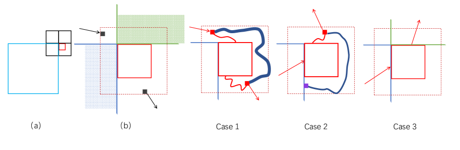
Figure 1: (a) The smallest (red) box is $\mathsf{C}$, the intermediate (black) boxes are $\mathsf{B}_{\mathrm{lt}}$, etc, and the largest (blue) box is $\mathsf{C}_{\mathrm{lb}}$. (b) lack of connectivity by $\mathsf{C}_{\mathrm{lb}}$ and $\mathsf{C}_{\mathrm{rt}}$, where the small (black) solid boxes are $\mathsf{C}_{\mathrm{enter}}$ and $\mathsf{C}_{\mathrm{exit}}$. In Case 1, the small (red) solid boxes are $\mathsf{C}_{i,1}$ and $\mathsf{C}_{i,2}$, the thin (red) curve stands for $[\mathsf{C}_{i,1},\mathsf{C}_{i,2}]$ and the thick (blue) curve stands for $\mathcal{C}_{i,\mathrm{replace}}$. In Case 2, the small bottom (purple) solid box stands for the neighbor of $\mathsf{C}_{i,1}=\mathsf{C}_{\mathrm{lb}}$ in $\mathcal{C}_{i,\mathrm{replace}}$, which may have side length less than $\epsilon^{*}s_{\mathsf{C}_{i,1}}$.

It remains to justify the above claim. We first prove it in the harder case when $\mathsf{C}_{\mathrm{large}}\subseteq\mathbb{V}^{o}$. As shown in (a) of Figure 1, let $\mathsf{B}_{\mathrm{lt}},\mathsf{B}_{\mathrm{rt}},\mathsf{B}_{\mathrm{lb}},\mathsf{B}_{\mathrm{rb}}$ be the four dyadic boxes with side length $2s_{\mathsf{C}}$ whose closures have non-empty intersection with the closure of $\mathsf{C}$; here, the subscript $\mathrm{lt}$ means “left-top’ and $\mathrm{rb}$ means “right-bottom”, etc. (Note that $\mathsf{B}_{\mathrm{lt}},\mathsf{B}_{\mathrm{rt}},\mathsf{B}_{\mathrm{lb}},\mathsf{B}_{\mathrm{rb}}$ are not necessarily cells in $\mathcal{V}_{\delta}$.) We suppose without loss of generality that $\mathsf{C}\subset\mathsf{B}_{\mathrm{r}b}$ (so that all cells in $\mathsf{B}_{\mathrm{rb}}$ have side length at most $s_{\mathsf{C}}$). If $\mathsf{B}_{\mathrm{lt}}$ is not partitioned, then denote by $\mathsf{C}_{\mathrm{lt}}$ the cell containing $\mathsf{B}_{\mathrm{lt}}$ (otherwise we define $\mathsf{C}_{\mathrm{lt}}=\emptyset$) — similarly for $\mathrm{lb},\mathrm{rt},\mathrm{rb}$. Let $\mathfrak{C}_{\mathrm{parents}}=\{\mathsf{C}_{\mathrm{lt}},\mathsf{C}_{\mathrm{rt}},\mathsf{C}_{\mathrm{lb}}\}$, noting $\mathsf{C}_{\mathrm{rb}}=\emptyset$. Note that it is possible that $\mathfrak{C}_{\mathrm{parents}}=\{\emptyset\}$. By (71) there exists a sequence $\mathcal{C}_{i,\mathrm{cross}}$ of neighboring cells with side length at least $\epsilon^{*}s_{\mathsf{C}}$, which encloses $\mathsf{C}$ and has all cells intersecting with $\mathsf{C}_{\mathrm{large}}\setminus\mathsf{C}$. Suppose that $\mathcal{C}_{i,\mathrm{cross}}$ intersects $[\mathsf{C}_{\mathrm{enter}},\mathsf{C}_{\mathrm{exit}}]_{\mathcal{C}_{i}}$ at ${\mathsf{C}}_{i,1}$ and ${\mathsf{C}}_{i,2}$. Then, $\mathcal{C}_{i,\mathrm{cross}}$ can be split two segments, with respective ending cells ${\mathsf{C}}_{i,1}$ and ${\mathsf{C}}_{i,2}$.

We first show that the interior of one of the segments does not intersect $\mathfrak{C}_{\mathrm{parents}}$. Suppose this does not hold. If $\mathsf{C}_{\mathrm{lt}}$ lies in the interior of a segment, neither $\mathsf{C}_{\mathrm{lb}}$ nor $\mathsf{C}_{\mathrm{rt}}$ lie in the interior of the other segment, because they are neighbors of $\mathsf{C}_{\mathrm{lt}}$. Then, $\mathsf{C}_{\mathrm{lb}}$ and $\mathsf{C}_{\mathrm{rt}}$ respectively lie in the interior of different segments, as shown in (b) of Figure 1. By connectivity, this implies that one of them is contained in $(\mathsf{C}_{i,1},\mathsf{C}_{i,2})_{\mathcal{C}_{i}}\subseteq(\mathsf{C}_{\mathrm{enter}},\mathsf{C}_{\mathrm{exit}})_{\mathcal{C}_{i}}$, arriving at a contradiction to the definitions of $\mathsf{C}_{\mathrm{enter}}$ and $\mathsf{C}_{\mathrm{exit}}$.

Next, we prove our claim in the following separate cases, as shown in Figure 1.

Case 1: ${\mathsf{C}}_{i,1},{\mathsf{C}}_{i,2}\notin\mathfrak{C}_{\mathrm{parents}}$. In this case we can just let $\mathcal{C}_{i,\mathrm{replace}}$ be the segment which does not contain any cell in $\mathfrak{C}_{\mathrm{parents}}$. By our assumption, we see that all cells in $\mathcal{C}_{i,\mathrm{replace}}$ have side lengths in $[\epsilon^{*}s,s]$. Therefore, $\psi(\mathcal{C}_{i,\mathrm{replace}})=\emptyset$. In addition, $\mathsf{C}\notin\mathcal{C}_{i,\mathrm{replace}}$. Thus, we have justified (i) of the claim.

Case 2: $|\{{\mathsf{C}}_{i,1},{\mathsf{C}}_{i,2}\}\cap\mathfrak{C}_{\mathrm{parents}}|=1$. In this case, we repeat the procedure as in Case 1. However, (supposing ${\mathsf{C}}_{i,1}\in\mathfrak{C}_{\mathrm{parents}}$) it is now possible that $\psi(\mathcal{C}_{i,\mathrm{replace}})=\emptyset$ or $\psi(\mathcal{C}_{i,\mathrm{replace}})=\{{\mathsf{C}}_{i,1}\}$. The former case shows (i); in the latter case, we have (ii), where $q(\mathcal{C}_{i+1})=s_{{\mathsf{C}}_{i,1}}\geq 2s_{\mathsf{C}}=2q(\mathcal{C}_{i})$.

Case 3: $\{{\mathsf{C}}_{i,1},{\mathsf{C}}_{i,2}\}\subset\mathfrak{C}_{\mathrm{parents}}$. In this case, we also have ${\mathsf{C}}_{i,1}=\mathsf{C}_{\mathrm{enter}}$ and ${\mathsf{C}}_{i,2}=\mathsf{C}_{\mathrm{exit}}$ (or with the ordering switched), and thus both ${\mathsf{C}}_{i,1}$ and ${\mathsf{C}}_{i,2}$ are neighboring to (in the sequence $\mathcal{C}_{i}$) cells of side length at most $s_{\mathsf{C}}$. By maximality of $\mathsf{C}$ in $\psi(\mathcal{C}_{i})$, we see that ${\mathsf{C}}_{i,1}$ and ${\mathsf{C}}_{i,2}$ have side lengths at most $s_{\mathsf{C}}/\epsilon^{*}$ (and at least $2s_{\mathsf{C}}$ since they are in $\mathfrak{C}_{\mathrm{parents}}$). If ${\mathsf{C}}_{i,1}$ and ${\mathsf{C}}_{i,2}$ are diagonal to each other (then they must be both neighboring $\mathsf{C}$), we let $\mathcal{C}_{i,\mathrm{replace}}$ be the sequence ${\mathsf{C}}_{i,1},\mathsf{C},{\mathsf{C}}_{i,2}$; if ${\mathsf{C}}_{i,1}$ and ${\mathsf{C}}_{i,2}$ are neighboring to each other, then we let $\mathcal{C}_{i,\mathrm{replace}}$ be the sequence ${\mathsf{C}}_{i,1},{\mathsf{C}}_{i,2}$. In both cases, we have $\psi(\mathcal{C}_{i,\mathrm{replace}})=\emptyset$, justifying (i).

We next consider the easier case that $\mathsf{C}$ intersects $\partial\mathbb{V}$. In this case, $\mathfrak{C}_{\mathrm{parents}}$ contains at most one cell in $\mathbb{V}$ and we are either in Case 1 or Case 2. Following similar (and slightly simpler) analysis to the one above then yields the proof of the claim in this case. Altogether, this completes the verification of the claim, and thus completes the proof of the lemma. ∎

3.3 Concentration of the distances

In this section we show the following concentration result on the Liouville graph distance. Recall the constant $C_{\mathrm{Mc}}$ specified in Lemma 3.1.

Proposition 3.17.

For any fixed $0<\xi<C_{\mathrm{Mc}}/3$ there exists a constant $c=c(\gamma,\xi)$ so that for any sequence of $\xi$-admissible pairs $(A_{\delta},B_{\delta})$ we have that for any $\iota\in(0,1)$,

$$|\log\min_{x\in A_{\delta},y\in B_{\delta}}D_{\gamma,\delta}(x,y)-{\mathbb{E}}\log\min_{x\in A_{\delta},y\in B_{\delta}}D_{\gamma,\delta}(x,y)|\leq\iota\log\delta^{-1}\ \mbox{\rm with $c\cdot\iota^{2}$-high probability}\,.$$ (73)

In addition, with probability at least $1-e^{-(\log\delta^{-1})^{0.7}}$, we have that

$$|\log\min_{x\in A_{\delta},y\in B_{\delta}}D_{\gamma,\delta}(x,y)-{\mathbb{E}}\log\min_{x\in A_{\delta},y\in B_{\delta}}D_{\gamma,\delta}(x,y)|\leq(\log\delta^{-1})^{0.95}\,.$$ (74)

Furthermore, (73) and (74) hold with $D_{\gamma,\delta}$ replaced with $D_{\gamma,\delta,\eta}$.

Proof.

We first give a detailed proof of (73) and then sketch the necessary minor adaptations needed in order to obtain (74). For both (73) and (74), we will only provide a proof in the case of $A=\{u\}$ and $B=\{v\}$, as the general case follows by the same proof with minimal change — the assumption of admissible pairs is required only in order to be able to apply Proposition 3.2 and Lemma 3.5. Also, provided with (73) and (74), the fact that (73) and (74) hold with $D_{\gamma,\delta}$ replaced with $D_{\gamma,\delta,\eta}$ follows from Lemma 2.7, Corollary 3.9 and Lemma 3.8.

Proof of (73). It is obvious from Proposition 3.2 and Corollary 3.3 that (73) is equivalent to the statement that with $c\cdot\iota^{2}$-high probability

$$|\frac{\log D^{\prime}_{\gamma,\delta}(u,v)}{\log\delta^{-1}}-{\mathbb{E}}\frac{\log D^{\prime}_{\gamma,\delta}(u,v)}{\log\delta^{-1}}|\leq\iota\,.$$ (75)

Thus, it suffices to prove the concentration for either of the two distances. The natural attempt to prove Proposition 3.17 is to verify the Lipschitz condition for the Liouville graph distance (viewed as a function on a Gaussian process) and then apply a Gaussian concentration inequality. However, while the Lipschitz condition for the Liouville graph distance can be verified, the maximal individual variance for the Gaussian variables involved in the definition of the Liouville graph distance is infinite. On the other hand, while the maximal individual variance for the Gaussian variables involved in the definition of the approximate Liouville graph distance can be controlled, the Lipschitz condition does not hold in an obvious way. In order to see the failing of the Lipschitz condition, note that one can perturb the Gaussian process such that in constructing $\mathcal{V}_{\delta}$, a cell that was not further partitioned in the original environment would now be further partitioned. Once this extra partitioning occurs, it is possible (but unlikely) that these sub-cells would be further partitioned into arbitrarily small Euclidean squares. (Indeed, the decision concerning further partitioning depends on random variables which are independent from those determining the original partition.) In order to address this issue, we will employ the Lipschitz condition for the Liouville graph distance and the control on the maximal individual variance for the Gaussian variables involved in the approximate Liouville graph distance, and use Proposition 3.2 to make a connection between these two distances.

We consider the Gaussian space generated by the collection $\{(\eta_{\delta}(v),\tilde{h}_{\delta}(v))\}_{v\in\mathbb{V},\delta>0}$, see (11) and (13). For $\delta>0$, let $\mathbf{X}_{\delta}$ denote the subspace spanned by $\{(\eta_{\epsilon}(v),\tilde{h}_{\epsilon}(v)):v\in\mathbb{V},\epsilon\geq\delta^{C_{\mathrm{mc}}}\}$. Let $\mathbf{Y}_{\delta}$ denote the subspace orthogonal to $\mathbf{X}_{\delta}$, and note that it is generated by the white noise $W(dw,ds)$ for $s<\delta^{2C_{\mathrm{mc}}}$). For $\delta^{\prime}<\delta^{C_{\mathrm{mc}}}$ we write the orthogonal decomposition

$$(\eta_{\delta^{\prime}}(\cdot),\tilde{h}_{\delta^{\prime}}(\cdot))=(\eta_{\delta^{C_{\mathrm{mc}}}}(\cdot),\tilde{h}_{\delta^{C_{\mathrm{mc}}}}(\cdot))+(\eta^{\perp}_{\delta,\delta^{\prime}}(\cdot),\tilde{h}^{\perp}_{\delta,\delta^{\prime}}(\cdot))=:{\cal X}_{\delta}+{\cal Y}_{\delta,\delta^{\prime}},$$

where ${\cal Y}_{\delta,\delta^{\prime}}(\cdot)$ is measurable on $\mathbf{Y}_{\delta}$. (Possible configurations of $\cal X$ and $\cal Y$ will be denoted by $\bf x$ and $\bf y$. We use ${\bf x}_{\delta}$ and ${\bf y}_{\delta,\delta^{\prime}}$ as convenient shorthand notation, and we further use ${\bf y}_{\delta}$ to denote the collection ${\bf y}_{\delta,\delta^{\prime}}$ for $\delta^{\prime}<\delta^{C_{\mathrm{mc}}}$.) Denote by $M_{\gamma,\mathbf{x}_{\delta}}$ the LQG measure of the GFF on the realization $(\mathbf{x}_{\delta},{\cal Y}_{\delta})$. We apply a similar convention for $M_{\gamma,\mathbf{x}^{\prime}_{\delta}}$, $D_{\gamma,\delta,\mathbf{x}_{\delta}}(u,v)$, etc. We note that, by definition, $D^{\prime}_{\gamma,\delta}(u,v)=D^{\prime}_{\gamma,\delta,\mathcal{X}_{\delta}}(u,v)$. Furthermore, $D^{\prime}_{\gamma,\delta,\mathbf{x}_{\delta}}(u,v)$ is a real number if each cell has side length larger than $\delta^{C_{\mathrm{mc}}}$, since then $D^{\prime}_{\gamma,\delta}$ does not depend on $\mathcal{Y}_{\delta}$. Next, we are going to show that $\log D^{\prime}_{\gamma,\delta,\mathbf{x}_{\delta}}(u,v)-\log D^{\prime}_{\gamma,\delta,\mathbf{x}^{\prime}_{\delta}}(u,v)$ is bounded by $O(1)\|\mathbf{x}_{\delta}-\mathbf{x}^{\prime}_{\delta}\|_{\infty}$, see (76) below.

Let $\mathcal{A}_{\delta}$ be such that $\{\mathcal{X}_{\delta}\in\mathcal{A}_{\delta}\}=\{\mbox{each cell in }\mathcal{V}_{\delta}\mbox{ has side length at least }\delta^{C_{\mathrm{mc}}}\}$. Let $\iota$ be an arbitrarily small positive number and $\alpha>0$, and let $\mathcal{E}^{*}_{\delta,\iota,\alpha}=\{({\cal X}_{\delta},{\cal Y}_{\delta})\in\tilde{\mathcal{E}}^{*}_{\delta,\iota,\alpha}\}$ be the event such that

$$|\frac{\log D_{\gamma,\delta^{\prime}}(u,v)}{\log\delta^{-1}}-\frac{\log D^{\prime}_{\gamma,\delta^{\prime\prime}}(u,v)}{\log\delta^{-1}}|\leq\iota/4\mbox{ for all }\delta^{1+\iota/\alpha}\leq\delta^{\prime},\delta^{\prime\prime}\leq\delta^{1-\iota/\alpha}.$$

It will be convenient in what follows to write

$$\mathcal{E}^{*}_{\delta,\iota,\alpha,\mathbf{x}_{\delta}}=\{\bf y_{\delta}:(\bf x_{\delta},\bf y_{\delta})\in\tilde{\mathcal{E}}^{*}_{\delta,\iota,\alpha}\}.$$

By Proposition 3.2 and Lemmas 3.1 and 3.5, we can choose an $\alpha>0$ depending only on $\gamma$, such that for any arbitrarily small $\iota>0$, $\mathcal{E}^{*}_{\delta,\iota,\alpha}$ occurs with $c\cdot\iota$-high probability. As a result, we see that there exists a set $\mathcal{A}\subseteq\mathcal{A}_{\delta}$ such that

$${\mathbb{P}}(\mathcal{E}^{*}_{\delta,\iota,\alpha}\mid\mathbf{X}_{\delta})\geq 0.9\mbox{ on the event }{\cal X}_{\delta}\in\mathcal{A},\mbox{which occurs with $c\cdot\iota$-high probability}\,.$$

In particular, for ${\bf x}_{\delta},{\bf x}_{\delta}^{\prime}\in\mathcal{A}$, $\mathcal{E}^{*}_{\delta,\iota,\alpha,\mathbf{x}_{\delta}}\cap\mathcal{E}^{*}_{\delta,\iota,\alpha,\mathbf{x}_{\delta}^{\prime}}$ is non-empty.

Let $\ell=\|\mathbf{x}_{\delta}-\mathbf{x}^{\prime}_{\delta}\|_{\infty}$. We see from Lemma 3.8 that as long as $\ell\leq\ell_{\delta}=\frac{\iota\log\delta^{-1}}{2\gamma\alpha}$ we have

$$D_{\gamma,\delta^{1-\iota/\alpha},\mathbf{x}_{\delta}}(u,v)\leq D_{\gamma,\delta,\mathbf{x}^{\prime}_{\delta}}(u,v)\leq D_{\gamma,\delta^{1+\iota/\alpha},\mathbf{x}_{\delta}}(u,v)\,.$$

(Note that the above is an inequality between random variables that depend on ${\cal Y}_{\delta}$, which holds for almost all configurations $\mathbf{y}_{\delta}$.) Consequently, on the event ${\cal Y}_{\delta}\in\mathcal{E}^{*}_{\delta,\iota,\alpha,\mathbf{x}_{\delta}}\cap\mathcal{E}^{*}_{\delta,\iota,\alpha,\mathbf{x}_{\delta}^{\prime}}$ we have $|\log D_{\gamma,\delta,\mathbf{x}^{\prime}_{\delta}}(u,v)-\log D_{\gamma,\delta,\mathbf{x}_{\delta}}(u,v)|\leq\frac{1}{2}\iota\log\delta^{-1}$ and thus,

$$|\log D^{\prime}_{\gamma,\delta,\mathbf{x}^{\prime}_{\delta}}(u,v)-\log D^{\prime}_{\gamma,\delta,\mathbf{x}_{\delta}}(u,v)|\leq\iota\log\delta^{-1}\,.$$ (76)

Recall that, for all $\mathbf{x}_{\delta}$, $D^{\prime}_{\gamma,\delta,\bf x_{\delta}}$ does not depend on ${\cal Y}_{\delta}$. Then, we have deduced that (76) holds for all $\bf x_{\delta},\bf x^{\prime}_{\delta}\in\mathcal{A}$ satisfying $\ell\leq\ell_{\delta}$.

At this point, we are ready to deduce our concentration result. Let $d^{\prime}_{u,v}$ be the minimal number such that

$${\mathbb{P}}({\cal X}_{\delta}\in\mathcal{A}^{\prime})\geq 1/2\,,\mbox{ where }\mathcal{A}^{\prime}=\{\mathbf{x}_{\delta}\in\mathcal{A}:D^{\prime}_{\gamma,\delta,\mathbf{x}_{\delta}}(u,v)\leq d^{\prime}_{u,v}\}\,.$$

Note that the above is well defined since when $\mathbf{x}_{\delta}\in\mathcal{A}$, we have that $D^{\prime}_{\gamma,\delta,\mathbf{x}_{\delta}}(u,v)$ is a measurable function of $\mathbf{x}_{\delta}$. Recalling (76), we see that for $c=c(\gamma)>0$

$${\mathbb{P}}(\log D^{\prime}_{\gamma,\delta}(u,v)\geq\log d^{\prime}_{u,v}+\iota\log\delta^{-1})\leq{\mathbb{P}}(\mathcal{X}_{\delta}\not\in\mathcal{A})+{\mathbb{P}}(\min_{\mathbf{x}_{\delta}^{\prime}\in\mathcal{A}^{\prime}}\|{\mathcal{X}_{\delta}}-\mathbf{x}^{\prime}_{\delta}\|_{\infty}\geq\ell_{\delta})\leq\delta^{c\iota^{2}}\,,$$ (77)

where in the last step we have used Lemma 2.1, as well as the fact that maximal individual variance of the random variables in ${\mathcal{X}}_{\delta}$ is $O_{C_{\mathrm{mc}}}(\log\delta^{-1})$.

By a similar reasoning, we can also get that

$${\mathbb{P}}(\log D^{\prime}_{\gamma,\delta}(u,v)\leq\log d^{\prime}_{u,v}-\iota\log\delta^{-1})\leq\delta^{c\iota^{2}}\,.$$ (78)

Due to the uniform square integrability of $\log D^{\prime}_{\gamma,\delta}(u,v)/\log(1/\delta)$, which follows from $|D^{\prime}_{\gamma,\delta}|\leq|\mathcal{V}_{\delta}|$ and the reasoning in Lemma 3.1, we conclude from (77) and (78) that $|{\mathbb{E}}\log D^{\prime}_{\gamma,\delta}(u,v)-\log d^{\prime}_{u,v}|\leq 2\iota\log\delta^{-1}$. Combined with (77) and (78), this completes the proof of (75) (we adjust the value of $\iota$ appropriately).

Proof of (74). We now sketch the necessary modifications in order to prove (74). For simplicity of exposition, in what follows we will repeatedly use higher powers of $\log\delta^{-1}$ to absorb error terms with lower powers of $\log\delta^{-1}$. It is obvious from Proposition 3.2 and Corollary 3.3 that (74) can be deduced from the statement that with probability at least $1-e^{(\log\delta^{-1})^{0.8}}$,

$$|\log D^{\prime}_{\gamma,\delta}(u,v)-{\mathbb{E}}\log D^{\prime}_{\gamma,\delta}(u,v)|\leq(\log\delta^{-1})^{0.94}\,.$$ (79)

To prove (79), we follow the proof of (73), but in place of $\mathcal{E}^{*}_{\delta,\iota,\alpha}$ we define $\mathcal{E}^{*}_{\delta,\alpha}$ to be the event that

$$|\frac{\log D_{\gamma,\delta^{\prime}}(u,v)}{\log\delta^{-1}}-\frac{\log D^{\prime}_{\gamma,\delta^{\prime\prime}}(u,v)}{\log\delta^{-1}}|\leq(\log\delta^{-1})^{-0.09}\mbox{ for all }\delta e^{-\alpha^{-1}(\log\delta^{-1})^{0.9}}\leq\delta^{\prime},\delta^{\prime\prime}\leq\delta e^{\alpha^{-1}(\log\delta^{-1})^{0.9}}.$$

By Proposition 3.2 and Lemmas 3.1 and 3.5, we can choose an $\alpha>0$ depending only on $\gamma$, such that ${\mathbb{P}}(\mathcal{E}^{*}_{\delta,\alpha})\geq 1-\delta^{1/\alpha}$. As a result, we see that there exists a set $\mathcal{A}\subseteq\mathcal{A}_{\delta}$ such that

$${\mathbb{P}}(\mathcal{E}^{*}_{\delta,\alpha}\mid\mathbf{X}_{\delta})\geq 0.9\mbox{ on the event }{\cal\mathcal{X}_{\delta}}\in\mathcal{A},\mbox{ and }{\mathbb{P}}(\mathcal{X}_{\delta}\in\mathcal{A}\mbox{)}\geq 1-\delta^{\frac{1}{2\alpha}}\,.$$

At this point, we can repeat the analysis as for (73) and deduce that for $\ell_{\delta}=(\log\delta^{-1})^{0.9}$

$${\mathbb{P}}(\log D^{\prime}_{\gamma,\delta}(u,v)\geq\log d^{\prime}_{u,v}+(\log\delta^{-1})^{0.95})\leq{\mathbb{P}}(\mathcal{X}_{\delta}\not\in\mathcal{A})+{\mathbb{P}}(\min_{\mathbf{x}_{\delta}^{\prime}\in\mathcal{A}^{\prime}}\|\mathcal{X}_{\delta}-\mathbf{x}^{\prime}_{\delta}\|_{\infty}\geq\ell_{\delta})\leq e^{-\Omega((\log\delta^{-1})^{0.8})}\,,$$

where in the last step we again have used Lemma 2.1, as well as the fact that the maximal individual variance of the random variables in $\mathcal{X}_{\delta}$ is $O_{C_{\mathrm{mc}}}(\log\delta^{-1})$. The proof of the lower deviation in (79) is similar, leading to (79) and thus completing the proof of (74). ∎

4 Liouville heat kernel

In this section, we relate the Liouville heat kernel to the Liouville graph distance.

4.1 Lower bound

In this section, we provide a lower bound on the Liouville heat kernel in terms of the Liouville graph distance. For $u,v\in\mathbb{V}$, we denote

$$\chi^{+}_{u,v}=\limsup_{\delta\to 0}\frac{{\mathbb{E}}\log D_{\gamma,\delta}(u,v)}{\log\delta^{-1}}\,.$$

Recalling Lemma 2.12, we see that $0<\chi^{+}_{u,v}<1$. We will show that there exists a finite random variable $C>0$ (measurable with respect to the GFF, and depending on $u,v$) such that for all $t\in(0,1]$,

$$\mathsf{p}_{t}^{\gamma}(u,v)\geq C\exp\Big{\{}-t^{-\frac{\chi^{+}_{u,v}}{2-\chi^{+}_{u,v}}+o(1)}\Big{\}}\,.$$ (80)

In order to prove (80), it suffices to show that there exists a $t_{0}>0$ (deterministic) so that for any arbitrarily small and fixed $\iota>0$, there exists a small positive random variable $c=c_{\gamma,u,v,\iota}>0$, measurable on the GFF, such that for all $t\in(0,t_{0}]$, the following holds: with probability at least $1-e^{-(\log t^{-1})^{0.2}}$,

$$\mathsf{p}_{s}^{\gamma}(u,v)\geq c\exp\Big{\{}-t^{-\frac{\chi^{+}_{u,v}}{2-\chi^{+}_{u,v}}-\iota}\Big{\}}\mbox{ for all }t\leq s\leq 2t\,.$$ (81)

Indeed, (81) yields (80) for $t\leq t_{0}$ by an application of the Borel-Cantelli lemma for times $t_{i}=2^{-i}$. On the other hand, (80) holds for $t>t_{0}$ by the Markov property and multiple applications of [25, Corollary 5.20].

To show (81), fix an arbitrarily small $\iota>0$ and let $\delta=t^{{1}/(2-\chi^{+}_{u,v})+\iota}$. Also, throughout the section, we use $\hat{\mathsf{C}}$ to denote a cell in $\mathcal{V}_{\delta}$, while $\mathsf{C}$ will stand for the boxes $\{B_{i}\}$ in Lemma 3.13.

A natural approach to proving (81) is to show that with not too small probability, the Liouville Brownian motion can cross each cell in $\mathcal{V}_{\delta}$ without accumulating too much “Liouville time” (i.e., the PCAF as defined in (1)), provided with which one can then force the SBM to travel along the geodesic between $u$ and $v$ in $\mathcal{V}_{\delta}$. However, there is a substantial obstacle due to the the possibility that two neighboring cells along the geodesic may have side lengths differing by a factor as large as a power in $\delta$. This is further complicated by a technical challenge: for a cell $\hat{\mathsf{C}}\in\mathcal{V}_{\delta}$, the Liouville time accumulated during traveling through $\hat{\mathsf{C}}$ depends on the starting and ending points, and we do not expect uniform bounds on that.

We now discuss how to address these challenges; a crucial role is played by Lemma 3.13. We work on the event $\mathcal{E}_{1}$ defined as

$$\mathcal{E}_{1}=\mathcal{E}_{\delta,\alpha^{*}}\cap\mathcal{E}_{\delta,\alpha^{*},u,v}\cap\{\mbox{\rm\eqref{eq-tilde-h-eta-assump} holds}\}\,,$$ (82)

where $\mathcal{E}_{\delta,\alpha^{*}}$ and $\mathcal{E}_{\delta,\alpha^{*},u,v}$ are defined in (39) and (65), respectively. Note that ${\mathbb{P}}(\mathcal{E}_{1})\geq 1-e^{-(\log\delta^{-1})^{0.24}}$, by Lemmas 3.4, 3.12 and the discussion above (52). We next will extract a sequence of neighboring boxes using Lemma 3.13. To ensure more desirable properties of this sequence of boxes, we will work on a more restricted event than $\mathcal{E}_{1}$. By Propositions 3.2 and 3.17, we see that with $c\cdot\iota^{2}$-high probability, $D^{\prime}_{\delta,\gamma}(u,v)\leq\delta^{-\chi^{+}_{u,v}-\frac{1}{4}(2-\chi^{+}_{u,v})^{2}\cdot\iota}$. Setting

$$\mathcal{E}_{2}=\mathcal{E}_{1}\cap\{D^{\prime}_{\delta,\gamma}(u,v)\leq\delta^{-\chi^{+}_{u,v}-\frac{1}{4}(2-\chi^{+}_{u,v})^{2}\cdot\iota}\}\cap\{\mbox{the event in \eqref{Eq.error-coarse-fine}}\},$$ (83)

we deduce, using arguments similar to those employed in the proof of Lemma 3.4, that with high probability we have

$$\max_{\hat{\mathsf{C}}\in\mathcal{V}_{\delta}}\max_{x\in\mathbb{V}\cap\hat{\mathsf{C}}_{\mathrm{large}}}|\eta_{(\epsilon^{*})^{2}s_{\hat{\mathsf{C}}}}^{s_{\hat{\mathsf{C}}}}(x)|\leq(\log\delta^{-1})^{0.8}.$$ (84)

and therefore, ${\mathbb{P}}(\mathcal{E}_{2})\geq 1-e^{-(\log\delta^{-1})^{0.23}}$.

We work on $\mathcal{E}_{2}$ in what follows. Denote the sequence $\{B_{i}\}$ provided in Lemma 3.13 by $\mathcal{C}=(\mathsf{C}_{1},\ldots,\mathsf{C}_{d})$; recall that this sequence is measurable with respect to $\mathcal{V}_{\delta}$, and joins $u$ to $v$. Then, $d\leq\delta^{-\chi^{+}_{u,v}-\frac{1}{2}(2-\chi^{+}_{u,v})^{2}\cdot\iota}$, and each $\mathsf{C}_{i}$ satisfies $M_{\gamma,s_{\mathsf{C}_{i}}}(\mathsf{C}_{i})\leq\delta^{2}e^{O((\log\delta^{-1})^{0.8})}$ (recall (84) and that $s_{\mathsf{C}_{i}}=(\epsilon^{*})^{2}s_{\hat{\mathsf{C}_{i}}}$, where $\hat{\mathsf{C}_{i}}$ is the cell containing $\mathsf{C}_{i}$, see Lemma 3.13). Furthermore, the law of $\{\eta_{\delta^{\prime}}^{s_{\mathsf{C}_{i}}}(x):\delta^{\prime}<s_{\mathsf{C}_{i}},x\in(\mathsf{C}_{i})_{\mathrm{large}}\mbox{ for some }\mathsf{C}_{i}\in\mathcal{C}\}$ conditioned on $\mathcal{V}_{\delta}$ coincides with its unconditional version. (Here, we abuse notation by using $\mathsf{C}_{i}$ to denote a dyadic box which is not necessarily a cell. The abuse of notation is justified by the fact that $M_{\gamma,s_{\mathsf{C}_{i}}}(\mathsf{C}_{i})\leq\delta^{2}e^{O((\log\delta^{-1})^{0.8})}$ and thus the $\mathsf{C}_{i}$’s will essentially play the role of cells.) For $i=1,\ldots,d-1$, denote for brevity $s_{i}:=s_{\mathsf{C}_{i}}$ and write $\Lambda_{i}=\partial\mathsf{C}_{i}\cap\partial\mathsf{C}_{i+1}$. We emphasize that the $\Lambda_{i}$’s are measurable with respect to $\mathcal{V}_{\delta}$. As discussed above, we will force the SBM to travel through $\mathsf{C}_{1},\ldots,\mathsf{C}_{d}$ sequentially, and will show that this occurs with high enough probability. To this end, we will crucially use the fact $\mathcal{C}$ is a good sequence, and thus

$$\mathcal{L}_{1}(\Lambda_{i}),\mathcal{L}_{1}(\Lambda_{(i-1)\vee 1})\geq\epsilon^{*}s_{i}\mbox{ for }1\leq i<d\,.$$ (85)

Here $\mathcal{L}_{1}$ is the 1-dimensional Lebesgue measure, and $\epsilon^{*}$ is defined in (64).

Consider $2\leq i\leq d-1$. For $\mathsf{C}_{i}\in\mathcal{C}$ and $z\in\mathsf{C}_{i}$, we say that $z$ is a fast point (with respect to $\mathsf{C}_{i}$) if for any $\Lambda\subseteq\Lambda_{i}$ such that $\mathcal{L}_{1}(\Lambda)\geq 0.1\mathcal{L}_{1}(\Lambda_{i})$ one has

$$P_{z}(F(\sigma_{\Lambda})\leq\delta^{2}C_{\delta})\geq\exp\{-\exp\{(\log\delta^{-1})^{2/3}\}\}=:p_{\mathrm{fast}}(=\exp\{-(1/\delta)^{o(1)}\})\,,$$ (86)

where $\sigma_{\Lambda}$ is the first time when the SBM hits $\Lambda$ and

$$C_{\delta}=\exp\{(\log\delta^{-1})^{0.95}\}(=(1/\delta)^{o(1)})\,.$$ (87)

Note that we allow $z\in\partial\mathsf{C}_{i}$, however the fact that being fast involves considering all possible $\Lambda$ makes the notion non-trivial even for a point $z\in\partial\mathsf{C}_{i}$, since we need to consider sets $\Lambda$ with $z\not\in\Lambda$. We say that $\mathsf{C}_{i}$ is fast if

$$\mathcal{L}_{1}(\Lambda_{i-1,\mathrm{fast}})\geq 0.1\mathcal{L}_{1}(\Lambda_{i-1})\mbox{ where }\Lambda_{i-1,\mathrm{fast}}=\{z\in\mathsf{\Lambda}_{i-1}:z\mbox{ is fast\ with respect to $\mathsf{C}_{i}$}\}\,.$$ (88)

A crucial ingredient for the proof of (81) is the proof that with high probability all the $\mathsf{C}_{i}$’s are fast simultaneously. To this end, we now estimate the probability that a particular $\mathsf{C}_{i}$ is fast. (We will later apply a union bound.)

Lemma 4.1.

There exists a $\delta_{0}>0$ such that for all $\delta<\delta_{0}$ there exists an event $\mathcal{E}_{3}$ of high probability such that the following holds. For each $2\leq i\leq d-1$ there exists an event $\mathcal{E}_{\mathsf{C}_{i}}$ such that

$${\mathbb{P}}(\mathcal{E}_{\mathsf{C}_{i}}\mid\mathcal{V}_{\delta})\geq 1-\exp\{-2^{\sqrt{\log\delta^{-1}}}\}\mbox{ and }(\mathcal{E}_{\mathsf{C}_{i}}\cap\mathcal{E}_{3})\subset\{\mathsf{C}_{i}\mbox{ is fast}\}.$$

(The event $\mathcal{E}_{3}$ is defined in (92) below.)

We begin our preparation for the proof of Lemma 4.1. Since our goal is to show that with very high probability $\mathsf{C}_{i}\in\mathcal{C}$ is fast, a first (or second) moment computation will not be enough. Instead, we will use a simple multi-scale analysis and employ a percolation argument. We first introduce some definitions. Set $k=\lfloor(\log\delta^{-1})^{0.51}\rfloor$ and $K=2^{k}$. Take $\mathsf{C}\in\mathcal{C}$ and partition it into $K^{2}$ many dyadic squares with side length $s_{\mathsf{C}}/K$. Denote the collection of these boxes by $\mathcal{B}_{\mathsf{C}}$, and denote by $\mathsf{B}_{\mathrm{large}}$ (respectively, $\mathsf{B}_{\mathrm{Large}}$) the boxes concentric with $\mathsf{B}$ but with double (respectively, triple) side length. For a fixed $\mathsf{B}\in\mathcal{B}_{\mathsf{C}}$ and $z\in\mathsf{B}$, we say that $z$ is a pre-fast point with respect to the box $\mathsf{B}$ if for any $\Lambda\subseteq\partial\mathsf{B}$ with $\mathcal{L}_{1}(\Lambda)\geq 10^{-5}s_{\mathsf{C}}/K$ one has

$$P_{z}(F(\sigma_{\Lambda})\leq\delta^{2}C_{\delta}K^{-4};\sigma_{\Lambda}\leq\sigma_{\partial\mathsf{B}_{\mathrm{Large}}})\geq\exp\{-(\log\delta^{-1})^{1/10}\}\,.$$ (89)

Note that the notions of pre-fast and fast are related, but one does not necessarily imply the other. We say that $\mathsf{B}$ is pre-fast if the subset of pre-fast points with respect to $\mathsf{B}$ on $\partial\mathsf{B}$ has 1-dimensional Lebesgue measure at least $(1-10^{-5})\mathcal{L}_{1}(\partial\mathsf{B})$. By definition, the property of boxes being pre-fast has long range correlation, though we expect that the correlation decays quickly.

Figure 2: In the left picture, the (black) boxes stand for (a piece of) the sequence of good cells joining $u$ and $v$. The (red) line stands for the good sequence of boxes $\{\mathsf{B}_{i}\}$ in Lemma 3.13, which are denoted by $\{\mathsf{C}_{i}\}$ now. The right picture is a zoom in, where the big (red) box is $\mathsf{C}=\mathsf{C}_{i}$, and the small (blue) boxes form $\mathcal{B}_{\mathsf{C}}$.

In order to control the correlation, we define a field $\tilde{\eta}^{\mathsf{B}}:=\{\tilde{\eta}_{\epsilon^{\prime}}^{\mathsf{B},s_{\mathsf{C}}}(z):\epsilon^{\prime},z\}$ by

$$\tilde{\eta}_{\epsilon^{\prime}}^{\mathsf{B},s_{\mathsf{C}}}(z):=\left\{\begin{array}[]{ll}\sqrt{\pi}\int_{\mathbb{V}\times((\epsilon^{\prime})^{2},s_{\mathsf{C}}^{2})}p_{{}_{\mathsf{B}_{\mathrm{Large}}}}(s/2;z,w)W(dw,ds),&\mbox{if }z\in\mathsf{B}_{\mathrm{large}}\mbox{ and }\epsilon^{\prime}<s_{\mathsf{C}},\\ 0,&\mbox{otherwise,}\end{array}\right.$$ (90)

where $p_{{}_{\mathsf{B}_{\mathrm{Large}}}}(s/2;z,w)$ is the transition density for SBM truncated upon exiting the box $\mathsf{B}_{\mathrm{Large}}$. A derivation similar to (52) yields that with high probability we have

$$\max_{\mathsf{C}\in\mathcal{C}}\max_{\mathsf{B}\in\mathcal{B}_{\mathsf{C}},z\in\mathsf{B}_{\mathrm{large}}}\ \max_{\epsilon^{\prime}<s_{\mathsf{C}},\log_{2}\epsilon^{\prime}\in\mathbb{Z}}|\tilde{\eta}_{\epsilon^{\prime}}^{\mathsf{B},s_{\mathsf{C}}}(z)-\eta_{\epsilon^{\prime}}^{s_{\mathsf{C}}}(z)|=O(\sqrt{\log\delta^{-1}})\,.$$ (91)

With $\mathcal{E}_{2}$ as in (83), let $\mathcal{E}_{3}$ be defined by

$$\mathcal{E}_{3}=\mathcal{E}_{2}\cap\{\mbox{the event in \eqref{eq-assumption-in-lower-heat-kernel} holds }\}\,.$$ (92)

Since ${\mathbb{P}}(\mathcal{E}_{2})\geq 1-e^{-(\log\delta^{-1})^{0.23}}$, we have that ${\mathbb{P}}(\mathcal{E}_{3})\geq 1-e^{-(\log\delta^{-1})^{0.22}}$; in the sequel, we work on ${\mathcal{E}}_{3}$. For a SBM $X_{\cdot}$ started at a point $z$ in $\mathsf{B}$, define

$$\tilde{F}_{\mathsf{B}}(r):=\lim_{n\to\infty}\int_{0}^{r}\exp\{\gamma\tilde{\eta}_{2^{-n}}^{\mathsf{B},s_{\mathsf{C}}}(X_{r^{\prime}})-\frac{\gamma^{2}}{2}{\rm Var}(\tilde{\eta}_{2^{-n}}^{\mathsf{B},s_{\mathsf{C}}}(X_{r^{\prime}}))\}dr^{\prime},$$ (93)

where the existence of the limit follows from the same martingale argument yielding the existence of the original PCAF (see [20]). On the event ${\mathcal{E}}_{3}$ we work on, for any stopping time $\tau$ so that $X_{r}\in\mathsf{B}_{\mathrm{large}}$ for all $0\leq r\leq\tau$, we have

$$F(\tau)\leq\tilde{F}_{\mathsf{B}}(\tau)\delta^{2}s_{\mathsf{C}}^{-2}\exp\{(\log\delta^{-1})^{0.91}\}\,.$$ (94)

We note that $\tilde{F}_{\mathsf{B}}(r)$ is measurable with respect to the SBM $X.$ and the field $\tilde{\eta}^{\mathsf{B}}$, for which Lemma 3.13 is also valid (see (66) and note that $\mathsf{B}_{\mathrm{large}}\subset\mathsf{C}_{\mathrm{large}}$). The following lemma is the key to the proof of Lemma 4.1. It in particular implies that the events that geometrically separated boxes are pre-fast stochastically dominate a sequence of i.i.d. Bernoulli indicators. In what follows, we denote for brevity $\mathcal{B}_{i}:=\mathcal{B}_{\mathsf{C}_{i}}$.

Lemma 4.2.

For $\mathsf{B}\in\mathcal{B}_{i}$, there exists an event $\mathcal{E}_{\mathsf{B},\mathrm{prefast}}$ which is measurable with respect to the field $\tilde{\eta}^{\mathsf{B}}$, such that

$${\mathbb{P}}(\mathcal{E}_{\mathsf{B},\mathrm{prefast}}\mid\mathcal{V}_{\delta})\geq 1-O(K^{-2})\mbox{ and }(\mathcal{E}_{\mathsf{B},\mathrm{prefast}}\cap\mathcal{E}_{3})\subseteq\{\mathsf{B}\mbox{ is pre-fast}\}\,.$$

Proof.

Let $\mathsf{B}_{\mathrm{small}}$ denote the box concentric with $\mathsf{B}$, of half the side length. Let $\sigma_{\partial\mathsf{B}_{\mathrm{small}}}$ (respectively $\sigma_{\partial\mathsf{B}_{\mathrm{large}}}$) be the hitting time of $\partial\mathsf{B}_{\mathrm{small}}$ (respectively, $\partial\mathsf{B}_{\mathrm{large}}$) by the SBM. Let $\tau$ be the first hitting time of $\partial{\mathsf{B}}$ after $\sigma_{\partial\mathsf{B}_{\mathrm{small}}}$. Define $\mathcal{E}=\{\sigma_{\partial\mathsf{B}_{\mathrm{small}}}\leq\sigma_{\partial\mathsf{B}_{\mathrm{large}}},\tau\leq s_{i}^{2}K^{-2}\}$. From standard properties of the SBM we have that that $P(\mathcal{E})\geq 10^{-4}$ and that

$$P_{z}(X_{\tau}\in\Lambda\mid\mathcal{E})\geq 10^{-10}\,,$$ (95)

for any $z\in\partial\mathsf{B}$ and $\Lambda\subseteq\partial\mathsf{B}$ with 1-dimensional Lebesgue measure $\mathcal{L}_{1}(\Lambda)\geq 10^{-5}s_{i}/K$. Write $\tilde{F}$ for $\tilde{F}_{\mathsf{B}}$. A straightforward computation yields that

$$\mathbb{E}(E_{z}(\tilde{F}(\tau)\mid\mathcal{E})\mid\mathcal{V}_{\delta})\leq 10^{4}E_{z}\mathbb{E}(\tilde{F}(s_{i}^{2}K^{-2})\mid\mathcal{V}_{\delta})\leq 10^{4}s_{i}^{2}K^{-2}\,,$$

where we used Lemma 3.13 for $\tilde{\eta}^{\mathsf{B}}$ in the second inequality. Therefore, by Markov’s inequality, we see that

$${\mathbb{P}}(P_{z}(\tilde{F}(\tau)\geq s_{i}^{2}\mid\mathcal{E})\geq 10^{-11}\mid\mathcal{V}_{\delta})\leq O(K^{-2})\,.$$

Combining the preceding inequality with (95) and using the fact that

$$P_{z}(\tilde{F}(\tau)\leq{s_{i}^{2}},X_{\tau}\in\Lambda,\mathcal{E})\geq P_{z}(\mathcal{E})(P_{z}(X_{\tau}\in\Lambda\mid\mathcal{E})-P_{z}(\tilde{F}(\tau)\geq s_{i}^{2}\mid\mathcal{E}))\,,$$

we get that for any $\Lambda\subseteq\partial\mathsf{B}$ with $\mathcal{L}_{1}(\Lambda)\geq 10^{-5}s_{i}/K$

$${\mathbb{P}}(P_{z}(\tilde{F}(\tau)\leq s_{i}^{2},X_{\tau}\in\Lambda,\mathcal{E})\geq 10^{-15}\mid\mathcal{V}_{\delta})\geq 1-O(K^{-2})\,.$$

Combined with (94), this yields that

$${\mathbb{P}}(\mathcal{E}_{z,\mathrm{fast}}\mid\mathcal{V}_{\delta})\geq 1-O(K^{-2})\mbox{ and }(\mathcal{E}_{z,\mathrm{fast}}\cap\mathcal{E}_{3})\subseteq\{z\mbox{ is pre-fast}\}\,,$$ (96)

where $\mathcal{E}_{z,\mathrm{fast}}:=\{P_{z}(\tilde{F}(\tau)\leq s_{i}^{2},X_{\tau}\in\Lambda,\mathcal{E})\geq 10^{-15}\}$ is measurable with respect to the field $\tilde{\eta}^{\mathsf{B}}$. Another application of Markov’s inequality concludes the proof of the lemma. ∎

Proof of Lemma 4.1.

In what follows, we work conditionally on $\mathcal{V}_{\delta}$. Fix $i$. Recall that $\mathcal{B}_{i}$ denotes the partition of $\mathsf{C}_{i}$ into $K^{2}$ boxes of side length $s_{\mathsf{C}_{i}}/K$, where $K=2^{\lfloor(\log\delta^{-1})^{0.51}\rfloor}$. Correspondingly, $\partial\mathsf{C}_{i}$ is partitioned into $4K$ segments, whose collection is denoted by $\mathbb{BS}$. For $L\in\mathbb{BS}$, let $\mathsf{B}^{L}$ denote the unique box in $\mathcal{B}_{i}$ containing $L$. Set $\mathbb{BS}_{i,A}=\{L\in\mathbb{BS}:L\subset A\}$ for all $A\subset\partial\mathsf{C}_{i}$.

For any $\Lambda\subseteq\Lambda_{i}$ with $\mathcal{L}_{1}(\Lambda)\geq 0.1\mathcal{L}_{1}(\Lambda_{i})$, we define

$$\mathbb{L}=\mathbb{L}_{\Lambda}:=\{L\in\mathbb{BS}_{i,\Lambda_{i}}:\mathcal{L}_{1}(L\cap\Lambda)\geq 10^{-5}s_{i}/K\},$$ (97)

and set

$$\mathbb{L}^{\prime}=\mathbb{L}^{\prime}_{\Lambda}=$$

$$\{L\in\mathbb{BS}_{i,\Lambda_{i-1}}:\mbox{$L$ is connected to (some segment in) $\mathbb{L}$ by a path of neighboring pre-fast boxes}\}.$$

Let $\Lambda^{\prime}=\cup_{L\in\mathbb{L}^{\prime}}L$, and introduce the event

$$\mathcal{A}=\{\mbox{$\mathcal{L}_{1}(\Lambda^{\prime})\geq 0.2\mathcal{L}_{1}(\Lambda_{i-1})$ for any $\Lambda\subseteq\Lambda_{i}$ with $\mathcal{L}_{1}(\Lambda)\geq 0.1\mathcal{L}_{1}(\Lambda_{i})$}\}.$$

The event $\mathcal{A}$ ensures that any not-so-small subset $\Lambda$ of $\Lambda_{i}$ is connected with a not-so-small subset (i.e. $\Lambda^{\prime}$) of $\Lambda_{i-1}$ by pre-fast boxes. The heart of the proof of the lemma consists of showing the following statement:

$${\mathbb{P}}(\mathcal{A}|\mathcal{V}_{\delta})\geq 1-e^{-2^{\sqrt{\log\delta^{-1}}}}.$$ (98)

We postpone the proof of (98) and complete the proof of the lemma, assuming its validity. Take

$$\Lambda^{\prime}_{\mathrm{prefast}}=\cup_{L\in\mathbb{L}^{\prime}}\{z\in L:z\ \mbox{ is pre-fast with respect to $\mathsf{B}^{L}$}\}.$$

Note that on $\mathcal{A}$,

$$\mathcal{L}_{1}(\Lambda^{\prime}_{\mathrm{prefast}}) \geq \mathcal{L}_{1}(\Lambda^{\prime})-\mathcal{L}_{1}(\cup_{L\in\mathbb{L}^{\prime}}\{z\in L:z\mbox{ is not pre-fast with respect to }\mathsf{B}^{L}\})$$ (99)

$$\geq 0.2\mathcal{L}_{1}(\Lambda_{i-1})-\sum_{L\in\mathbb{L}^{\prime}}10^{-5}\mathcal{L}_{1}(\partial\mathsf{B}^{L})\geq 0.1\mathcal{L}_{1}(\Lambda_{i-1})\,,$$

where we have used the fact that $\mathsf{B}^{L}$ is pre-fast for all $L\in\mathbb{L}^{\prime}$. In addition, for each $L\in\mathbb{L}^{\prime}$ we denote by $\mathsf{B}_{1},\ldots,\mathsf{B}_{\ell}$ with $\ell\leq K^{2}$ the sequence of pre-fast boxes in $\mathcal{B}_{i}$ with from $L$ to $\mathbb{L}$. For all $1\leq j\leq\ell-1$, we let $\Lambda_{i,j}$ denote the collection of all pre-fast points with respect to $\mathsf{B}_{j+1}$ lying on the common boundary of $\mathsf{B}_{j}$ and $\mathsf{B}_{j+1}$. We also set $\Lambda_{i,\ell}=\mathsf{B}_{\ell}\cap\Lambda$, which has 1-dimensional Lebesgue measure larger than $10^{-5}s_{i}/K$ by (97). Note that $\mathcal{L}_{1}(\Lambda_{i,j})\geq s_{i}/(2K)$ for each $1\leq j\leq\ell-1$. Consequently, $\mathcal{L}_{1}(\Lambda_{i,j})\geq 10^{-5}s_{i}/K$ for all $j$, by the definition of pre-fast boxes and the construction of $\Lambda_{i,j}$’s. Define $\sigma_{0}=0$ and recursively for $1\leq j\leq\ell$,

$$\sigma_{j}=\min\{r\geq\sigma_{j-1}:X_{r}\in\Lambda_{i,j}\}\,.$$

Applying (89) repeatedly and using the strong Markov property of SBM together with the definition of $K$, we obtain that (86) holds for $z\in\Lambda^{\prime}_{\mathrm{prefast}}$, that is, $\Lambda^{\prime}_{\mathrm{prefast}}\subseteq\Lambda^{\prime}_{i-1,\mathrm{fast}}$. Since $\mathcal{L}_{1}(\Lambda^{\prime}_{\mathrm{prefast}})\geq 0.1\mathcal{L}_{1}(\Lambda_{i-1})$, this completes the proof of the lemma, except for the proof of (98), to which we turn next. Indeed, we will check that ${\mathbb{P}}(\mathcal{A}^{c}|\mathcal{V}_{\delta})\leq e^{-2^{\sqrt{\log\delta^{-1}}}}$.

Suppose that $\mathcal{A}$ does not occur. Then there exists a $\Lambda$ such that $\mathcal{L}_{1}(\Lambda)\geq 0.1\mathcal{L}_{1}(\Lambda_{i})$ and moreover $\mathcal{L}_{1}(\cup_{L\in\tilde{\mathbb{L}}}L)\geq 0.8\mathcal{L}_{1}(\Lambda_{i-1})$, where $\tilde{\mathbb{L}}=\mathbb{BS}_{i,\Lambda_{i-1}}\setminus\mathbb{L}^{\prime}$. By the definition of $\mathbb{L}$, $\mathcal{L}_{1}(\Lambda\setminus\cup_{L\in\mathbb{L}}L)\leq 10^{-5}\mathcal{L}_{1}(\Lambda_{i})$, thus $\mathcal{L}_{1}(\cup_{L\in\mathbb{L}}L)\geq\mathcal{L}_{1}(\Lambda)-10^{-5}\mathcal{L}_{1}(\Lambda_{i})\geq 0.05\mathcal{L}_{1}(\Lambda_{i})$. Recalling (85), it follows that $|\mathbb{L}|,|\tilde{\mathbb{L}}|\geq 0.05\epsilon^{*}s_{i}\times K/s_{i}\geq\lfloor\frac{1}{20}K\epsilon^{*}\rfloor=:\ell$. Note that $\mathbb{L}$ is not connected with $\tilde{\mathbb{L}}$ by pre-fast boxes, by the defintion of $\mathbb{L}^{\prime}$. It follows that on ${\mathcal{A}}^{c}$,

$$\begin{split}\mbox{there exist $\mathcal{B}_{i,1}\subseteq\mathbb{BS}_{i,\Lambda_{i}}$ and $\mathcal{B}_{i,2}\subseteq\mathbb{BS}_{i,\Lambda_{i-1}}$ with $|\mathcal{B}_{i,1}|,|\mathcal{B}_{i,2}|=\ell$, that }\\ \mbox{are not connected by a sequence of neighboring pre-fast boxes in $\mathsf{C}_{i}$.}\end{split}$$ (100)

Provided with Lemma 4.2, the desired upper bound on ${\mathbb{P}}(\mathcal{A}^{c}|\mathcal{V}_{\delta})$ follows from a Peierls argument concerning very subcritical percolation with local dependencies. For completeness, we provide a proof. By planar duality there exist $(\mathsf{B}_{i,1}^{j},\mathsf{B}_{i,2}^{j})\subseteq\mathcal{B}_{\partial\mathsf{C}_{i}}$ for all $1\leq j\leq r$ and some $r\leq\ell$ such that (here $\mathcal{B}_{\partial\mathsf{C}_{i}}$ is the collection of boxes in $\mathcal{B}_{i}$ which intersects with $\partial\mathsf{C}_{i}$)

• For each $j$, there exists a sequence of $*$-connected boxes $\mathcal{B}_{i,j,\mathrm{separate}}\subseteq\mathcal{B}_{i}$ which starts at $\mathsf{B}_{i,1}^{j}$ and ends at $\mathsf{B}_{i,2}^{j}$ (two boxes are $*$-connected as long as their intersection is non-empty);

• The union of $\mathcal{B}_{i,j,\mathrm{separate}}$’s separates $\mathcal{B}_{i,1}$ from $\mathcal{B}_{i,2}$.

• Each box in $\mathcal{B}_{i,j,\mathrm{separate}}$ for $1\leq j\leq r$ is not pre-fast.

• Each box in $\mathcal{B}_{i,j,\mathrm{separate}}$ for $1\leq j\leq r$ is of $\ell_{\infty}$-distance at most $4|\mathcal{B}_{i,j,\mathrm{separate}}|s_{i}/K$ away from some $\mathsf{B}_{i,j,\mathrm{separate}}\in\mathcal{B}_{i,\Lambda_{i}}\cup\mathcal{B}_{i,\Lambda_{i-1}}$, where $\mathsf{B}_{i,j,\mathrm{separate}}$’s are distinct from each other — this is because each $*$-connected path (together with $\mathcal{B}_{\mathsf{C}_{i}}$) is supposed to separate at least one box in $\mathcal{B}_{i,\Lambda_{i}}\cup\mathcal{B}_{i,\Lambda_{i-1}}$ which are not separated otherwise.

• $L:=\sum_{j=1}^{r}L_{j}\geq\ell$, where $L_{j}=|\mathcal{B}_{i,j,\mathrm{separate}}|$.

Therefore, when the total number of boxes is $L$, the number of valid choices for $\mathcal{B}_{i,j,\mathrm{separate}}$’s is at most

$$N_{L}=\sum_{r=1}^{\ell}\sum_{\sum_{j=1}^{r}L_{j}=L}\binom{2\ell}{r}\prod_{j=1}^{r}(4L_{j})^{2}8^{L_{j}}$$ (101)

where $\binom{2\ell}{r}$ bounds the number of choices for $\mathsf{B}_{i,j,\mathrm{separate}}$’s, $(4L_{j})^{2}$ bounds the number of choices for $\mathsf{B}_{i,1}^{j}$ and $\mathsf{B}_{i,2}^{j}$, and $8^{L_{j}}$ bounds the number of choices for the rest of $\mathcal{B}_{i,j,\mathrm{separate}}$. A straightforward computation then gives that $N_{L}\leq C^{L}$ for some constant $C>0$. In addition, the number of choices for $\mathcal{B}_{i,1}$ and $\mathcal{B}_{i,2}$ is at most $\binom{K}{\ell}^{2}$. Furthermore, since we can choose at least $L/25$ many boxes from $\cup_{j}\mathcal{B}_{i,j,\mathrm{separate}}$ whose $\ell_{\infty}$-distance are at least $2s_{i}/K$. Note that the construction of $\tilde{\eta}^{\mathsf{B}}$ does not explore the white noise outside the spatial box $\mathsf{B}_{\mathrm{Large}}$. By Lemmas 3.13 and 4.2, we see that for each such choice the probability for all these boxes in $\cup_{j}\mathcal{B}_{i,j,\mathrm{separate}}$ to be not prefast is at most $(C^{\prime}K^{-2})^{L/25}$ for some absolute constant $C^{\prime}>0$. Summing over $L\geq\ell$, we see that the probability for the existence of such $\mathcal{B}_{i,1}$ and $\mathcal{B}_{i,2}$ is bounded by

$$\binom{K}{\ell}^{2}\sum_{L\geq\ell}N_{L}(C^{\prime}K^{-2})^{L/25}\leq(10^{3}/\epsilon^{*})^{2\ell}\sum_{L\geq\ell}C^{L}(C^{\prime}K^{-2})^{L/25}\leq 2^{-\ell}$$

for $\delta<\delta_{0}$ where $\delta_{0}>0$ is a small absolute constant (we used the fact that $K^{\frac{1}{25}}\epsilon^{*}\geq e^{\sqrt{\log\delta^{-1}}}$ in the last inequality). Thus, ${\mathbb{P}}(\mathcal{A}^{c}|\mathcal{V}_{\delta})\leq 2^{-\ell}$. Since $\ell=\lfloor\frac{1}{20}K\epsilon^{*}\rfloor\gg\sqrt{\log\delta^{-1}}$, this yields (98) and completes the proof of the lemma. ∎

The next lemma controls the behavior of the Liouville Brownian motion near $v$ and $u$. Recall the event $\mathcal{E}_{3}$ from (92). Recall the notation in the paragraph below (84), and the definitions of $p_{\mathrm{fast}}$ and $C_{\delta}$, see (86) and (87), and recall that $\delta=t^{1/(2-\chi^{+}_{u,v})+\iota}$.

Lemma 4.3.

Assume $\delta<\delta_{0}$. For any $\iota>0$ small enough and $\beta>0$ fixed large enough, there exist events $\mathcal{E}_{u,\mathrm{fast}}$ (measurable with respect to $\{\eta_{\delta^{\prime}}^{s_{d}}(x):\delta^{\prime}<s_{d},x\in(\mathsf{C}_{d})_{\mathrm{large}}\}$) and $\mathcal{E}_{d,\mathrm{fast}}$ having $\iota$-high probability with respect to ${\mathbb{P}}(\cdot|\mathcal{V}_{\delta})$, such that the following holds.

1. On $\mathcal{E}_{d,\mathrm{fast}}\cap\mathcal{E}_{3}$, there exists $\Lambda_{d,\mathrm{fast}}\subseteq\mathsf{\Lambda}_{d-1}$ with $\mathcal{L}_{1}(\Lambda_{d,\mathrm{fast}})\geq 0.1\mathcal{L}_{1}(\Lambda_{d-1})$ such that

   $$P_{z}(F(\sigma_{v,\beta})\leq\delta^{2-\iota}C_{\delta})\geq t^{2\beta+1}\mbox{ for all z }\in\Lambda_{d,\mathrm{fast}}\,,$$ (102)

   where $\sigma_{v,\beta}$ is the hitting time of $B(v,(t/4)^{\beta})$.

2. On $\mathcal{E}_{u,\mathrm{fast}}\cap\mathcal{E}_{3}$, for any (possibly random, but measurable with respect to $\{\eta_{\delta^{\prime}}^{s_{i}}(x):\delta^{\prime}<s_{i},x\in(\mathsf{C}_{i})_{\mathrm{large}},i=1,\ldots,d\}$) $\Lambda_{1,u}\subseteq\partial\mathsf{C}_{1}$ with $\mathcal{L}_{1}(\Lambda_{1,u})\geq 0.1\mathcal{L}_{1}(\Lambda_{1})$, we have

   $$P_{u}(F(\sigma_{\Lambda_{1,u}})\leq\delta^{2-\iota}C_{\delta})\geq p_{\mathrm{fast}}\,,$$ (103)

   where $\sigma_{\Lambda_{1,u}}$ is the hitting time of $\Lambda_{1,u}$.

Proof.

Let $\sigma_{\partial{\mathsf{C}}_{d,\mathrm{large}}}$ be the hitting time of $\partial\mathsf{C}_{d,\mathrm{large}}$ by SBM, where ${\mathsf{C}}_{d,{\mathrm{large}}}$ is a box concentric with $\mathsf{C}_{d}$ but of doubled side length. Consider the field $\tilde{\eta}^{\mathsf{C}_{d}}$, which equals $\tilde{\eta}^{s_{d}}_{\epsilon^{\prime}}(z)$ for $\epsilon^{\prime}<s_{d}$ and $z\in{\mathsf{C}}_{d,{\mathrm{large}}}$, and vanishes for $z\not\in{\mathsf{C}}_{d,{\mathrm{large}}}$. Note that $s_{z,\delta}\geq s_{\hat{\mathsf{C}}_{d}}/\epsilon^{*}\geq s_{d}$ for all $z\in{\mathsf{C}}_{d,{\mathrm{large}}}$ (recall Definition 3.11 and (65)), where $\hat{\mathsf{C}}_{d}$ is the cell containing $\mathsf{C}_{d}$. Let $\tilde{F}$ be the PCAF with respect to $\tilde{\eta}^{\mathsf{C}_{d}}$. We call $z$ a good point if $P_{z}\left(\tilde{F}(s_{d}^{2})\leq s_{d}^{2}\delta^{-\iota}\sqrt{C_{\delta}}\mid\mathcal{E}\right)\geq\frac{1}{2}$, where $\mathcal{E}:=\{\sigma_{v,\beta}\leq s_{d}^{2}\leq\sigma_{\partial\mathsf{C}_{d,\mathrm{large}}}\}$. Let $\mathcal{E}_{d,\mathrm{fast}}$ be the event that $\mathcal{L}_{1}(\mbox{good points in }\Lambda_{d-1})\geq 0.1\mathcal{L}_{1}(\Lambda_{d-1})$, which has ${\mathbb{P}}(\cdot|\mathcal{V}_{\delta})$-probability larger than $1-\delta^{\iota}$ by Markov’s inequality. On $\mathcal{E}_{d,\mathrm{fast}}\cap\mathcal{E}_{3}$, any good point $z\in\Lambda_{d-1}$ satisfies that $P_{z}(F(\sigma_{v,\beta})\leq\delta^{2-\iota}C_{\delta})\geq\frac{1}{2}P_{z}(\mathcal{E})\geq t^{2\beta+1}$ (compare with (94)), thereby establishing (102).

The proof of (103) follows a similar argument, noting that $P_{u}(\sigma_{\Lambda_{1,u}}\leq s_{1}^{2}\leq\sigma_{\partial\mathsf{C}_{1,\mathrm{large}}})=\Omega(\epsilon^{*})\geq 2p_{\mathrm{fast}}$. We omit further details. ∎

Proof of (81).

It is enough to prove the claim for $\delta<\delta_{0}$, as this will determined $t_{0}$ through the relation $\delta=t^{1/(2-\chi_{u,v}^{+})+\iota}$. Using Lemma 4.1,

$${\mathbb{P}}(\mathsf{C}_{i}\mbox{ is not fast for some }i)\leq{\mathbb{P}}(\mathcal{E}_{3}^{c})+{\mathbb{E}}{\mathbb{P}}(\cup_{i}\mathcal{E}_{\mathsf{C}_{i}}^{c}\mid\mathcal{V}_{\delta}).$$

From the lemma, we conclude that the event that all $\mathsf{C}_{1},\ldots,\mathsf{C}_{d}$ are fast occurs with high probability on the event $\mathcal{E}_{3}$. Similarly, by Lemma 4.3, (102) and (103) hold with $\iota$-high probability on the event $\mathcal{E}_{3}$. We work on the intersections of these events with $\mathcal{E}_{3}$, which occurs with probability at least $1-e^{-(\log\delta^{-1})^{0.21}}$, see (92). Note that with our choice of parameters we have for sufficiently small $\delta>0$ that

$$\delta^{2}\cdot C_{\delta}\cdot\delta^{-\chi^{+}_{u,v}-\frac{1}{2}(2-\chi^{+}_{u,v})^{2}\cdot\iota}\leq t/4\,.$$ (104)

In addition, note that

$$\delta^{2-\iota}C_{\delta}\leq t/4\mbox{ for fixed $\iota$ small enough.}$$ (105)

Define $\sigma_{0}=0$ and recursively $\sigma_{i}=\min\{r\geq\sigma_{i-1}:X_{r}\in\Lambda_{r,\mathrm{fast}}\}$ for $i=1,\ldots,d$. By our assumption that the $\mathsf{C}_{i}$’s are fast (see (86) and (88)), (103) and the strong Markov property of the SBM, we see, recalling (104) and (105), that

$$P_{u}\Big{(}F(\mbox{$\sum_{i=1}^{d}$}\sigma_{i})\leq t/2\Big{)}\geq(p_{\mathrm{fast}})^{d}\,.$$

Combined with (102), we obtain that

$$P_{u}(|Y_{s}-v|\leq(t/4)^{\beta}\mbox{ for some }s\leq 3t/4)\geq(p_{\mathrm{fast}})^{d}\cdot t^{2\beta+1}\geq\exp\{-t^{-\frac{\chi^{+}_{u,v}}{2-\chi^{+}_{u,v}}-2\iota}\}\,,$$

where in the last estimate we used that $\chi^{+}_{u,v}<1$. Combined with [25, Corollary 5.20] (with an appropriately chosen large $\beta$ in part (i) of Lemma 4.3), this completes the proof of (81). ∎

4.2 Upper bound

In this section, we will provide an upper bound on the Liouville heat kernel based on the Liouville graph distance. For $u,v\in\mathbb{V}$, we denote

$$\chi^{-}_{u,v}=\liminf_{\delta\to 0}\frac{{\mathbb{E}}\log D_{\gamma,\delta}(u,v)}{\log\delta^{-1}}\,.$$

Recalling Lemma 2.12, we see that $0<\chi^{-}_{u,v}<1$. We will show that there exists a finite random variable $C>0$ (measurable with respect to the GFF) such that for all $t\in(0,1]$,

$$\mathsf{p}_{t}^{\gamma}(u,v)\leq C\exp\Big{\{}-t^{-\frac{\chi^{-}_{u,v}}{2-\chi^{-}_{u,v}}+o(1)}\Big{\}}\,.$$ (106)

(As we discuss below, the restriction to $t\in(0,1]$ is possible because of Lemma 2.11.) In order to prove (106), the key is to show that there exists a small positive constant $c=c_{\gamma,u,v}>0$ such that, for all small $\iota>0$, it holds with probability at least $1-t^{c\cdot\iota^{2}}$ that

$$P_{u}(Y_{r}\in B(v,\delta^{C_{\mathrm{mc}}})\mbox{ for some }r\leq t)\leq\exp\Big{\{}-t^{-\frac{\chi^{-}_{u,v}}{2-\chi^{-}_{u,v}}+\iota}\Big{\}}\,.$$ (107)

In analogy with the proof of (81), in order to show (107) we will show that for any cell in $\mathcal{V}_{\delta}$, with not too small probability the Liouville Brownian motion will accumulate not too small Liouville time when crossing it (here, we will choose $\delta\approx t^{\frac{1}{2-\chi^{-}_{u,v}}}$). Throughout, we continue to work on $\mathcal{E}_{1}$, see (82), and recall the notation $\epsilon^{*}$ from (64) and $C_{\delta}$ from (87). For a cell $\mathsf{C}\in\mathcal{V}_{\delta}$ and $z\in\mathsf{C}$, we say that $z$ is a slow point if

$$P_{z}(F(\sigma_{\partial\mathsf{C}})\geq\delta^{2}/C_{\delta})\geq\alpha_{\mathrm{slow}}\,,$$ (108)

where $\alpha_{\mathrm{slow}}>0$ is a constant depending only on $\gamma$, which is determined in Lemma 4.4 below. We note that a point can be both fast and slow according to our definition. We say that a cell $\mathsf{C}$ is slow if the (two-dimensional) Lebesgue measure of slow points in $\mathsf{C}$ is at least $\alpha_{\mathrm{slow}}s_{\mathsf{C}}^{2}$.

Lemma 4.4.

There exists a constant $\alpha_{\mathrm{slow}}>0$ depending only on $\gamma$ such that the following holds. For each $\mathsf{C}\in\mathcal{V}_{\delta}$, we have that

$${\mathbb{P}}(\mathsf{C}\ \mbox{\rm is slow }\mid\mathcal{V}_{\delta})\geq 1-e^{-\alpha_{\mathrm{slow}}2^{\sqrt{\log\delta^{-1}}}}\,.$$

Proof.

We set $k=\lfloor\sqrt{\log\delta^{-1}}\rfloor$ and $K=2^{k}$. We remark that $k,K$ are different from those used in the course of the proof of the lower bound.

Partition $\mathsf{C}$ into $K^{2}$ many dyadic squares with side length $s_{\mathsf{C}}/K$, and denote by $\mathcal{B}_{\mathsf{C}}$ the collection of these boxes. For $\mathsf{B}\in\mathcal{B}_{\mathsf{C}}$ and $z\in\mathsf{B}$, we say $z$ is a very-slow point (with respect to the box $\mathsf{B}$) if

$$P_{z}(F(\sigma_{\partial\mathsf{B}_{\mathrm{large}}})\geq\delta^{2}/C_{\delta})\geq\alpha_{\mathrm{slow}}\,,$$ (109)

where we recall that $\mathsf{B}_{\mathrm{large}}$ is defined to be the box concentric with $\mathsf{B}$ with doubled side length. Note that a point $x$ away from $\partial\mathsf{C}$ (more precisely, if $\|x-\partial\mathsf{C}\|_{\infty}\geq 2s_{\mathsf{C}}/K$) is slow if it is very slow.

We will work with the field $\hat{\eta}^{\mathsf{B}}:=\{\tilde{\eta}^{\mathsf{B},\epsilon^{*}s_{\mathsf{C}}}_{\epsilon^{\prime}}(z):\epsilon^{\prime},z\}$, defined by replacing $s_{\mathsf{C}}$ with $\epsilon^{*}s_{\mathsf{C}}$ in (90), i.e.

$$\tilde{\eta}^{\mathsf{B},\epsilon^{*}s_{\mathsf{C}}}_{\epsilon^{\prime}}(z):=\left\{\begin{array}[]{ll}\sqrt{\pi}\int_{\mathbb{V}\times((\epsilon^{\prime})^{2},(\epsilon^{*}s_{\mathsf{C}})^{2})}p_{{}_{\mathsf{B}_{\mathrm{large}}}}(s/2;z,w)W(dw,ds),&\mbox{if }z\in\mathsf{B}_{\mathrm{large}}\mbox{ and }\epsilon^{\prime}<\epsilon^{*}s_{\mathsf{C}},\\ 0,&\mbox{otherwise.}\end{array}\right.$$

Analogously to $\mathcal{E}_{1}$, we have that with high probability,

$$\max_{\mathsf{C}\in\mathcal{V}_{\delta},\mathsf{B}\in\mathcal{B}_{\mathsf{C}}}\max_{z\in\mathsf{B}_{\mathrm{large}}}\max_{\epsilon^{\prime}<\epsilon^{*}s_{\mathsf{C}},\log_{2}\epsilon^{\prime}\in\mathbb{Z}}|\hat{\eta}^{\mathsf{B},\epsilon^{*}s_{\mathsf{C}}}_{\epsilon^{\prime}}(z)-\eta^{\epsilon^{*}s_{\mathsf{C}}}_{\epsilon^{\prime}}(z)|=O(\sqrt{\log\delta^{-1}}).$$ (110)

Set now

$$\mathcal{E}_{1}^{\prime}=\mathcal{E}_{\delta,\alpha^{*}}\cap\{\mbox{\rm\eqref{eq-tilde-h-eta-assump} holds}\}\cap\{{\mbox{the event in \eqref{eq-disco} holds}}\},$$ (111)

and note that $\mathcal{E}_{1}^{\prime}$ occurs with high probability. Let $\tilde{F}=\tilde{F}_{\mathsf{B}}$ be defined as in (93) with $\tilde{\eta}^{\mathsf{B}}$ replaced by $\hat{\eta}^{\mathsf{B}}$. We have on $\mathcal{E}_{1}^{\prime}$ the following estimate for the SBM $X_{\cdot}$ started at $z\in\mathsf{B}$ and any stopping time $\tau$ so that $X_{r}\in\mathsf{B}_{\mathrm{large}}$ for all $0\leq r\leq\tau$ :

$$F(\tau)\geq\tilde{F}(\tau)\delta^{2}s_{\mathsf{C}}^{-2}\exp\{(-\log\delta^{-1})^{0.91}\}\,.$$ (112)

We will restrict our discussion to $\mathsf{B}$ at least at distance $4s_{\mathsf{C}}/K$ away from $\partial\mathsf{C}$, for the reason that for such $\mathsf{B}$,

the white noise that determines $$\hat{\eta}^{\mathsf{B}} \mathcal{V}_{\delta}$$ has not explored in constructing . (113)

For $z\in\mathsf{B}$, we claim that there is an event $\mathcal{E}_{z,\mathrm{slow}}$, measurable with respect to the field $\hat{\eta}^{\mathsf{B}}$, such that

$${\mathbb{P}}(\mathcal{E}_{z,\mathrm{slow}}\mid\mathcal{V}_{\delta})\geq\alpha^{\star}\mbox{ and }(\mathcal{E}_{z,\mathrm{slow}}\cap\mathcal{E}_{1}^{\prime})\subseteq\{z\mbox{ is very-slow}\}\,,$$ (114)

where $\alpha^{\star}>0$ is a constant depending only on $\gamma$. We will first complete the proof of the lemma assuming (114). We take a sub-collection of boxes $\mathcal{B}^{*}\subseteq\mathcal{B}_{\mathsf{C}}$ such that

• All boxes in $\mathcal{B}^{*}$ are at least $4s_{\mathsf{C}}/K$ distance away from $\partial\mathsf{C}$;

• The pairwise distance of two boxes in $\mathcal{B}^{*}$ is at least $4s_{\mathsf{C}}/K$;

• $|\mathcal{B}^{*}|\geq 10^{-4}K^{2}$.

For each $\mathsf{B}\in\mathcal{B}^{*}$, let $\mathcal{L}_{\mathrm{slow}}(\mathsf{B})$ be the Lebesgue measure of very-slow points in $\mathsf{B}$. Then by (114) and our assumption on $\mathcal{B}^{*}$, we see that, on $\mathcal{E}_{1}^{\prime}$, we have $\{\mathcal{L}_{\mathrm{slow}}(\mathsf{B}):\mathsf{B}\in\mathcal{B}^{*}\}$ dominates a sequence of i.i.d. random variables $\{\mathcal{L}^{\prime}_{\mathrm{slow}}(\mathsf{B}):\mathsf{B}\in\mathcal{B}^{*}\}$ such that ${\mathbb{E}}\mathcal{L}^{\prime}_{\mathrm{slow}}(\mathsf{B})\geq\alpha^{\star}s_{\mathsf{C}}^{2}K^{-2}$ and $\mathcal{L}^{\prime}_{\mathrm{slow}}(\mathsf{B})\leq s_{\mathsf{C}}^{2}K^{-2}$. Therefore, ${\mathbb{P}}(\mathcal{L}^{\prime}_{\mathrm{slow}}(\mathsf{B})\geq\alpha^{\star}s_{\mathsf{C}}^{2}K^{-2}/2)\geq\alpha^{\star}/2$. We deduce that

$${\mathbb{P}}(\sum_{\mathsf{B}\in\mathcal{B}^{*}}{\bf 1}_{\{\mathcal{L}^{\prime}_{\mathrm{slow}}(\mathsf{B})\geq s_{\mathsf{C}}^{2}K^{-2}\alpha^{\star}/2\}}\geq 10^{-6}\alpha^{\star}K^{2})\geq 1-e^{-10^{-10}\alpha^{\star}K^{2}}\,,$$

completing the proof of the lemma, except for the proof of (114), to which we turn next.

Let $t_{\mathsf{C}}=s_{\mathsf{C}}^{2}K^{-3}$. We will show below that for all $z\in\mathsf{B}\in\mathcal{B}_{\mathsf{C}}$,

$${\mathbb{P}}(P_{z}(\tilde{F}(t_{\mathsf{C}})\geq s_{\mathsf{C}}^{2}K^{-4})\geq\alpha_{1}\mid\mathcal{V}_{\delta})\geq\alpha_{1},\mbox{ where }\alpha_{1}>0\mbox{ is an absolute constant}.$$ (115)

Since $\sigma_{\partial\mathsf{B}_{\mathrm{large}}}\geq t_{\mathsf{C}}$ occurs with probability tending to 1 as $\delta\to 0$, we can deduce from (115) that for sufficiently small $\delta$,

$${\mathbb{P}}(P_{z}(\sigma_{\partial\mathsf{B}_{\mathrm{large}}}\geq t_{\mathsf{C}},\tilde{F}(t_{\mathsf{C}})\geq s_{\mathsf{C}}^{2}K^{-4})\geq\alpha_{1}/2\mid\mathcal{V}_{\delta})\geq\alpha_{1}\,.$$

Combined with (112), this implies (114) with an appropriate choice of the absolute constant $\alpha_{\mathrm{slow}}>0$.

We finally turn to the proof of (115). Fix $1<p<4/\gamma^{2}$. We follow the arguments in [20, Appendix B] to show that ${\mathbb{E}}E_{z}(\tilde{F}(t_{\mathsf{C}}))^{p}\leq O(t_{\mathsf{C}}^{p})$. (The proof in [20] applies to any log-correlated Gaussian field, and thus carries over to the field $\hat{\eta}^{\mathsf{B}}$ with no essential change.) With the moment estimate at hand, we can apply Hölder’s inequality and get that for any $\kappa>0$

$${\mathbb{E}}E_{z}(\tilde{F}(t_{\mathsf{C}}))\leq\kappa t_{\mathsf{C}}+{\mathbb{E}}E_{z}(\tilde{F}(t_{\mathsf{C}})1_{\{\tilde{F}(t_{\mathsf{C}})\geq\kappa t_{\mathsf{C}}\}})\leq\kappa t_{\mathsf{C}}+O\Big{(}t_{\mathsf{C}}\left({\mathbb{E}}\big{(}P_{z}(\tilde{F}(t_{\mathsf{C}})\geq\kappa t_{\mathsf{C}})\big{)}\right)^{1-1/p}\Big{)}\,.$$

Combined with the fact that ${\mathbb{E}}E_{z}(\tilde{F}(t_{\mathsf{C}}))=t_{\mathsf{C}}$ and an appropriate choice of $\kappa>0$ (a small constant depending only on $\gamma$), we deduce that ${\mathbb{E}}\big{(}P_{z}(\tilde{F}(t_{\mathsf{C}})\geq\kappa t_{\mathsf{C}})\big{)}$ is lower bounded by a positive constant depending only on $\gamma$. Combined with (113), this then implies (115), as desired. ∎

Proof of (107).

Fix an arbitrarily small $\iota>0$. Let $\delta=t^{\frac{1}{2-\chi^{-}_{u,v}}-\iota}$. By Propositions 3.2 and 3.17, we see that with $(c\cdot\iota^{2})$-high probability for some $d\geq\delta^{-\chi^{-}_{u,v}+\beta\cdot\iota/2}$ every sequence of neighboring cells in $\mathcal{V}_{\delta}$ connecting $u$ to $v$ contains at least $d$ cells, where $\beta=\frac{1}{2}(2-\chi^{-}_{u,v})^{2}$. On $\mathcal{E}^{\prime}_{1}$ from (111), all the cells have side length at least $\delta^{C_{\mathrm{mc}}}$, and therefore the number of neighboring cells connecting $u$ to $B(v,\delta^{C_{\mathrm{mc}}})$ is at least $d-2$. Define $\sigma_{0}=0$ and for $i\geq 1$ define

$$\sigma_{i}=\{r\geq\sigma_{i-1}:X_{r}\in\partial\mathsf{C}_{X_{\sigma_{i-1}},\mathrm{large}}\}\,,$$

where we recall that $\mathsf{C}_{z,\mathrm{large}}$ denotes a box concentric with $\mathsf{C}_{z,\delta}$, the cell containing $z$, with doubled side length. On $\mathcal{E}^{\prime}_{1}$, the event $\mathcal{E}_{\delta,\alpha^{*}}$ from (39) holds, and therefore in order to hit $B(v,\delta^{C_{\mathrm{mc}}})$, the Liouville Brownian motion has to go through $d-2$ cells and every time it exits $\mathsf{C}_{\mathrm{large}}$ from $\mathsf{C}$ (for some $\mathsf{C}\in\mathcal{V}_{\delta}$) it crosses at most $\delta^{-\beta\cdot\iota/2}$ many cells. Thus,

$$\{Y_{r}\in B(v,\delta^{C_{\mathrm{mc}}})\mbox{ for some }r\leq t\}\subseteq\{\sum_{i=1}^{d\delta^{\beta\cdot\iota}}(F(\sigma_{i})-F(\sigma_{i-1}))\leq t\}\,.$$ (116)

By Lemma 4.4, the event that all cells are slow has high probability. On this event,

$$P_{X_{\sigma_{i-1}}}(F(\sigma_{i})-F(\sigma_{i-1})\geq\delta^{2}/C_{\delta})\geq P_{X_{\sigma_{i-1}}}(\mbox{$X_{\cdot}$ hits a slow point in }\mathsf{C}_{X_{\sigma_{i-1}}}\mbox{ before }\sigma_{i})\alpha_{\mathrm{slow}}\,,$$

which is bounded below by a constant $\alpha^{\prime}_{\mathrm{slow}}>0$ depending only on $\gamma$. By the strong Markov property of the SBM, we conclude that $(F(\sigma_{i})-F(\sigma_{i-1}))^{\prime}s$ dominates a sequence of i.i.d. non-negative random variables which take value $\delta^{2}/C_{\delta}$ with probability $\alpha^{\prime}_{\mathrm{slow}}>0$. At this point, a simple large deviation estimates yields that for sufficiently small $t$,

$$P_{u}(\sum_{i=1}^{d\delta^{\beta\cdot\iota}}\big{(}F(\sigma_{i})-F(\sigma_{i-1})\big{)}\leq t)\leq e^{-\Omega(1)d\delta^{\beta\cdot\iota}}\leq e^{-d\delta^{2\cdot\iota}}\leq\exp\{-t^{-\frac{\chi^{-}_{u,v}}{2-\chi^{-}_{u,v}}+4\cdot\iota}\}\,,$$

where the three inequallities hold respectively because the exponent of $\frac{t}{\delta^{2}/C_{\delta}}$ (with respect to $1/t$) is strictly less than that of $d\delta^{\beta\cdot\iota}$, because $\beta\leq 2$, and because $\chi^{-}_{u,v}<1$. Combined with (116) and the fact that we considered a high probability event, this completes the proof of (107).∎

Proof of (106).

Since the event $\{Y_{r}\in B(v,\delta^{C_{\mathrm{mc}}})\mbox{ for some }r\leq t\}$ is increasing in $t$, we can apply a union bound over all $t$ of the form $t=2^{-j}$, use (107) and the Borel-Cantelli lemma to conclude that for any $\iota>0$, there exists a random variable $C>0$ such that for all $t>0$,

$$P_{u}(Y_{r}\in B(v,\delta^{C_{\mathrm{mc}}})\mbox{ for some }r\leq t)\leq C\exp\Big{\{}-C^{-1}t^{-\frac{\chi^{-}_{u,v}}{2-\chi^{-}_{u,v}}+c\cdot\iota}\Big{\}}\,.$$

Applying Lemma 2.11 with $\alpha_{1}=\frac{C_{\mathrm{mc}}}{2-\chi^{-}_{u,v}},\alpha_{2}=-\frac{\chi^{-}_{u,v}}{2-\chi^{-}_{u,v}}+\frac{1}{2}c\cdot\iota$ and a corresponding choice of $\alpha_{3}$, this completes the proof of (106). ∎

5 Existence of the Liouville graph distance exponent

In this section, we will show that the exponent for the Liouville graph distance exists, and that the exponent does not depend on the choice of starting or ending points. Recall that $\mathbb{V}^{\xi}=\{v\in\mathbb{V}:|v-\partial\mathbb{V}|\geq\xi\}$.

Proposition 5.1.

For any $\gamma\in(0,2)$, there exists $\chi=\chi(\gamma)$ such that for any $u,v\in\mathbb{V}\setminus\partial\mathbb{V}$,

$$\lim_{\delta\to 0}\frac{{\mathbb{E}}\log D_{\gamma,\delta}(u,v)}{\log\delta^{-1}}=\chi\,.$$

Furthermore, the $\chi(\gamma)$ here is the same as that in Lemma 5.3.

Our proof of Proposition 5.1 is based on subadditivity; however, some preparations are needed before subadditivity can be invoked. We begin by setting a few notations. Let $\bar{\mathbb{V}}$ (respectively, $\tilde{\mathbb{V}}$) be a box concentric with $\mathbb{V}$ and of side length $1/20$ (respectively, $1/5$). For $u,v\in\mathbb{V}$ and $\lambda>0$, let ${\mathbb{V}}_{u,\lambda}$ denote the box centered at $u$ and of side length $\lambda$, let $\tilde{\mathbb{V}}_{u,v}$ denote the translated and rotated box centered at $\frac{u+v}{2}$, of side length $2|u-v|$, and with two sides parallel to the line segment joining $u$ and $v$. In particular, for all $u,v\in\bar{\mathbb{V}}$ we have $\tilde{\mathbb{V}}_{u,v}\subseteq\tilde{\mathbb{V}}$. Furthermore, for all $v\in\tilde{\mathbb{V}}$ in the definition for $\eta_{\delta}^{\tilde{\delta}}(v)$ as in (13), the truncation for the transition kernel upon exiting $\mathbb{V}$ becomes redundant since $B(v,4^{-1}s^{2}|\log s^{-1}|\wedge 10^{-1})\subseteq\mathbb{V}$ for all $s>0$. Therefore, for $u,v,u^{\prime},v^{\prime}\in\bar{\mathbb{V}}$ with $|u-v|=|u^{\prime}-v^{\prime}|$, denoting by $\theta$ an isometry which maps from $\tilde{\mathbb{V}}_{u,v}$ to $\tilde{\mathbb{V}}_{u^{\prime},v^{\prime}}$, we have that

$$\{\eta_{\delta}^{\tilde{\delta}}(x):x\in\tilde{\mathbb{V}}_{u,v}\}\stackrel{{\scriptstyle law}}{{=}}\{\eta_{\delta}^{\tilde{\delta}}(\theta x):x\in\tilde{\mathbb{V}}_{u,v}\}{\mbox{ for all }0<\delta<\tilde{\delta}\leq\infty.}$$ (117)

For $u,v\in{\mathbb{V}}$ and $\delta$, we define $D_{\gamma,\delta}^{A}(u,v)$ to be the minimal number of Euclidean balls with rational center and radius, contained in $A$ with LQG measure at most $\delta^{2}$, whose union contains a path from $u$ to $v$. Denote $\tilde{D}_{\gamma,\delta}(u,v)=D_{\gamma,\delta}^{\tilde{\mathbb{V}}_{u,v}}(u,v)$ and $\bar{D}_{\gamma,\delta}^{x,\lambda}(u,v)=D_{\gamma,\delta}^{{\mathbb{V}}_{x,\lambda}}(u,v)$ for brevity. We also define the tilde-approximate Liouville graph distance, similar to the approximate Liouville graph distance. That is, we repeatedly and dyadically partition $\tilde{\mathbb{V}}_{u,v}$ until all cells have approximate Liouville quantum gravity measure (as defined in (35)) at most $\delta^{2}$, and we denote by $\mathcal{V}_{\delta,u,v}$ the resulting partition. Let $\tilde{D}^{\prime}_{\gamma,\delta}(u,v)$ be the graph distance between the two cells containing $u$ and $v$ in $\mathcal{V}_{\delta,u,v}$ (note that, of course, all cells are contained in $\tilde{\mathbb{V}}_{u,v}$).

By (117), we see that for $u,v\in\bar{\mathbb{V}}$,

$$\mbox{ the law of }\tilde{D}^{\prime}_{\gamma,\delta}(u,v)\mbox{ or }\tilde{D}_{\gamma,\delta,\eta}(u,v)\mbox{ depends on }u,v\mbox{ only through }|u-v|\,.$$ (118)

The translation invariance property in (118) will be useful below when setting up the sub-additive argument.

Remark 5.2.

One can verify that our proofs for Propositions 3.2, 3.17, Lemmas 3.5, 3.8, 3.10 and Corollary 3.9 extend automatically to the tilde-Liouville graph distance and the approximate tilde-Liouville graph distance. As a result, in this section we often apply these results to the tilde-version of these statements (formally, replacing $D$ by $\tilde{D}$ and replacing $D^{\prime}$ by $\tilde{D}^{\prime}$).

The next two lemmas are the key ingredients for the proof of Proposition 5.1 .

Lemma 5.3.

For any $\gamma\in(0,2)$, there exists $\chi=\chi(\gamma)$ such that for any $u,v\in\bar{\mathbb{V}}$,

$$\lim_{\delta\to 0}\frac{{\mathbb{E}}\log\tilde{D}_{\gamma,\delta,\eta}(u,v)}{\log\delta^{-1}}=\lim_{\delta\to 0}\frac{{\mathbb{E}}\log\tilde{D}^{\prime}_{\gamma,\delta}(u,v)}{\log\delta^{-1}}=\chi\,.$$

Lemma 5.4.

Let $\chi$ be as in Lemma 5.3. For any $u\in\bar{\mathbb{V}}$, $\lambda=\frac{1}{20}$,

$$\lim_{\delta\to 0}\frac{{\mathbb{E}}\log(\min_{x\in\partial{\mathbb{V}}_{u,\lambda}}\bar{D}_{\gamma,\delta,\eta}^{u,2\lambda}(u,x))}{\log\delta^{-1}}=\chi\,.$$

Proof of Proposition 5.1 (assuming Lemmas 5.3 and 5.4).

We first prove that for an arbitrarily small $\iota>0$

$${\mathbb{E}}\log D_{\gamma,\delta,\eta}(u,v)\leq(\chi+\iota)\log\delta^{-1}\mbox{ as }\delta\to 0.$$ (119)

To this end, let $y_{i}=u+\frac{i}{l}(v-u)$, $i=0,\ldots,l$ with $l=\min\{\ell\in\mathbb{Z}:\frac{|u-v|}{\ell}\leq\min\{\frac{2}{\sqrt{5}}\xi,\frac{1}{20}\}\}$, where $\xi=\frac{1}{2}\min\{|u-\partial\mathbb{V}|_{\infty},|v-\partial\mathbb{V}|_{\infty}\}$. Pick $\bar{u},\bar{v}\in\bar{\mathbb{V}}$ with $|\bar{u}-\bar{v}|_{\infty}=1/20$. Applying Lemma 2.9 to each pair $(\tilde{\mathbb{V}}_{\bar{u},\bar{v}},\tilde{\mathbb{V}}_{y_{i},y_{i+1}})$ so that $\zeta^{(1)}$ has the same law as the $\eta$-process on $\tilde{\mathbb{V}}_{\bar{u},\bar{v}}$ and $\zeta^{(2)}$ has the same law as the $\eta$-process on $\tilde{\mathbb{V}}_{y_{i},y_{i+1}}$, as well as using Lemma 3.8 (note that we can choose some constant $b_{1}=b_{1}(u,v)$ as in the assumption of Lemma 3.8), we see that with high probability

$$\tilde{D}_{\gamma,\delta,\zeta^{(2)}}(y_{i},y_{i+1})\leq\tilde{D}_{\gamma,\delta e^{-\sqrt{\log\delta^{-1}}},\zeta^{(1)}}(\bar{u},\bar{v})\,.$$ (120)

Combined with Lemmas 5.3, 3.10, Corollary 3.9 and Proposition 3.17, we see that with high probability,

$$\tilde{D}_{\gamma,\delta,\eta}(y_{i},y_{i+1})\leq\delta^{-\chi-\iota}\mbox{ for }i=1,\ldots,l\,,$$ (121)

implying that $D_{\gamma,\delta,\eta}(u,v)\leq l\times\delta^{-\chi-\iota}$ by triangle inequality. This yields (119) (recall Proposition 3.17).

Next, we prove the lower bound, i.e., we prove that for arbitrarily small $\iota>0$,

$${\mathbb{E}}\log D_{\gamma,\delta,\eta}(u,v)\geq(\chi-\iota)\log\delta^{-1}\mbox{ as }\delta\to 0.$$ (122)

To this end, let $\lambda=\min\{\frac{1}{\sqrt{2}}\xi,\frac{1}{\sqrt{2}}|u-v|,\frac{1}{20}\}$, and we see that $v\notin{\mathbb{V}}_{u,\lambda}\subseteq\mathbb{V}_{\xi}$. Similarly to the derivation of (120), we apply Lemma 2.9 to the pair $({\mathbb{V}}_{\bar{u},\frac{1}{20}},{\mathbb{V}}_{u,\lambda})$, combine with Lemma 5.4, and get that with high probability,

$$\min_{x\in\partial{\mathbb{V}}_{u,\lambda}}\bar{D}_{\gamma,\delta,\zeta^{(2)}}^{u,2\lambda}(u,x)\geq\min_{x\in\partial{\mathbb{V}}_{\bar{u},\frac{1}{20}}}\bar{D}_{\gamma,\delta e^{\sqrt{\log\delta^{-1}}},\zeta^{(1)}}^{\bar{u},\frac{1}{10}}(\bar{u},x)\geq(\chi-\iota)\log\delta^{-1}\,,$$

where $\zeta^{(1)}$ has the same law as the $\eta$-process on ${\mathbb{V}}_{\bar{u},\frac{1}{20}}$, and $\zeta^{(2)}$ has the same law as the $\eta$-process on ${\mathbb{V}}_{u,\lambda}$. With high probability, balls intersecting both $\partial{\mathbb{V}}_{u,\lambda}$ and $\partial{\mathbb{V}}_{u,2\lambda}$ have LQG measure larger than $2\delta^{2}$, implying

$$\min_{x\in\partial{\mathbb{V}}_{u,\lambda}}D_{\gamma,\delta,\eta}(u,x)=\min_{x\in\partial{\mathbb{V}}_{u,\lambda}}\bar{D}_{\gamma,\delta,\eta}^{u,2\lambda}(u,x)\,.$$ (123)

It follows that

$${\mathbb{E}}\min_{x\in\partial\bar{\mathbb{V}}_{u,\lambda}}D_{\gamma,\delta,\eta}(u,x)\geq(\chi-\iota)\log\delta^{-1}.$$ (124)

Since $D_{\gamma,\delta,\eta}(u,v)\geq\min_{x\in\partial{\mathbb{V}}_{u,\lambda}}D_{\gamma,\delta,\eta}(u,x)$ for $v\notin{\mathbb{V}}_{u,\lambda}$, we get (122) as required.

Combining (119), (122) and Lemma 3.10 we complete the proof of the proposition. ∎

Next, we prove Lemma 5.3, employing a sub-additive argument. As in the proof of (81), Lemma 3.13 plays a crucial role.

Proof of Lemma 5.3.

For $u,v\in\bar{\mathbb{V}}$, let $w_{i}=u+\frac{i}{9}|u-v|$ so that $\tilde{\mathbb{V}}_{x,y}\subseteq\tilde{\mathbb{V}}_{u,v}$ for all $x,y\in\tilde{\mathbb{V}}_{w_{i-1},w_{i}}$, $i=1,\ldots,9$ (we made such choices so that later the paths we build to join $w_{i}$ and $w_{i+1}$ will be all contained in $\tilde{\mathbb{V}}_{u,v}$). Fix $\delta>0$.

Definition 5.5 ($\mathcal{E}^{\star}_{\delta,\alpha^{*},u,v}$).

Let $\mathcal{E}^{\star}_{\delta,\alpha^{*},u,v}$ denote the following event: there exists a good sequence as in Definition 3.11 of neighboring dyadic boxes $\mathcal{C}=\mathsf{C}_{1},\ldots,\mathsf{C}_{d}$, contained in $\cup_{i=1}^{9}\tilde{\mathbb{V}}_{w_{i-1},w_{i}}$ and measurable with respect to $\mathcal{F}^{*}=\sigma(\cup_{i=1}^{9}\mathcal{V}_{\delta,w_{i-1},w_{i}})$, joining $u$ to $v$, such that

• $d\leq e^{(\log\delta^{-1})^{0.7}}\sum_{i=1}^{9}d_{i}$ with $d_{i}=\tilde{D}^{\prime}_{\gamma,\delta}(w_{i-1},w_{i})$;

• Each $\mathsf{C}_{i}$ satisfies $M_{\gamma,s_{\mathsf{C}_{i}}}(\mathsf{C}_{i})\leq\delta^{2}e^{O((\log\delta^{-1})^{0.8})}$;

• The law of $\{\eta_{\delta^{\prime}}^{s_{\mathsf{C}_{i}}}(x):\delta^{\prime}<s_{\mathsf{C}_{i}},x\in(\mathsf{C}_{i})_{\mathrm{large}},\mathsf{C}_{i}\in\mathcal{C}\}$ conditioned on $\mathcal{F}^{*}$ coincides with its unconditional version.

Note that here as in Section 4.1 we have abused the notation by denoting by $\mathsf{C}_{i}$ a dyadic box which is not necessarily a cell. The abuse of notation is justified by the fact that $M_{\gamma,s_{\mathsf{C}_{i}}}(\mathsf{C}_{i})\leq\delta^{2}e^{O((\log\delta^{-1})^{0.8})}$ and thus the $\mathsf{C}_{i}$’s will essentially play the role of cells.

Following the discussions after (83) (with a crucial application of Lemma 3.13), we see that ${\mathbb{P}}(\mathcal{E}^{\star}_{\delta,\alpha^{*},u,v})\geq 1-e^{-(\log\delta^{-1})^{0.23}}$. By Proposition 3.2, Lemmas 2.9, 3.8, 3.10, Corollary 3.9 and (120), with high probability,

$$d_{i}\leq e^{(\log\delta^{-1})^{0.92}}\tilde{D}^{(i)}_{\gamma,\delta,\eta}(u,v)\leq e^{(\log\delta^{-1})^{0.94}}\exp\{{\mathbb{E}}\log\tilde{D}_{\gamma,\delta,\eta}(u,v)\},$$

where $\tilde{D}^{(i)}_{\gamma,\delta,\eta}(u,v)$ is a copy of $\tilde{D}_{\gamma,\delta,\eta}(u,v)$ and is coupled with $d_{i}$. Thus,

$${\mathbb{P}}(\mathcal{D}_{1})\geq 1-e^{-(\log\delta^{-1})^{0.22}},\ \ \ \mbox{where }\mathcal{D}_{1}:=\{\log d\leq(\log\delta^{-1})^{0.95}+{\mathbb{E}}\log\tilde{D}_{\gamma,\delta,\eta}(u,v)\}\,.$$ (125)

In order to set a sub-additivity argument, we need to further relate $d$ to $\tilde{D}_{\gamma,\delta\tilde{\delta},\eta}(u,v)$ for $\tilde{\delta}>\delta$. To this end, we let $x_{i}\in\Lambda_{i}=\partial\mathsf{C}_{i}\cap\partial\mathsf{C}_{i+1}$ for each $i=1,\ldots,d-1$, to be chosen later depending on the GFF (for convenience we write $x_{0}=u$ and $x_{d}=v$). By the triangle inequality, we see that

$$\tilde{D}_{\gamma,\delta\tilde{\delta},\eta}(u,v)\leq\sum_{i=0}^{d-1}D_{\gamma,\delta\tilde{\delta},\eta}^{\tilde{\mathbb{V}}_{u,v}}(x_{i},x_{i+1})\,.$$ (126)

We claim that with probability at least $1-e^{-c(\log 1/\delta)^{0.51}}$, there exists a choice of $x_{1},\ldots,x_{d-1}$ such that for all $0\leq i\leq d-1$

$$\log D_{\gamma,\delta\tilde{\delta},\eta}^{\tilde{\mathbb{V}}_{u,v}}(x_{i},x_{i+1})\leq{\mathbb{E}}\log\tilde{D}_{\gamma,\tilde{\delta},\eta}(u,v)+4(\log\delta^{-1})^{0.98}\,.$$ (127)

Assuming (127), we can complete the proof of the lemma, as follows. Denote the event in (127) by $\mathcal{D}_{2}$ and let $\mathcal{D}=\mathcal{D}_{1}\cap\mathcal{D}_{2}$. We obtain from (125), (126) and (127) that

$${\mathbb{E}}({\bf 1}_{\mathcal{D}}\log\tilde{D}_{\gamma,\delta\tilde{\delta},\eta}(u,v))\leq{\mathbb{E}}\log\tilde{D}_{\gamma,\delta,\eta}(u,v)+{\mathbb{E}}\log\tilde{D}_{\gamma,\tilde{\delta},\eta}(u,v)+5\times(\log\delta^{-1})^{0.98}.$$ (128)

On the other hand, using an analogue of (38), we have by an application of Jensen’s inequality that

$${\mathbb{E}}({\bf 1}_{{\mathcal{D}}^{c}}\log\tilde{D}_{\gamma,\delta\tilde{\delta},\eta}(u,v))\leq{(\log\delta^{-1})}e^{-(\log\delta^{-1})^{{0.1}}}.$$

Setting $\chi_{\delta}=\frac{{\mathbb{E}}\log\tilde{D}_{\gamma,\delta,\eta}(u,v)}{\log\delta^{-1}}$ and combining the last display with (128), we obtain

$$\chi_{\delta\tilde{\delta}}\leq\frac{\log\delta^{-1}}{\log\delta^{-1}+\log\tilde{\delta}^{-1}}\chi_{\delta}+\frac{\log\tilde{\delta}^{-1}}{\log\delta^{-1}+\log\tilde{\delta}^{-1}}\chi_{\tilde{\delta}}+(\log\delta^{-1})^{-0.01}\,.$$

Applying [22] (see also [11, Lemma 6.4.10]), this yields that $\chi_{\delta}$ converges to some constant $\chi$ as $\delta\to 0$ over a sequence $\delta_{k}=2^{-k}$, and then by continuity the convergence extends to arbitrary $\delta\to 0$. By Proposition 3.2, Lemmas 2.9, 3.8, 3.10 and Corollary 3.9, $\chi$ does not depend on $u,v$. Combined with Corollary 3.3 and Lemma 3.10, this yields Lemma 5.3.

It remains to prove (127). The proof follows the proof strategy for (81). Set $k=\lfloor(\log\delta^{-1})^{0.51}\rfloor$ and $K=2^{k}$. Partition $\mathsf{C}_{i}$ into $K^{2}$ many dyadic squares with side length $s_{i}/K$, and we denote the collection of such squares as $\mathcal{B}_{i}$, where $s_{i}=s_{\mathsf{C}_{i}}$. For each $\mathsf{B}\in\mathcal{B}_{i}$, we say $\mathsf{B}$ is open if for any $\Lambda\subseteq\partial\mathsf{B}$ with $\mathcal{L}_{1}(\Lambda)\geq 10^{-5}s_{i}/K$ there exists $\Lambda^{\prime}\subseteq\partial\mathsf{B}$ with $\mathcal{L}_{1}(\Lambda^{\prime})\geq(1-10^{-5})s_{i}/K$ such that

$$\min_{z\in\Lambda}\log\tilde{D}_{\gamma,\delta\tilde{\delta},\eta}(z,z^{\prime})\leq{\mathbb{E}}\log\tilde{D}_{\gamma,\tilde{\delta},\eta}(u,v)+(\log\delta^{-1})^{0.98}\,,\mbox{ for each }z^{\prime}\in\Lambda^{\prime}\,.$$

Recall the definitions of $\epsilon^{*}$ from (64). Let $\check{\eta}^{\mathsf{B}}$ be defined as in (90) with $\mathsf{B}_{\mathrm{large}}$ and $\mathsf{B}_{\mathrm{Large}}$ respectively replaced by $\mathsf{B}^{*}=\{x:\|x-\partial B\|_{\infty}\leq 2s_{i}/K\}$ and $\mathsf{B}^{**}=\{x:\|x-\partial B\|_{\infty}\leq 3s_{i}/K\}$, i.e.

$$\check{\eta}^{\mathsf{B},s_{i}}_{\epsilon^{\prime}}(z):=\left\{\begin{array}[]{ll}\sqrt{\pi}\int_{\mathbb{V}\times((\epsilon^{\prime})^{2},s_{i}^{2})}p_{{}_{\mathsf{B}^{**}}}(s/2,z,w)W(dw,ds),&\mbox{if }z\in\mathsf{B}^{*}\mbox{ and }\epsilon^{\prime}<s_{i},\\ 0,&\mbox{otherwise.}\end{array}\right.$$

Similarly to (91), we have

$$\max_{\mathsf{C}_{i}\in\mathcal{C}}\max_{\mathsf{B}\in\mathsf{B}_{i},z\in\mathsf{B}^{*}}\max_{\epsilon^{\prime}<s_{\mathsf{C}},\log_{2}\epsilon^{\prime}\in\mathbb{Z}}|\check{\eta}^{\mathsf{B},s_{i}}_{\epsilon^{\prime}}(z)-\eta^{s_{i}}_{\epsilon^{\prime}}(z)|=O(\sqrt{\log\delta^{-1}}),\quad\mbox{\rm with high probability}.$$

Let

$$\mathcal{E}_{4}:=\mathcal{E}_{\delta,\alpha^{*}}\cap\mathcal{E}^{\star}_{\delta,\alpha^{*},u,v}\cap\{{\mbox{the above event holds}}\}\cap\{\mbox{\rm\eqref{eq-tilde-h-eta-assump} holds}\}\,,$$

and we work on $\mathcal{E}_{4}$. For each $\mathsf{B}\in\mathcal{B}_{i}$, we claim that there is an event $\mathcal{E}_{\mathsf{B},\mathrm{open}}$ which is measurable with respect to the field $\check{\eta}^{\mathsf{B}}$ so that

$${\mathbb{P}}(\mathcal{E}_{\mathsf{B},\mathrm{open}}\mid{\mathcal{F}^{*}})\geq 1-O(K^{-2})\mbox{ and }(\mathcal{E}_{\mathsf{B},\mathrm{open}}\cap\mathcal{E}_{4})\subseteq\{\mathsf{B}\mbox{ is open}\}\,.$$ (129)

(We remark that this is very similar to (96).) We now verify (129). On the event we work on, we have that for any Borel set $A\subseteq\mathsf{B}\in\mathcal{B}_{i}$,

$$M_{\gamma}(A)\leq\delta^{2}s_{i}^{-2}M_{\gamma}^{\check{\eta}^{\mathsf{B}}}(A)\exp\{(\log\delta^{-1})^{0.91}\}$$ (130)

(this is similar to (94)) where $M_{\gamma}^{\check{\eta}^{\mathsf{B}}}(A)$ is defined as in (59) with $\zeta_{\cdot}$ replaced by $\check{\eta}^{\hat{B}}$. Consider $z,z^{\prime}\in\partial\mathsf{B}$. It would be simple to proceed if the process $\{\check{\eta}_{\epsilon^{\prime}}^{\mathsf{B},s_{i}}(x):\epsilon^{\prime}<s_{i},x\in\tilde{\mathbb{V}}_{z,z^{\prime}}\}$ had the same law as $\{\eta_{a\epsilon^{\prime}}(\theta x):\epsilon^{\prime}<s_{i},x\in\tilde{\mathbb{V}}_{z,z^{\prime}}\}$, where $\theta(x)=a\theta^{\prime}(x)$ for an appropriate $a>0$ and an isometry $\theta^{\prime}$ such that $\theta$ maps $\tilde{\mathbb{V}}_{z,z^{\prime}}$ to $\tilde{\mathbb{V}}_{u,v}$ (we see that $a$ is of the same order as $s_{i}^{-1}K$ and so $a^{-1}\leq s_{i}$). While such desired identity in law does not hold precisely, we claim that there exists a coupling of $\{\check{\eta}_{\epsilon^{\prime}}^{\mathsf{B},s_{i}}(x):\epsilon^{\prime}<s_{i},x\in\tilde{\mathbb{V}}_{z,z^{\prime}}\}$ and $\{\eta_{a\epsilon^{\prime}}(\theta x):\epsilon^{\prime}<s_{i},x\in\tilde{\mathbb{V}}_{z,z^{\prime}}\}$ such that with high probability with respect to ${\mathbb{P}}(\cdot\mid{\mathcal{F}^{*}})$

$$\max_{n\geq 1,2^{-n}\leq a^{-1}}\max_{x\in\tilde{\mathbb{V}}_{z,z^{\prime}}}|\check{\eta}_{2^{-n}}^{\mathsf{B},s_{i}}(x)-\eta_{a2^{-n}}(\theta x)|\leq(\log\delta^{-1})^{0.92}\,.$$ (131)

We postpone the proof of (131) and proceed with the proof of (129). Since (by a straightforward computation) $|{\rm Var}(\check{\eta}_{2^{-n}}^{\mathsf{B},s_{i}}(x))-{\rm Var}(\eta_{a2^{-n}}(\theta x))|=O(1)(\log\delta^{-1})^{0.6}$ for all $x\in\tilde{\mathbb{V}}_{z,z^{\prime}}$ and $2^{-n}\leq a^{-1}$, we see that on the event that (130) and (131) hold we have that

$$M_{\gamma}^{\check{\eta}^{\mathsf{B}}}(A)\leq\exp\{(\log\delta^{-1})^{-0.93}\}a^{-2}M_{\gamma}^{\eta}(\theta A)\leq\exp\{(\log\delta^{-1})^{-0.94}\}s_{i}^{2}M_{\gamma}^{\eta}(\theta A),$$

recalling $a^{-1}\leq s_{i}$. Combined with (130), it follows that

$$\tilde{D}_{\gamma,\delta\tilde{\delta},\eta}(z,z^{\prime})\leq\tilde{D}_{\gamma,\tilde{\delta}\exp\{-(\log\delta^{-1})^{0.95}\},\eta}(u,v)\,.$$

We now combine the preceding inequality with Corollary 3.9 and Proposition 3.17, and deduce that

$${\mathbb{P}}({\log\tilde{D}_{\gamma,\delta\tilde{\delta},\eta}(z,z^{\prime})\geq{\mathbb{E}}\log\tilde{D}_{\gamma,\tilde{\delta},\eta}(u,v)+(\log\delta^{-1}})^{0.97}\mid{\mathcal{F}^{*}})\leq O(K^{-4})\,.$$

Write $\Lambda_{z,\mathrm{far}}=\{z^{\prime}\in\partial\mathsf{B}:\log\tilde{D}_{\gamma,\delta\tilde{\delta},\eta}(z,z^{\prime})\geq{\mathbb{E}}\log\tilde{D}_{\gamma,\tilde{\delta},\eta}(u,v)+(\log\delta^{-1})^{0.97}\}$. The preceding inequality implies that

$${\mathbb{P}}\left(\mathcal{L}_{1}(\Lambda_{z,\mathrm{far}})\geq K^{-1}{\mathcal{L}_{1}(\partial\mathsf{B})}\mid{\mathcal{F}^{*}}\right)=O(K^{-3})\mbox{ for each }z\in\partial\mathsf{B}\,.$$

Therefore, we get that

$${\mathbb{P}}\left(\left.\mathcal{L}_{1}(\{z\in\partial\mathsf{B}:\mathcal{L}_{1}(\Lambda_{z,\mathrm{far}})\geq K^{-1}{\mathcal{L}_{1}(\partial\mathsf{B})}\})\geq K^{-1}{\mathcal{L}_{1}(\partial\mathsf{B})}\,\right\rvert{\mathcal{F}^{*}}\right)=O(K^{-2})\,.$$

This implies that (129) holds (up to the proof of (131), which is still postponed).

Having established (129), we proceed with the percolation argument. We say $\mathsf{C}_{i}$ is desirable if for any $\Lambda_{i,\mathrm{end}}\subseteq\Lambda_{i}$ with $\mathcal{L}_{1}(\Lambda_{i,\mathrm{end}})\geq 0.1\mathcal{L}_{1}(\Lambda_{i})$ (here it is useful to recall (85)), there exists

$$\Lambda_{i,\mathrm{start}}=\Lambda_{i,\mathrm{start}}(\Lambda_{i,\mathrm{end}})\subseteq\Lambda_{i-1}\mbox{ with }\mathcal{L}_{1}(\Lambda_{i,\mathrm{start}})\geq 0.1\mathcal{L}_{1}(\Lambda_{i-1})$$ (132)

such that the following holds for each $x\in\Lambda_{i,\mathrm{start}}$:

$$\min_{x^{\prime}\in\Lambda_{i,\mathrm{end}}}\log\tilde{D}^{\tilde{\mathbb{V}}_{u,v}}_{\gamma,\delta\tilde{\delta},\eta}(x,x^{\prime})\leq{\mathbb{E}}\log\tilde{D}_{\gamma,\tilde{\delta},\eta}(u,v)+2(\log\delta^{-1})^{0.98}\,.$$ (133)

In words, $\mathsf{C}_{i}$ is desirable if any not-so-small subset of $\Lambda_{i}$ is connected with a not-so-small subset of $\Lambda_{i-1}$ by open boxes. Similar to (98), we obtain that each cell $\mathsf{C}_{i}$ is desirable with probability $1-e^{-\Omega(2^{\sqrt{\log\delta^{-1}}})}$ and thus a union bound verifies that all cells $\mathsf{C}_{2},\ldots,\mathsf{C}_{d-1}$ are desirable with high probability.

We also need to consider the cells containing $u$ and $v$. Consider $\mathsf{C}_{1}=\mathsf{C}_{\delta,u}$. Using a similar but simpler argument, we can show that with probability tending to 1 there exists $\Lambda_{u}\subseteq\Lambda_{1}$ with $\mathcal{L}_{1}(\Lambda_{u})\geq 0.99\mathcal{L}_{1}(\Lambda_{1})$ such that for $x\in\Lambda_{u}$ we have $\log\tilde{D}^{\tilde{\mathbb{V}}_{u,v}}_{\gamma,\delta\tilde{\delta},\eta}(u,x)\leq\log{\mathbb{E}}\tilde{D}_{\gamma,\tilde{\delta},\eta}(u,v)+(\log\delta^{-1})^{0.98}$. When this occurs, we say that $u$ is desirable. As before, with high probability, we have that $v$ is desirable, i.e., there exists $\Lambda_{v}\subseteq\Lambda_{d-1}$ with $\mathcal{L}_{1}(\Lambda_{v})\geq 0.99\mathcal{L}_{1}(\Lambda_{d-1})$ such that for each $x\in\Lambda_{v}$ we have $\log\tilde{D}^{\tilde{\mathbb{V}}_{u,v}}_{\gamma,\delta\tilde{\delta},\eta}(v,x)\leq\log{\mathbb{E}}\tilde{D}_{\gamma,\tilde{\delta},\eta}(u,v)+(\log\delta^{-1})^{0.98}$.

We now work on the event that $u,v$ are desirable and that $\mathsf{C}_{2},\ldots,\mathsf{C}_{d-1}$ are desirable, and we describe in what follows how to choose $x_{i}\in\Lambda_{i}$ so that (127) holds. We let $\Lambda_{d-1}^{*}=\Lambda_{v}$ and for $i=d-2,\ldots 1$ we recursively let $\Lambda_{i}^{*}=\Lambda_{i+1,\mathrm{start}}(\Lambda_{i+1}^{*})$ (where the set $\Lambda_{i+1,\mathrm{start}}(\cdot)$ is defined as in (132)). Therefore, we see that $\Lambda_{i}^{*}\subseteq\Lambda_{i}$ and $\mathcal{L}_{1}(\Lambda_{i}^{*})\geq 0.1\mathcal{L}_{1}(\Lambda_{i})$. Next, we set $x_{0}=u$ and sequentially set for $i=1,\ldots,d-1$

$$x_{i}=\arg\min_{x^{\prime}\in\Lambda_{i}^{*}}\tilde{D}^{\tilde{\mathbb{V}}_{u,v}}_{\gamma,\delta\tilde{\delta},\eta}(x_{i-1},x^{\prime})\,.$$

It remains to verify (127) for our choices of $x_{i}$’s. Since $\Lambda_{u}\cap\Lambda_{1}\neq\emptyset$ (this comes from the lower bounds on their Lebesgue measures), we see (127) holds for $i=0$. By (133), (127) holds for $1\leq i\leq d-2$. Finally, (127) holds for $i=d-1$ by our choice of $\Lambda_{d-1}^{*}=\Lambda_{v}$.

We finally return to the proof of (131), which is similar to that of Lemma 2.9. Recall that $\theta(x)=a\theta^{\prime}(x)$ for appropriate $a>0$ and an isometry $\theta^{\prime}$ is a bijective mapping from $\tilde{\mathbb{V}}_{z,z^{\prime}}$ to $\tilde{\mathbb{V}}_{u,v}$. Thus, $a$ is of the same order as $s_{i}^{-1}K^{1}$ and so $a^{-1}\leq s_{i}$. Recall the definition of $\hat{h}$-process as in (23). By an argument similar to that in the proof of (25) and (26), we have that with high probability,

$$\max_{x\in\tilde{\mathbb{V}}_{z,z^{\prime}}}\max_{n\geq 0,2^{-n}\leq\epsilon^{*}s_{i}^{*}}|\hat{h}_{2^{-n}}^{s_{i}}(x)-\check{\eta}_{2^{-n}}^{\mathsf{B},s_{i}}(x)|+\max_{x\in\tilde{\mathbb{V}}_{z,z^{\prime}}}\max_{n\geq 0,a2^{-n}\leq 1}|\hat{h}_{a2^{-n}}^{1}(\theta x)-\eta_{a2^{-n}}(\theta x)|\leq(\log\delta^{-1})^{0.90}\,.$$ (134)

Next we need to control $\hat{h}_{2^{-n}}^{s_{i}}(x)-\hat{h}_{2^{-n}}^{a^{-1}}(x)=\hat{h}^{s_{i}}_{a^{-1}}(x)$. Let $\mathfrak{C}$ be a maximal collection of points in $\tilde{\mathbb{V}}_{z,z^{\prime}}$ such that the pairwise distance is at least $a^{-1}$. Then, $|\mathfrak{C}|\leq O(a^{2})$. By (24) and Lemma 2.3, we have that ${\mathbb{E}}\max_{y:|y-x|\leq 4a^{-1}}|\hat{h}^{s_{i}}_{a^{-1}}(x)-\hat{h}^{s_{i}}_{a^{-1}}(y)|=O(1)$, for all $x\in\mathfrak{C}$. Thus, by Lemma 2.2, we have that with high probability,

$$\max_{x\in\mathfrak{C}}\max_{y:|y-x|\leq 4a^{-1}}|\hat{h}^{s_{i}}_{a^{-1}}(x)-\hat{h}^{s_{i}}_{a^{-1}}(y)|\leq(\log\delta^{-1})^{0.90}\,.$$

In addition, since ${\rm Var}(\hat{h}^{s_{i}}_{a^{-1}}(x))\leq O(1)\log\delta^{-1}$ for all $x\in\mathfrak{C}$, a union bound gives that with high probability $\max_{x\in\mathfrak{C}}|\hat{h}^{s_{i}}_{a^{-1}}(x)|\leq(\log\delta^{-1})^{0.90}$. Altogether, this gives that with high probability $\max_{x\in\tilde{\mathbb{V}}_{z,z^{\prime}}}|\hat{h}^{s_{i}}_{a^{-1}}(x)|\leq 2(\log\delta^{-1})^{0.90}$. Combined with (134), we have that with high probability

$$\max_{x\in\tilde{\mathbb{V}}_{z,z^{\prime}}}\max_{n\geq 0,2^{-n}\leq a^{-1}}|\hat{h}_{2^{-n}}^{a^{-1}}(x)-\check{\eta}_{2^{-n}}^{\mathsf{B},s_{i}}(x)|+\max_{x\in\tilde{\mathbb{V}}_{z,z^{\prime}}}\max_{n\geq 0,a2^{-n}\leq 1}|\hat{h}_{a2^{-n}}^{1}(\theta x)-\eta_{a2^{-n}}(\theta x)|\leq(\log\delta^{-1})^{0.91}\,.$$

Combined with the translation invariance and scaling invariance property of $\hat{h}$-process, we finally conclude the proof of (131). ∎

Finally, we prove Lemma 5.4, where we will crucially used Proposition 3.17 and Lemma 5.3.

Figure 3: On the left, the big box is $\mathbb{V}$ and the inside is an illustration of how we join $u$ and $v$ using geodesics from $u$, $v$ to $L$ as well as an annulus enclosing $L$. On the right is an illustration for the crossing in the small rectangle.

Proof of Lemma 5.4.

Fix an arbitrarily small $0<\iota<C_{\mathrm{Mc}}/6$. Let $u,v$ be the left bottom and right bottom corners of $\bar{\mathbb{V}}$, respectively (such choice of $u,v$ is somewhat arbitrary). By Lemma 5.3 there exists $\delta_{0}$ depending on $(\gamma,\iota)$ such that for all $\delta\leq\delta_{0}$

$$(\chi-\iota/10)\log\delta^{-1}\leq{\mathbb{E}}\log\tilde{D}_{\gamma,\delta,\eta}(u,v)\leq(\chi+\iota/10)\log\delta^{-1}\,.$$ (135)

Recall $\lambda=\frac{1}{20}$. We denote $\bar{\mathbb{V}}_{u}=\mathbb{V}_{u,\lambda}$ and $\bar{D}^{u,2\lambda}_{\gamma,\delta,\eta}$ by $\bar{D}_{\gamma,\delta,\eta}$ for brevity. We claim that for any line segment $L_{\delta}\subseteq\partial\bar{\mathbb{V}}_{u}$ with length in $[\delta^{2\iota}/2,\delta^{2\iota}]$, we have

$${\mathbb{E}}\log\min_{x\in L_{\delta}}\bar{D}_{\gamma,\delta,\eta}(u,x)\geq(\chi-2\iota)\log\delta^{-1}\,.$$ (136)

Suppose (136) does not hold. We assume without loss (by symmetry) that there exists an $L_{\delta}$ on the right vertical boundary of $\bar{\mathbb{V}}_{u}$ so that (136) fails. Then, we give an upper bound on the distance between $u$ and $v$ by gluing the geodesics from $u$ to $L_{\delta}$, $v$ to $L_{\delta}$ as well as four short crossings through four rectangles (with dimension $10|L_{\delta}|\times 40|L_{\delta}|$) which altogether form a contour enclosing $L_{\delta}$ (see Figure 3 for an geometric illustration) — we remark that each of the four rectangle crossings can be formed by a constant number of point to point geodesics thanks to the restriction to $\tilde{\mathbb{V}}_{x,y}$ in the definition of $\tilde{D}_{\gamma,\delta,\eta}(x,y)$. With high probability, the balls intersecting both $\partial\mathbb{V}_{u,\lambda}$ and $\partial\mathbb{V}_{u,2\lambda}$ (respectively, $\partial\mathbb{V}_{v,\lambda}$ and $\partial\mathbb{V}_{v,2\lambda}$) have LQG measure larger than $2\delta^{2}$ (and thus similar equalities to (123) hold). On this event, one has

$$\tilde{D}_{\gamma,\delta,\eta}(u,v)\leq\min_{x\in L_{\delta}}\bar{D}_{\gamma,\delta,\eta}(u,x)+\min_{x\in L_{\delta}}\bar{D}^{v,2\lambda}_{\gamma,\delta,\eta}(v,x)+\sum_{(x,y)}\tilde{D}_{\gamma,\delta,\eta}(x,y),$$

where in the third term on the right hand side, the sum is over all pairs of neighboring red points on the right hand side of Figure 3 (for each such pair $(x,y)$ we have $|x-y|\leq 10|L_{\delta}|$). Thus by (135) and a similar scaling argument as in the proof of (129) we have that with probability tending to 1 as $\delta\to 0$

$$\tilde{D}_{\gamma,\delta,\eta}(x,y)\leq\delta^{-\chi+\iota}\mbox{ for all such }(x,y)\,.$$

Combined with our assumption that (136) fails for $L_{\delta}$, we then deduce that $\tilde{D}_{\gamma,\delta,\eta}(u,v)\leq\delta^{-\chi+\iota/2}$ with probability tending to 1 as $\delta\to 0$, contradicting with (135) and Proposition 3.17. Thus, we have shown that (136) holds.

Next, note that

$$\min_{x\in\partial\bar{\mathbb{V}}_{u}}\bar{D}_{\gamma,\delta,\eta}(u,x)=\min_{L_{\delta}}\min_{x\in L_{\delta}}\bar{D}_{\gamma,\delta,\eta}(u,x)\,,$$

where the minimization is over $4\delta^{-2\iota}$ many disjoint segments $L_{\delta}$ of length $\delta^{2\iota}$. Combined with Proposition 3.17 ( note that $\{(u,L_{\delta})\}$ forms a sequence of admissible pairs as required for applying Proposition 3.17), this implies that

$${\mathbb{E}}\log(\min_{x\in\partial\bar{\mathbb{V}}_{u}}\bar{D}_{\gamma,\delta,\eta}(u,x))\geq(\chi-2\iota-C\iota^{1/2})\log\delta^{-1}$$

for some constant $C>0$. Since we can choose $\iota>0$ arbitrarily small, this completes the proof of the lemma. ∎

6 Appendix

In this appendix, we record, for use in subsequent work, a few lemmas that can be readily deduced from the techniques employed in this paper; these lemmas are not used in the paper. Let $\lambda=\frac{1}{20}$ as in Lemma 5.4. Denote $\bar{\mathbb{V}}_{u}={\mathbb{V}}_{u,\lambda}$ and $\bar{\mathbb{V}}_{u,\alpha}={\mathbb{V}}_{u,\alpha\lambda}$ for $\alpha\in(0,1)$.

Lemma 6.1.

Fix $\alpha\in(0,1)$. Let $\chi$ be as in Lemma 5.3. Then, for any $u\in\bar{\mathbb{V}}$,

$$\lim_{\delta\to 0}\frac{{\mathbb{E}}\log(\min_{x\in\partial\bar{\mathbb{V}}_{u,\alpha},y\in\partial\bar{\mathbb{V}}_{u}}D_{\gamma,\delta}(x,y))}{\log\delta^{-1}}=\lim_{\delta\to 0}\frac{{\mathbb{E}}\log(\min_{x\in\partial\bar{\mathbb{V}}_{u,\alpha},y\in\partial\bar{\mathbb{V}}_{u}}D_{\gamma,\delta,\eta}(x,y))}{\log\delta^{-1}}=\chi\,.$$ (137)

Proof.

The first equality holds due to Lemma 3.10 and the main task is to prove the second equality. By Lemma 5.4 and a similar derivation to (124), we get that for any $\kappa>0$, $v\in\mathbb{V}$

$${\mathbb{E}}\log(\min_{y\in\partial{\mathbb{V}}_{v,\kappa}}D_{\gamma,\delta,\eta}(v,y))=(\chi+o(1))\log\delta^{-1}\,.$$ (138)

Thus it suffices to prove a lower bound in (137). The proof is similar to that of Lemma 5.4.

By Proposition 3.17, it suffices to show that for any fixed $\iota>0$ and any segment $L_{\delta}\subseteq\partial\bar{\mathbb{V}}_{u,\alpha}$ with length in $[\delta^{2\iota}/2,\delta^{2\iota}]$ we have

$${\mathbb{E}}\log(\min_{x\in L_{\delta},y\in\partial\bar{\mathbb{V}}_{u}}D_{\gamma,\delta,\eta}(x,y))\geq(\chi-2\iota)\log\delta^{-1}\,.$$

Suppose the preceding statement fails for some $L_{\delta}$. Let $v_{L_{\delta}}$ be an arbitrary point on $L_{\delta}$. As shown in Figure 3 employed in the proof of Lemma 5.4, we can construct four short crossings through four rectangles (with dimension $10|L_{\delta}|\times 40|L_{\delta}|$) which altogether form a contour enclosing $L_{\delta}$. Consequently, the union of these short crossings, the geodesic between $L_{\delta}$ and $\partial\bar{\mathbb{V}}_{u}$, as well as the geodesic between $v_{L_{\delta}}$ and $\partial\bar{\mathbb{V}}_{u}$ contains a path between $v_{L_{\delta}}$ and $\partial\bar{\mathbb{V}}_{u}$. Therefore, by the same argument as in Lemma 5.4, we get that

$${\mathbb{E}}\log(\min_{y\in\partial\bar{\mathbb{V}}_{u}}D_{\gamma,\delta,\eta}(v_{L_{\delta}},y))\leq(\chi-\iota)\log\delta^{-1}\,.$$

This contradicts with (138). Thus, we complete the proof of the lemma by contradiction. ∎

Fix $\xi>0$ through out the appendix. For any Euclidean ball $B$, we denote by $2B$ a Euclidean ball concentric with $B$, whose radius is double that of $B$. For $\delta>0$ and any two distinct points $u,v\in{\mathbb{V}}^{\xi}$, we define a variation of Liouville graph distance $D^{(\mathsf{2})}_{\gamma,\delta,\xi}(u,v)$ to be the minimal $d$ such that there exist Euclidean balls $B_{1},\ldots,B_{d}\subseteq\mathbb{V}^{\xi}$ with rational centers and $M_{\gamma}(2B_{i})\leq\delta^{2}$ for $1\leq i\leq d$, whose union contains a path from $u$ to $v$.

For an Euclidean ball $B$ with radius $r$ centered at $z$, we define its circle-average-approximate-LQG measure by $M^{\circ}_{\gamma}(B)=r^{2+\gamma^{2}/2}e^{\gamma h_{r}(z)}$, compare with (27). For $\delta>0$ and any two distinct points $u,v\in{\mathbb{V}}^{\xi}$, we define another variation of Liouville graph distance $D^{\circ}_{\gamma,\delta,\xi}(u,v)$ to be the minimal $d$ such that there exist Euclidean balls $B_{1},\ldots,B_{d}\subseteq\mathbb{V}^{\xi}$ with rational centers and $M^{\circ}_{\gamma}(B_{i})\leq\delta^{2}$ for $1\leq i\leq d$, whose union contains a path from $u$ to $v$.

We define $D^{\prime}_{\gamma,\delta,\xi}(x,y)$ to be a version of the approximate Liouville graph distance where we restrict to cells in $\mathbb{V}^{\xi}$. One can verify that our proofs for Lemmas 3.5, 3.8, 3.10 and Corollary 3.9 as well as Proposition 3.17 extend automatically to $D^{\prime}_{\gamma,\delta,\xi}$. Recall $C_{\mathrm{Mc}}$ as specified in Lemma 3.1.

Proposition 6.2.

For any fixed $0<\xi<C_{\mathrm{Mc}}/3$ there exists a constant $c=c(\gamma,\xi)$ so that for any fixed $\iota>0$ and any sequence of $\xi$-admissible pairs $(A_{\delta},B_{\delta})$,

$$\min_{x\in A_{\delta},y\in B_{\delta}}D_{\gamma,\delta}(x,y)\cdot\delta^{\iota}\leq\min_{x\in A_{\delta},y\in B_{\delta}}D^{(\mathsf{2})}_{\gamma,\delta,\xi}(x,y)\leq\min_{x\in A_{\delta},y\in B_{\delta}}D_{\gamma,\delta}(x,y)\cdot\delta^{-\iota}\,,$$

with $(c\cdot\iota^{2})$-high probability. The preceding statement remains true if we replace $D^{(\mathsf{2})}_{\gamma,\delta,\xi}$ by $D^{\circ}_{\gamma,\delta,\xi}$.

Proof.

By Lemma 6.1 and Proposition 3.17, we have that with $(c\cdot\iota^{2})$-high probability

$$\min_{x\in A_{\delta},y\in B_{\delta}}D^{\prime}_{\gamma,\delta}(x,y)\cdot\delta^{\iota}\leq\min_{x\in A_{\delta},y\in B_{\delta}}D^{\prime}_{\gamma,\delta,\xi}(x,y)\leq\min_{x\in A_{\delta},\ y\in B_{\delta}}D^{\prime}_{\gamma,\delta}(x,y)\cdot\delta^{-\iota}\,.$$

Combined with Proposition 3.2, it implies that Proposition 6.2 follows provided that with $(c\cdot\iota)$-high probability

$$\begin{split}&\min_{x\in A_{\delta},y\in B_{\delta}}D^{\prime}_{\gamma,\delta,\xi}(x,y)\cdot\delta^{\iota}\leq\min_{x\in A_{\delta},y\in B_{\delta}}D^{(\mathsf{2})}_{\gamma,\delta,\xi}(x,y)\leq\min_{x\in A_{\delta},y\in B_{\delta}}D^{\prime}_{\gamma,\delta,\xi}(x,y)\cdot\delta^{-\iota}\,,\\ &\min_{x\in A_{\delta},y\in B_{\delta}}D^{\prime}_{\gamma,\delta,\xi}(x,y)\cdot\delta^{\iota}\leq\min_{x\in A_{\delta},y\in B_{\delta}}D^{\circ}_{\gamma,\delta,\xi}(x,y)\leq\min_{x\in A_{\delta},y\in B_{\delta}}D^{\prime}_{\gamma,\delta,\xi}(x,y)\cdot\delta^{-\iota}.\end{split}$$ (139)

The proof of (139) is similar to that of Proposition 3.2. Thus, we only briefly discuss how to adapt the proof of Proposition 3.2.

For $D^{(\mathsf{2})}_{\gamma,\delta,\xi}$, since $D^{(\mathsf{2})}_{\gamma,\delta,\xi}\geq D_{\gamma,\delta,\xi}$, it remains to bound $D^{(\mathsf{2})}_{\gamma,\delta,\xi}$ by $D^{\prime}_{\gamma,\delta,\xi}$ from above. We repeat the proof of Proposition 3.2, but with the following change: we will now define a new version of $\Phi_{B,\delta}$ (similar to that in Definition 3.6) to be the minimal number of Euclidean balls $\mathsf{B}$ with $M_{\gamma}(2\mathsf{B})\leq\delta^{2}$ that covers $\partial B$. (The only difference is that we used $M_{\gamma}(2\mathsf{B})$ in the preceding definition as opposed to $M_{\gamma}(\mathsf{B})$ as in Definition 3.6.) One can then just repeat the arguments with this version of $\Phi_{B,\delta}$ to conclude the proof on the upper bound — the only place that needs to be changed is in the proof of (50) and (51), where the required change is noting but enlarging a few constants which have been absorbed by much larger terms in the earlier proof.

Next, we consider $D^{\circ}_{\gamma,\delta,\xi}$. By [13, Proposition 3.2] (which states that the circle average process and our $\hat{h}$-process are close to each other) and Lemma 2.8, we get that with high probability

$$\max_{j:2^{-j}\geq\delta^{C_{\mathrm{mc}}+10}}\max_{x\in\mathbb{V}^{\xi}}|\eta_{2^{-j}}(x)-h_{2^{-j}}(x)|=O(\sqrt{\log\delta^{-1}})\,.$$

This, together with Lemma 3.4, implies that with high probability

$$\min_{x\in A_{\delta},y\in B_{\delta}}D^{\prime}_{\gamma,\delta e^{(\log\delta^{-1})^{0.6}},\xi}(x,y)\leq\min_{x\in A_{\delta},y\in B_{\delta}}D^{\circ}_{\gamma,\delta,\xi}(x,y)\leq\min_{x\in A_{\delta},y\in B_{\delta}}D^{\prime}_{\gamma,\delta e^{-(\log\delta^{-1})^{0.6}},\xi}(x,y)\,.$$

Combining Lemma 3.5, we complete the proof of (139), and thus the proof of the proposition. ∎

References

- [1] R. J. Adler. An Introduction to Continuity, Extrema and Related Topics for General Gaussian Processes. Lecture Notes - Monograph Series. Institute of Mathematical Statistics, Hayward, CA, 1990.
- [2] S. Andres and N. Kajino. Continuity and estimates of the Liouville heat kernel with applications to spectral dimensions. Prob. Th. Rel. Fields, 166:713–752, 2016.
- [3] N. Berestycki. Diffusion in planar Liouville quantum gravity. Ann. Inst. Henri Poincaré Probab. Stat., 51(3):947–964, 2015.
- [4] N. Berestycki. An elementary approach to Gaussian multiplicative chaos. Electron. Commun. Probab., 22:Paper No. 27, 12, 2017.
- [5] N. Berestycki. Introduction to the Gaussian free field and Liouville quantum gravity. Available at http://www.statslab.cam.ac.uk/~beresty/Articles/oxford4.pdf, 2017.
- [6] N. Berestycki, C. Garban, R. Rhodes, and V. Vargas. KPZ formula derived from Liouville heat kernel. J. Lond. Math. Soc. (2), 94(1):186–208, 2016.
-
[7]
M. Biskup, J. Ding, and S. Goswami.
Random walk in two-dimensional exponentiated gaussian free field:
recurrence and return probability.
2016.
Preprint, available at
https://arxiv.org/abs/1611.03901. - [8] C. Borell. The Brunn-Minkowski inequality in Gauss space. Invent. Math., 30(2):207–216, 1975.
-
[9]
A. Cortines, J. Gold, and O. Louidor.
Dynamical freezing in a spin glass system with logarithmic
correlations.
2016.
Preprint, available at
https://arxiv.org/abs/1605.08392. - [10] F. David and M. Bauer. Another derivation of the geometrical KPZ relations. J. Stat. Mech. Theory Exp., (3):P03004, 9, 2009.
- [11] A. Dembo and O. Zeitouni. Large deviations techniques and applications, volume 38 of Stochastic Modelling and Applied Probability. Springer-Verlag, Berlin, 2010. Corrected reprint of the second (1998) edition.
- [12] J. Ding and A. Dunlap. Liouville first passage percolation: subsequential scaling limits at high temperatures. 2016. To appear, Annals of Probability.
-
[13]
J. Ding and S. Goswami.
Upper bounds on Liouville first passage percolation and
Watabiki’s prediction.
2016.
Preprint, available at
https://arxiv.org/abs/1610.09998. - [14] J. Ding, O. Zeitouni, and F. Zhang. On the Liouville heat kernel for k-coarse MBRW and nonuniversality. Elec. J. Probab., 23:paper 62, 1–20, 2018.
- [15] J. Ding and F. Zhang. Non-universality for first passage percolation on the exponential of log-correlated Gaussian fields. Probability Theory and Related Fields, 2015. to appear.
-
[16]
J. Ding and F. Zhang.
Liouville first passage percolation: geodesic dimension is strictly
larger than 1 at high temperatures.
2017.
Preprint, available at
https://arxiv.org/abs/1711.01360. - [17] B. Duplantier and S. Sheffield. Liouville quantum gravity and KPZ. Invent. Math., 185(2):333–393, 2011.
- [18] X. Fernique. Regularité des trajectoires des fonctions aléatoires gaussiennes. In École d’Été de Probabilités de Saint-Flour, IV-1974, pages 1–96. Lecture Notes in Math., Vol. 480. Springer, Berlin, 1975.
- [19] C. Garban, R. Rhodes, and V. Vargas. On the heat kernel and the Dirichlet form of Liouville Brownian motion. Electron. J. Probab., 19:no. 96, 25, 2014.
- [20] C. Garban, R. Rhodes, and V. Vargas. Liouville Brownian motion. Ann. Probab., 44(4):3076–3110, 2016.
-
[21]
E. Gwynne, N. Holden, and X. Sun.
A distance exponent for Liouville quantum gravity.
2016.
Preprint, available at
http://arxiv.org/abs/1606.01214. - [22] J. M. Hammersley. Generalization of the fundamental theorem on sub-additive functions. Proc. Cambridge Philos. Soc., 58:235–238, 1962.
- [23] J.-P. Kahane. Sur le chaos multiplicatif. Ann. Sci. Math. Québec, 9(2):105–150, 1985.
- [24] M. Ledoux. The Concentration of Measure Phenomenon. American Mathematical Society, Providence, RI, 2001.
- [25] P. Maillard, R. Rhodes, V. Vargas, and O. Zeitouni. Liouville heat kernel: regularity and bounds. Ann. Inst. Henri Poincaré Probab. Stat., 52(3):1281–1320, 2016.
-
[26]
J. Miller and S. Sheffield.
Liouville quantum gravity and the Brownian map I: The
QLE(8/3,0) metric.
2015.
Preprint, available at
http://arxiv.org/abs/1507.00719. -
[27]
J. Miller and S. Sheffield.
Liouville quantum gravity and the Brownian map II: The
QLE(8/3,0) metric.
2016.
Preprint, available at
https://arxiv.org/abs/1605.03563. -
[28]
J. Miller and S. Sheffield.
Liouville quantum gravity and the Brownian map III: the conformal
structure is determined.
2016.
Preprint, available at
https://arxiv.org/abs/1608.05391. - [29] J. Miller and S. Sheffield. Quantum Loewner evolution. Duke Math. J., 165(17):3241–3378, 2016.
- [30] R. Rhodes and V. Vargas. KPZ formula for log-infinitely divisible multifractal random measures. ESAIM Probab. Stat., 15:358–371, 2011.
- [31] R. Rhodes and V. Vargas. Gaussian multiplicative chaos and applications: a review. Probab. Surv., 11:315–392, 2014.
- [32] R. Rhodes and V. Vargas. Spectral dimension of Liouville quantum gravity. Ann. Henri Poincaré, 15(12):2281–2298, 2014.
-
[33]
R. Rhodes and V. Vargas.
Lecture notes on gaussian multiplicative chaos and Liouville
quantum gravity.
2016.
Preprint, available at
http://arxiv.org/abs/1602.07323. - [34] R. Robert and V. Vargas. Gaussian multiplicative chaos revisited. Ann. Probab., 38(2):605–631, 2010.
- [35] A. Shamov. On Gaussian multiplicative chaos. J. Funct. Anal., 270(9):3224–3261, 2016.
- [36] S. Sheffield. Gaussian free fields for mathematicians. Probab. Theory Related Fields, 139(3-4):521–541, 2007.
- [37] V. N. Sudakov and B. S. Cirel′son. Extremal properties of half-spaces for spherically invariant measures. Zap. Naučn. Sem. Leningrad. Otdel. Mat. Inst. Steklov. (LOMI), 41:14–24, 165, 1974. Problems in the theory of probability distributions, II.