Model-based Exception Mining for Object-Relational Data

Abstract

This paper is based on a previous publication [29]. Our work extends exception mining and outlier detection to the case of object-relational data. Object-relational data represent a complex heterogeneous network [12], which comprises objects of different types, links among these objects, also of different types, and attributes of these links. This special structure prohibits a direct vectorial data representation. We follow the well-established Exceptional Model Mining framework, which leverages machine learning models for exception mining: A object is exceptional to the extent that a model learned for the object data differs from a model learned for the general population. Exceptional objects can be viewed as outliers. We apply state-of-the-art probabilistic modelling techniques for object-relational data that construct a graphical model (Bayesian network), which compactly represents probabilistic associations in the data. A new metric, derived from the learned object-relational model, quantifies the extent to which the individual association pattern of a potential outlier deviates from that of the whole population. The metric is based on the likelihood ratio of two parameter vectors: One that represents the population associations, and another that represents the individual associations. Our method is validated on synthetic datasets and on real-world data sets about soccer matches and movies. Compared to baseline methods, our novel transformed likelihood ratio achieved the best detection accuracy on all datasets.

I Introduction: Exception Mining for Relational Data

Exception mining is an important data analysis task in many domains. For relational data, exception mining supports outlier detection, where statistical deviations are viewed as due to a node or entity being genuinely exceptional, rather than due to statistical noise in the data. Statistical approaches to unsupervised exception/outlier detection are based on a generative model of the data [2]. The generative model represents normal behavior. An individual object is deemed an outlier if the model assigns sufficiently low likelihood to generating it. Following the well-established Exceptional Model Mining framework [10], we propose a new method for extending statistical outlier detection to the case of object-relational data using a novel likelihood-ratio comparison for generative probabilistic models.

The object-relational data model is one of the main data models for structured data [18]. The main characteristics of objects that we utilize in this paper are the following. (1) Object Identity. Each object has a unique identifier that is the same across contexts. For example, a player has a name that identifies him in different matches. (2) Class Membership. An object is an instance of a class, which is a collection of similar objects. Objects in the same class share a set of attributes. For example, van Persie is a player object that belongs to the class striker, which is a subclass of the class player. Note that this use of the term “class” is different from the machine learning sense of “class” as a prediction target. (3) Object Relationships. Objects are linked to other objects. Both objects and their links have attributes. A common type of object relationship is a component relationship between a complex object and its parts. For example, a match links two teams, and each team comprises a set of players for that match. A difference between relational and vectorial data is therefore that an individual object is characterized not only by a list of attributes, but also by its links and by attributes of the object linked to it. We refer to the substructure comprising this information as the object data. Equivalent terms are “egonet” from network analysis [3] and “interpretation” [19]. Relational outlier detection aims to identify objects whose data differ from the general population or class. Our approach to this problem leverages statistical-relational model discovery, as follows.

Approach

A class-model Bayesian network (BN) structure is learned with data for the entire population. The nodes in the BN represent attributes for links, of multiple types, and attributes of objects, also of multiple types. To learn the BN model, we apply techniques from statistical-relational learning, a recent field that combines AI and machine learning [13, 32, 9]. Given a set of parameter values and an input database, it is possible to compute a class model likelihood that quantifies how well the BN fits the object data. The class model likelihood uses BN parameter values estimated from the entire class data. This is a relational extension of the standard log-likelihood method for i.i.d. vectorial data, which uses the likelihood of a data point as its outlier score. While the class model likelihood is a good baseline score, it can be improved by comparing it to the object model likelihood, which uses BN parameter values estimated from the object data. The model log-likelihood ratio (LR) is the log-ratio of the object model likelihood to the class model likelihood. This ratio quantifies how the probabilistic associations that hold in the general population deviate from the associations in the object data substructure. While the likelihood ratio discriminates relational outliers better than the class model likelihood alone, it can be improved further by applying two transformations: (1) a mutual information decomposition, and (2) replacing log-likelihood differences by log-likelihood distances. We refer to the resulting novel score as the log-likelihood distance.

Evaluation

Our code and datasets are available on-line at [28]. Our performance evaluation follows the design of previous outlier detection studies [12, 2], where the methods are scored against a test set of known outliers. We use three synthetic and two real-world datasets, from the UK Premier Soccer League and the Internet Movie Database (IMDb). On the synthetic data we have known ground truth. For the real-world data, we use a one-class design, where one object class is designated as normal and objects from outside the class are the outliers. For example, we compare goalies as outliers against the class of strikers as normal objects. On all datasets, the log-likelihood distance metric achieves the best detection accuracy compared to baseline methods.

We also offer case studies where we assess whether individuals that our score ranks as highly unusual in their class are indeed unusual. The case studies illustrate that our outlier score is easy to interpret, because the Bayesian network provides a sum decomposition of the data distributions by features. Interpretability is very important for users of an outlier detection method as there is often no ground truth to evaluate outliers suggested by the method.

Related Work

Section V discusses the relationship to related work in detail. Our approach applies the exceptional model mining (EMM) framework [10] to multi-relational data. Figure 1 illustrates the EMM schema.

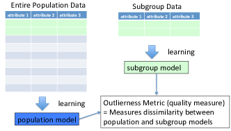
Figure 1: A general schema for Exceptional Model Mining for propositional data

The EMM framework leverages the extensive work on model learning in machine learning for exception mining: A subgroup is exceptional to the extent that a model learned from data for the subgroup deviates from a model learned for the general population. A computational method for measuring this extent is called a quality measure; we also refer to it as an outlierness metric. For a given model type, finding an appropriate quality measure for quantifying exceptionality is the main research question in EMM. The EMM framework allows us to leverage the extensive work on statistical-relational model learning for exception mining in multi-relational data. Compared to previous EMM models, the novelty of our work is as follows. 1) EMM has so far been developed only for propositional i.i.d. data, not relational data. Accordingly EMM has not been applied with SRL models. 2) In the propositional i.i.d. setting, each object is represented by a single data row, and it is meaningless to learn a model for a single object. Instead, EMM is applied to identify exceptional subgroups of objects. With relational data, each object is represented by its own dataset (egonet, interpretation), and it is meaningful to apply EMM to identify single exceptional objects. Compared to previous relational outlier detection work, our model-based approach is novel in that it neither summarizes the object data by a feature set (as in the Oddball system, see [3]) nor looks for rules that exceptional objects violate (e.g. [19]).

Contributions

Our main contributions may be summarized as follows.

1. The first EMM approach to outlier detection for structured data that is based on a probabilistic model.

2. A new outlier score based on a novel model likelihood comparison, the log-likelihood distance.

Paper Organization

We review background about Bayesian networks for relational data. Then we describe how we apply the EMM framework to multi-relational data. We introduce a novel log-likelihood distance outlier score as the quality or outlierness metric. After presenting the details of our approach, we review related work. Empirical evaluation compares model-based and aggregation-based approaches to relational outlier detection, with respect to three synthetic and three real-world problems.

II Background: Bayesian Networks for Relational Data

We adopt the Parametrized Bayes net (PBN) formalism [26] that combines Bayes nets with logical syntax for expressing relational concepts. EMM is an inclusive framework and can in principle be applied with other SRL models, such as Markov Logic networks [9]. We worked with PBNs because i) they offer the most scalable structure learning methods [33] to support our larger datasets, and ii) the PBN conditional probability parameters can be easily interpreted, which means that the resulting exceptionality metrics can be easily interpreted (see Section I below).

II-A Bayesian Networks

A Bayesian Network (BN) is a directed acyclic graph (DAG) whose nodes comprise a set of random variables [24]. Depending on context, we interchangeably refer to the nodes and variables of a BN. Fix a set of variables $\boldsymbol{V}=\{V_{1},\ldots,V_{n}\}$. The possible values of $V_{i}$ are enumerated as $\{v_{i1},\ldots,v_{ir_{i}}\}$. The notation $P(V_{i}=v)\equiv P(v)$ denotes the probability of variable $V_{i}$ taking on value $v$. We also use the vector notation $P(\boldsymbol{V}=\mathbf{v})\equiv P(\mathbf{v})$ to denote the joint probability that each variable $V_{i}$ takes on value $\mathbf{v}_{i}$.

The conditional probability parameters of a Bayesian network specify the distribution of a child node given an assignment of values to its parent node. For an assignment of values to its nodes, a BN defines the joint probability as the product of the conditional probability of the child node value given its parent values, for each child node in the network. This means that the log-joint probability can be decomposed as the node-wise sum

$$\ln P(\boldsymbol{V}=\mathbf{v};B,\boldsymbol{\theta})=\sum_{i=1}^{n}\ln\theta(\mathbf{v}_{i}|\mathbf{v}_{\mathbf{pa}_{i}})$$ (1)

where $\mathbf{v}_{i}$ resp. $\mathbf{v}_{\mathbf{pa}_{i}}$ is the assignment of values to node $V_{i}$ resp. the parents of $V_{i}$ determined by the assignment $\mathbf{v}$. To avoid difficulties with $\ln(0)$, here and below we assume that joint distributions are positive everywhere. Since the parameter values for a Bayes net define a joint distribution over its nodes, they therefore entail a marginal, or unconditional, probability for a single node. We denote the marginal probability that node $V$ has value $v$ as $P(V=v;B,\boldsymbol{\theta})\equiv\theta(v)$.

Example.

Figure 2 shows an example of a Bayesian network and associated joint and marginal probabilities.

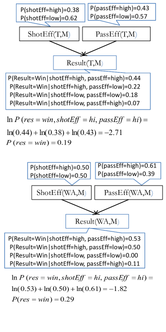
Figure 2: Example of joint and marginal probabilities computed from a toy Bayesian network structure. The parameters were estimated from the Premier League dataset. (Top): A class model Bayesian network $B_{c}$ for all teams with class parameters $\boldsymbol{\theta}_{c}$. (Bottom): The same Bayesian network structure with object parameters $\boldsymbol{\theta}_{o}$ learned for Wigan Athletics ($T=WA$). Our model-based methods outlier scores compare the data likelihood of the class parameters and the object parameters.

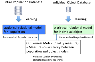
Figure 3: The EMM approach for statistical-relational models. The model class we utilize in this paper are Parametrized Bayesian networks, with a log-linear likelihood function. As outlierness metrics we consider the standard Kullback-Leibler divergence, and a novel divergence introduced in this paper.

II-B Relational Data

We adopt a functor-based notation for combining logical and statistical concepts [26, 16]. A functor is a function or predicate symbol. Each functor has a set of values (constants) called the domain of the functor. The domain of a predicate is $\{\mathit{T},\mathit{F}\}$. Predicates are usually written with uppercase Roman letters, other terms with lowercase letters. A predicate of arity at least two is a relationship functor. Relationship functors specify which objects are linked. Other functors represent features or attributes of an object or a tuple of objects (i.e., of a relationship). A population is a set of objects. A term is of the form $f(\sigma_{1},\ldots,\sigma_{k})$ where $f$ is a functor and each $\sigma_{i}$ is a first-order variable or a constant denoting an object. A term is ground if it contains no first-order variables; otherwise it is a first-order term. In the context of a statistical model, we refer to first-order terms as Parametrized Random Variables (PRVs) [16]. A grounding replaces each first-order variable in a term by a constant; the result is a ground term. A grounding may be applied simultaneously to a set of terms. A relational database $\mathcal{D}$ specifies the values of all ground terms, which can be listed in data tables.

Consider a joint assignment $P(\boldsymbol{V}=\mathbf{v})$ of values to a set of PRVs $\boldsymbol{V}$. The grounding space of the PRVs is the set of all possible grounding substitutions, each applied to all PRVs in $\boldsymbol{V}$. The count of groundings that satisfy the assignment with respect to a database $\mathcal{D}$ is denoted by $\#_{\mathcal{D}}(\boldsymbol{V}=\mathbf{v})$. The database frequency $P_{\mathcal{D}}(\boldsymbol{V}=\mathbf{v})$ is the grounding count divided by the number of all possible groundings.

Example. The Opta dataset represents information about premier league data (Sec. VI-B). The basic populations are teams, players, matches, with corresponding first-order variables $\it{T},\it{P},\it{M}$. Table II specifies values for some ground terms. The first three column headers show first-order variables ranging over different populations. The remaining columns represent features. Table III illustrates grounding counts. Counts are based on the 2011-2012 Premier League Season. We count only groundings $(\it{team},\it{match})$ such that $\it{team}$ plays in $\it{match}$. Each team, including Wigan Athletics, appears in 38 matches. The total number of team-match pairs is $38\times 20=760$.

TABLE I: Sample Population Data Table (Soccer).

MatchId M	TeamId T	PlayerId P	First_goal(P,M)	TimePlayed(P,M)	ShotEff(T,M)	result(T,M)
117	WA	McCarthy	0	90	0.53	win
148	WA	McCarthy	0	85	0.57	loss
15	MC	Silva	1	90	0.59	win
…	…	…	…	…	…

TABLE II: Sample Object Data Table, for team $\it{T}=\it{WA}$.

MatchId M	TeamId $\it{T}=\it{WA}$	PlayerId P	First_goal(P,M)	TimePlayed(P,M)	ShotEff(WA,M)	result(WA,M)
117	WA	McCarthy	0	90	0.53	win
148	WA	McCarthy	0	85	0.57	loss
…	WA	…	…	…	…

A novel aspect of our paper is that we learn model parameters for specific objects as well as for the entire population. The appropriate object data table is formed from the population data table by restricting the relevant first-order variable to the target object. For example, the object database for target Team $\it{WiganAthletic}$, forms a subtable of the data table of Table II that contains only rows where TeamID = $\it{WA}$; see Table II. In database terminology, an object database is like a view centered on the object. The object database is an individual-centered representation [11].

TABLE III: Example of Grounding Count and Frequency in Premier League Data, for the conjunction $\it{passEff(T,M)=hi},shotEff(T,M)=hi,Result(T,M)=win$.

Database	Count or $\#_{D}(\boldsymbol{V}=\mathbf{v})$	Frequency or $P_{D}(\boldsymbol{V}=\mathbf{v})$
Population	76	$76/760=0.10$
Wigan Athletics	7	$7/38=0.18$

II-C Bayesian Networks for Relational Data

A Parametrized Bayesian Network Structure (PBN) is a Bayesian network structure whose nodes are PRVs. The relationships and features in an object database define a set of nodes for Bayes net learning; see Figure 2.

II-C1 Model Likelihood for Parametrized Bayesian Networks

A standard method for applying a generative model assumes that the generative model represents normal behavior since it was learned from the entire population. An object is deemed an outlier if the model assigns sufficiently low likelihood to generating its features [6]. This likelihood method is an important baseline for our investigation. Defining a likelihood for relational data is more complicated than for i.i.d. data, because an object is characterized not only by a feature vector, but by an object database. We employ the relational pseudo log-likelihood [31], which can be computed as follows for a given Bayesian network and database.

$$\it{LOG}(\mathcal{D},B,\boldsymbol{\theta})=\sum_{i=1}^{n}\sum_{j=1}^{r_{i}}\sum_{\mathbf{pa}_{i}}P_{\mathcal{D}}(v_{ij},\mathbf{pa}_{i})\ln\theta(v_{ij}|\mathbf{pa}_{i})$$ (2)

Equation (2) represents the standard BN log-likelihood function for the object data [8], except that parent-child instantiation counts are standardized to be proportions [31]. The equation can be read as follows.

1. For each parent-child configuration, use the conditional probability of the child given the parent.

2. Multiply the logarithm of the conditional probability by the database frequency of the parent-child configuration.

3. Sum this product over all parent-child configurations and all nodes.

Schulte proves that the maximum of the pseudo-likelihood  (2) is given by the empirical database frequencies [31, Prop.3.1.]. In all our experiments we use these maximum likelihood parameter estimates.

Example. The family configuration

$$\it{passEff(T,M)=hi},shotEff(T,M)=hi,Result(T,M)=win$$

contributes one term to the pseudo log-likelihood for the BN of Figure 2. For the population database, this term is $0.1\times\ln(0.44)=-0.08$. For the Wigan Athletics database, the term is $0.18\times\ln(0.44)=-0.14$.

III EMM for Relational Data

This section describes our approach to applying the EMM framework to relational data, using the following notation.

• $\mathcal{D}_{C}$ is the database for the entire class of objects; cf. Table II. This database defines the class distribution $P_{C}\equiv P_{\mathcal{D}_{c}}$.

• $\mathcal{D}_{o}$ is the restriction of the input database to the target object; cf. Table II. This database defines the object distribution $P_{o}\equiv P_{\mathcal{D}_{o}}$.

• $B_{C}$ is a model (e.g., Bayesian network) learned with $\mathcal{D}_{\mathcal{P}}$ as the input database; cf. Figure 2(a).

• $\boldsymbol{\theta}_{C}$ resp. $\boldsymbol{\theta}_{o}$ are parameters learned for $B_{C}$ using $\mathcal{D}_{c}$ resp. $\mathcal{D}_{o}$ as the input database.

Figure 3 illustrates these concepts and the system flow for computing an outlierness score. First, we learn a Bayesian network $B_{C}$ for the entire population using a previous learning algorithm (see Section VI-C below). We then evaluate how well the class model fits the target object data. For vectorial data, the standard model fit metric is the log-likelihood of the target datapoint. For relational data, the counterpart is the relational log-likelihood (2) of the target database:

$$\it{LOG}(\mathcal{D}_{o},B_{C},\boldsymbol{\theta}_{C}).$$ (3)

While this is a good baseline outlier score, it can be improved by considering scores based on the likelihood ratio, or log-likelihood difference:

$$\it{LR}(\mathcal{D}_{o},B_{C},\boldsymbol{\theta}_{o})\equiv\it{LOG}(\mathcal{D}_{o},B_{C},\boldsymbol{\theta}_{o})-\it{LOG}(\mathcal{D}_{o},B_{C},\boldsymbol{\theta}_{C}).$$ (4)

The log-likelihood difference compares how well the class-level parameters fit the object data, vs. how well the object parameters fit the object data. In terms of the conditional probability parameters, it measures how much the log-conditional probabilities in the class distribution differ from those in the object distribution. Note that this definition applies only for relational data where an individual is characterized by a substructure rather than a “flat” feature vector. Assuming maximum likelihood parameter estimation, $\it{LR}$ is equivalent to the Kullback-Leibler divergence between the class-level and object-level parameters [8]. While the $\it{LR}$ score provides more outlier information than the model log-likelihood, it can be improved further by two transformations as follows. (1) Decompose the joint probability into a single-feature component and a mutual information component. (2) Replace log-likelihood differences by log-likelihood distances. The resulting score is the log-likelihood distance ($\it{ELD}$), which is the main novel score we propose in this paper. Formally it is defined as follows for each feature $i$. The total score is the sum of feature-wise scores. Section IV below provides example computations.

$$\begin{array}[]{l}\it{ELD}_{i}=\sum_{j=1}^{r_{i}}P_{o}(v_{ij})\left|\ln\frac{\theta_{o}(v_{ij})}{\theta_{C}(v_{ij})}\right|+\\ \sum_{j=1}^{r_{i}}\sum_{\mathbf{pa}_{i}}P_{o}(v_{ij},\mathbf{pa}_{i})\left|\ln\frac{\theta_{o}(v_{ij}|\mathbf{pa}_{i})}{\theta_{o}(v_{ij})}-\ln\frac{\theta_{C}(v_{ij}|\mathbf{pa}_{i})}{\theta_{C}(v_{ij})}\right|.\end{array}$$ (5)

The first sum is the single-feature component, where each feature is considered independently of all others. It computes the expected log-distance with respect to the singe feature value probabilities between the object and the class models. The second $\it{ELD}$ sum is the mutual information component, based on the mutual information among all features. It computes the expected log-distance between the object and the class models with respect to the mutual information of feature value assignments. Intuitively, the first sum measures how the models differ if we treat each feature in isolation. The second sum measures how the models differ in terms of how strongly parent and child features are associated with each other.

III-A Motivation

The motivation for the mutual information decomposition is two-fold.

(1) Interpretability, which is very important for outlier detection. The single-feature components are easy to interpret since they involve no feature interactions. Each parent-child local factor is based on the average relevance of parent values for predicting the value of the child node, where relevance is measured by $\ln(\theta(v_{ij}|\mathbf{pa}_{i})/\theta(v_{ij}))$. This relevance term is basically the same as the widely used lift measure [35], therefore an intuitively meaningful quantity. The $\it{ELD}$ score compares how relevant a given parent condition is in the object data with how relevant it is in the general class.

(2) Avoiding cancellations. Each term in the log-likelihood difference (4) decomposes into a relevance difference and a marginal difference:

$$\ln\frac{\theta_{o}(v_{ij}|\mathbf{pa}_{i})}{\theta_{C}(v_{ij}|\mathbf{pa}_{i})}=\ln\frac{\theta_{o}(v_{ij}|\mathbf{pa}_{i})}{\theta_{o}(v_{ij})}-\ln\frac{\theta_{C}(v_{ij}|\mathbf{pa}_{i})}{\theta_{C}(v_{ij})}+\ln\frac{\theta_{o}(v_{ij})}{\theta_{C}(v_{ij})}.$$ (6)

These differences can have different signs for different child-parent configurations and cancel each other out; see Table IV. Taking distances as in Equation 5 avoids this undesirable cancellation. Since our goal is to assess the distinctness of an object, we do not want differences to cancel out. The general point is that averaging differences is appropriate when considering costs, or utilities, but not appropriate for assessing the distinctness of an object. For instance, the average of both vectors (0,0) and (1,-1) is 0, but their distance is not.

III-B Comparison Outlier Scores

Our lesion study compares our log-likelihood distance $\it{ELD}$ score to baselines that are defined by omitting a component of $\it{ELD}$. In this section we define these scores. The scores increase in sophistication in the sense that they apply more transformations of the log-likelihood ratio. More sophisticated scores provide more information about outliers. Table IV defines local feature scores; the total score is the sum of feature-wise scores. All metrics are defined such that a higher score indicates a greater anomaly. The metrics are as follows.

is the first component of the $\it{ELD}$ score. It considers each feature independently (no feature correlations).

is the standard model-based outlier detection score using data likelihood.

is the log-likelihood difference (4) between the class-level and object-level parameters.

replaces differences in $\it{LR}$ by distances.

applies a mutual information decomposition to $\it{LR}$.

TABLE IV: Baseline Outlier Scores for Bayesian Networks

Method	Formula
$\it{FD}_{i}$	$\begin{array}[]{l}\sum_{i=1}^{n}\sum_{j=1}^{r_{i}}P_{o}(v_{ij})\left|\ln\frac{\theta_{o}(v_{ij})}{\theta_{C}(v_{ij})}\right|\end{array}$
$-\it{LOG}_{i}$	$\begin{array}[]{l}-\sum_{i=1}^{n}\sum_{j=1}^{r_{i}}\sum_{\mathbf{pa}_{i}}P_{o}(v_{ij},\mathbf{pa}_{i})\ln\theta_{C}(v_{ij}|\mathbf{pa}_{i})\end{array}$
$\it{LR}_{i}$	$\begin{array}[]{l}\sum_{j=1}^{r_{i}}\sum_{\mathbf{pa}_{i}}P_{o}(v_{ij},\mathbf{pa}_{i})\ln\frac{\theta_{o}(v_{ij}|\mathbf{pa}_{i})}{\theta_{C}(v_{ij}|\mathbf{pa}_{i})}.\end{array}$
$|\it{LR}_{i}|$	$\begin{array}[]{l}\sum_{j=1}^{r_{i}}\sum_{\mathbf{pa}_{i}}P_{o}(v_{ij},\mathbf{pa}_{i})|\ln\frac{\theta_{o}(v_{ij}|\mathbf{pa}_{i})}{\theta_{C}(v_{ij}|\mathbf{pa}_{i})}|.\end{array}$
$\it{LR}_{i}^{+}$	$\begin{array}[]{l}\sum_{j=1}^{r_{i}}P_{o}(v_{ij})\ln\frac{\theta_{o}(v_{ij})}{\theta_{C}(v_{ij})}+\\ \sum_{j=1}^{r_{i}}\sum_{\mathbf{pa}_{i}}P_{o}(v_{ij},\mathbf{pa}_{i})\ln\frac{\theta_{o}(v_{ij}|\mathbf{pa}_{i})}{\theta_{o}(v_{ij})}-\ln\frac{\theta_{C}(v_{ij}|\mathbf{pa}_{i})}{\theta_{C}(v_{ij})}.\end{array}$

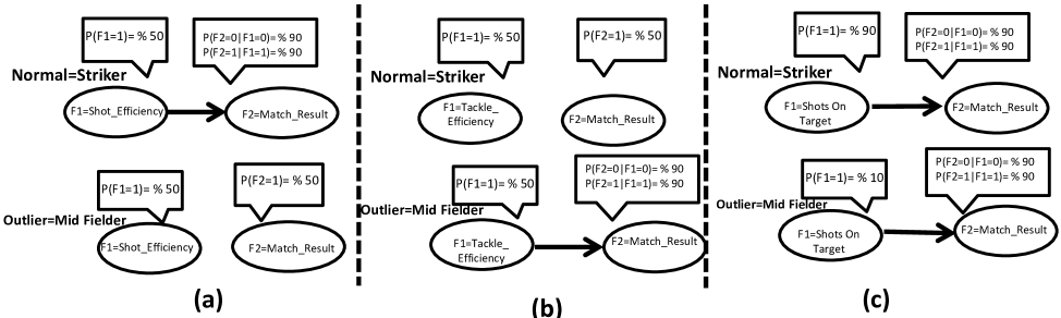
Figure 4: Illustrative Bayesian networks. The networks are not learned from data, but hand-constructed to be plausible for the soccer domain. (a) High Correlation: Normal individuals exhibit a strong association between their features, outliers no association. Both normals and outliers have a close to uniform distribution over single features. (b) Low Correlation: Normal individuals exhibit no association between their features, outliers have a strong association. Both normals and outliers have a close to uniform distribution over single features. (c) Single Attributes: Both normal and outlier individuals exhibit a strong association between their features. In normals, 90% of the time, feature 1 has value 0. For outliers, feature 1 has value 0 only 10% of the time.

IV Examples

We provide three simple examples with only two features that illustrate the computation of the outlier scores. They are designed so that outliers and normal objects are easy to distinguish, and so that it is easy to trace the behavior of an outlier score. The examples therefore serve as thought experiments that bring out the strengths and weaknesses of model-based outlier scores. Figure 4 describes the BN representation of the examples. Table V provides the computation of the scores. For intuition, we can think of a soccer setting, where each match assigns a value to each attribute $F_{i},i=1,2$ for each player. Scores for the $F_{2}$ feature are computed conditional on $F_{1}=1$. Expectation terms are computed first for $F_{2}=1$, then $F_{2}=0$.

The single feature distributions are uniform, so the feature component $\it{ELD}_{1}$ is 0 for each node in both examples. The table illustrates the undesirable cancelling effects in $\it{LR}$. In the high correlation scenario 4(a), the outlier object has a lower probability than the normal class distribution of $\it{Match\_Result}=0$ given that $\it{Shot\_Efficiency}=1$. Specifically, 0.5 vs. 0.9. The outlier object exhibits a higher probability $\it{Match\_Result}=1$ than the normal class distribution, conditional on $\it{Shot\_Efficiency}=1$; specifically, 0.5 vs. 0.1. In line 1, column 2 of Table V the log-ratios $\ln(0.5/0.9)$ and $\ln(0.5/0.1)$ therefore have different signs. In the low correlation scenario 4(b), the cancelling occurs in the same way, but with the normal and outlier probabilities reversed. The cancelling effect is even stronger for attributes with more than two possible values.

TABLE V: Example Computation of different outlier scores.

Score	$F1=1$ Computation	$F2|F1=1$ Computation	Result
$\it{LR}$	$1/2\ln(0.5/0.5)=0$	$1/4\ln(0.5/0.9)+1/4\ln(0.5/0.1)$	0.36
$|\it{LR}|$	$0$ (no parents)	$1/4|\ln(0.5/0.5)-\ln(0.9/0.5)|+1/4|\ln(0.5/0.5)-\ln(0.1/0.5)|$	0.79
$\it{FD}$	$|\ln(0.5/0.5)|=0$	$1/2|\ln(0.5/0.5)|+1/2|\ln(0.5/0.5)|$	0
ELD	$0+0$	$0.79+\it{FD}$	0.79

Table V(a): High Correlation Case, Figure 4(a).

Score	$F1=1$ Computation	$F2|F1=1$ Computation	Result
$\it{LR}$	$1/2\ln(0.5/0.5)=0$	$0.5\cdot 0.9\ln(0.9/0.5)+0.5\cdot 0.1\ln(0.1/0.5)$	0.26
$|\it{LR}|$	$0$ (no parents)	$0.5\cdot 0.9|\ln(0.9/0.5)-\ln(0.5/0.5)|+0.5\cdot 0.1|\ln(0.1/0.5)-\ln(0.5/0.5)|$	0.50
$\it{FD}$	$|\ln(0.5/0.5)|=0$	$1/2|\ln(0.5/0.5)|+1/2|\ln(0.5/0.5)|$	0
$\it{ELD}$	$0+0$	$0.5+\it{FD}$	0.5

Table V(b): Low Correlation Case. Figure 4(b).

V Related Work

Outlier detection is a densely researched field, for a survey please see [2]. Figure 5 provides a tree picture of where our method is situated with respect to other outlier detection methods and other data models. Our method falls in the category of unsupervised statistical model-based approaches. To our knowledge, ours is the first model-based method tailored for object-relational data. Like other model-based approaches, it detects global outliers. Aggarwal [2] defines a global outlier to be a data point that notably deviates from the rest of the population. We review relevant approaches from different data models, the most common atomic object model—where data is represented by vectors—and structured data models. Akoglu et al. provide an excellent recent survey of outlier detection in relational models [3].

a) Attribute Vector Data Model: By far most work on outlier detection considers atomic objects with flat feature vectors. This leads to an impedance mismatch: The required input format for these outlier detection methods is a single data matrix, not a structured dataset. For example, one cannot provide a relational database as input. This mismatch is not simply a question of choosing a file format, but instead reflects a different underlying data model: complex objects with both attributes and component objects vs. atomic objects with attributes only. It is possible to “flatten” structured data by converting it to unstructured feature vectors, for instance by using aggregate functions. We evaluated the aggregation approach in this paper by applying three standard methods for outlier detection.

Work on atomic contextual outliers [34] is like ours in that it considers the distinctness of a target individual from a reference class. A reference class is not specified for each object, but is constructed as part of outlier detection. Our work could be combined with a class discovery approach by providing a score of how informative the inferred classes are.

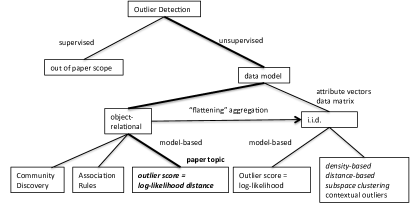
Figure 5: A tree structure for related work on outlier detection for structured data. A path specifies an outlier detection problem, the leaves list major approaches to the problem. Approaches in italics appear in experiments.

b) Structured Data Models: We discuss related techniques in three types of structured data models: SQL (relational), XML (hierarchical), and OLAP (multi-dimensional).

For relational data, many outlier detection approaches aim to discover rules that represent the presence of anomalous associations for an individual or the absence of normal associations [19, 12]. The survey by [23] unifies within a general rule search framework related tasks such as exception mining, which looks for associations that characterize unusual cases, subgroup mining, which looks for associations characterizing important subgroups, and contrast space mining, which looks for differences between classes. Another rule-based approach uses Inductive Logic Programming techniques [4]. While local rules are informative, they are not based on a global statistical model and do not provide a single outlier score for each individual.

A latent variable approach in information networks ranks potential outliers in reference to the latent communities inferred by network analysis [12]. Our model aggregates information from entities and links of different types, but does not assume that different communities have been identified.

Koh et al. [17] propose a method for hierarchical structures represented in XML document trees. Their aim is to identify feature outliers, not class outliers as in our work. Also, they use aggregate functions to convert the object hierarchy into feature vectors. Their outlier score is based on local correlations, and they do not construct a model.

The multi-dimensional data model defines numeric measures for a set of dimensions. The differences in the two data models mean that multi-dimensional outlier detection models [30] do not carry over to object-relational outlier detection. (1) The object data model allows but does not require any numeric measures. In our datasets, all features are discrete. Nor do we assume that it is possible to aggregate numeric measures to summarize lower-level data at higher levels. (2) In scoring a potential outlier object, our method considers other objects both below and above the target object in the component hierarchy. OLAP exploration methods consider only cells below or at the same level as the target cell. For example, in scoring a player, our method would consider features of the player’s team. Also, the $\it{ELD}$ outlier score of an object is not determined by the outlier scores of its components, in contrast to the approach of Sarawagi et al.. (3) Our approach models a joint distribution over features, exploiting correlations among features. Most of the OLAP-based methods consider only a single numeric measure at a time, not a joint model.

Statistical data cleaning methods are related to outlier detection, in that erroneous data may be detected as outliers (e.g., [7]). Nonetheless, these data cleaning methods differ from our work in several ways. 1) Although they often originate in the database community, they are usually developed only for single-table propositional data, not relational data. (An exception is the ERACER system [20].) 2) Our work assumes that the data is (mainly) correct, and identifies exceptional identities for the given data. 3) Data cleaning methods focus on unusual values or tuples (e.g. a mistaken rating for a movie by a user), not exceptional subdatabases or egonets.

VI Experimental Design

All the experiments were performed on a 64-bit Centos machine with 4GB RAM and an Intel Core i5-480 M processor. The likelihood-based outlier scores were computed with SQL queries using JDBC, JRE 1.7.0. and MySQL Server version 5.5.34. We describe the datasets used in our experiments.

VI-A Synthetic Datasets

We generated three synthetic datasets with normal and outlier players using the distributions represented in the three Bayesian networks of Figure 4. Each player participates in 38 matches, similar to the real-world data. The main goal of designing synthetic experiments is to test the methods on easy to detect outliers. Each match assigns a value to each feature $F_{i},i=1,2$ for each player.

High Correlation See Figure 4(a).

Low Correlation See Figure 4(b).

Single features See Figure 4(c).

We used the $\it{mlbench}$ package in $\it{R}$ to generate synthetic features in matches, following these distributions for 240 normal players and 40 outliers. We followed the real-world Opta data in terms of number of normal and outlier individuals. The scores are used to rank all 280 players.

VI-B Real-World Datasets

Data tables are prepared from Opta data [21] and IMDb [14]. Our datasets and code are available on-line [15].

Soccer Data

The Opta data were released by Manchester City. It lists box scores, that is, counts of all the ball actions within each game by each player, for the 2011-2012 season. For each player in a match, our data set contains eleven player features. For each team in a match, there are five features computed as player feature aggregates, as well as the team formation and the result (win, tie, loss). There are two relationships, $\it{Appears\_Player}(P,M)$, $\it{Appears\_Team}(T,M)$.

IMDB Data

The Internet Movie Database (IMDB) is an on-line database of information related to films, television programs, and video games. The IMDB website offers a dataset containing information on cast, crew, titles, technical details and biographies into a set of compressed text files. We preprocessed the data like [25] to obtain a database with seven tables: one for each population and one for the three relationships $\it{Rated}(\it{User},\it{Movie})$, $\it{Directs}(\it{Director},\it{Movie})$, and $\it{ActsIn}(\mathit{Actor},\it{Movie})$.

In real-world data, there is no ground truth about which objects are outliers. To address this issue, we employ a one-class design: we learn a model for the class distribution, with data from that class only. Then we rank all individuals from the normal class together with all objects from a contrast class treated as outliers, to test whether an outlier score recognizes objects from the contrast class as outliers. Table VI shows the normal and contrast classes for three different datasets. In-class outliers are possible, e.g. unusual strikers are still members of the striker class. Our case studies describe a few in-class outliers. In the soccer data, we considered only individuals who played more than 5 matches out of a maximum 38.

TABLE VI: Outlier/normal Objects in Real-World Datasets.

Normal	#Normal	Outlier	#Outlier
Striker	153	Goalie	22
Midfielder	155	Striker	74
Drama	197	Comedy	47

VI-C Methods Compared

We compare two types of approaches, and within each approach several outlier detection methods. The first approach evaluates the likelihood-based outlier scores described in Section III. For relational Bayesian network structure learning we utilize the previous learn-and-join algorithm (LAJ), which is a state-of-the-art BN structure learning method for relational data [32]. The LAJ algorithm employs an iterative deepening strategy, which can be described as as search through a lattice of table joins. For each table join, different BNs are learned and the learned edges are propagated from smaller to larger table joins. For a full description, complexity analysis, and learning time measurements, please see [32]. We used the implementation of the LAJ algorithm due to its creators [15].

The second approach first “flattens” the structured data into a matrix of feature vectors, then applies standard matrix-based outlier detection methods. We refer to such methods as aggregation-based (cf. Figures 5). For example, this was the approach taken by Breunig et al. for identifying anomalous players in sports data [5]. Following their paper, for each continuous feature in the object data, we use the average over its values, and for each discrete feature, we use the occurrence count of each feature value in the object data. Aggregation tends to lose information about correlations. Our experiments address the empirical question of whether this loss of information affects outlier detection. We evaluated three standard matrix-based outlier detection methods: Density-based $\it{LOF}$ [5], distance-based $\it{KNNOutlier}$ [27] and subspace analysis $\it{OutRank}$ [22]. These represent common, fundamental approaches for vectorial data. Like $\it{ELD}$, subspace analysis is sensitive to correlations among features. We used the available implementation of all three data matrix methods from the state of the art data mining software ELKI [1]. We used PRO-CLUS as the clustering function for $\it{OutRank}$, recommended by [22].

VII Empirical Results

We present results regarding computational feasibility, predictive performance, and case studies.

VII-1 Computational Cost of the $\it{ELD}$ Score.

Table VIII shows that the computation of the $\it{ELD}$ value for a given target object is feasible. On average, it takes a quarter of a minute for each soccer player, and one minute for each movie. This includes the time for parameter learning from the object database. Learning the class model BN takes longer, but needs to be done only once for the entire object class. The BN model provides a crucial low-dimensional representation of the distribution information in the data. Table VIII compares the number of terms required to compute the $\it{ELD}$ score in the BN representation to the number of terms in an unfactored representation with one parameter for each joint probability.

TABLE VII: Time (min) for computing the $\it{ELD}$ score.

Dataset	Class Model	Average per Object
Strikers vs. Goalies	4.14	0.25
Midfielder vs. Goalies	4.02	0.25
Drama vs. Comedy	8.30	1.00

TABLE VIII: The Bayesian network representation decreases the number of terms required for computing the $\it{ELD}$ score.

Dataset	#Terms Using BN	#Terms without Using BN
Strikers vs. Goalies	1,430	114,633,792
Midfielders vs. Goalies	1,376	43,670,016
Drama vs. Comedy	50,802	215,040,000

VII-2 Detection Accuracy

We follow the evaluation design of [12] and make each baseline methods detect the same percentage of objects as outliers: Sort the outlier scores obtained by the three baseline methods in descending order, and take the top $r$ percent as outliers. Then we use precision, a.k.a. true positive rate as the evaluation metric which is the percentage of correct ones in the set of outliers identified by the algorithm. As in [12], we set the percentages of outlier to be 1% and 5%. In the one-class design, precision measures how many members of the outlier class were correctly recognized. We also report some AUC measurements [2], which aggregate precision values at different percentage cutoffs.

Likelihood-Based Methods

Table IX shows the $\it{Precision}$ values for each probabilistic ranking. Our $\it{ELD}$ score achieves the top score on each dataset. On the synthetic data, $\it{ELD}$ and $|\it{LR}|$ are the only scores with 100% precision at 1% and 5%. This confirms the value of using distances rather than differences. While it ought to be easy to distinguish the outliers, Table X shows that $\it{ELD}$ is the only score that achieves perfect detection, that is AUC = 1.0.

TABLE IX: Precision of outlier scores in different datasets.

Dataset	percentage	Model-based models					Aggregation-based models
		ELD	$|\it{LR}|$	LR	FD	LOG	LOF	$\it{OutRank}$	KNNOutlier
High-Correlation	1%	1.00	1.00	0.73	0.47	0.91	0.11	0.53	0.48
	5%	1.00	1.00	0.85	0.65	0.95	0.22	0.50	0.65
Low-Correlation	1%	1.00	1.00	0.87	0.14	0.93	0.10	0.00	0.06
	5%	1.00	1.00	0.90	0.25	0.95	0.25	0.10	0.14
Single-Feature	1%	1.00	1.00	0.39	0.53	0.81	0.46	1.00	0.51
	5%	1.00	1.00	0.55	0.62	0.92	0.55	1.00	0.54
Striker-Goalie	5%	0.57	0.27	0.22	0.51	0.36	0.19	0.47	0.42
	15%	0.63	0.36	0.31	0.58	0.40	0.32	0.50	0.52
Midfielder-Striker	1%	0.49	0.42	0.25	0.41	0.46	0.29	0.44	0.16
	5%	0.52	0.48	0.39	0.44	0.50	0.38	0.48	0.35
Drama-Comedy	1%	0.44	0.38	0.39	0.15	0.22	0.29	0.07	0.014
	5%	0.47	0.45	0.44	0.40	0.28	0.36	0.17	0.20

TABLE X: AUC of $\it{ELD}$ vs. $|LR|$.

Score	High-Cor.	Low-Cor.	Single-F.	Striker	Midfielder	Drama
ELD	1.00	1.00	1.00	0.89	0.66	0.70
$|\it{LR}|$	0.95	0.95	0.89	0.61	0.64	0.65

Aggregation-Based Methods vs. ELD

Table IX shows the precision values for aggregation-based methods compared to $\it{ELD}$. Our $\it{ELD}$ score outperforms all aggregation-based methods on all datasets, except for a tie with $\it{OutRank}$(ProClus) on the relatively easy problem of distinguishing strikers from goalies. The performances of aggregation-based methods are most like that of the probabilistic score $\it{FD}$, which does not consider the correlation among the features. This finding reflects the fact that aggregation tends to lose information about correlations. The aggregation-based methods achieve their highest performance on the Strikers vs. Goalies dataset. In this dataset action count features such as ShotsOnTarget, ShotEfficiency point to strikers and the feature SavesMade points to goalies. Therefore, outliers in this dataset are easy to find by considering features in isolation.

VII-3 Case Studies

For a case study, we examine three top outliers as ranked by $\it{ELD}$, shown in Table XI. The aim of the case study is to provide a qualitative sense of the outliers indicated by the scores. Also, we illustrate how the BN representation leads to an interpretable ranking. Specifically, we employ a feature-wise decomposition of the score combined with a drill down analysis:

1. Find the node $V_{i}$ that has the highest $\it{ELD}_{i}$ divergence score for the outlier object.

2. Find the parent-child combination that contributes the most to the $\it{ELD}_{i}$ score for that node.

3. Decompose the $\it{ELD}$ score for the parent-child combination into feature and mutual information component.

We present strong associations—indicated by the $\it{ELD}$’s mutual information component—in the intuitive format of association rules.

Strikers vs. Goalies

In real-world data, a rare object may be a within-class outlier, i.e., highly anomalous even within its class. In an unsupervised setting without class labels, we do not expect an outlier score to distinguish such an in-class outlier from outliers outside the class. An example is the striker Edin Dzeko. He is a highly anomalous striker who obtains the top $\it{ELD}$ divergence score among both strikers and goalies. His $\it{ELD}$ score is highest for the Dribble Efficiency feature. The highest $\it{ELD}$ score for that feature occurs when Dribble Efficiency is low, and its parents have the following values: Shot Efficiency high, Tackle Efficiency medium. Looking at the single feature divergence, we see that Edin Dzeko is indeed an outlier in the Dribble Efficiency subspace: His dribble efficiency is low in 16% of his matches, whereas a randomly selected striker has low dribble efficiency in 50% of their matches. Thus, Edin Dzeko is an unusually good dribbler. Looking at the mutual information component of $\it{ELD}$, i.e., the parent-child correlations, for Edin Dzeko the confidence of the rule

$$\it{ShotEff}=\it{high},\it{TackleEff}=\it{medium}\rightarrow\it{DribbleEff}=\it{low}$$

is 50%, whereas in the general striker class it is $38\%$.

Midfielders vs. Strikers

For the single feature score, Robin van Persie is recognized as a clear striker because of the $\it{ShotsOnTarget}$ feature. It makes sense that strikers shoot on target more often than midfielders. Robin van Persie achieves a high number of shots on targets in $34\%$ of his matches, compared to $3\%$ for a random midfielder. The mutual information component shows that he also exhibits unusual correlations. For example, the confidence of the rule

$$\it{ShotEff}=\it{high},\it{TimePlayed}=\it{high}\rightarrow\it{ShotsOnTarget}=\it{high}$$

is 70% for van Persie, whereas for strikers overall it is 52%.

The most anomalous midfielder is Scott Sinclair. His most unusual feature is $\it{DribbleEfficiency}$: For feature divergence, he achieves a high dribble efficiency $50\%$ of the time, compared to a random midfielder with $30\%$.

Drama vs. Comedy

The top outlier rank is assigned to the within-class outlier $\it{BraveHeart}$. Its most unusual feature is $\it{ActorQuality}$: In a random drama movie, $42\%$ of actors have the highest quality level 4, whereas for $\it{BraveHeart}$ $93\%$ of actors achieve the highest quality level.

The $\it{ELD}$ score identifies the comedies $\it{BluesBrothers}$ and $\it{AustinPowers}$ as the top out-of-class outliers. In a random drama movie, $49\%$ of actors have casting position 3, whereas for $\it{AustinPowers}$ $78\%$ of actors have this casting position, and for $\it{BluesBrothers}$ $88\%$ of actors do.

TABLE XI: Case study for the top outliers returned by the log-likelihood distance score ELD

Strikers (Normal) vs. Goalies (Outlier)
PlayerName	Position	$\it{ELD}$ Rank	$\it{ELD}$ Max Node	$\it{ELD}$ Node Score	$\it{FD}$ Max feature Value	Object Probability	Class Probability
Edin Dzeko	Striker	1	DribbleEfficiency	83.84	DE=low	0.16	0.5
Paul Robinson	Goalie	2	SavesMade	49.4	SM=Medium	0.3	0.04
Michel Vorm	Goalie	3	SavesMade	85.9	SM=Medium	0.37	0.04
Midfielders (Normal) vs. Strikers (Outlier)
PlayerName	Position	$\it{ELD}$ Rank	$\it{ELD}$ Max Node	$\it{ELD}$ Node Score	$\it{FD}$ Max feature Value	Object Probability	Class Probability
Robin Van Persie	Striker	1	ShotsOnTarget	153.18	ST=high	0.34	0.03
Wayne Rooney	Striker	2	ShotsOnTarget	113.14	ST=high	0.26	0.03
Scott Sinclair	Midfielder	6	DribbleEfficiency	71.9	DE=high	0.5	0.3
Drama (Normal) vs. Comedy (Outlier)
MovieTitle	Genre	$\it{ELD}$ Rank	$\it{ELD}$ Max Node	$\it{ELD}$ Node Score	$\it{FD}$ Max feature Value	Object Probability	Class Probability
Brave Heart	Drama	1	ActorQuality	89995.4	a_quality=4	0.93	0.42
Austin Powers	Comedy	2	Cast_Position	61021.28	Cast_Num=3	0.78	0.49
Blue Brothers	Comedy	3	Cast_Position	24432.21	Cast_num=3	0.88	0.49

VIII Conclusion

We presented a new approach for applying Bayes nets to object-relational outlier detection, a challenging and practically important topic for machine learning. This approach follows the general framework of Exceptional Model Mining [10], and applies it to multi-relational data. The key idea is to learn one set of parameter values that represent class-level associations, another set to represent object-level associations, and compare how well each parametrization fits the relational data that characterize the target object. The classic metric for comparing two parametrized models is their log-likelihood ratio; we refined this concept to define a new relational log-likelihood distance metric via two transformations: (1) a mutual information decomposition, and (2) replacing log-likelihood differences by log-likelihood distances. This metric combines a single feature component, where features are treated as independent, with a correlation component that measures the deviation in the features’ mutual information.

In experiments on three synthetic and three real-world outlier sets, the log-likelihood distance achieved the best detection accuracy. The alternative of converting the structured data to a flat data matrix via aggregation had a negative impact. Case studies showed that the log-distance score leads to easily interpreted rankings.

There are several avenues for future work. (i) A limitation of our current approach is that it ranks potential outliers, but does not set a threshold for a binary identification of outlier vs. non-outlier. (ii) Our divergence uses expected L1-distance for interpretability, but other distance scores like L2 could be investigated as well. (iii) Extending the expected L1-distance for continuous features is a useful addition.

In sum, outlier metrics based on model likelihoods are a new type of structured outlier score for object-relational data. Our evaluation indicates that this model-based score provides informative, interpretable, and accurate rankings of objects as potential outliers.

References

- [1] E. Achtert, H. Kriegel, E. Schubert, and A. Zimek. Interactive data mining with 3d-parallel coordinate trees. In Proceedings of the 2013 ACM SIGMOD, New York, NY, USA, 2013.
- [2] C. Aggarwal. Outlier Analysis. Springer New York, 2013.
- [3] L. Akoglu, H. Tong, and D. Koutra. Graph based anomaly detection and description: a survey. Data Mining and Knowledge Discovery, 29(3):626–688, 2015.
- [4] F. Angiulli, G. Greco, and L. Palopoli. Outlier detection by logic programming. ACM Transactions on Computer Logic, 2004.
- [5] M. Breunig, H.-P. Kriegel, R. T. Ng, and J. Sander. Lof: Identifying density-based local outliers. In Proceedings of ACM SIGMOD, 2000.
- [6] A. Cansado and A. Soto. Unsupervised anomaly detection in large databases using Bayes Nets. Appllied Artificial Intelligence, 2008.
- [7] S. De, Y. Hu, V. V. Meduri, Y. Chen, and S. Kambhampati. Bayeswipe: A scalable probabilistic framework for improving data quality. Journal of Data and Information Quality (JDIQ), 8(1):5, 2016.
- [8] L. de Campos. A scoring function for learning Bayes nets based on mutual information and conditional independence tests. Journal of Machine learning Research, 2006.
- [9] P. Domingos and D. Lowd. Markov Logic: An Interface Layer for Artificial Intelligence. Morgan and Claypool Publishers, 2009.
- [10] W. Duivesteijn, A. J. Feelders, and A. Knobbe. Exceptional model mining. Data Mining and Knowledge Discovery, 30(1):47–98, 2016.
- [11] P. A. Flach. Knowledge representation for inductive learning. In Symbolic and Quantitative Approaches to Reasoning and Uncertainty, pages 160–167. Springer, 1999.
- [12] J. Gao, F. Liang, W. Fan, Y. Wang, and J. Han. On community outliers and their detection in information network. In Proceedings of ACM SIGKDD, 2010.
- [13] L. Getoor and B. Taskar. Introduction to statistical relational learning. MIT Press, 2007.
- [14] Internet Movie Database. Internet movie database. [Online]. Available: URL = http://www.imdb.com/.
- [15] H. Khosravi, T. Man, J. Hu, E. Gao, and O. Schulte. Learn and join algorithm code. [Online]. Available: URL = http://www.cs.sfu.ca/~oschulte/jbn/.
- [16] A. Kimmig, L. Mihalkova, and L. Getoor. Lifted graphical models: a survey. Computing Research Repository, 2014.
- [17] J. L. Koh, M. L. Lee, W. Hsu, and W. T. Ang. Correlation-based attribute outlier detection in XML. In Proceedings of ICDE. IEEE 24th, 2008.
- [18] D. Koller and A. Pfeffer. Object-oriented Bayes nets. In Proceedings of UAI, 1997.
- [19] J. Maervoet, C. Vens, G. Vanden Berghe, H. Blockeel, and P. De Causmaecker. Outlier detection in relational data: A case study. Expert System Applications, 2012.
- [20] C. Mayfield, J. Neville, and S. Prabhakar. Eracer: a database approach for statistical inference and data cleaning. In Proceedings of the 2010 ACM SIGMOD International Conference on Management of data, pages 75–86. ACM, 2010.
- [21] MCFC Analytics. The premier league dataset. [Online]. Available: URL = http://www.mcfc.co.uk/Home/MCFCAnalytics.
- [22] E. Muller, I. Assent, P. Iglesias, Y. Mulle, and K. Bohm. Outlier ranking via subspace analysis in multiple views of the data. In Proceedings of ICDM, 2012.
- [23] P. K. Novak, G. I. Webb, and S. Wrobel. Supervised descriptive rule discovery: A unifying survey of contrast set, emerging pattern and subgroup mining. Journal of Machine Learning Research, 2009.
- [24] J. Pearl. Probabilistic Reasoning in Intelligent Systems. Morgan Kaufmann, 1988.
- [25] V. Peralta. Extraction and Integration of MovieLens and IMDb. Technical report, APDM project, 2007.
- [26] D. Poole. First-order probabilistic inference. In Proceedings of IJCAI, 2003.
- [27] S. Ramaswamy, R. Rastogi, and K. Shim. Efficient algorithms for mining outliers from large data sets. SIGMOD, 2000.
- [28] F. Riahi and O. Schulte. Codes and Datasets. [Online]. Available:. ftp://ftp.fas.sfu.ca/pub/cs/oschulte/CodesAndDatasets/, 2015.
- [29] F. Riahi and O. Schulte. Model-based outlier detection for object-relational data. In 2015 IEEE Symposium Series on Computational Intelligence, pages 1590–1598. IEEE, 2015.
- [30] S. Sarawagi, R. Agrawal, and N. Megiddo. Discovery-driven exploration of OLAP data cubes. In Proceedings of International Conference on Extending Database Technology. Springer-Verlag, 1998.
- [31] O. Schulte. A tractable pseudo-likelihood function for Bayes nets applied to relational data. In Proceedings of SIAM SDM, 2011.
- [32] O. Schulte and H. Khosravi. Learning graphical models for relational data via lattice search. Journal of Machine Learning, 2012.
- [33] O. Schulte, H. Khosravi, and T. Man. Learning directed relational models with recursive dependencies. Machine Learning, 89:299–316, 2012.
- [34] G. Tang, J. Bailey, J. Pei, and G. Dong. Mining multidimensional contextual outliers from categorical relational data. In Proceedings of SSDBM, 2013.
- [35] S. Tuffery. Data Mining and Statistics for Decision Making. Wiley Series in Computational Statistics, 2011.