Interplay between interlayer exchange and stacking in CrI₃ bilayers

Abstract

We address the interplay between stacking and interlayer exchange for ferromagnetically ordered CrI₃, both for bilayers and bulk. Whereas bulk CrI₃ is ferromagnetic, both magneto-optical and transport experiments show that interlayer exchange for CrI₃ bilayers is antiferromagnetic. Bulk CrI₃ is known to assume two crystal structures, rhombohedral and monoclinic, that differ mostly in the stacking between monolayers. Below 210-220 Kelvin, bulk CrI₃ orders in a rhombohedral phase. Our density functional theory calculations show a very strong dependence of interlayer exchange and stacking. Specifically, the ground states of both bulk and free-standing CrI₃ bilayers are ferromagnetic for the rhombohedral phase. In contrast, the energy difference between both configurations is more than one order of magnitude smaller for the monoclinic phase, and eventually becomes antiferromagnetic when either positive strain or on-site Hubbard interactions ($U\geq 3$) are considered. We also explore the interplay between interlayer hybrydization and stacking, using a Wannier basis, and between interlayer hybrydization and relative magnetic alignment for CrI₃ bilayers, that helps to account for the very large tunnel magnetoresistance obvserved in recent experiments.

I Introduction

The recent discovery of several 2D ferromagnetic materials Gong et al. (2017); Huang et al. (2017); McGuire (2017); Fei et al. (2018); O’Hara et al. (2018) is expanding the research horizons in 2D Materials. These new materials, and more specifically CrI₃, open new venues for the fabrication of low dimensional spintronicSong et al. (2018); Klein et al. (2018); Wang et al. (2018) and optoelectronicSeyler et al. (2018); Zhong et al. (2017); Huang et al. (2018); Jiang et al. (2018a, b) devices based on multi-layer structures, and are being the object of strong interest Lado and Fernández-Rossier (2017); Liu et al. (2018a); Liu and Petrovic (2018); Richter et al. (2018); Zhang et al. (2018); Zollner et al. (2018); Jiang et al. (2018c); Liu et al. (2018b); Cardoso et al. (2018); Tong et al. (2018). Importantly, some of these applications rely on the antiparallel interlayer alignment at zero field, which can be reverted by the application of a magnetic field Song et al. (2018); Klein et al. (2018); Wang et al. (2018) or, intriguingly, electricHuang et al. (2018); Jiang et al. (2018a, b) fields.

The family of CrX₃ (X = Cl, Br, I) magnetic insulators is representative of this type of 2D ferromagnetic materials. In the single layer limit, magnetic order is very sensitive to magnetic anisotropy, that is governed by anisotropic superexchange in the case of CrI₃.Lado and Fernández-Rossier (2017); Lee et al. (2019); Besbes et al. (2019); Xu et al. (2018) Experiments in bulk show that CrCl₃ is the only one showing an anti-ferromagnetic (AF) orderMorosin and Narath (1964), while CrBr₃ and CrI₃ are bulk ferromagnetsHandy and Gregory (1952); McGuire et al. (2015) with Curie temperatures $T_{c}=37$ and $61$ K, respectively. In contrast with bulk, interlayer coupling for few layer CrI₃ is found to be antiferromagnetic, based on opticalHuang et al. (2017, 2018); Jiang et al. (2018a, b), transport Klein et al. (2018); Wang et al. (2018); Song et al. (2018); Klein et al. (2019) and, more recently, microscopic probes.Thiel et al. (2019) This provides a first motivation for this work.

The second motivation arises from the following observation. Bulk CrI₃ undergoes a structural transitionMcGuire et al. (2015) at 210-220 Kelvin, between a rhombohedral phase at low temperature and monoclinic phase at higher temperature. The layer stacking in these structures is shown in Figure 1(a,b). Interestingly, the differential magnetic susceptibility, $\frac{d\chi}{dT}$, presents a kink at the structural transitionMcGuire et al. (2015), which is consistent with a variation of the interlayer exchange interaction.

In monolayer CrI₃, the intralayer FM coupling, that ultimately drives the long-range ordering between Cr atoms, can be anticipated by the Goodenough-Kanamori rulesGoodenough (1955, 1958); Kanamori (1959) of single-ligand superexchange (M-L-M), on account of the almost perpendicular alignment between the Cr-I-Cr bonds. The extension of these rules for more than one ligand, in order to predict the interlayer exchange coupling in van der Waals structures (M-L—L-M), is not straightforward.Feldkemper and Weber (1998) In the following, we assume a different approach aiming to address the interplay between stacking and interlayer exchange coupling for CrI₃ bilayer, combining density functional theory and an effective interlayer coupling model.

II Methodology

Our calculations are based on density functional theory. For each CrI₃ stacking shown in Fig.1(a), we first perform a geometry relaxation starting from previously reported experimental crystal structure ($a=b=6.867$ Å  for the rhombohedral structure and $6.866$ Å  for the monoclinic one).McGuire et al. (2015) The relaxation is carried out using the plane-wave based code PWscf as implemented in the Quantum-Espresso ab-initio packageGiannozzi et al. (2009). For the self consistent calculations, we use a $8\times 8\times 1$ $k$-point grid for the bilayer calculations and a $12\times 12\times 6$ k-mesh for the bulk. Projector augmented wave (PAW) pseudopotentials and the Perdew-Burke-Ernzerhoff (PBE) approximationPerdew et al. (1996) for the exchange-correlation functional are used for Cr and I atoms. Van der Waals interactions are included through the Grimme-D2 model.Grimme (2006) Spin-orbit coupling is not considered in these calculations.

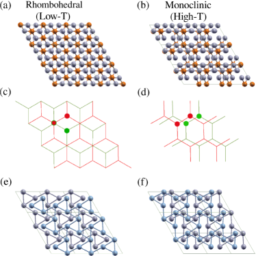
Figure 1: (Color online) Atomic structure of bilayer CrI₃ with (a) rhombohedral and (b) monoclinic crystal structure. These structures are found in bulk CrI₃ at low and high temperature. Orange and gray atoms correspond to Cr and I, respectively. (c) and (d) show the AB and AA_1/3 stacking of the hexagonal Cr lattices between the layers. The green and red lines correspond to the top and bottom hexagonal Cr lattices respectively. The green and red dots denote the Cr atoms in the top and bottom layers in the elementary unit cell. (e) Detail of the atomic structure of the I atoms at the bilayer interface for the rhombohedral stacking. (f) Idem for the monoclinic one.

III Interlayer exchange and stacking

Figures 1(c) and 1(d) show the two Cr hexagonal lattices (in red and green) and the stacking details of the bilayer. In the rhombohedral case, the two Cr lattices follows an AB or Bernal stacking, similar to bilayer graphene. The monoclinic case can be obtained by starting with an AA stacking and displacing the top layer $a$/3 along one of the in-plane lattice vectors $\vec{a}$ or $\vec{b}$ (we have labeled this stacking as AA_1/3). The two atomic structures induce a different arrangement of the I atoms at the interface which is shown in Figure 1(e,f). The position of the I atoms has an important effect on the interlayer coupling since it affects the Cr-Cr interlayer distance through steric effects (see Table 1).

We have performed first-principles calculations of bilayer (bulk) CrI₃ using both structures, namely AB (rhombohedral) and AA_1/3 (monoclinic), with different interlayer magnetic order (FM vs AF). Our results are summarized in table (1). We find that, for both bilayer and bulk CrI₃ the energy difference between the FM and AF configurations is dramatically reduced in the case of monoclinic stacking. As we discuss in section V, two different perturbations lead to an antiferromagnetic interlayer interaction for the $AA_{1/3}$ stacking of the bilayer: addition of a Hubbard $U$ correction, keeping the same geometry obtained without U, and modification of the interlayer distance.

Table 1: Summary of the calculations for bilayer (AA_1/3 vs AB) and bulk (Monoclinic vs Rhombohedral) CrI₃. The equilibrium interlayer distance ($d_{in}^{\rm PW}$) is obtained by relaxing the geometry starting from the experimental crystal structureMcGuire et al. (2015). We keep the same geometry for the two functionals, namely PBE-D2 and PBE+U-D2. D2 stands for the Grimme-D2 van der Waals correctionGrimme (2006). The energy difference is defined as $\Delta E=E_{AF}-E_{FM}$. The values of the exchange interlayer coupling are obtained from Equations 5 and 7 for bilayer and bulk respectively. The last column shows the values of $\overline{j}_{\rm 12}/N_{\rm at}$, where $N_{\rm at}$ is the number of atoms in the unit cell.

	$d_{in}^{\rm PW}$ (Å)	$\Delta E^{\rm PW}$ (meV)	$\overline{j}_{\rm in}$ ($\mu$eV)	$\overline{j}_{\rm in}$ ($\mu$eV/u.c.)
Bilayer AA1/3 (PBE-D2)	6.621	0.21	46.7	11.7
Bilayer AB (PBE-D2)	6.602	9.43	2095.6	523.9
Bilayer AA1/3 (PBE+U-D2)	6.621	-0.36	-80.7	-20.2
Bilayer AB (PBE+U-D2)	6.602	17.82	3959.7	989.9
Bulk Monoclinic (PBE-D2)	6.621	0.44	16.3	1.4
Bulk Rhombohedral (PBE-D2)	6.602	4.50	166.7	13.9

We now discuss how to relate the DFT results to the average interlayer exchange coupling ($\overline{J}_{12}$). For that matter, we assume that the interlayer exchange can be described by a classical Heisenberg model:

$${\cal H}_{\rm inter}=-\sum_{i\in 1,j\in 2}J^{\rm inter}_{ij}\vec{S}_{i}\cdot\vec{S}_{j}$$ (1)

where $1$ and $2$ label the two CrI₃ layers and $J_{ij}$ is are the interlayer exchange interactions. The sign convention we take is such that $J_{ij}>0$ ($J_{ij}<0$) stands for ferromagnetic (antiferromagnetic) interaction. Assuming that all spins are parallel, and have a length $S$, the energy for configurations where all spins in a given layer are parallel, and collinear with those of the other layer, is $U=\mp S^{2}\overline{J}_{12}$ where

$$\overline{J}_{12}=\sum_{i\in{1},j\in{2}}J^{\rm inter}_{ij}$$ (2)

is the average interlayer coupling and the sign $-$ ($+$) corresponds to the ferromagnetic (antiferromagnetic) interlayer alignment. It is self-evident that $\overline{J}_{12}$ is an increasing function of the number of atoms in the unit cell. For CrI₃, there are two atoms per unit cell and plane.

We now break down this average exchange, and the corresponding total interlayer exchange, as a sum over the contribution coming from each unit cell , $\overline{J}_{12}=N\overline{j}_{12}$, where $N$ is the number of unit cells and $\overline{j}_{12}$ is split as the sum of intracell and intercell contributions.

$$\overline{j}_{12}=\sum_{i\in(I,1),j\in(I,2)}J^{\rm intra}_{ij}+\sum_{\in(I,1),j\in(I^{\prime},2)}J^{\rm inter}_{ij}$$ (3)

Since $J^{\rm inter}_{ij}$ decays very rapidly with distance, $\overline{j}_{12}$ converges. Therefore, in the case of the bilayer, the total energy per unit cell, that can be compared with DFT calculations, reads as an Ising model for a dimer:

$${\cal U}_{\rm in}(s_{1},s_{2})=-\overline{j}_{12}S^{2}s_{1}s_{2}$$ (4)

where $s_{1},s_{2}=\pm 1$ describe the orientation of the layer magnetization. As a result, we can relate the energy difference between the parallel and antiparallel configurations in the DFT calculations with the average interlayer exchange, through

$$\Delta E\equiv{\cal U}_{\rm in}(+,-)-{\cal U}_{\rm in}(++)=2\overline{j}_{12}S^{2}$$ (5)

We now carry out the same analysis for the case of bulk, the unit cell has 3 planes. Therefore, the effective model has to keep track of the magnetization of 6 layers:

$${\cal U}_{\rm in}(s_{1},s_{2},s_{3},s_{4},s_{5},s_{6})=-\overline{j}_{12}S^{2}\sum_{i=1,6}s_{i}s_{i+1}$$ (6)

where we assume $s_{1}=s_{7}$, to account for the periodic boundary conditions in the off-plane direction. Thus, for the bulk calculations we have:

$$\Delta E\equiv{\cal U}_{\rm in}(+-+-+-)-{\cal U}_{\rm in}(++++++)=12\overline{j}_{12}S^{2}$$ (7)

Equations (5) and (7) permit to relate our DFT calculations with the average interlayer exchange. By so doing, we find that the interlayer exchange shows always a stronger ferromagnetic character than the AB (rhombohedral) phase (see Table 1) than the AA_1/3 (monoclinic). This clearly indicates that there is a correlation between stacking geometry and the interlayer exchange. This is expected, since different stacking imply both different interlayer Cr-Cr distances and Cr-I bond angles (see figure 1), which are the structural variables that control exchange.

IV Relation with experiments

Our results for bulk are consistent with the ferromagnetic interlayer interaction observed experimentally. In addition, our results might help to understand the kink in the magnetic susceptibility observed by McGuire et al. McGuire et al. (2015) at the structural phase transition observed in bulk CrI₃ at 220 Kelvin, between a low temperature rhombohedral and a high temperature monoclinic structures. The connection can be established as follows. At high temperature, CrI₃ is paramagnetic. The susceptibility of a ferromagnet in the paramagnetic regime is described by the Curie law,

$$\chi_{CW}=\frac{S(S+1)(g\mu_{B})^{2}}{3k_{B}}\frac{1}{T-T_{CW}}$$ (8)

where $S$ is the total spin of the Cr atoms, $g$ is the g-factor, $\mu_{B}$ is the Bohr magneton, $k_{B}$ is the Boltzmann constant and $T_{CW}$ is the Curie temperature, that logically depends on both the interlayer and intralayer couplings through the relation

$$3k_{B}T_{CW}=S(S+1)\overline{J}$$ (9)

where $\overline{J}=\sum_{j}(J^{\rm inter}_{ij}+J^{\rm intra}_{ij})$ is the sum of all the exchange interactions for a given spin $i$. We are assuming here that the average magnetization of all spins is the same. The calculated variation of the interlayer coupling for the two different stackings, shown in the table, will lead to a modification of $T_{CW}$ , $\Delta T_{CW}$ at the temperature of the structural transition, that leads to an additional contribution to $\frac{d\chi}{dT}\propto\frac{\partial\chi}{\partial T_{CW}}\Delta T_{CW}$.

We now discuss the relation of our results with experimental results for CrI₃ bilayers and thin filmsHuang et al. (2017, 2018); Jiang et al. (2018a, b); Klein et al. (2018); Wang et al. (2018); Song et al. (2018); Thiel et al. (2019), showing antiferromagnetic interlayer interaction. The application of off-plane magnetic fields of $B_{c}\simeq 0.35T$ and $0.6T$ revert the interlayer magnetization in CrI₃ bilayers as recently proven by transportKlein et al. (2018) and opticalHuang et al. (2017) measurements respectively. We can estimate the interlayer exchange by equating the Zeeman energy per unit cell, $E_{Z}=4\times g\mu_{B}SB_{c}$ to $\Delta E$ in eq. (4). We thus obtain $\overline{j}_{12}=\frac{-2g}{S}\mu_{B}B_{c}\simeq-60\mu eV$ and $-103\mu eV$.

Our DFT results show that interlayer exchange is much smaller for the AA_1/3 stacking, although still weakly ferromagnetic. Other density functional calculations, appeared after a first version of our work was posted in the arXiv, show that interlayer exchange can indeed become antiferromagnetic for the AA_1/3stacking, using functionals different from GGAWang et al. (2018); Jiang et al. (2018); Sivadas et al. (2018); Jang et al. (2018); Lei et al. (2019). The common point in all DFT calculations is that interlayer exchange has a weaker ferromagnetic character for the AA_1/3 stacking than for the AB.

Our DFT calculations still predict that the AB stacking is the ground state structure for the freestanding bilayer. However, the energy difference between these two stacking configurations is $\Delta E_{\rm struct}\approx 3.25$ meV/Cr atom, much smaller than its bulk counterpart, $\Delta E_{\rm struct}\approx 8$ meV/Cr atom favouring the rombohedral crystal structure. Given that experiments are always carried out with the CrI₃ bilayers deposited on top of substrates, such as graphene and silicon oxide, it can be that these favour the AA_1/3 stacking, leading to an antiferromagnetic interaction. It is also possible that stacking energetics is different in bulk and in very thin films, on account of the different contributions coming from long-range dispersive forces in both cases. Recent experimental work Thiel et al. (2019) provides evidence that this might be indeed the case.

V Effect of interlayer distance and on-site Hubbard interaction ($U$) on Interlayer exchange

We now consider two types of perturbations that could further reduce the ferromagnetic interlayer exchange and eventually yield an antiferromagnetic coupling, namely a modification of the interlayer distance and the inclusion of an on-site Hubbard interaction ($U$) using the so called PBE+U functional, in the spirit of the LDA+U approximationAnisimov et al. (1991). The first one could be driven by the coupling to the substrate, whose effect is missing in our DFT calculations. For instance, charge transfer is predicted to occur in the graphene/CrI₃ interfaceCardoso et al. (2018), that could modify interlayer separation.

Figure 2(a) shows the energy difference $\Delta E=E_{AF}-E_{FM}$ for different interlayer distances and for both structures. For $\Delta E<0$ the interlayer exchange coupling becomes AF (horizontal dashed line). This occurs in the AA_1/3 stacking for $d-d_{0}>0.2$  Å, while the AB CrI₃ remains FM. The maximal value for the AF exchange, $j_{AF}=-38\mu eV$ is obtained for $d-d_{0}=1$  Å.

We now discuss the scaling of $\Delta E$ as we change the on-site Hubbard inderaction $U$, keeping the same geometry obtained for $U=0$. Our results are shown in figure 2(c,d), for the AA_1/3 and AB stacking respectively. We observe that, in contrast to the AB stacking, the interlayer exchange in the AA_1/3 case scales non-monotonically with $U$ and, for $U\geq 3$ it becomes AF (dashed line indicates the transition from positive to negative exchange coupling).

Interestingly, we find that the response of the system to both the structural modification and the addition of a Hubbard $U$ correction, follows the same pattern. First, none of these perturbations drive the system to the AF interlayer interaction in the case of the AB stacking. Second, both perturbations drive the interlayer interaction AF in the $AA_{1/3}$ stacking. Third, the dependence of $\Delta E$ on both interlayer distance and $U$ is non-monotonic only in the case of the $AA_{1/3}$ stacking.

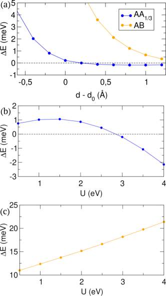
Figure 2: (Color online) (a) Energy difference $\Delta E=E_{AF}-E_{FM}$ of bilayer CrI₃ for AB (orange) and AA_1/3 (blue) stacking. $\Delta E<0$ stands for AF phase transition (horizontal dashed line). For $d-d_{0}>0.2$ Å, the AA_1/3 bilayer becomes AF. (b) Scaling of $\Delta E$ for different values of the Coulomb repulsion ($U$) in AA_1/3 stacking. For $U\geq 3$ the AA_1/3 (monoclinic) stacking becomes AF. (c) Idem for the AB (rhombohedral) stacking. In contrast to the AA_1/3 case, the AB case never becomes AF when increasin the Coulomb interaction.

Given that all known mechanisms for exchange lead to monotonic dependence with distance, the non-monotonic behaviour of $\Delta E$, for the AA_1/3 stacking, that includes a change of sign, clearly shows that interlayer exchange interaction is the result of at least two contributions with opposite signs:

$$J_{\rm in}=J^{\rm FM}_{\rm in}-J^{\rm AF}_{\rm in}.$$ (10)

The first contribution, which favours a ferromagnetic coupling, arises both from interlayer superexchange pathways and direct exchange. The second contribution favours antiferromagnetic exchange.

VI Interplay between interlayer hybridization and stacking

We now explore if interlayer antiferromagnetic exchange could be accounted for by the theory of kinetic exchange of AndersonAnderson (1963) (see also Hay et al.Hay et al. (1975)), for electrons occupying otherwise degenerate orbitals that become weakly hybridized by an interlayer hopping $\gamma$. The interlayer hopping leads to the formation of bonding-antibonding states that delocalize the states among the two layers. In the limit of on-site Hubbard repulsion $U$ much larger than $\gamma$, the low energy states of this Hubbard dimer are described by a spin Heisenberg model with antiferromagnetic exchange $J^{\rm AF}_{\rm in}=\frac{4\gamma^{2}}{\tilde{U}}$. Here, we use a Hubbard $\tilde{U}$ to differentiate it from the Hubbard $U$ used in LDA+U calculations. The former it is always present even for $U=0$ calculations, and stands for the energy that should be paid to doubly occupy an atomic orbital. The second one is the extra energy that should be paid when the orbitals are strongly localized in order to account for correlation effects.

In order to explore whether the interlayer hybdridization $\gamma$ is significantly different for the two stacking geometries for CrI₃ bilayer, we calculate the hybridization between crystal-field split $t_{2g}$. For that matter we obtain a tight-binding model from our DFT calculations, using a representation of the DFT hamiltonian in a basis of maximally localized Wannier orbitals. To do so, we use DFT as implemented in the plane-wave based PWscf code (see Methodology section), with spin-unpolarized solutions, to ensure that the band splitting comes only from the interlayer hybridization. In the non-magnetic solutions, the $t_{2g}$ bands are half filled, in contrast to the spin-polarized case, where the 3 electrons with same spin fill the 3 $t_{2g}$ bands in one spin channel. The spin-unpolarized $t_{2g}$ bands of bilayer CrI₃ for AA_1/3 and AB cases are shown in Figure 3(a,b).

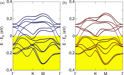
Figure 3: (Color online) Spin unpolarized band structures of bilayer CrI₃ for (a) AA_1/3 and (b) AB stacking configurations. The half-filled bands correspond to the $t_{2g}$ bands of Cr. The red and blue lines on top of the $t_{2g}$ bands corresponds to the Wannier bands.

In order to obtain a representation of the Hamiltonian in a basis of atomic-like orbitals, we transform our plane-wave basis into a localized Wannier one using wannier90 codeMostofi et al. (2014). The representation of the Hamiltonian in that basis allows us to extract the interlayer hopping amplitudes $\Gamma_{ij}$ from the Wannier Hamiltonian. We choose a projection over the subspace spanned by the $t_{2g}$ manifold, namely $\{d_{xy},d_{xz},d_{yz}\}$ centered in the Cr atoms. Red and blue lines on top of the $t_{2g}$ bands in Figure 3(a,b) correspond to the Wannier bands obtained for each stacking configuration. The Wannier Hamiltonian for intracell atoms takes the form

$$H_{W}=\begin{pmatrix}E^{1}_{t_{2g}}&\Gamma^{12}\\ \Gamma^{21}&E^{2}_{t_{2g}}\end{pmatrix}$$ (11)

where $E^{1}$ and $E^{2}$ are 6$\times$6 matrices containing the on-site energies of the $t_{2g}$ orbitals in layer $1$ and layer $2$. The $\Gamma$ matrices contain the hopping terms connecting both layers. Equations 12 and 13 show the detailed structure of the coupling matrices. The ball and stick models close to the matrices indicate the unit cell atoms for both stacking configurations. Atoms with different colors belong to different layers.

$$\Gamma_{AB}=\blockarray{ccccccc}&d^{3}_{xy}d^{3}_{xz}d^{3}_{yz}d^{4}_{xy}d^{4}_{xz}d^{4}_{yz}\\ \block{c(cccccc)}d^{1}_{xy}~{}000000\\ d^{1}_{xz}~{}0-220000\\ d^{1}_{yz}~{}00000-29\\ d^{2}_{xy}~{}022-21000\\ d^{2}_{xz}~{}22022000\\ d^{2}_{yz}~{}-2122000-22\\ \qquad\raisebox{0.0pt}{\includegraphics[keepaspectratio={true},scale={0.25}]{AB.pdf}}$$ (12)

$$\Gamma_{AA}=\blockarray{ccccccc}&d^{3}_{xy}d^{3}_{xz}d^{3}_{yz}d^{4}_{xy}d^{4}_{xz}d^{4}_{yz}\\ \block{c(cccccc)}d^{1}_{xy}~{}029000-25\\ d^{1}_{xz}~{}2300000\\ d^{1}_{yz}~{}000-2500\\ d^{2}_{xy}~{}0000230\\ d^{2}_{xz}~{}0002900\\ d^{2}_{yz}~{}000000\\ \qquad\raisebox{0.0pt}{\includegraphics[keepaspectratio={true},scale={0.25}]{AA.pdf}}$$ (13)

Inspection of the elements of the $\Gamma$ matrices for each stacking configuration, show that each Cr atom is connected at least with two Cr atoms. Thus, interlayer exchange couples a given Cr atom in a layer with several Cr atoms in the other layer. Also, the directionality of $d$-type orbitals together with the contribution of the iodine atoms at the interface makes difficult to compare this system with a typical single-orbital based model of bilayer honeycomb lattice. Comparing both hopping matrices, we observe that the higher contribution to the antiferromagnetic kinetic exchange in the AB case comes only from the interaction between $d_{yz}$ orbitals in atoms 1 and 4 ($\Gamma^{14}_{AB}=-29$ meV). In contrast, the AA_1/3 interlayer hopping matrix shows two important contributions ($\Gamma^{13}_{AA}=\Gamma^{24}_{AA}=29$ meV) between orbitals $d_{xy}$ and $d_{xz}$. However, from this analysis, we can not conclude that the average interlayer hybridization is very different for the two stackings. Therefore, the mechanism that accounts for the different interlayer exchange interaction must arise from other exchange mechanism.

VII Spin polarized energy bands and implications for vertical transport

We now discuss the spin-polarized band structures obtained from first-principles calculations. In Figure 4, we show the spin polarized bands of the AB (top panels) and AA_1/3 (bottom panels) bilayer CrI₃. For the spin polarized calculations, the spin majority $t_{2g}$ bands are fully occupied and the first set of empty bands is made of spin majority $e_{g}$ states. The FM cases (a,c) show a clear band splitting of the majority $e_{g}$ (red bands above the Fermi energy) and minority $t_{2g}$ bands (blue bands above the Fermi energy) coming from the interlayer coupling. This is similar to the unpolarized calculations in Figure 3.

In contrast, in the antiparallel interlayer (AF) cases (b,d), the interlayer splitting is absent. The reason is that $e_{g}$ and $t_{2g}$ for a given spin channel in one layer are degenerate with the same bands with opposite spin in the other layers. Since interlayer coupling is spin conserving, the resulting hybridization is dramatically reduced. This difference of interlayer coupling in the FM and AF configurations definitely contributes to explain the very large magnetoresistance observed in vertical transport with CrI₃ bilayers in the barriers.Klein et al. (2018); Wang et al. (2018); Song et al. (2018) Given that the $e_{g}$ states are the lowest energy channels available for tunneling electrons in the barrier, they can only be transferred elastically between adjacent CrI₃ layers when their relative alignment is not antiparallel.

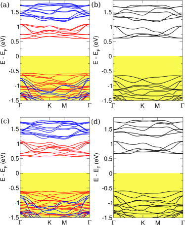
Figure 4: (Color online) Spin-polarized band structures of bilayer CrI₃ for (a) AB(FM), (b) AB(AF), (c) AA_1/3(FM) and (d) AA_1/3(AF).

VIII Discussion and conclusions.-

Our results provide a plausible explanation for two different experimental observations. First, the kink in the differential spin susceptibility $\frac{d\chi}{dT}$ observed in bulk CrI₃ at the structural phase transitionMcGuire et al. (2015). Second, the antiferromagnetic interlayer coupling observed for few-layer CrI₃ bilayers, at low temperatures Huang et al. (2017); Song et al. (2018); Klein et al. (2018); Huang et al. (2018). Given that in these experiments the CrI₃ layers are either deposited on a substrateHuang et al. (2017) or embedded in a circuit, we conjecture that the stacking might be different than in bulk. However, the confirmation of this hypothesis will require further experimental and computational work.

To summarize, we have computed the interlayer exchange for CrI₃ bilayers in two different stacking, that correspond to the rhombohedral and monoclinic structures observed for bulk CrI₃. We find that the interlayer coupling shows a much weaker ferromagnetic character for the monoclinic than the rhombohedral phase, and eventually undergoes an antiferromagnetic transition under shear strain. We claim that this provides a possible explanation for two different experimental observations. First, the kink observed in the differential susceptibility at the structural transition in bulk.McGuire et al. (2015) Second, the fact that CrI₃ bilayers deposited on graphene are known to have antiferromagnetic interlayer coupling.Huang et al. (2017); Wang et al. (2018); Song et al. (2018); Klein et al. (2018); Huang et al. (2018)

Note: During the final completion of this manuscript, we became aware of the work of four other groupsJiang et al. (2018); Sivadas et al. (2018); Jang et al. (2018) addressing the relation between interlayer exchange and stacking in CrI₃ using different approximations and obtaining results compatible with ours.

Acknowledgements.- We acknowledge Efrén Navarro-Moratalla for pointing out the different interlayer coupling for bilayer and bulk CrI₃. We thank José Luis Lado, Francisco Rivadulla , A. H. MacDonald and Jeil Jung for fruitful discussions. DS thanks NanoTRAINforGrowth Cofund program at INL and the financial support from EU through the MSCA Individual Fellowship program at Radboud University. J. F.-R. acknowledge financial support from FCT for the P2020-PTDC/FIS-NAN/4662/2014, the P2020-PTDC/FIS-NAN/3668/2014 and the UTAPEXPL/NTec/0046/2017 projects, as well as Generalitat Valenciana funding Prometeo2017/139 and MINECO Spain (Grant No. MAT2016-78625-C2). CC and JFR acknowledge FEDER project NORTE-01-0145-FEDER-000019. The authors thankfully acknowledge the computer resources at Caesaraugusta and the technical support provided by the Institute for Biocomputation and Physics of Complex Systems (BIFI) (RES-QCM-2018-2-0032). Part of this work was carried out on the Dutch national e-infrastructure with the support of SURF Cooperative.

References

- Gong et al. (2017) C. Gong, L. Li, Z. Li, H. Ji, A. Stern, Y. Xia, T. Cao, W. Bao, C. Wang, Y. Wang, et al., Nature 546, 265 (2017).
- Huang et al. (2017) B. Huang, G. Clark, E. Navarro-Moratalla, D. R. Klein, R. Cheng, K. L. Seyler, D. Zhong, E. Schmidgall, M. A. McGuire, D. H. Cobden, et al., Nature 546, 270 (2017).
- McGuire (2017) M. A. McGuire, Crystals 7, 121 (2017).
- Fei et al. (2018) Z. Fei, B. Huang, P. Malinowski, W. Wang, T. Song, J. Sanchez, W. Yao, D. Xiao, X. Zhu, A. May, et al., Nature materials 17, 778 (2018).
- O’Hara et al. (2018) D. J. O’Hara, T. Zhu, A. H. Trout, A. S. Ahmed, Y. K. Luo, C. H. Lee, M. R. Brenner, S. Rajan, J. A. Gupta, D. W. McComb, et al., Nano Letters 18, 3125 (2018).
- Song et al. (2018) T. Song, X. Cai, M. W.-Y. Tu, X. Zhang, B. Huang, N. P. Wilson, K. L. Seyler, L. Zhu, T. Taniguchi, K. Watanabe, et al., Science 360, 1214 (2018).
- Klein et al. (2018) D. R. Klein, D. MacNeill, J. L. Lado, D. Soriano, E. Navarro-Moratalla, K. Watanabe, T. Taniguchi, S. Manni, P. Canfield, J. Fernández-Rossier, et al., Science 360, 1218 (2018).
- Wang et al. (2018) Z. Wang, I. Gutiérrez-Lezama, N. Ubrig, M. Kroner, M. Gibertini, T. Taniguchi, K. Watanabe, A. Imamoğlu, E. Giannini, and A. F. Morpurgo, Nature Communications 9, 2516 (2018).
- Seyler et al. (2018) K. L. Seyler, D. Zhong, D. R. Klein, S. Gao, X. Zhang, B. Huang, E. Navarro-Moratalla, L. Yang, D. H. Cobden, M. A. McGuire, et al., Nature Physics 14, 277 (2018).
- Zhong et al. (2017) D. Zhong, K. L. Seyler, X. Linpeng, R. Cheng, N. Sivadas, B. Huang, E. Schmidgall, T. Taniguchi, K. Watanabe, M. A. McGuire, et al., Science Advances 3, e1603113 (2017).
- Huang et al. (2018) B. Huang, G. Clark, D. R. Klein, D. MacNeill, E. Navarro-Moratalla, K. L. Seyler, N. Wilson, M. A. McGuire, D. H. Cobden, D. Xiao, et al., Nature Nanotechnology 13, 544 (2018).
- Jiang et al. (2018a) S. Jiang, J. Shan, and K. F. Mak, Nature materials 17, 406 (2018a).
- Jiang et al. (2018b) S. Jiang, L. Li, Z. Wang, K. F. Mak, and J. Shan, Nature Nanotechnology 13, 549 (2018b).
- Lado and Fernández-Rossier (2017) J. L. Lado and J. Fernández-Rossier, 2D Materials 4, 035002 (2017).
- Liu et al. (2018a) J. Liu, M. Shi, J. Lu, and M. P. Anantram, Phys. Rev. B 97, 054416 (2018a).
- Liu and Petrovic (2018) Y. Liu and C. Petrovic, Phys. Rev. B 97, 014420 (2018).
- Richter et al. (2018) N. Richter, D. Weber, F. Martin, N. Singh, U. Schwingenschlögl, B. V. Lotsch, and M. Kläui, Phys. Rev. Materials 2, 024004 (2018).
- Zhang et al. (2018) J. Zhang, B. Zhao, T. Zhou, Y. Xue, C. Ma, and Z. Yang, Phys. Rev. B 97, 085401 (2018).
- Zollner et al. (2018) K. Zollner, M. Gmitra, and J. Fabian, New J. Phys. 20, 073007 (2018).
- Jiang et al. (2018c) P. Jiang, L. Li, Z. Liao, Y. Zhao, and Z. Zhong, Nano letters (2018c).
- Liu et al. (2018b) J. Liu, M. Shi, P. Mo, and J. Lu, AIP Advances 8, 055316 (2018b).
- Cardoso et al. (2018) C. Cardoso, D. Soriano, N. A. García-Martínez, and J. Fernández-Rossier, Phys. Rev. Lett. 121, 067701 (2018).
- Tong et al. (2018) Q. Tong, F. Liu, J. Xiao, and W. Yao, Nano Letters 18, 7194 (2018).
- Lee et al. (2019) I. Lee, F. G. Utermohlen, K. Hwang, D. Weber, C. Zhang, J. van Tol, J. E. Goldberger, N. Trivedi, and P. C. Hammel, arXiv e-prints arXiv:1902.00077 (2019), eprint 1902.00077.
- Besbes et al. (2019) O. Besbes, S. Nikolaev, and I. Solovyev, arXiv e-prints arXiv:1901.09525 (2019), eprint 1901.09525.
- Xu et al. (2018) C. Xu, J. Feng, H. Xiang, and L. Bellaiche, npj Computational Mathematics 4, 57 (2018), eprint 1811.05413.
- Morosin and Narath (1964) B. Morosin and A. Narath, The Journal of Chemical Physics 40, 1958 (1964).
- Handy and Gregory (1952) L. L. Handy and N. W. Gregory, Journal of the American Chemical Society 74, 891 (1952).
- McGuire et al. (2015) M. A. McGuire, H. Dixit, V. R. Cooper, and B. C. Sales, Chemistry of Materials 27, 612 (2015).
- Klein et al. (2019) D. R. Klein, D. MacNeill, Q. Song, D. T. Larson, S. Fang, M. Xu, R. A. Ribeiro, P. C. Canfield, E. Kaxiras, R. Comin, et al., arXiv e-prints arXiv:1903.00002 (2019), eprint 1903.00002.
- Thiel et al. (2019) L. Thiel, Z. Wang, M. A. Tschudin, D. Rohner, I. Gutiérrez-Lezama, N. Ubrig, M. Gibertini, E. Giannini, A. F. Morpurgo, and P. Maletinsky, arXiv e-prints arXiv:1902.01406 (2019), eprint 1902.01406.
- Goodenough (1955) J. B. Goodenough, Phys. Rev. 100, 564 (1955).
- Goodenough (1958) J. B. Goodenough, Journal of Physics and Chemistry of Solids 6, 287 (1958).
- Kanamori (1959) J. Kanamori, Journal of Physics and Chemistry of Solids 10, 87 (1959).
- Feldkemper and Weber (1998) S. Feldkemper and W. Weber, Phys. Rev. B 57, 7755 (1998).
- Giannozzi et al. (2009) P. Giannozzi, S. Baroni, N. Bonini, M. Calandra, R. Car, C. Cavazzoni, D. Ceresoli, G. L. Chiarotti, M. Cococcioni, I. Dabo, et al., Journal of Physics: Condensed Matter 21, 395502 (2009).
- Perdew et al. (1996) J. P. Perdew, K. Burke, and M. Ernzerhof, Physical review letters 77, 3865 (1996).
- Grimme (2006) S. Grimme, Journal of computational chemistry 27, 1787 (2006).
- Jiang et al. (2018) P. Jiang, C. Wang, D. Chen, Z. Zhong, Z. Yuan, Z.-Y. Lu, and W. Ji, ArXiv e-prints (2018), eprint 1806.09274.
- Sivadas et al. (2018) N. Sivadas, S. Okamoto, X. Xu, C. J. Fennie, and D. Xiao, Nano Letters 18, 7658 (2018).
- Jang et al. (2018) S. W. Jang, M. Y. Jeong, H. Yoon, S. Ryee, and M. J. Han, ArXiv e-prints (2018), eprint 1809.01388.
- Lei et al. (2019) C. Lei, B. Lingam Chittari, K. Nomura, N. Banerjee, J. Jung, and A. H. MacDonald, arXiv e-prints arXiv:1902.06418 (2019), eprint 1902.06418.
- Anisimov et al. (1991) V. I. Anisimov, J. Zaanen, and O. K. Andersen, Physical Review B 44, 943 (1991).
- Anderson (1963) P. W. Anderson (Academic Press, 1963), vol. 14 of Solid State Physics, pp. 99 – 214.
- Hay et al. (1975) P. J. Hay, J. C. Thibeault, and R. Hoffmann, Journal of the American Chemical Society 97, 4884 (1975).
- Mostofi et al. (2014) A. A. Mostofi, J. R. Yates, G. Pizzi, Y. S. Lee, I. Souza, D. Vanderbilt, and N. Marzari, Comput. Phys. Commun. 185, 2309 (2014).