Towards Adversarial Training with Moderate Performance Improvement for Neural Network Classification

Abstract

It has been demonstrated that deep neural networks are prone to noisy examples particular adversarial samples during inference process. The gap between robust deep learning systems in real world applications and vulnerable neural networks is still large. Current adversarial training strategies improve the robustness against adversarial samples. However, these methods lead to accuracy reduction when the input examples are clean thus hinders the practicability. In this paper, we investigate an approach that protects the neural network classification from the adversarial samples and improves its accuracy when the input examples are clean. We demonstrate the versatility and effectiveness of our proposed approach on a variety of different networks and datasets.

1 Introduction

Many high-performance deep learning applications in computer vision, speech recognition and other areas are susceptible to minimal changes of the inputs He et al. (2018). Therefore, a robust system is required for the real-world applications when the input is affected by many interferences and noise.

Current robust learning strategies in the context of neural network classification only play against adversarial samples, while the accuracy reduces when the samples are clean. In this paper, we stand on the perspective of robust optimization and propose an approach to improve the performance of the networks on both clean and noise data. In particular, we propose a counterpart of the FSGM algorithm (Goodfellow et al. (2014)), which inherits the sign function for the robustness against permutation and helps the neural network leaves saddle points during the training process.

2 Related Work

Adversarial training strategies are proposed for both attacks and defenses inspired by robust optimization. For example, a training procedure is provided that model parameters updates are augmented with the worst-case perturbations of the training data Sinha et al. (2017). A mixed strategy named stochastic activation pruning (SAP) is applied on the training of deep neural networks for the robustness against adversarial examples in He et al. (2018). A potential application of local intrinsic dimensionality is studied to distinguish adversarial examples Ma et al. (2018). These adversarial training strategies are presented with better performance when the input examples are noisy. However, the above algorithms do not perform well when the input samples are free from noise. In the following, we introduce an algorithm that is capable to improve the performance without any assumption on the data quality.

3 Methodology

In a standard deep learning task, we let $f$ denote the complex non-linear function of the deep neural network and $\theta$ denote the parameters of $f$. Let $x$ and $y$ be the input and output sample of the network. $y=f(x)$ denotes the standard function of a deep learning task. We use $sgn$ to denote the sign function and use $\delta(x)$ to define the dirac delta function. We use $\it{D}$ to represent the data distribution over pairs of examples $x\in\mathbb{R}^{d_{1}}$ and labels $y\in\mathbb{R}^{d_{2}}$. Denote $L(\theta,x,y)$ as the loss function, and the goal is to find model parameters $\theta$ that minimize the risk $\mathbb{E}_{(x,y)}[L(\theta,x,y)]$. This empirical risk minimization (ERM) is successful for finding classifiers with small population task. However, it is not robust enough against some common disturbances. In particular, the model incorrectly classifies $\hat{x}$ as belonging to a different class of $x$ if $\hat{x}$ is very close to $\hat{x}$.

In order to impose robustness, the population risk $\mathbb{E}_{\it{D}}[L]$ is formulated as the following

$$\rho(\theta)=\mathbb{E}_{(x,y)\sim\it{D}}\left[\max_{\delta\in\it{S}}L(\theta,x+\delta,y)\right].\\$$ (1)

The objective is to minimize the above population risk

$$\min{\rho(\theta)}.$$

We next define $g(x)$ to be the function which produces adversarial samples from clean samples. That is, $\hat{x}=g(x)$. The population risk $\mathbb{E}_{\it{D}}[L]$ is represented as $\rho(\theta)=\mathbb{E}_{(x,y)\sim\it{D}}\left[\max_{\delta\in\it{S}}L(\theta,g(x),y)\right]$. The corresponding function is denoted as $y=f(g(x))$. In the following, we first propose an algorithm, and analyzed the Jacobian of the deep neural network when the algorithm is applied. We further analyze the Hessian. Based on the analysis, we could safely say that the proposed algorithm dose not introduce extra saddle points and may be very likely help the neural network leave saddle points on a sharper direction of the loss function surface.

3.1 Analysis of Jacobian

We propose the following algorithm:

$$g(x)=x+\epsilon xsgn(x).$$

We have

$$\frac{\partial g(x)}{\partial x}=1+\epsilon(sgn(x)+x\delta^{\prime}),$$

$$\frac{\partial^{2}g(x)}{\partial x^{2}} =\epsilon(\delta(x)+\delta(x)+x\delta^{\prime}(x))$$

$$=\epsilon(\delta(x)+\delta(x)-\delta(x))$$

$$=\epsilon\delta(x)$$

Firstly, the Jacobian is given as following.

$$J(\theta) =\frac{\partial f(g(x))}{\partial x}$$

$$=\frac{\partial f(x)}{\partial x}(1+\epsilon(sgn(x)+x\delta^{\prime}))$$

$$=\frac{\partial f(x)}{\partial x}(1+\epsilon sgn(x))$$

If $\epsilon$ is smaller than $1$, no extra extreme points will be introduced. The extreme points are all from $\frac{\partial f(x)}{\partial x}=0$.

3.2 Analysis of Hessian

The Hessian is given as following.

$$H(\theta)= \frac{\partial^{2}f(g(x))}{\partial x^{2}}$$

$$= \frac{\partial^{2}f(x)}{\partial x^{2}}\frac{\partial g(x)}{\partial x}\frac{\partial g(x)}{\partial x}+\frac{\partial f(x)}{\partial x}\frac{\partial^{2}g(x)}{\partial x^{2}}$$

$$= \frac{\partial^{2}f(x)}{\partial x^{2}}(1+\epsilon(sgn(x)+x\delta(x)))^{2}+\frac{\partial f(x)}{\partial x}(\epsilon\delta(x))$$

For any extreme points such that $\frac{\partial f(x)}{\partial x}=0$, the Hessian equation is given by

$$\newline H(\theta)=\frac{\partial^{2}f(x)}{\partial x^{2}}(1+\epsilon^{2}sgn(x)sgn(x)).$$

It could be observed that the change rate of the Jacobian is increased as $1+\epsilon^{2}sgn(x)sgn(x)\geq 1$. This implies a higher rate of change which helps the neural networks leave saddle points during the training process.

3.3 Implementation

The proposed $g(x)$ could be applied in the input space and the hidden space of the deep neural networks. That is, $x$ could be samples of the input and the vectors in the hidden space of the deep neural networks.

In order to apply the adversarial training strategy on-line without extra computational burden, the proposed algorithm dose not rely on the calculation of gradients like FGSM (Goodfellow et al. (2014)). Instead, the perturbation item is calculated feed-forward once the samples in the input/hidden space are calculated.

Let $x$ denote the samples in the input/hidden space. In the following experiments, $g(x)$ has the form

$$g(x)=x+\epsilon x\odot l(x).$$

Here

$$\left\{\begin{array}[]{lr}l(x)=sgn(x)\quad w.p.\quad p,&\\ l(x)=-sgn(x)\quad w.p.\quad 1-p.\\ \end{array}\right.$$

4 Numerical experiments

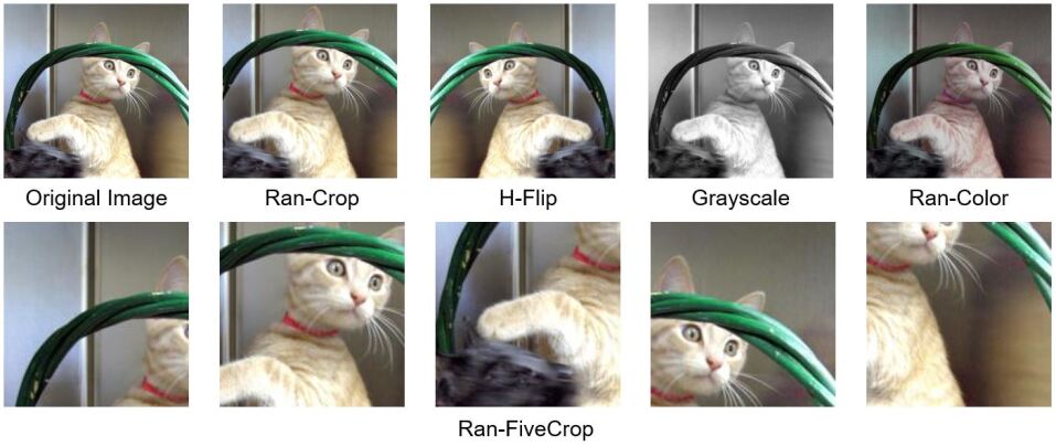
Figure 1: Five common attacks.

Table 1: Top-1 classification accuracy on ImageNet-1k for five different disturbances in the input space.

Model Ran-Crop Ran-Hlip Ran-GrayScale(%) Ran-Color(%) Random Five Crop(%) Imagenet FGSM-CondenseNet(G=C=8) 68.27 69.42 68.03 69.21 58.17 CondenseNet(G=C=8) $70.04\pm 0.05$ $71.00\pm 0.03$ $69.79\pm 0.04$ $71.05\pm 0.04$ $60.03\pm 0.05$ R-CondenseNet(G=C=8) $\textbf{70.38}\pm{0.03}$ $\textbf{71.29}\pm{0.05}$ $\textbf{70.06}\pm{0.03}$ $\textbf{71.25}\pm{0.02}$ $\textbf{60.45}\pm{0.04}$ FGSM-CondenseNet(G=C=4) 70.34 71.48 70.72 71.39 60.04 CondenseNet(G=C=4) 7$2.92\pm{0.02}$ $73.78\pm{0.05}$ $72.74\pm{0.03}$ $73.76\pm{0.03}$ $62.52\pm{0.04}$ R-CondenseNet(G=C=4) $\textbf{73.34}\pm 0.03$ $\textbf{74.12}\pm 0.02$ $\textbf{73.05}\pm 0.05$ $\textbf{74.07}\pm 0.06$ $\textbf{63.26}\pm 0.04$

Table 2: Top-1 and Top-5 classification accuracies of state-of-art regular models on ImageNet-1k.

Model Image Size Params Mul-Adds Tops-1(%) Tops-5(%) Imagenet SENet $320\times 320$ 145.8M 42.4B 82.7 96.2 NASNet-A $331\times 331$ 88.9M 23.8B 82.7 96.2 FGSM-NASNet-A $331\times 331$ 88.9M 23.8B 80.6 92.1 R-NASNet-A $331\times 331$ 88.9M 23.8B $\textbf{83.0}\pm\textbf{0.03}$ $\textbf{96.5}\pm\textbf{0.05}$

Table 3: Top-1 and Top-5 classification error rate of state-of-art compact models on ImageNet-1k.

Model FLOPs Params Tops-1(%) Tops-5(%) Imagenet Inception V1 1,448M 6.6M 30.2 10.1 1.0 MobileNet-224 569M 4.2M 29.4 10.5 ShffleNet 2x 524M 5.3M 29.1 10.5 NASNet-B(N=4) 488M 5.3M 27.2 9.0 NASNet-C(N=3) 558M 4.9M 27.5 9.0 CondenseNet(G=C=8) 274M 2.9M 29.0 10.0 CondenseNet(G=C=4) 274M 2.9M 26.2 8.3 FGSM-CondenseNet(G=C=8) 274M 2.9M 30.8 12.3 FGSM-CondenseNet(G=C=4) 529M 4.8M 27.9 10.7 R-CondenseNet(G=C=8) 274M 2.9M $\textbf{28.6}\pm\textbf{0.05}$ $\textbf{9.9}\pm\textbf{0.06}$ R-CondenseNet(G=C=4) 529M 4.8M $\textbf{25.8}\pm\textbf{0.04}$ $\textbf{8.1}\pm\textbf{0.05}$

Table 4: Middle-scaled supervised classification: MNIST and SVHN.

Model Depth Factor Dropout Standard Aug Random Erase Error(%) MNIST LeNetLeCun et al. (1998) - - $\surd$ - - 0.50 FGSM-LeNet - - $\surd$ - - 0.60 R-LeNet - - $\surd$ - - 0.28 CapsNetSabour et al. (2017) - - $\surd$ - - 0.35 FGSM-CapsNet - - $\surd$ - - 0.51 R-CapsNet - - $\surd$ - - 0.30 SVHN S-ResNet Huang et al. (2016) 110 - $\surd$ $\surd$ - 1.75 FGSM-S-ResNet 110 - $\surd$ $\surd$ - 1.90 R-S-ResNet 110 - $\surd$ $\surd$ - 1.70 W-ResNet Zagoruyko and Komodakis (2016) 16 k = 8 $\surd$ $\surd$ - 1.54 FGSM-S-Resnet 16 k = 8 $\surd$ $\surd$ - 1.71 R-W-ResNet 16 k = 8 $\surd$ $\surd$ - 1.49

Table 5: Middle-scaled supervised classification: CIFAR10 and CIFAR100.

Model Depth Factor Dropout Standard Aug Random Erase Error(%) CIFAR10 W-ResNet Zagoruyko and Komodakis (2016) 28 k = 10 $\surd$ $\surd$ $\surd$ 3.1 FGSM-W-ResNet 28 k = 10 $\surd$ $\surd$ $\surd$ 4.2 R-W-ResNet 28 k = 10 $\surd$ $\surd$ $\surd$ 2.7 CIFAR100 InceptionV3 Szegedy et al. (2015) 48 - $\surd$ $\surd$ - 22.69 FGSM-InceptionV3 48 - $\surd$ $\surd$ - 23.41 R-InceptionV3 48 - $\surd$ $\surd$ - 21.80 W-ResNet Zagoruyko and Komodakis (2016) 28 k = 10 $\surd$ $\surd$ $\surd$ 17.73 FGSM-W-ResNet 28 k = 10 $\surd$ $\surd$ $\surd$ 18.61 R-W-ResNet 28 k = 10 $\surd$ $\surd$ $\surd$ 17.18

We evaluate the proposed form of robust algorithm $g(x)$ where $p=0.5$. The evaluation is made on a variety of popular datasets, including small-scale, middle-scale and large-scale datasets (MNIST LeCun et al. (1998), CIFAR10, CIFAR100 Krizhevsky and Hinton (2009), SVHN Netzer et al. (2011) and Imagenet-1k Russakovsky et al. (2015)). Extensive experimental evaluations are presented in two aspects including performance improvement for the clean samples in input space and the noisy samples in input space (see Figure 1). We evaluate the FGSM for base models and the proposed algorithm for based models, called R-base models. As shown in Table 1, the accuracy is improved when the inputs are noisy compared with base models and FGSM for base models. As shown in Table 2 to Table 5, the accuracy is improved when the inputs are clean.

5 Discussion

We propose an approach that help neural networks achieve both robustness against noisy inputs and higher accuracy for clean input. It enhances the practicality of neural networks such that the input can be clean or noisy.

This is an initial work that only five common types of noise are evaluated. In the real world, the types of noise are unknown and it remains unclear whether the inputs is attacked by the disturbance or not. In addition, the base model is also a black box that the gradients are hard to obtain. A systematic way of overcoming these problems deserve one’s attention.

References

- Goodfellow et al. [2014] Ian J Goodfellow, Jonathon Shlens, and Christian Szegedy. Explaining and harnessing adversarial examples. arXiv preprint arXiv:1412.6572, 2014.
- He et al. [2018] Warren He, Bo Li, and Dawn Song. Decision boundary analysis of adversarial examples. In ICLR-International Conference on Learning Representations, 2018.
- Huang et al. [2016] Gao Huang, Yu Sun, Zhuang Liu, Daniel Sedra, and Kilian Q Weinberger. Deep networks with stochastic depth. In European Conference on Computer Vision, pages 646–661. Springer, 2016.
- Krizhevsky and Hinton [2009] Alex Krizhevsky and Geoffrey Hinton. Learning multiple layers of features from tiny images. 2009.
- LeCun et al. [1998] Yann LeCun, Léon Bottou, Yoshua Bengio, and Patrick Haffner. Gradient-based learning applied to document recognition. Proceedings of the IEEE, 86(11):2278–2324, 1998.
- Ma et al. [2018] Xingjun Ma, Bo Li, Yisen Wang, Sarah M Erfani, Sudanthi Wijewickrema, Michael E Houle, Grant Schoenebeck, Dawn Song, and James Bailey. Characterizing adversarial subspaces using local intrinsic dimensionality. arXiv preprint arXiv:1801.02613, 2018.
- Netzer et al. [2011] Yuval Netzer, Tao Wang, Adam Coates, Alessandro Bissacco, Bo Wu, and Andrew Y Ng. Reading digits in natural images with unsupervised feature learning. In NIPS workshop on deep learning and unsupervised feature learning, volume 2011, page 5, 2011.
- Russakovsky et al. [2015] Olga Russakovsky, Jia Deng, Hao Su, Jonathan Krause, Sanjeev Satheesh, Sean Ma, Zhiheng Huang, Andrej Karpathy, Aditya Khosla, Michael Bernstein, et al. Imagenet large scale visual recognition challenge. International Journal of Computer Vision, 115(3):211–252, 2015.
- Sabour et al. [2017] Sara Sabour, Nicholas Frosst, and Geoffrey E Hinton. Dynamic routing between capsules. arXiv preprint arXiv:1710.09829, 2017.
- Sinha et al. [2017] Aman Sinha, Hongseok Namkoong, and John Duchi. Certifiable distributional robustness with principled adversarial training. arXiv preprint arXiv:1710.10571, 2017.
- Szegedy et al. [2015] Christian Szegedy, Wei Liu, Yangqing Jia, Pierre Sermanet, Scott Reed, Dragomir Anguelov, Dumitru Erhan, Vincent Vanhoucke, and Andrew Rabinovich. Going deeper with convolutions. In Proceedings of the IEEE conference on computer vision and pattern recognition, pages 1–9, 2015.
- Zagoruyko and Komodakis [2016] Sergey Zagoruyko and Nikos Komodakis. Wide residual networks. In Edwin R. Hancock Richard C. Wilson and William A. P. Smith, editors, Proceedings of the British Machine Vision Conference (BMVC), pages 87.1–87.12. BMVA Press, September 2016.