Data-driven satisficing measure and ranking

Abstract

We propose an computational framework for real-time risk assessment and prioritizing for random outcomes without prior information on probability distributions. The basic model is built based on satisficing measure (SM) which yields a single index for risk comparison. Since SM is a dual representation for a family of risk measures, we consider problems constrained by general convex risk measures and specifically by Conditional value-at-risk. Starting from offline optimization, we apply sample average approximation technique and argue the convergence rate and validation of optimal solutions. In online stochastic optimization case, we develop primal-dual stochastic approximation algorithms respectively for general risk constrained problems, and derive their regret bounds. For both offline and online cases, we illustrate the relationship between risk ranking accuracy with sample size (or iterations).

Keywords: Risk measure; Satisficing measure; Online stochastic optimization; Stochastic approximation; Sample average approximation; Ranking;

1 Introduction

Risk assessment is the process where we identify hazards, analyze or evaluate the risk associated with that hazard, and determine appropriate ways to eliminate or control the hazard. Risk assessment techniques have been widely applied in many area including quantitative financial engineering (Krokhmal et al., 2002), health and environment study (Zhang and Wang, 2012; Van Asselt et al., 2013), transportation science (Liu et al., 2017), etc. Paltrinieri et al., (2014) point out that traditional risk assessment methods are often limited by static, one-time processes performed during the design phase of industrial processes. As such they often use older data or generic data on potential hazards and failure rates of equipment and processes and cannot be easily updated in order to take into account new information, giving a more complete view of the related risks. This failure to account for new information can lead to unrecognized hazards, or misunderstandings about the real probability of their occurrence under current management and safety precautions. With the rapid development of computational intelligence and corresponding decision support system, as well as the launch of “Big data” era, nowadays, new risk assessment technique should allow decision maker to update the assessment results by observing new information or data and realize quick response to dynamic environment. In this paper, we develop a satisficing measure based model to assess, compare and ranking random outcomes, and propose both online and offline data-driven computational frameworks. We validate the methods both theoretically and experimentally. The title of this paper “Data-driven” means that the probability distribution of the randomness is not available in our settings, and we conduct risk assessment and ranking, only based on observed empirical data.

The core of real-time assessment allows us to update the assessment results by observing new information or data and realize quick response to dynamic environment. Two most commonly used real-time assessment techniques are Hidden Markov model (HMM) and Bayesian network introduced by Ghahramani, (2001). HMM models used in Tan et al., (2008); Li and Guo, (2009); Yu-Ting et al., (2014); Haslum and Årnes, (2006) can combine both external and internal threats in network security systems, and the experiment results show that such method can improve the accuracy and reliability of assessment than the statics approaches. Bayesian approaches used in Sandoy and Aven, (2006) can solve problems generated by introducing or not introducing an underlying probability model. The pairwise comparison theory (also called Bradley-Terry-Luce (BTL) model) widely used in study the preference in decision making was introduced in Bradley and Terry, (1952); Luce, (2005). A Bayesian approximation method with BTL model in Weng and Lin, (2011), is proposed for online ranking in team performance. However, these methodologies do not consider assessing the “risk” of the systems and have not provided a formal definition of risk that can be uniformly applied to wide range of systems.

In financial mathematics, “risk measure” is defined as a mapping function from a probability space to real number. Some fundamental research has been conducted motivating the definition of risk measure. In Ruszczynski and Shapiro, (2006), the definitions and conditions for convex and coherent risk measures are developed, and conjugate duality reformulation of risk functions is proposed. Rockafellar and Uryasev, (2000) give the detailed arguments on the most widely investigated coherent and law invariant risk measure-Conditional value-at-risk (CVaR) with corresponding reformulation and optimization problem illustration. CVaR is widely involved in optimization under uncertainty, and helps to improve the reliability of solutions against extremely high loss. Krokhmal et al., (2002) study the portfolio optimization problem with CVaR objective and constraints, and corresponding reformulation and discretization are demonstrated. In Dai et al., (2016), robust version CVaR is applied in portfolio selection problem, where sampled scenario returns are generated by a factor model with some asymmetric and uncertainty set. In Noyan and Rudolf, (2013), multivariate CVaR constraint problem is studied based on polyhedral scalarization and second-order stochastic dominance, and a cut generation algorithm is proposed, where each cut is obtained by solving a mixed integer problem. Xu and Yu, (2014) reformulate a stochastic nonlinear complementary problem with CVaR constraints, and propose a penalized smoothing sample average approximation algorithm to solve the CVaR-constrained stochastic programming. Shapiro, (2013) gives Kusuoka representation of law invariant risk measures. The basic idea is to use a class of CVaR constraints to formulate any coherent and law invariant risk measure.

In practice, the above classical risk measures have shortcomings in real applications. First, classical risk measures like CVaR require the decision maker to specify his own risk tolerance parameters in order to accurately capture the risk preference of decision maker as well as provide an exact mathematical formulation of risk. However, this process is very different to realize in practice, mentioned in Delage and Li, (2015); Armbruster and Delage, (2015). Secondly, we consider that the “risk” of random variables are compared, based on metric on how the random outcome exceeds certain risk measure. If the random outcome exceeds the risk measure, we consider these outcomes are in risky region. Obviously, classical risk measures are not appropriate for conducting risk comparison for random outcomes under different probability distributions. For example, suppose random variable $X$ dominates $Y$ in first-order. We can conjuncture that there exist realizations of $X$ and $Y$, such that realizations of $X$ has higher value than realization of $Y$, but realization of $Y$ exceeds its value-at-risk while realization $X$ does not. Thus, comparing the value of risk measure is failed to identify which random variable is more “risky”. Thus, new models are required specifically for risk assessment and comparison.

Recently, new metrics on risk are developed including satisficing measure and aspirational preference measure. In Brown and Sim, (2009), satisficing measure evaluating the quality of financial positions based on their ability to achieve desired financial goals can be show to be dual to a class of risk measures. Such target are often much more natural to specify than risk tolerance parameters, and ensure robust guarantees. InBrown et al., (2012), Aspirational preference measure is developed as an expanded case for satisficing measure that can handle ambiguity without a given probability distribution, moreover, it possesses more general properties than satisficing measure. These target-based risk measures yield a single index to metric the risk of random outcomes. Besides, the index are normally contained in a fixed and closed interval, which can be used to rank the risk of random outcomes. In Chen et al., (2014), satisficing measure is applied in studying the impact of target on newsvendor decision. For practical use, there still exists space for improvement for satisficing measure. First, current measures are developed based on some simple and specific risk measures like CVaR, rather than adapt themselves to general convex or coherent risk measures. Second, the models rely on the full knowledge of the probability distribution of the random variable, which are hard to collect in practice. To make the full potential of these models for practical use, in this paper, we follow the ideas in Postek et al., (2015); Ben-Tal and Teboulle, (2007), derive computationally tractable counterparts of distributionally robust constraints on risk measures, by using the optimized certainty equivalent framework. Thus we provide a general formulation of satisficing measures that can cover range of risk measures.

Lacking the information of probability distribution of uncertainty is normally an important issue in risk management and robust optimization. Delage and Ye, (2010) connect distributionally robust optimization with data-driven techniques, and propose a model that describes uncertainty in both the distribution form (discrete, Gaussian, exponential, etc.) and moments (mean and co-variance matrix). Brown et al., (2006) provides a comprehensive and integrated view between convex and coherent risk measure with robust optimization, and provide probability guarantee centered on data-driven approach. Instead of using data to estimate the uncertainty set, we derive the robust counterpart of distributionally robust formulation of risk, and then adopt online stochastic optimization (see Bubeck, 2011; Shalev-Shwartz, 2011) approach for data-driven optimization. Such computational framework is more efficient and easy to analyze the theoretical properties. Research has been done in extending online unconstrained stochastic optimization methods in constrained optimization or risk-aware optimization. In Mahdavi et al., (2012), online stochastic optimization with multiple objective is studied, the idea is to cast the stochastic multiple objective optimization problem into a constrained optimization problem by choosing one function as the objective and try to bound other objectives by appropriate thresholds. Projected gradient method and efficient primal-dual stochastic algorithm are developed to tackle such problem. In Duchi et al., (2011), a new family of subgradient methods has been presented that dynamically incorporate knowledge of the geometry of the data observed in earlier iterations to perform more informative gradient-based learning. In Bardou et al., (2009), stochastic approximation approach has been applied to estimate CVaR in data-driven optimization problems. Moreover, in Carbonetto et al., (2009), studies has been conducted to develop stochastic interior-point algorithm to solve constrained problem. In this paper, our online algorithm extends the stochastic approximation of CVaR in Bardou et al., (2009) to constrained optimization problem with general convex risk measures.

In this paper, we develop a general framework for data-driven risk assessment and ranking. The key contributions lay in three aspects.

1. We build a risk constrained satisficing measure model which can yield a single index for risk comparison. Using optimized certainty equivalent formulation, our model can cover a wide range of risk measures.

2. Without knowledge on the probability distribution, our data-driven computational methods are developed only based on observations. We consider both in offline and online cases. In offline case, sample average approximation (SAA) approach were applied to perform convergence analysis for the feasible region and validation analysis for optimal solution. In online case, we develop a primal-dual algorithm to solve the problem. We figure out the regret bound and its relationship with iteration number.

3. We check the validation of risk ranking results both in offline and online cases. Explicitly, we want to check given all the information of a batch of random variables and their true risk ranking. How close is the ranking computed from data-driven method to the true ranking. As the sample size grows, we show the convergence rate of ranking results from SAA and online algorithm to the true underlying result in probability.

The remainder of the paper is organized as follows. In Section 2 we establish the necessary preliminaries and introduce some basic methodologies. Section 3 illustrates the general model for offline problem, sample average approximation analysis, and validation of offline ranking results. Section 4 presents efficient primal-dual algorithm to solve online risk assessment problem, with validation of online ranking results. Finally, we conclude the paper with open questions in Section 5.

2 Preliminaries

This section introduces preliminary concepts and notation to be used throughout the paper.

2.1 Risk measure

Define a certain probability space $(\Omega,\mathcal{F},\,P_{0})$, where $\Omega$ is a sample space, $\mathcal{F}$ is a $\sigma-$algebra on $\Omega$, and $P_{0}$ is a probability measure on $(\Omega,\mathcal{\,F})$ . We concern throughout with random variables in $\mathcal{L}=L_{\infty}(\Omega,\mathcal{\,F},\,P_{0})$, the space of essentially bounded $\mathcal{F}-$measurable functions. if let $\mathcal{X}$ denote the linear space of $\mathcal{F}-$measurable functions $X:\,\Omega\rightarrow\mathbb{R}$. We first define concept of risk measure based on the definition in Ruszczynski and Shapiro, (2006) as a function $\rho$, which assigns to an uncertain random variable $X$ a real value $\mu(X)$. Formally,

A risk measure is a mapping $\rho:\mathcal{X}\rightarrow\mathbb{R\cup}\{+\infty\}\cup\{-\infty\}$ if $\mu(0)$ is finite and if $\mu$ satisfies the following conditions for all $X,\,Y\in\mathcal{X}.$ For $X,\,Y\in\mathcal{X},$ the notation $Y\succeq X$ means that $Y\text{($\omega$)$\geq$$X(\omega)$}$ for all $\omega\in\Omega$. The following four properties of risk functions are important throughout our analysis:

(A1) Monotonicity: If $Y\succeq X$, then $\rho(X)\geq\rho(Y)$.

(A2) Transition Invariance: If $r\in\mathbb{R}$, then $\rho(X+r)=\rho(X)-r.$

(A3) Convexity: $\rho(\lambda X+(1-\lambda)Y)\leq\lambda\rho(X)+(1-\lambda)\rho(Y),$ for $0\leq\lambda\leq 1.$

(A4) Positive Homogeneity: If $\lambda\geq 0$, then $\rho(\lambda X)=\lambda\rho(X).$
These conditions were introduced, and real valued functions $\rho:$ $\mathcal{X}\rightarrow\mathbb{R}$ satisfying (A1)-(A4) were called coherent measures of risk in the pioneering paper (Artzner et al., 1999). In fact, (A3) is equivalent to weaker requirement called Quasi convexity: $\rho(\lambda X+(1-\lambda)Y)\leq\max(\rho(X),\,\rho(Y))$, for $0\leq\lambda\leq 1$, when the risk measure is positive homogeneous. This property reveals the “diversification” preference of actual decision maker. Recall that a risk measure is law invariant if it only depends on the distributions of the random variables in question and not on the underlying probability space, i.e.

$$\rho(X)=\rho(Y),\,\forall X=_{D}Y,$$

where $=_{D}$ denotes equality in distribution. We present general convex risk measure into distributionally robust formulation based on the definition in Ruszczynski and Shapiro, (2006). The distributionally robust formulation of risk measure enables us to construct any risk measure on probability space $\mathcal{L}$ by choosing different convex and proper function embedded in the risk measure. Given a probability space $\mathcal{L}_{p}(\Omega,\,\mathcal{F},\,P)$ is associated with its dual space $\mathcal{L}_{q}(\Omega,\,\mathcal{F},\,P)$, satisfying $q\in(1,+\infty]$ and $1/p+1/q=1$. For $\omega\in\Omega$, $X\in\mathcal{L}_{p}$ and $Q\in\mathcal{L}_{q}$, the expectation is defined by their scalar product as

$$\mathbb{E}^{Q}[X]=\int_{\Omega}Q(\omega)X(\omega)dP(\omega).$$

Based on the results derived in Föllmer and Schied, (2011); Föllmer and Knispel, (2013), it is proved that any convex risk measure $\rho$ on random outcome $X$ can be represented into a robust representation as

$$\rho(X)=\sup_{Q\in\mathcal{P}}\left\{\mathbb{E}^{Q}[X]-h(Q)\right\},$$ (1)

where$\mathcal{P}$ is the set of all probability measures on $\Omega$, and function $h:\mathcal{L}_{q}\rightarrow\mathbb{R}$ is a proper and convex penalty function on $\mathcal{P}$ satisfying $\inf_{Q\in\mathcal{P}}h(Q)=0$, if $\rho$ is proper, lower semicontinuous, and convex function. When $h(Q)=0,\,\forall Q\in\mathcal{P}$, then any coherent risk measure can be represented by (1), i.e.

$$\rho(X)=\sup_{Q\in\mathcal{P}}\,\mathbb{E}^{Q}[X].$$

2.2 Target-based measure

Target-based decision making is first investigated in Simon, (1955, 1959) where the concept of satisficing and aspirational levels are introduced to evaluate the preference and action of decision makers. Recently new risk measures developed in literature that are able to evaluate the quality of positions with random outcomes based on their ability to achieve desired target in Shalev, (2000); Sugden, (2003); De Giorgi and Post, (2011); Kőszegi and Rabin, (2006). Satisficing measure proposed by Brown and Sim, (2009) is the most recent invention of target-based measure. Moreover, this paper further implies that optimization of these measures can be approached using computationally tractable tools from convex optimization, in contrast to the difficult, combinatorial problems that plague optimization of value-at-risk and related measures. Finally, these satisficing measures have a separation property which allows us to compute a single “tangent” portfolio regardless of the desired expected value. Such value is quite useful for risk comparison and ranking. The definition of satisficing measure we use is from Brown and Sim, (2009, Definition 1). Let $(\Omega,\mathcal{\,F},\,P)$ be a probability space and let $\mathcal{\mathcal{L}}$ be a set of random variable on $\Omega$. The decision maker has an aspiration level $\tau$ as an target. Given an uncertain payoff $X\in\mathcal{\mathcal{L}}$, define target premium $V$ to be the excess payoff above $\tau$, i.e., $V=X-\tau\in\mathcal{V}$. We assume that $\mathcal{V=\mathcal{L}}$. In other words, we will assume each of the payoffs $X\in\mathcal{L}$ already has the aspiration level embedded within it, and suppress the notation $\tau$ in the following definition.

Definition 2.1.

A function $\mu:\,\mathcal{\mathcal{L}\rightarrow}[0,\,\bar{p}],$ where $\bar{p}\in\left\{1,\,\infty\right\},$ is a satisficing measure defined on the target premium if it satisfies the following axioms for all $X,\,Y\in\mathcal{L}$:

• Attainment content: If $X\geq 0$, then $\mu(X)=\bar{p.}$

• Non-attainment apathy: If $X<0$, then $\mu(X)=0.$

• Monotonicity: If $X\geq Y,$ then $\mu(X)\geq\mu(Y).$

• Gain continuity: $\lim_{a\rightarrow 0^{+}}\mu(X+a)=\mu(X).$

Traditional risk measure like Conditional value-at-risk derives a mapping that yields a risk outcome of random variable based on certain quantile level; however, the risk measure and comparison result will varies by selecting different quantile level, while a more natural approach is to provide a framework for measuring the quality of risky positions with respect to their ability to satisfy a certain target $\tau$, as a metric for measuring how “risky” a random outcomes is. This concept has the advantage that aspiration levels are often natural for decision makers to specify, as opposed to the risk-tolerance type parameters, which can be difficult to intuitively understand and hard to appropriately specify, that are necessary for many other approaches (risk measures, utility functions, etc.). Moreover, the optimal satisficing value is normalized in a bounded interval, usually $[0,\,1]$, which is natural and convenient to illustrate the ranking result. Finally, any satisficing measure can be reformulated mathematically as a dual problem of its corresponding risk measure, so that in Brown et al., (2012), aspirational preference measure is developed as an expanded case for satisficing measure that can handle ambiguity without a given probability distribution; moreover, it possesses more general properties than satisficing measure. Computationally, these two risk metrics lead to the topics on solving risk constrained optimization problems, for example, CVaR constrained problem.

3 Model

In this section, we develop the general satisficing measure and ranking model. Rockafellar and Uryasev, (2013) introduce the concept called Risk quadrangle that any risk measure can be portrayed on a higher level as generated from penalty-type expressions of “regret” about the mix of potential outcomes. Specifically, define $(\Omega,\mathcal{\,F},\,P)$ be a probability space, let $\mathcal{\mathcal{L}}$ be a set of random variable on $\Omega$, and the random variable $X\in\mathcal{L}$. Then any risk measure can be defined as following trade-off formula.

$$\mu(X)=\min_{C\in\mathbb{R}}\left\{C+\mathcal{\mathcal{U}}(X-C)\right\},$$

Where $\mathcal{U}$ is mapping $\mathcal{L}\rightarrow\mathbb{R}$, called measure of regret. Regret comes up in penalty approaches to constraints in stochastic optimization and, in mirror image, corresponds to measures of utility. We first recall a class of certainty equivalents introduced in Ben-Tal and Teboulle, (1986), and further developed in Ben-Tal and Teboulle, (2007) that represents the specific application of the idea of Risk quadrangle which provides a wide family of risk measures that fits the axiomatic formalism of convex risk measures. We first introduce the following definition.

Definition 3.1.

Let $u:\,\mathbb{R}\rightarrow[-\infty,\,\infty)$ be a closed, concave and nondecreasing utility function with nonempty domain. The optimized certainty equivalent (OCE) of a random variable $X\in\mathcal{L}$ under $u$ is

$$S_{u}(X)=\sup_{\eta\in\mathbb{R}}\left\{\eta+\mathbb{E}^{P}\left[u\left(X-\eta\right)\right]\right\},$$ (2)

The OCE can be interpreted as the value obtained by an optimal allocation between receiving a sure amount $\eta$ out of the future uncertain amount $X$ now, and the remaining, uncertain amount $X-\eta$ later, where the utility function $u$ effectively captures the "present value" of this uncertain quantity. It turns out that OCE measures have a dual description in terms of a convex risk measure with a penalty function described by a type of generalized relative entropy function called the $\phi$-divergence.

Definition 3.2.

Let $\Phi$ be the class of all functions $\phi:\,\mathbb{R}\rightarrow\mathbb{R}\cup\{+\infty\}$ which are closed, convex, and have a minimum value of 0 attained at 1, and satisfy dom $\phi\subseteq\mathbb{R}_{+}$.

The framework defining the OCE in terms of a concave utility function is derived in the context of random variables representing gains, whereas our concern is with random variables representing losses. To capture this difference, we will use the risk measure $\rho(X)=-S_{u}(-X)$, where $u(t)=-\phi^{\ast}(-t)$. Note that, in this case, we have

$$\rho(X) =-S_{u}(-X)$$

$$=-\sup_{\eta}\left\{\eta+\mathbb{E}^{P}\left[u(-X-\eta)\right]\right\}$$

$$=\inf_{\eta}\left\{\eta-\mathbb{E}^{P}\left[u(\eta-X)\right]\right\}$$

$$=\inf_{\eta}\left\{\eta+\mathbb{E}^{P}\left[\phi^{\ast}(X-\eta)\right]\right\}.$$ (3)

The convex conjugate $\phi^{\ast}$ of a function $\phi:\,\mathcal{P}\rightarrow\mathbb{R}$ is defined as a function $\phi^{\ast}:\,\mathcal{L}\rightarrow\mathbb{R}\cup\{+\infty\}$:

$$\phi^{\ast}(X)=\rho(X)=\sup_{Q\in\mathcal{P}}\left\{\mathbb{E}^{Q}[X]-\phi(Q)\right\}.$$

We list choices of $\phi$-divergence function in Appendix I (Table Examples of $\phi-$divergence functions and their convex conjugate functions). In this paper, we have an additional assumption on $\phi^{\ast}$ throughout this paper.

Assumption 3.3.

$\phi^{\ast}$ is continuous and the subdifferential is nonempty for any element $X\in\mathcal{L}$.

Assumption 3.3 will contribute to the development of algorithms introduced in the latter sections. Based on Brown et al., (2006, Theorem 4.2.1), we can prove that formulation (3) is equivalent to:

$$\rho(X)=\sup_{Q\in\mathcal{P}}\left\{\mathbb{E}^{Q}[X]-\int_{\Omega}\phi\left(\frac{dQ}{dP}\right)dP\right\},$$

and therefore the penalty function $h(Q)$ in the definition of convex risk measure (1) is just the $\phi$-divergence of $Q$ with respect to the reference measure $P$. Thus by selecting different kinds of divergence function in OCE framework, we are able to construct different kind of convex risk measure. Next we construct the satisficing measure based on OCE representation of risk. Firstly, we introduce following theorem summarizing the dual relationship between satisficing measure with its corresponding risk measure.

Theorem 3.4.

Brown and Sim, (2009, Theorem 1) A function $\mu:\,\mathcal{L}\rightarrow[0,\,\bar{p}]$, where $\bar{p}\in\left\{1,\,\infty\right\},$is a satisficing measure if and only if there exists a family risk measures $\left\{\rho_{k}:\,k\in(0,\,\bar{p}]\right\},$ non-decreasing in $k$, and $\rho_{0}=-\infty$ such that

$$\mu(X)=\sup\left\{k\in[0,\,\bar{p}]:\,\rho_{k}(X)\leq 0\right\}.$$

Moreover, given $\mu$, the corresponding risk measure is

$$\rho_{k}(X)=\inf\left\{a:\,\mu(X+a)\geq k\right\}.$$

Theorem 3.4 shows that we could model the satisficing measure of a random variable, given the formulation of a family of risk measure $\rho_{k}$. To construct the satisificing measure, we first need to define a family of risk measure $\{\rho_{\alpha}:\,\alpha\in(0,\,1]\}$. Throughout this paper, we define a family of regret in Risk quadrangle framework as $\mathcal{U}(X)=f(\alpha)\cdot\mathbb{E}^{P}\left[\phi^{\ast}(X-\tau)\right]$, where $f(\alpha)$ is any function decreasing and differentiable in $\alpha\in(0,\,1]$. For simplicity, we define $f(\alpha)=1/\alpha$ in the general model. The following is our general satisficing more model.

$$\max_{\alpha\in(0,\,1]}\left\{1-\alpha:\,\inf_{\eta}\left\{\eta+\frac{1}{\alpha}\mathbb{E}^{P}\left[\phi^{\ast}(X-\tau-\eta)\right]\right\}\leq 0\right\}.$$ (4)

The interpretation of model (4) is that we find the maximal satisficing measure of a random outcome, by seeking to choosing the minimal $\alpha$, so that the underlying risk measure remain risk non-attainment. Intuitively, it computes the probability such that the realization of the random variable does not exceeds the risk measure $\rho_{\alpha}$. The lower the optimal value of (4) is, the less “risky” the random variable is. In addition, if there exists a group of random outcome $X_{i}\,i=1,2,...,M$ with their target $\tau_{i},\,i=1,2,...,M$, we would rank and compare their satisficing measure by the corresponding optimal value of the model. Solving Problem (4) is equivalent to solving a sequence of convex optimization problem. We would initialize a certain $\alpha\in[0,\,1)$, and perform binary search to minimize $\alpha$ until the constraint of Problem (4) violates.

Example 3.5.

We illustrate in this section about the risk measure: Conditional value-at-risk can be fitted our general framework. CVaR is the most widely investigated coherent and law-invariant risk measure. CVaR known also as Mean Excess Loss, Mean Shortfall, or Tail VaR, has been widely applied because of its computational characteristics. We use the definition of CVaR in Rockafellar and Uryasev, (2000). For a random outcome $X\in\mathcal{L}$, choose a specified confidence level $\alpha$ in $(0,\,1]$ , and the conjugate of $\phi$-divergence function $\phi^{*}(x)=x1_{(0,\infty)}(x)$, the risk measure becomes

$$\rho_{\alpha}(x)=\inf_{\eta\in\mathbb{R}}\left\{\eta+(1/\alpha)\text{$\mathbb{E}$}^{P}\left[(X-\eta)_{+}\right]\right\}.$$ (5)

Then Problem (4) becomes:

$$\text{$\max$}_{\alpha\in(0,\,1]}\,\left\{1-\alpha:\,\rho_{\alpha}(X)-\textrm{$\tau$}\leq 0\right\}$$ (6)

$$= \text{$\max$}_{\alpha\in(0,\,1]}\,\left\{1-\alpha:\,\inf_{\eta\in\mathbb{R}}\left\{\text{$\eta$+}(1/\alpha)\mbox{$\mathbb{E}$}\left[\left(X-\tau-\eta\right)_{+}\right]\right\}\leq 0\right\}.$$

Specially for CVaR, next theorem shows that Problem (6) possesses promising computational property, since it is equivalent to an unconstrained convex optimization problem.

Theorem 3.6.

Problem (6) is equivalent to a convex optimization problem.

Proof.

Based on the arguments in Brown and Sim, (2009, Section 3.4), since CVaR is a coherent risk measure, and noting that $\text{$\eta$+}\frac{1}{\alpha}\cdot\mbox{$\mathbb{E}$}\left[\left(X-\tau-\eta\right)_{+}\right]>0$ for all $\eta>0$, then Problem (6) is equivalent to

$$\text{$\sup$}\left\{1-\alpha:\,\phi_{\alpha}(X-\tau)\leq 0\right\}$$

$$= \sup\left\{1-\alpha:\,\exists\eta\leq 0:\,\text{$\eta$+}(1/\alpha)\mbox{$\mathbb{E}$}\left[\left(X-\tau-\eta\right)_{+}\right]\leq 0\right\}$$

$$= \sup\left\{1-\alpha:\,\exists\eta\leq 0:\,-1\text{+}(1/\alpha)\mbox{$\mathbb{E}$}\left[\left(-(X-\tau)/\eta+1\right)_{+}\right]\leq 0\right\}$$

$$= \sup\left\{1-\alpha:\,\exists\eta\leq 0:\,1-\alpha\leq 1-\mbox{$\mathbb{E}$}\left[\left(-(X-\tau)/\eta+1\right)_{+}\right]\right\}$$

$$= \sup\left\{1-\mathbb{E}\left[\left(\mbox{$\alpha$}(X-\tau)+1\right)_{+}\right]\right\},$$

$$= \sup_{0<\alpha\leq 1}\left\{\mathbb{E}\left(\min\left\{-\alpha\left(X-\tau\right),\,1\right\}\right)\right\},$$

and it is easy to show that the problem is a convex optimization problem based on operation preserving convexity in Boyd and Vandenberghe, (2004, Section 3.2) that the minimum of a piecewise linear function is a concave function. The interpretation of this model is to find the optimal $\alpha$ that maximize the expected utility of a concave function. Thus Problem (6) can be solved as a single convex optimization problem rather than a sequence of optimization problem. ∎

4 Batch learning

In this section, we study computationally tractable techniques for risk ranking based on Problem (4). One natural approach is Batch learning i.e., Sample average approximation (SAA).The SAA principle is very general, having been applied to settings including chance constraints, stochastic-dominance constraints and complementary constraints problems. Since Problem (4) is a expected value constrained problem, the constraints must also be evaluated using simulation. Batch learning approach optimization is appropriate in the cases when: (1) We have complete information on the probability distribution of $X$, and we are able to randomly extract large samples from that distribution. Approximation technique are applied to tackle the difficulty in computing the expectations in the constraints; (2) The optimization could be conducted based on samples $d_{n},\,n=1,2,...,N$ draw from an unknown distribution for each item, and when $N$ is large enough. For both cases, Sample average approximation (SAA) can be introduced to make the optimization problem tractable, and the almost sure convergence, convergence rate of feasible region and optimal solution validation of SAA have been studied in Wang and Ahmed, (2008); Hu et al., (2012); Homem-De-Mello, (2003); Kim et al., (2015). The novel contribution in this section lies in that we would derive the quality of satisficing ranking with sample complexity based on the convergence rate and optimal solution validation results of SAA of Problem (4). i.e., figure out the probability, that the ranking by SAA problem is equivalent to the true underlying risk ranking, with the sample size required for each random outcomes. One promising advantage of model 4 is that the optimal value equals to one minus the optimal solution. Such advantage will be extremely helpful to show the validation of ranking by the convergence rate results in SAA. We proceed to validating SAA for a risk ranking system with $I$ different random variables with their target $\tau_{i},\,i=1,\,2,...,\,I$. Suppose their underlying optimal risk assessment values are $\alpha_{i},\,i=1,\,2,...,\,I$.

4.1 Algorithm

In this section, we proceed the idea of SAA on Problem (4). Choosing $N$ samples from underlying probability distribution of $X$ as $d_{n},\,n=1,2,...,N$, we have SAA problem

$$\max_{\alpha\in(0,\,1]}\left\{1-\alpha:\,\inf_{\eta}\left\{\eta+\frac{1}{\alpha N}\sum_{n=1}^{N}\left[\phi^{\ast}(d_{n}-\tau-\eta)\right]\right\}\leq 0\right\},$$ (7)

where the expected value in Problem (4) is replaced by sample average approximator. Following Binary search algorithm (Algorithm 1) provides the computational methods for Problem (7).

Input: Tolerance level $\epsilon>0$; Conjugate of divergence function $\phi^{\star}$ ; Batch of samples $d_{n},\,n=1,2,...,N,$

Output: Optimal $\alpha^{\ast}$;

Initialization: $\alpha_{\min}\leftarrow 0$, and $\alpha_{\max}\leftarrow 1;$

while $\left(\alpha_{\max}-\alpha_{\min}>\epsilon\right)$ do

      Compute: $\alpha=\left(\alpha_{\max}+\alpha_{\min}\right)/2$; Solve the subproblem and check the feasibility:

$$\inf_{\eta}\left\{\eta+\frac{1}{\alpha N}\sum_{n=1}^{N}\left[\phi^{\ast}(d_{n}-\tau-\eta)\right]\right\},$$

      and let $m$ denotes its optimal value.

      If $m\leq\tau$, then $\alpha_{\max}\leftarrow\alpha$;

      else $\alpha_{\min}\leftarrow\alpha$;

end

return optimal $\alpha^{\ast}=\alpha_{\max}$;

Algorithm 1 Binary search algorithm for SAA problem

4.2 Main results

In this section, we argue the validation of SAA in terms of risk ranking with sample size. The arguments are based on the convergence rate of approximated feasible region to that of the initial risk-constrained problem by Large Deviation analysis proposed in Wang and Ahmed, (2008), and lower and upper bound of optimal solution by Central limit theorem and Law of large number. To start, define function $G:\,[0,\,1]\times\mathcal{L}\rightarrow\mathbb{R}$:

$$G(\alpha,\,\eta,\,X)=\eta+\frac{1}{\alpha}\left[\phi^{\ast}(X-\eta)\right],$$

and we have following assumptions on function $G$.

Assumption 4.1.

The following assumption will be required :

(C1) For any $X\in\mathcal{L}$ there exists an integrable function $\psi:\,\mathcal{L}\rightarrow\mathbb{R}_{+}$ such that

$$|G(\alpha_{1},\,\eta_{1},\,X)-G(\alpha_{2},\,\eta_{2},\,X)|\leq\phi(X)\|\alpha_{1}-\alpha_{2}\|+\psi(X)\|\eta_{1}-\eta_{2}\|,$$

for all $\alpha_{1},\,\alpha_{2}\in(0,\,1]$, and $\eta_{1},\,\eta_{2}\in\mathbb{R}$. Denote $\Psi:=\mathbb{E}\left[\psi(X)\right]$, and $\Phi:=\mathbb{E}\left[\phi(X)\right]$.

(C2) The Moment generating function $M_{\psi}(\cdot)$ of $\psi(X)$ and $M_{\phi}(\cdot)$ of $\phi(X)$ are finite in a neighborhood of zero.

(C3) For any $\alpha\in(0,\,1]$, and $\eta\in\mathbb{R}$, the moment generating function of $M_{\text{$\alpha$,}\,\eta}(\cdot)$ of $G(\alpha,\,\eta,\,X)-\mathbb{E}\left[G(\alpha,\,\eta,\,X)\right]$ is finite around zero.

Lemma 4.2.

Suppose assumption 4.1 hold. There exists a closed interval $E\subset\mathbb{R}$ such that problem 4 is equivalent to

$$\max_{0\leq\alpha\leq 1,\,\eta\in E}\left\{1-\alpha:\,g(\alpha):=\mathbb{E}^{P}\left[G\left(\alpha,\,\eta,\,X\right)\right]\leq\tau\right\},$$

Next Theorem illustrates obtaining and validating candidate solutions using SAA method and figure out the lower and upper bound for the optimal value of SAA problem.

Proposition 4.3.

The upper and lower bound of SAA problem (7) can be derived by solving following Lagrangian

$$\max_{0\leq\alpha\leq 1}\left\{1-\alpha+\left\langle\pi,\,g_{N}(\alpha)-\tau\right\rangle\right\},$$

and let $(\tilde{\alpha},\,\tilde{\pi})$ denote its optimal primal-dual pair (In order to solve Problem (7) efficiently, it is very possible that $\tilde{\alpha}$ is infeasible to original problem. Therefore a smaller right-hand-side $\tilde{\tau}\leq\tau$ can improve the chance that $\tilde{\alpha}$ is feasible). We can derive the following bounding results.

(i) Upper bound: Let $\{d_{1},\,d_{2},...,\,d_{N_{q}}\}$be another sample obtained by resampling technique with size $N_{q}$ that $N_{q}\gg N.$ Compute

$$\tilde{q}:=\sup_{\eta\in\mathbb{R}}\left\{N_{q}^{-1}\sum_{n=1}^{N_{q}}\left[\eta+\frac{1}{\tilde{\alpha}}\phi^{*}\left(d_{n}-\eta\right)\right]\right\},$$

and

$$S_{\tilde{q}}^{2}:=\sup_{\eta\in\mathbb{R}}\left\{N_{q}^{-1}\left(N_{q}-1\right)^{-1}\sum_{n=1}^{N_{q}}\left[\eta+\frac{1}{\tilde{\alpha}}\phi^{*}\left(d_{n}-\eta\right)-\tilde{q}\right]^{2}\right\}.$$

Define $z_{\delta}$ by $\mathbb{P}(Z\leq z_{\delta})=1-\delta,$ where $Z$ is a standard normal random variable and $\delta\in[0,\,1]$, by computing $z_{\delta}=\frac{\tau-\tilde{q}}{S_{\tilde{q}}}$, if $z_{\delta}$ is big enough, we can conclude that $1-\tilde{\alpha}$ is an upper bound for original problem with probability $1-\delta$; otherwise, we decrease $\tilde{\tau}$ and solve the whole problem until it terminates,

(ii) Lower bound: Generate $M_{l}$ independent group of samples each of size $N_{l}$,i.e., $\{d_{1}^{m},\,d_{2}^{m},...,\,d_{N_{l}}^{m}\}$for $m=1,\,2,...,\,M_{l}$. For each sample group, solve the SAA problem:

$$\hat{l}^{m}:=\max_{0\leq\alpha\leq 1}\left\{1-\alpha+\tilde{\pi}\left[\sup_{\eta\in\mathbb{R}}N_{l}^{-1}\sum_{n=1}^{N_{l}}\left\{\eta+\frac{1}{\alpha}\cdot\phi\left(d_{n}^{m}-\eta\right)\right\}-\tau\right]\right\}.$$

Compute the lower bound estimator $\tilde{l}$ and its variance $S_{\tilde{l}}^{2}$ as follows

$$\tilde{l}:=\frac{1}{M_{l}}\sum_{m=1}^{M_{l}}\hat{l}^{m},$$

and

$$S_{\tilde{l}}^{2}:=\frac{1}{M_{l}(M_{l}-1)}\sum_{m=1}^{M_{l}}\left(\hat{l}^{m}-\tilde{l}\right)^{2}.$$

Then $\tilde{l}_{L}=\widetilde{l}-z_{\gamma/2}S_{\tilde{l}}$ is a lower bound on the true optimal value of Problem (4) with confidence level $(1-\gamma)$, where $z_{\gamma/2}$ is the $\gamma/2$ quantile value of standard normal distribution.

Next assumption derives the sensitivity of ranking and upper bound on the SAA value $\hat{l}^{m}$.

Assumption 4.4.

The following assumptions will be required:

(i) For all the optimal risk assessment value $\alpha_{i},\,i=1,\,2,...,\,I$. We rank them from low to high that $0\leq 1-\alpha^{(1)}<1-\alpha^{(2)}<\cdot\cdot\cdot<1-\alpha^{(I)}\leq 1$, and $\alpha^{(i)}$ denotes the $i$th largest risk assessment value, there exists a small positive number $c$ that:

$$\text{$\min$}_{i}\Bigl{|}\alpha^{(i)}-\alpha^{(i-1)}\Bigr{|}\geq c.$$

(ii) There exists a large positive value $M$, so that $\hat{l}^{m}\leq M$ for $m=1,\,2,...,\,M_{l}$

(iii) There exists a positive number $C$ so that, $\tilde{\pi}\leq C$ uniformly, and $\epsilon_{0}>0$ that $\|\tau-\tilde{\tau}\|_{2}\leq\epsilon_{0}$.

Proposition 4.5.

If assumption 4.4 (ii) holds, by Popoviciu inequality, we have $S_{\tilde{l}}^{2}\leq\frac{M^{2}}{4}$.

Given $v>0$, build a finite set $U_{v}$ of $U$ such that for any $x\in X$, there exists $x^{\prime}\in X_{v}$ satisfying $\|x-x^{\prime}\|\leq v$. Denoting by $D_{E}$ the diameter of set $X$, i.e., $D_{E}=\max_{x_{1},x_{2}\in X}\|x_{1}-x_{2}\|$, then such set $X_{v}$ can be construct with $|X_{v}|\leq(D_{E}/v)$, the finite set $X_{v}$ is called $v$-net of set $X$, then we have the following main theorem of risk ranking that studies the relationship between the sample size and the validation probability of ranking by SAA problem to the original problem.

Theorem 4.6.

Based on assumptions 4.1 and 4.4, propositions 4.3 and 4.5, and 4.2z, then there exists $0<\epsilon\leq c$, that the ranking for $I$ items from SAA method is the same as the ranking from optimal value of Problem (4) with the probability $\mathbb{P}$ that:

$$\mathbb{P}\geq\left[\left(1-\beta\right)\cdot\left(1-\gamma\right)\cdot\left(1-\delta\right)\right]^{I},$$

with sample size for each item

$$N \geq\max\left\{\frac{8\sigma^{2}}{\epsilon^{2}}\log\left[\frac{2}{\beta}\left(2+\frac{D_{E}}{v_{1}^{2}}\right)\right],\,\frac{8\sigma^{2}C^{2}}{(\epsilon-C\epsilon_{0})^{2}}\log\left[\frac{2}{\beta}\left(2+\frac{D_{E}}{v_{2}^{2}}\right)\right],\right\}$$

$$+\frac{8\sigma^{2}C^{2}}{(c-\epsilon-z_{\gamma/2}\cdot\frac{M^{2}}{4})^{2}}\log\left[\frac{2}{\beta}\left(2+\frac{D_{E}}{v_{3}^{2}}\right)\right]\times M_{l},$$

and totally $I\times N$ samples , where

$$v_{1}:=\left\{4(\Psi+\Phi)/\epsilon+2\right\}^{-1},$$

$$v_{2}:=\left\{4(\Psi+\Phi)R/(\epsilon-C\epsilon_{0})+2\right\}^{-1},$$

$$v_{3}:=\left\{4(\Psi+\Phi)/(c-\epsilon-z_{\gamma/2}\cdot\frac{M^{2}}{4})+2\right\}^{-1},$$

and

$$\sigma^{2}:=\text{$\max$}_{\alpha\in(0,1],\,\eta\in E}\left\{\textrm{VaR}\left[\phi(X)\right],\,\textrm{VaR}\left[\psi(X)\right],\,\textrm{VaR}\left[G(\alpha,\,\eta,\,X)-\mathbb{E}\left[G(\alpha,\,\eta,\,X)\right]\right]\right\}.$$

Proof.

See Appendix II ∎

For next theorem, we illustrate the problem in a reverse way by studying given a certain sample size $N=N_{1}+N_{2}\times M_{l}$, where $N_{1},\,N_{2}>0$, what are the probability that the ranking system valid correlated with $N$ .

Theorem 4.7.

Based on results in Theorem 4.6, then given sample size $N=N_{1}+N_{2}\times M_{l}$, where $N_{1},\,N_{2}>0$, there exists $0<\epsilon\leq c$, so that the ranking for $I$ items from SAA method is the same as the ranking from optimal value of Problem (4) with the probability $\mathbb{P}$ that:

$$\mathbb{P} \geq\min\Biggl{\{}1-2\left[2+\frac{D_{E}}{v_{1}^{2}}\right]\exp\left(-\frac{N_{1}\epsilon^{2}}{8\sigma^{2}}\right)$$

$$1-2\left[2+\frac{D_{E}}{v_{2}^{2}}\right]\exp\left(-\frac{N_{1}(\epsilon-R\epsilon_{0})^{2}}{8\sigma^{2}R^{2}}\right)\Biggr{\}}^{I}$$

$$\times\left\{1-2\left[2+\frac{D_{E}}{v_{3}^{2}}\right]\exp\left\{\frac{-N_{2}\cdot(c-\epsilon-z_{\gamma/2}\cdot\frac{M^{2}}{4})^{2}}{8\sigma^{2}}\right\}\right\}^{I},$$

where $v_{1},\,v_{2},\,v_{3}$ and $\sigma$ are the same in Theorem 4.6.

5 Online learning with stochastic approximation

In the above sections, we introduced sample average approximation as a data-driven technique to tackle our risk ranking problem. SAA is the appropriate computational methods based on batch learning, and we argue its large-scale sample performance for risk ranking problem in the last section. While, for the operations of systems in real world, little data might be collected at the beginning but massive new data become accessible sequentially. It is important to develop some computational methods to dynamically adjust the risk-assessment and ranking results while learning new random outcome from an unknown probability distribution at each step. i.e., real-time risk assessment. A well-understood, general-purpose method for solving stochastic optimization problems, alternative to using the SAA principle, is called stochastic approximation (SA) proposed in Kushner and Yin, (2003); Kiefer et al., (1952); Robbins and Monro, (1951). Classic stochastic approximation algorithm is in a recursion formulation that processes a sequence of data to estimate expected value in an online optimization way.

For solving general unconstrained optimization problem, SA wins SAA asymptotically on the computational effort required to obtain solutions of a given quality based on the results from Kim et al., (2015). Another computational advantage by using SA enable us to derive the quality of risk assessment result with the number of iterations, while for SAA we have to apply statistical methods to figure out the lower and upper bound for the optimal value summarized in Proposition 4.3 to infer the quality of ranking results. However, risk ranking by SAA dominates SA in terms of the generality. First, for SAA, we can study whether the approximated risk ranking is exactly the same as the true ranking results, while, for SA, we have to construct a loss function as a relax metric for measuring the quality of ranking. Second, the quality of ranking analysis for SA is developed based on the fact that the solution gap of SA follows certain probability distribution (e.g., Gumbel, Normal, Gamma). So the choice of the distribution will largely affect the theoretical analysis result. SAA provides the probability bounds based on statistical methods, which has much higher reliability.

In the following subsections, we will derive the stochastic approximation algorithm for Problem (4), and develop main results and analysis on risk ranking.

5.1 Algorithm

In this section, we will seek to develop the algorithm to solve Problem (4) in stochastic approximation way. The form of stochastic optimization problem immediately leads to an online gradient/subgradient descent algorithm, and similar algorithms have already been investigated in following papers (Mahdavi et al., 2012; Jiang et al., 2015; Duchi et al., 2011). These papers suggest the use of stochastic approximation or stochastic gradient/subgradient descent algorithms as a crucial step to estimate the expectation. As our first step, we transform Problem (4) into an unconstrained problem: an appropriate saddle-point problem which leads to an online primal-dual algorithm, and let Lagrangian for Problem (4) to be $L:\,(0,\,1]\times E\times(-\infty,\,0]\rightarrow\mathbb{R}$ given by

$$L(\alpha,\,\eta,\,\lambda)=\mathbb{E}^{P}\left\{1-\alpha+\lambda\left[\eta+\frac{1}{\alpha}\left[\phi^{\ast}(X-\tau-\eta)\right]\right]\right\},$$

Since function $\phi^{\ast}$ is a convex function, the Lagrangian is concave in $(\alpha,\,\eta)$ and convex (linear) in $\lambda$, then by the duality theory of convex optimization problem, finding the optimal solution of Problem (4) is equivalent to solving the following saddle problem

$$\max_{(\alpha,\,\eta)\in(0,1]\times E}\min_{\lambda\leq 0}L(\alpha,\,\eta,\,\lambda),$$ (8)

which naturally yields the solution algorithm to be an online primal dual-algorithm with stochastic subgradient method. We define the realization of the Lagrangian would be

$$\left[L(\alpha,\,\eta,\,\lambda)\right](d_{t})=1-\alpha+\lambda\left[\eta+\frac{1}{\alpha}\left[\phi^{\ast}(d_{t}-\tau-\eta)\right]\right],$$ (9)

where $d_{t}\in X$, $t=1,2,....,T$ are the sequential outcomes of a variable in $T$ iterations.

Input: total iterations $T$, time step $t=0.$

Step 1. Set $(\alpha_{0},\,\eta_{0},\,\lambda_{0})\in(0,\,1]\times E\times(-\infty,\,0]$, and $R_{0}=0$.

for $t=1,2,...,T$ do

Step 2. Obtain $d_{t}$ on $X$ and observe saddle function $(\alpha,\,\eta,\,\lambda)\rightarrow\left[L(\alpha,\,\eta,\,\lambda)\right](d_{t}).$

Step 3. Compute sub-gradient $g_{t}\in\partial_{(\alpha,\eta)}\left[L(\alpha_{t-1},\,\eta_{t-1},\,\lambda_{t-1})\right](d_{t})$ and $\bigtriangledown_{\lambda}\left[L(\alpha_{t-1},\,\eta_{t-1},\,\lambda_{t-1})\right](d_{t})$.

Step 4. Update:

$$(\alpha_{t},\,\eta_{t})=\text{$\prod$}_{(0,\,1]\times E}\left((\alpha_{t-1},\,\eta_{t-1})+\frac{g_{t}}{t}\right),$$

$$\lambda_{t}=\text{$\prod$}_{(-\infty,\,0]}\left(\lambda_{t-1}-\frac{1}{t}\bigtriangledown_{\lambda}\left[L(\alpha_{t-1},\,\eta_{t-1},\,\lambda_{t-1})\right](d_{t})\right),$$

$$R_{t}=R_{t-1}-\frac{1}{t}\left(R_{t-1}-\left[L(\alpha_{t-1},\,\eta_{t-1},\,\lambda_{t-1})\right](d_{t})\right).$$

end for

Step 5. Return $R_{T}$

Algorithm 2 Online primal-dual sub-gradient descent algorithm

In the above algorithm $R_{T}$ will become the estimation for the optimal value of Problem (8), and in next section, we proceed to validating SA for a risk ranking system with $I$ different random variables $X_{i}.\,i=1,\,2,...,\,I$ with their target $\tau_{i},\,i=1,\,2,...,\,I$ by deriving the convergence rate of $R_{T}$ to the optimal value of Problem 8 $R^{\ast}$ i.e., Optimal gap with respect to the number of iterations.

5.2 Main results

In this section, we seek to prove the validation of risk ranking produced by online learning i.e., stochastic approximation methods in Algorithm 2, and find the minimal iteration number $T$ (i.e., the minimal sample size required for each item) required to satisfy certain accuracy of ranking. For risk ranking with SAA, we focus on figuring out the minimal required sample size to ensure the approximated risk ranking is exactly the same as the true ranking results. In this section, we would relax such condition by defining a new metric for measuring the quality of ranking as follows.

Definition 5.1.

Given $R_{T}^{i},\,i=1,\,2,...,\,I$ denote the results from Algorithm 2, and their corresponding true optimal solution of Problem (4) as $R_{i},\,i=1,\,2,...,\,I$. We define the measures of the quality of the ranking as a loss function $\mathcal{E}$:

$$\mathcal{E}=\sum_{i}\sum_{j}I_{\left\{\left(R_{T}^{i}-R_{T}^{j}\right)\left(R_{i}-R_{j}\right)<0\right\}},\>i,\,j=1,2,...,I,\,i\neq j.$$

The interpretation of loss function is to sum up the total inversion number in a ranking system based on the idea of evaluation metrics of ranking algorithms in Chen, (2012); Frey, (2007); Kriukova et al., (2016); Zhang and Cao, (2012); Chen et al., (2013). If the closer the ranking derived by online algorithm to the underlying true ranking is, the few the inversion number will produce, then the value of loss function $\mathcal{E}$ will become lower. Given $e>0$, we plan to figure out the relationship between the probability that loss $\mathcal{E}$ is bounded by $e$ (i.e., $\mathbb{P}\left(\mathcal{E}\leq e\right)$) with total iteration number $T$. It is anticipated that such probability will increase with $T$ and $e$. For the first step to study the ranking quality, we seek to establish the almost sure convergence results and convergence rate of Algorithm 2 based on following assumptions.

Assumption 5.2.

(i) (Bounded derivative) For all $(\alpha,\,\eta,\,\lambda)\in(0,\,1]\times E\times(-\infty,\,0]$, Let $f(\alpha,\,\eta,\,\lambda)$ denote

$$f(\alpha,\,\eta,\,\lambda)=\max\left\{\|\bigtriangledown_{\alpha}L(\alpha,\,\eta,\,\lambda)(d_{t})\|_{2}^{2},\,\|\bigtriangledown_{\eta}L(\alpha,\,\eta,\,\lambda)(d_{t})\|_{2}^{2},\,\|\bigtriangledown_{\lambda}L(\alpha,\,\eta,\,\lambda)(d_{t})\|_{2}^{2}\right\},$$

and

$$g(\alpha,\,\eta,\,\lambda)=\mathbb{E}\left[f(\alpha,\,\eta,\,\lambda)\right],$$

then, there exists $M>0$ that

$$g(\alpha,\,\eta,\,\lambda)\leq M^{2},$$

(ii) (Strong convexity) For $\alpha_{1},\alpha_{2}\in(0,\,1]$, and for all $\eta_{1},\eta_{2}\in E$ and $\lambda_{1},\lambda_{2}\leq 0$, there exists a positive value $L_{g}$ that

$$|g(\alpha_{1},\,\eta_{1},\,\lambda_{1})-g(\alpha_{2},\,\eta_{2},\,\lambda_{2})|\leq L_{g}\left(\|\alpha_{1}-\alpha_{2}\|_{2}^{2}+\|\eta_{1}-\eta_{2}\|_{2}^{2}+\|\lambda_{1}-\lambda_{2}\|_{2}^{2}\right).$$

(iii) (Lipschitz continuity) For $\alpha_{1},\alpha_{2}\in(0,\,1]$, and for all $\eta_{1},\eta_{2}\in E$ and $\lambda_{1},\lambda_{2}\leq 0$, there exists a positive value $L_{\Phi}$ that

$$\mathbb{E}\left(\left[L(\alpha_{t-1},\,\eta_{t-1},\,\lambda_{t-1})\right](d_{t})-\left[L(\alpha^{\ast},\,\eta^{\ast},\,\lambda^{\ast})\right](d_{t})\right)\leq L_{\Phi}\left(\|\alpha_{t}-\alpha^{\ast}\|_{2}^{2}+\|\eta_{t}-\eta^{\ast}\|_{2}^{2}+\|\lambda_{t}-\lambda^{\ast}\|_{2}^{2}\right).$$

Based on above Assumption 5.2, we have following Theorem on the deriving optimality gap of stochastic approximation algorithm.

Theorem 5.3.

By Assumption 5.2, given any $\kappa_{0}>0$, the solution $R_{T}$ derived by Algorithm 2 satisfies

$$\mathbb{E}\left[\|R_{T}-R^{\ast}\|_{2}^{2}\right]\leq\kappa^{\prime}/T,$$

where

$$\kappa^{\prime}:=\max\left\{B-2-\frac{3\kappa L_{\Phi}}{\kappa_{0}}/(2\kappa_{0}-1)^{-1},\,\|R_{0}-R^{\ast}\|_{2}^{2}\right\},$$

and

$$\kappa:=\max\left\{M^{2}/(2L_{g}-1)^{-1},\,\|\alpha_{0}-\alpha^{\ast}\|_{2}^{2},\,\|\eta_{0}-\eta^{\ast}\|_{2}^{2},\,\|\lambda_{0}-\lambda^{\ast}\|_{2}^{2}\right\},$$

given the following bounds

$$\mathbb{E}\left[R_{t-1}-\left[L(\alpha_{t-1},\,\eta_{t-1},\,\lambda_{t-1})\right](d_{t})\right]^{2}\leq B,$$

and

$$M^{2}:=\sup_{(\alpha,\,\eta)\in(0,1],\,\lambda\leq 0}\mathbb{E}\left[\|g(\alpha,\,\eta,\,\lambda)\|_{2}^{2}\right].$$

Proof.

See Appendix III ∎

The result of Theorem 5.3, we can conclude that the convergence rate for $R_{T}$ is $O(1/T)$ and as $T$ goes to infinity, we can claimed the almost sure convergence of our algorithm.

Next we seek to model the probability distribution for the solution gap $R_{T}^{i}-R_{i}$ of all the random outcomes. Modern online ranking system like most currently used Elo variants system use a logistic distribution rather than Gaussian because it represents the distribution of maxima relates to extreme value theory (Weng and Lin, 2011), since here we would model the upper bound of the solution gap $\kappa^{\prime}/T$, and, in this section, we use Gumbel distribution for modeling. The cumulative distribution function of Gumbel distribution is

$$F(x;\,\xi,\,\beta)=\exp(-\exp(-(x-\xi)/\beta)),$$ (10)

where $\xi$ is the location parameter and $\beta>0$ is the scale parameter. we assume in our paper that $\beta=1$. The main theorem is listed as follows.

Theorem 5.4.

For online optimization problem with general convex risk measure constraint, given total iteration budget $T$, by Assumption 5.2, and Theorem 5.3, and given $e>0$, we have:

$$\mathcal{\mathbb{P}}\left\{\mathcal{E}\leq e\right\}=\sum_{i=0}^{e}\left\{\binom{C_{I}^{2}}{i}\cdot(1-p)^{i}\cdot p^{C_{I}^{2}-i}\right\},$$

where $p=1-\exp(-\exp(-(c-\log(-\log(1))+\kappa^{\prime}/T))$, and $C_{I}^{2}=\binom{I}{2}$ . $c$ is defined in Assumption 4.4 (i) and $\kappa^{\prime}$ has the same definition as in Theorem 5.3.

Proof.

Based on the equation of Gumbel distribution (10), we can compute the equation for $x$ that

$$\exp(-\exp(-(\kappa^{\prime}/T-x))=1,$$

and solve that $x=\log(-\log(1))+\kappa^{\prime}/T$. By Definition 5.1, we can derive the probability that there exists an inversion in ranking is $p$,

$$p =1-F(c;\,\log(-\log(1))+\kappa^{\prime}/T,\,1)$$

$$=1-\exp(-\exp(-(c-\log(-\log(1))+\kappa^{\prime}/T)),$$

then, given any inversion bound $e$, by the basic theories of permutation and combination, we have

$$\mathcal{\mathbb{P}}\left\{\mathcal{E}=e\right\}=\binom{C_{I}^{2}}{e}\cdot(1-p)^{e}\cdot p^{C_{I}^{2}-e}.$$

Thus we can prove the desired result. ∎

6 Numerical experiments

In this section, we would apply and validate our methodologies by risk assessment of Emerging organic compounds (EOCs) in Singapore waterbody as a case study. The contamination of the urban water cycle with a wide array of EOCs increases with urbanization and population density, specially in megacities like Singapore. In Pal et al., (2014), Environmental contamination of EOCs has been reviewed from several perspectives, including developments in analytical techniques, occurrence of EOCs in surface waters, ground water, sludge and drinking water, and toxic effect and risk assessment along with regulatory implications. The main entry points of EOCs into the urban water cycle include households, hospitals, construction, landscaping, transportation, commerce, industrial scale animal feeding operations, dairy farms, and manufacturing. Additional sources include leaking sewer lines, landfills and inappropriately disposed wastes. Representative compound classes include hormones, antibiotics, surfactants, endocrine disruptors, human and veterinary pharmaceuticals, X-ray contrastmedia, pesticides and metabolites, disinfection-by- products, algal toxins and taste-and-odor compounds. EOCs comprise recently developed industrial compounds that have been newly introduced to the environment; compounds that have been prevalent for some time but are only now being routinely detected owing to improved detection techniques; and compounds that have been prevalent for a long time but have only recently been shown to have harmful eco-toxicological effects. Since experts have little knowledge on the chemical properties of EOCs, it is important to assess their risk on a mathematical point of view based on data. There exist varieties of sources and classes of EOCs and new EOCs continue to be discovered, and it is necessary to develop real-time computational framework to assess and rank the “risk” for EOCs on the current lists. The following table lists thirteen the most common discovered EOCs in Singapore.

Contaminant	Lowest PNEC (ng/L)
Caffeine	5,200
Salicylic acid	167,000
Acetaminophen	1,400
Crotamiton	21,000
Sulpiride	100,000
Chloramphenicol	1,600
Naproxen	5,200
Estrone	18
BPA	60
DEET	5200
Triclosan	100
Benzophenone-3	6,000
Fipronil	130

Table 1: EOCs and corresponding PNEC in Singapore

In Table 1, PNEC is called Predicted minimum noeffect concentration. In Pal et al., (2014), the PNEC is defined as the concentration below which unacceptable or harmful effects on organisms are unlikely to occur, which served as a benchmark or target to identify the “risk” of one EOC. The aims of this numerical experiment are to perform our batch learning and online learning computational framework for risk assessment and prioritizing on EOCs, and to validate the computational property of our algorithms.

6.1 Batch learning

In this numerical experiment, We seek to show that probability that the validation of optimal solution derived by Sample average approximation will increase with the sample size. Choose the conjugate of $\phi$-divergence function $g_{\alpha}^{*}(x)=\frac{1}{\alpha}x1_{(0,\infty)}(x)$, then we construct the risk measure model with Conditional value-at-risk as:

$$\min_{\alpha\in(0,\,1],\,\eta\in\mathbb{R}}\, \alpha$$

s.t. $$\inf_{\eta\in\mathbb{R}}\left\{\eta+\frac{1}{1-\alpha}\mathbb{E}^{P}\left[X-\eta\right]_{+}\right\}\leq\tau.$$

We set following parameters, suppose $X\sim N(100,\,50)$, and Target $\tau=120$. The following Table 1 shows the relationship between optimal solution validation with sample size. This experiment is run on Desktop Dell Optiplex by by Matlab 2013a and Cplex 12.5. It can be observed in Table 2 that, as the sample size grows, the LB_0.95 is increasing and gap between lower and upper bound is shrinking based on the metric $\frac{\textrm{UB}-\textrm{L$B_{0.95}$}}{|\textrm{UB}|}$(%), and remain stable for the metric $\frac{\textrm{UB-Opt.Obj}}{\textrm{|Opt.Obj|}}$(%), which reflects that the quality of optimal solution is increasing with the sample size.

$\alpha$	$N=50$	$N=100$	$N=250$	$N=500$	$N=1000$	$N=5000$
Opt.Obj	0.7368	0.7429	0.7371	0.7659	0.7686	0.7671
Time (s)	0.239	0.244	0.301	0.253	0.276	0.709
UB	0.7990	0.8141	0.8040	0.8392	0.8342	0.8392
$\mathbb{P}\left\{\textrm{UB}\right\}$(%)	100%	100%	100%	100%	100%	100%
LB0.95	0.6756	0.6988	0.6867	0.7388	0.7449	0.7566
$\frac{\textrm{UB}-\textrm{L$B_{0.95}$}}{|\textrm{UB}|}$(%)	15.44	14.16	14.59	11.96	10.70	9.84
$\frac{\textrm{UB-Opt.Obj}}{\textrm{|Opt.Obj|}}$(%)	8.44	9.58	9.08	9.57	8.53	9.40
UB Time (s)	324.842	392.786	378.193	379.355	379.424	438.124
LB Time (s)	84.837	80.652	86.2818	86.3863	98.4709	469.205
Total Time (s)	409.679	473.438	465.075	465.741	477.895	907.329

Table 2: Validation of optimal solution with sample size

6.2 Online learning

This experiment seek to check the convergence performance for Algorithms 2. Set random outcome $X\sim N(100,\,50)$ and target $\tau=120$; For general risk measure, we choose another conjugate of divergence function as Kullback-Leibler divergence i.e., $\phi^{*}(s)=\frac{1}{\alpha}\left[\exp(s)-1\right]$ and $\rho=50$. Both the online algorithms and show great convergence in terms of regret. The results are shown in following Figure 2. Both the regret of Algorithm 2 converges within 1000 steps, which demonstrate that online optimization will produce a estimated risk index close to the true one.

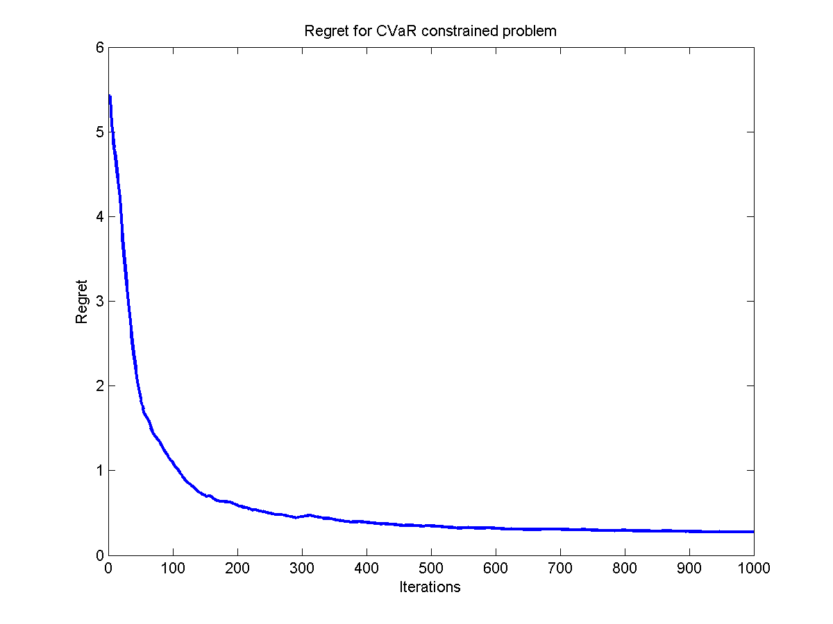
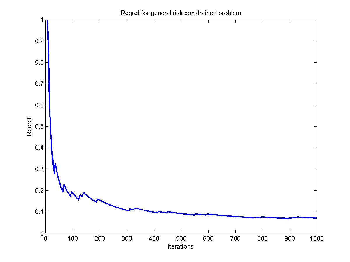
Figure 1: Regret for CVaR and general risk constrained problem

Here we conduct numerical experiments seeking compare the practical probability bounds for offline risk ranking by simulation and theoretical bounds provided by Theorem 5.4. We conduct the online risk ranking with Conditional value-at-risk as risk measure for 8 random variables follow $X\sim N(100,\,50)$ with target respectively as $\tau=115,\,117,\,119,\,121,\,123,\,125,\,127,\,129$. The following figure shows the relationship between the validation probability of ranking results with the iteration number. The maximum possible inversion number for this ranking system is $C_{8}^{2}=28$. The experiments are conducted under the case when inversion number $e$ equals $5,\,10,\,15,\,20$ and $25$ respectively. The $\delta$ equal $0.05$ for all the cases. Figure 3 shows that the practical bound attained by simulation is lower bound by the theoretical bounds derive in Theorem 5.4, thus the practical bound could serve as a conservative guidance on determined the required size of the sample to ensure a high probability of risk ranking validation.

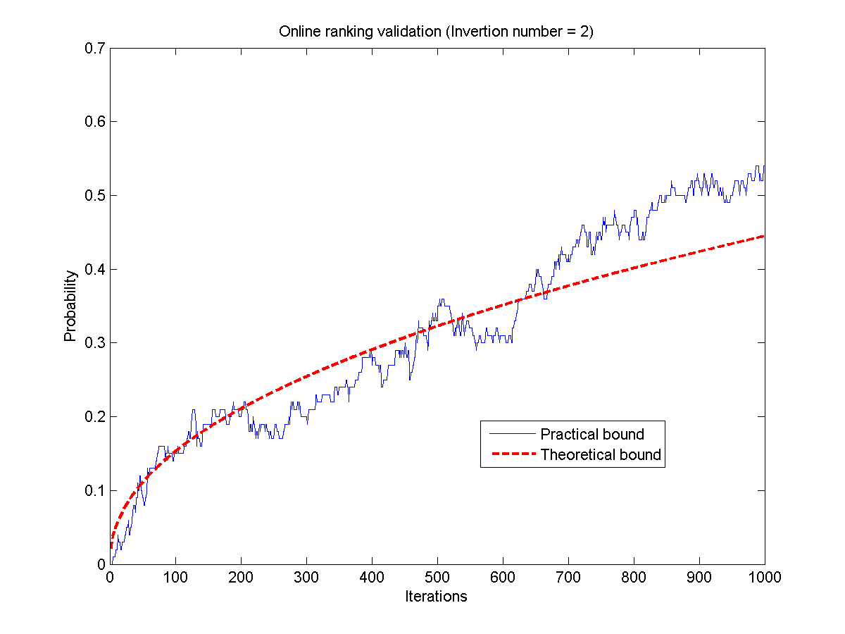
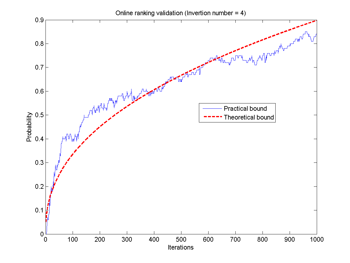
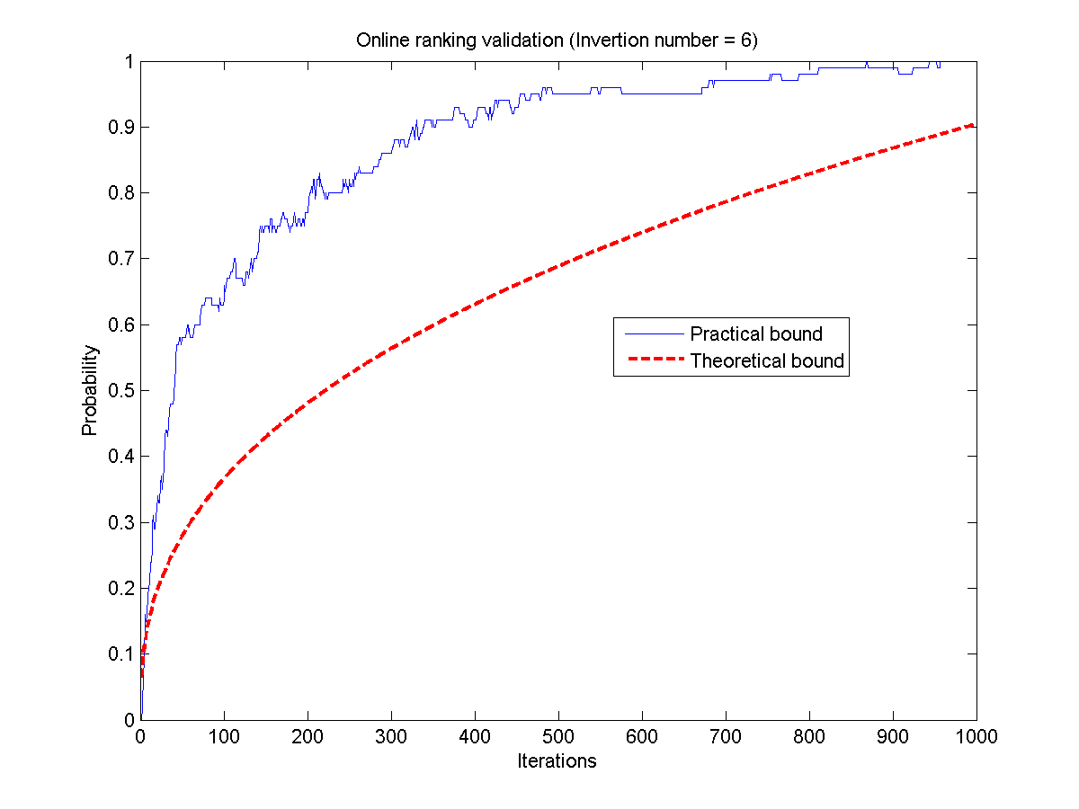
Figure 2: Online ranking validation

6.3 Risk assessment and ranking results

The following figure reveals the real-time risk assessment and ranking results with 1000 iterations of streaming concentration data of 13 EOCs. Here we use the Conditional value-at-risk as risk measure. From Figure 3, we can conclude that the Estrone, BPA, Triclosan, and Fipronil are among the most risky EOCs, and Salicylic acid, Sulpiride and Naproxen are among the least risky EOC. The risk level of other EOCs are intermediate. Starting from around 800 iterations, our ranking results becomes stable.

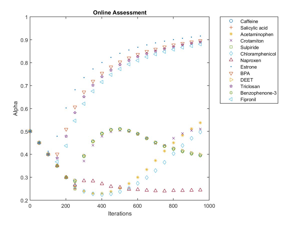
Figure 3: Online assessment and ranking result for EOCs

The following table shows the comparison online learning method and batch learning method. We observe that our online and offline computational methods produce similar ranking and assessment results, when online ranking is more sensitive compared to offline ranking, which will contribute more in capture the silent difference between the risk level of EOCs.

Contaminant	$\alpha$-offline	ranking-offline	$\alpha$-online	ranking-online
Caffeine	6.1035e-05	7	0.3897	9
Salicylic acid	0.0000	11	0.0000	12
Acetaminophen	0.5308	5	0.5598	5
Crotamiton	6.1035e-05	7	0.5106	7
Sulpiride	0.0000	11	0.0000	12
Chloramphenicol	0.3050	6	0.5221	6
Naproxen	6.1035e-05	7	0.2455	11
Estrone	0.7189	1	0.9202	1
BPA	0.7189	1	0.9014	2
DEET	6.1035e-05	7	0.3910	8
Triclosan	0.7189	1	0.8952	3
Benzophenone-3	6.1035e-05	7	0.3869	10
Fipronil	0.7189	1	0.8860	4

Table 3: Comparison of offline and online assessment and ranking

7 Conclusion

This paper proposes an risk assessment and ranking approach based on satisficing measure, and develops real-time risk assessment and ranking policy with online learning and optimization technique. The basic model is a satisficing optimization model with a family of risk constrained (Conditional value-at-risk or Optimized certainty equivalent). In the offline case, we consider performing risk assessment and ranking when we know the probability distribution of random outcomes or we have no known information about the probability distribution but have samples extracted from the underlying distribution in hand. Sample average approximation can attack both cases. We figure out the convergence rate with sample size and prove the validation of ranking result from approximated problem under offline case. For online stochastic optimization case, we develop an online primal-dual algorithm to solve the problem with a desired regret bound. For both offline and online case, we argue the minimal sample size or iteration times required to ensure a high probability that the estimated ranking is the same as the true ranking, as well as, given a certain sample size or iteration times, the probability that the loss function is bounded by a given benchmark.

Appendix I

Name	$\phi(t)\quad t\geq 0$	$\phi^{*}(s)$
Kullback-Leibler	$t\log t-t+1$	$\exp(s)-1$
Burg entropy	$-\log t+t-1$	$-\log(1-s),\quad s<1$
$\chi^{2}$distance	$\frac{1}{t}(t-1)^{2}$	$2-2\sqrt{1-s},\quad s<1$
Modified$\chi^{2}$distance	$(t-1)^{2}$	$\begin{cases}-1&\quad s<-2\\ s+s^{2}/4&\quad s\geq-2\end{cases}$
Hellinger distance	$(\sqrt{t}-1)^{2}$	$\frac{s}{1-s},\quad s<1$
$\chi$- divergence	$|t-1|^{\theta}$	$s+(\theta+1)\left(\frac{|s|}{\theta}\right)^{\theta/(\theta-1)}$
Variation distance	$|t-1|$	$\max\left\{-1,\,s\right\},\quad s\leq 1$
Cressie-Read	$\frac{1-\theta+\theta t-t^{\theta}}{\theta(1-\theta)},\quad t\neq 0,1$	$\frac{1}{\theta}(1-s(1-\theta))^{\theta/(1-\theta)}-\frac{1}{\theta},\quad s<\frac{1}{1-\theta}$

Table 4: Examples of $\phi-$divergence functions and their convex conjugate functions

Appendix II

Proof of Theorem 4.6: Problem (4) can be reformulated as

$$\max_{0\leq\alpha\leq 1,\,\eta\in\mathbb{R}} \left\{1-\alpha:\,g(\alpha):=\mathbb{E}^{P}\left[G\left(\alpha,\,\eta,\,X\right)\right]\leq\tau\right\},$$

and Problem (7) can be reformulated as

$$\max_{0\leq\alpha\leq 1,\,\eta\in\mathbb{R}} \left\{1-\alpha:\,g_{N}(\alpha):=\frac{1}{N}\sum_{n=1}^{N}G\left(\alpha,\,\eta,\,d_{n}\right)\leq\tau\right\},$$

Given $\epsilon>0$ define

$$X^{\epsilon}:=\left\{\alpha\in\left[0,\,1\right]:\,g(\alpha)\leq\tau+\epsilon\right\}.$$

Then $X^{0}$ represents the feasible region of Problem (4), and correspondingly we define

$$X_{N}^{\epsilon}:=\left\{\alpha\in\left[0,\,1\right]:\,g_{N}(\alpha)\leq\tau+\epsilon\right\}.$$

Our goal is to estimate $\mathbb{P}\left\{X^{-\epsilon}\subseteq X_{N}^{0}\subseteq X^{\epsilon}\right\}.$ That is, we want to claim a feasible solution of SAA of Problem (7) is $\epsilon-$feasible to the true problem. Suppose Assumption 4.1 hold. Given $\epsilon>0,$ we could set $v:=\left\{4(\Psi+\Phi)/\epsilon+2\right\}^{-1}$, and obtain

$$\mathbb{P}\left\{X^{-\epsilon}\subseteq X_{N}^{0}\subseteq X^{\epsilon}\right\}$$

$$\geq \mathbb{P}\left\{\exists\alpha\in(0,\,1],\,\textrm{s.t.}\,\Bigl{|}g_{N}(\alpha)-g(\alpha)\Bigr{|}\leq\epsilon\right\}$$

$$\geq 1-\mathbb{P}\left\{\exists\alpha\in(0,\,1],\,\textrm{s.t.}\,\sup_{\eta\in\mathbb{R}}\left\{\biggl{|}\mathbb{E}^{P}\left[\frac{1}{\alpha}\phi^{\ast}\left(X-\eta\right)\right]-\frac{1}{N}\sum_{n=1}^{N}\frac{1}{\alpha}\phi^{\ast}\left(d_{n}-\eta\right)\biggr{|}\right\}\geq\epsilon\right\}$$

$$\geq 1-\mathbb{P}\left\{\exists\alpha\in(0,\,1]_{v},\,\textrm{s.t.}\,\sup_{\eta\in E_{v}}\mathbb{E}^{P}\left[\frac{1}{\alpha}\phi^{\ast}\left(X-\eta\right)\right]-\frac{1}{N}\sum_{n=1}^{N}\frac{1}{\alpha}\phi^{\ast}\left(d_{n}-\eta\right)\geq\epsilon-(\Psi+\Psi_{N}+\Phi+\Phi_{N})v\right\}$$

$$-\mathbb{P}\left\{\exists\alpha\in(0,\,1]_{v},\,\textrm{s.t.}\,\sup_{\eta\in E_{v}}\frac{1}{N}\sum_{n=1}^{N}\frac{1}{\alpha}\phi^{\ast}\left(d_{n}-\eta\right)-\mathbb{E}^{P}\left[\frac{1}{\alpha}\phi^{\ast}\left(X-\eta\right)\right]\geq\epsilon-(\Psi+\Psi_{N}+\Phi+\Phi_{N})v\right\},$$

Then we have

$$\mathbb{P}\left\{X^{-\epsilon}\subseteq X_{N}^{0}\subseteq X^{\epsilon}\right\}$$

$$\geq 1-2\mathbb{P}\left\{\Psi_{N}>\Psi+\epsilon/2\right\}-2\mathbb{P}\left\{\Phi_{N}>\Phi+\epsilon/2\right\}$$

$$-2\sum_{\alpha\in(0,\,1],\,\eta\in E_{v}}\mathbb{P}\left\{\biggl{|}\mathbb{E}^{P}\left[\frac{1}{\alpha}\phi^{\ast}\left(X-\eta\right)\right]-\frac{1}{N}\sum_{n=1}^{N}\frac{1}{\alpha}\phi^{\ast}\left(d_{n}-\eta\right)\biggr{|}\geq\epsilon/2\right\}$$

$$\geq 1-2\exp\left\{-N\cdot b(\epsilon)\right\}-\sum_{\alpha\in(0,\,1],\,\eta\in E_{v}}\left[\exp\left\{-N\cdot b(\epsilon)\right\}\right]$$

$$\geq 1-2\left(2+\frac{D_{E}}{v^{2}}\right)\exp\left\{-N\cdot b(\epsilon)\right\},$$

where $b(\epsilon)\,:=\min_{\eta\in E_{v}}\left\{I_{\psi}(\Psi+\epsilon/2),\,I_{\phi}(\Phi+\epsilon/2),\,I_{\eta}(\epsilon/2),\,I_{\eta}(-\epsilon/2)\right\}$, and we have

$$b(\epsilon) \geq\min_{\alpha\in(0,1],\,\eta\in E_{v}}\left\{\frac{\epsilon^{2}}{8\textrm{VaR}\left[\phi(X)\right]},\,\frac{\epsilon^{2}}{8\textrm{VaR}\left[\psi(X)\right]},\,\frac{\epsilon^{2}}{\textrm{VaR}\left[G(\alpha,\,\eta,\,X)-\mathbb{E}\left[G(\alpha,\,\eta,\,X)\right]\right]}\right\}$$

$$\geq\frac{\epsilon^{2}}{8\sigma^{2}}.$$

Assume that there exists a positive number $C$ so that, $\tilde{\pi}\leq C$ uniformly, and $\epsilon_{0}$ that $\|\tau-\tilde{\tau}\|_{2}\leq\epsilon_{0}$. Given $0<\epsilon\leq c,$ we set $v:=\left\{4(\Psi+\Phi)C/(\epsilon-C\epsilon_{0})+2\right\}^{-1}$. It follows that

$$\mathbb{P}\left\{|\tilde{\alpha}-\alpha|\leq\epsilon\right\}$$

$$= \mathbb{P}\left\{|1-\tilde{\alpha}-(1-\alpha)|\leq\epsilon\right\}$$

$$\geq \mathbb{P}\left\{\biggl{|}\sup_{0\leq\alpha\leq 1,\,t\in C}\left\{1-\alpha+\tilde{\pi}\left[g_{N}(\alpha)-\tilde{\tau}\right]\right\}-\sup_{0\leq\alpha\leq 1,\,t\in C}\left\{1-\alpha+\tilde{\pi}\left[g(\alpha)-\tau\right]\right\}\biggr{|}\leq\epsilon\right\}$$

$$= \mathbb{P}\left\{\sup_{0\leq\alpha\leq 1}\biggl{|}\tilde{\pi}\left[g_{N}(\alpha)-g(\alpha)\right]\biggr{|}+|\tilde{\pi}\left(\tau-\tilde{\tau}\right)|\leq\epsilon\right\}$$

$$= \mathbb{P}\left\{\tilde{\pi}\left[\sup_{0\leq\alpha\leq 1}\biggl{|}g_{N}(\alpha)-g(\alpha)\biggr{|}+|\tau-\tilde{\tau}|\right]\leq\epsilon\right\}$$

$$\geq \mathbb{P}\left\{\sup_{0\leq\alpha\leq 1}\biggl{|}g_{N}(\alpha)-g(\alpha)\biggr{|}\leq\frac{\epsilon}{C}-\epsilon_{0}\right\}$$

$$= 1-\mathbb{P}\left\{\sup_{0\leq\alpha\leq 1}\biggl{|}g_{N}(\alpha)-g(\alpha)\biggr{|}\geq\frac{\epsilon}{C}-\epsilon_{0}\right\}$$

$$\geq 1-\mathbb{P}\left\{\exists 0\leq\alpha\leq 1\,\textrm{s.t.}\,g_{N}(\alpha)-g(\alpha)>\frac{\epsilon}{C}-\epsilon_{0}\right\}$$

$$-\mathbb{P}\left\{\exists 0\leq\alpha\leq 1,\,\textrm{s.t.}\,g_{N}(\alpha)-g(\alpha)<-\frac{\epsilon}{C}+\epsilon_{0}\right\}$$

$$\geq \mathbb{P}\left\{|\tilde{\alpha}-\alpha|\leq\epsilon\right\}\geq 1-2\left(2+\frac{D_{E}}{v^{2}}\right)\exp\left(-\frac{N(\epsilon-C\epsilon_{0})^{2}}{8\sigma^{2}C^{2}}\right),$$

where

$$v:=\left\{4(\Psi+\Phi)C/(\epsilon-C\epsilon_{0})+2\right\}^{-1},$$

and

$$\sigma^{2}:=\text{$\max$}_{\alpha\in(0,1],\,\eta\in E}\left\{\textrm{VaR}\left[\phi(X)\right],\,\textrm{VaR}\left[\psi(X)\right],\,\textrm{VaR}\left[G(\alpha,\,\eta,\,X)-\mathbb{E}\left[G(\alpha,\,\eta,\,X)\right]\right]\right\}.$$

In addition, we have

$$\mathbb{P}\left\{|\tilde{l}_{L}-(1-\alpha)|\leq c-\epsilon\right\}$$

$$= \mathbb{P}\left\{|\widetilde{l}-z_{\gamma/2}S_{\tilde{l}}-(1-\alpha)|\leq c-\epsilon\right\}$$

$$\geq \mathbb{P}\left\{\Biggl{|}\frac{1}{M_{l}}\sum_{m=1}^{M_{l}}\inf_{\alpha\in(0,\,1]}\tilde{\pi}\left[\sup_{u\geq 0,\,\eta\in\mathbb{R}}N_{u}^{-1}\sum_{n=1}^{N_{u}}\left\{\eta+u\mu+\frac{u}{\alpha}\phi^{*}\left(\frac{d_{n}^{m}-\eta}{u}\right)\right\}-\tau\right]\Biggr{|}+|z_{\gamma/2}S_{\tilde{l}}|\leq c-\epsilon\right\}$$

$$\geq \mathbb{P}\left\{\tilde{\pi}\sup_{\alpha\in\left[0,\,1\right]}\biggl{|}g_{N}(\alpha)-g(\alpha)\biggr{|}+|z_{\gamma/2}S_{\tilde{l}}|\leq c-\epsilon\right\}$$

$$\geq \mathbb{P}\left\{\tilde{\pi}\sup_{\alpha\in\left[0,\,1\right]}\biggl{|}g_{N}(\alpha)-g(\alpha)\biggr{|}\leq c-\epsilon-z_{\gamma/2}\cdot\frac{M^{2}}{4}\right\}$$

$$\geq 1-2\left(2+\frac{D_{E}}{v^{2}}\right)\exp\left\{\frac{-N\cdot(c-\epsilon-z_{\gamma/2}\cdot\frac{M^{2}}{4})^{2}}{8\sigma^{2}}\right\},$$

where

$$v:=\left\{4(\Psi+\Phi)/(c-\epsilon-z_{\gamma/2}\cdot\frac{M^{2}}{4})+2\right\}^{-1},$$

and

$$\sigma^{2}:=\text{$\max$}_{\alpha\in(0,1],\,\eta\in E}\left\{\textrm{VaR}\left[\phi(X)\right],\,\textrm{VaR}\left[\psi(X)\right],\,\textrm{VaR}\left[G(\alpha,\,\eta,\,X)-\mathbb{E}\left[G(\alpha,\,\eta,\,X)\right]\right]\right\}.$$

Based on above arguments, next we study the relationship between the sample size and the validation probability of ranking by SAA problem to the original problem.

Appendix III

Proof of Theorem 5.3: In this section, we will prove Theorem 5.3. Denote $A_{t}:=\frac{1}{2}\|\alpha_{t}-\alpha^{\ast}\|_{2}^{2}$ . We can write

$$A_{t}= \frac{1}{2}\|\text{$\prod$}_{(0,\,1]}\left(\alpha_{t-1}-\frac{G(\alpha_{t-1},\,\eta_{t-1},\,\lambda_{t-1})}{t}\right)-\alpha^{\ast}\|_{2}^{2}$$

$$\leq \frac{1}{2}\|\alpha_{t-1}-\frac{G(\alpha_{t-1},\,\eta_{t-1},\,\lambda_{t-1})}{t}-\alpha^{\ast}\|_{2}^{2}$$

$$= A_{t}+\frac{1}{2t^{2}}\|G(\alpha_{t-1},\,\eta_{t-1},\,\lambda_{t-1})\|_{2}^{2}$$

$$+\frac{1}{t}(\alpha_{t-1}-\alpha^{\ast})^{\top}G(\alpha_{t-1},\,\eta_{t-1},\,\lambda_{t-1},)$$

and we also have

$$\mathbb{E}\left[(\alpha_{t-1}-\alpha^{\ast})^{\top}G(\alpha_{t-1},\,\eta_{t-1},\,\lambda_{t-1})\right]$$

$$=\mathbb{E}_{d_{t-2}}\left\{\mathbb{E}_{d_{t-1}}\left[(\alpha_{t-1}-\alpha^{\ast})^{\top}G(\alpha_{t-1},\,\eta_{t-1},\,\lambda_{t-1})\right]\right\}$$

$$=\mathbb{E}_{d_{t-2}}\left\{(\alpha_{t-1}-\alpha^{\ast})^{\top}\mathbb{E}\left[G(\alpha_{t-1},\,\eta_{t-1},\,\lambda_{t-1})\right]\right\}$$

$$=\mathbb{E}\left[(\alpha_{t-1}-\alpha^{\ast})^{\top}g(\alpha_{t-1},\,\eta_{t-1},\,\lambda_{t-1})\right].$$

By taking the expectation of both side, we obtain

$$\frac{1}{2}\mathbb{E}\left[\|\alpha_{t}-\alpha^{\ast}\|_{2}^{2}\right]\leq\frac{1}{2}\mathbb{E}\left[\|\alpha_{t-1}-\alpha^{\ast}\|_{2}^{2}\right]+\frac{1}{t}\mathbb{E}\left[(\alpha_{t-1}-\alpha^{\ast})^{\top}g(\alpha_{t},\,\eta_{t},\,\lambda_{t})\right]+\frac{1}{2t^{2}}M^{2},$$

where, based on Assumption 5.2 (i), obtain

$$M^{2}:=\sup_{(\alpha,\,\eta)\in(0,1],\,\lambda\leq 0}\mathbb{E}\left[\|G(\alpha_{t-1},\,\eta_{t-1},\,\lambda_{t-1})\|_{2}^{2}\right].$$

By Lipschitz continuous of function $g$ summarized in Assumption 5.2 (ii), we have

$$\mathbb{E}\left[(\alpha_{t}-\alpha^{\ast})^{\top}g(\alpha_{t},\,\eta_{t},\,\lambda_{t})\right]\geq\mathbb{E}\left[(\alpha_{t}-\alpha^{\ast})^{\top}\left(g(\alpha_{t},\,\eta_{t},\,\lambda_{t})-g(\alpha^{\ast},\,\eta_{t},\,\lambda_{t})\right)\right]\geq L_{g}\mathbb{E}\left[\|\alpha_{t}-\alpha^{\ast}\|_{2}^{2}\right].$$

Therefore it follows that

$$\mathbb{E}\left[\|\alpha_{t}-\alpha^{\ast}\|_{2}^{2}\right]\leq(1-2L_{g}/t)\mathbb{E}\left[\|\alpha_{t-1}-\alpha^{\ast}\|_{2}^{2}\right]+M^{2}/t^{2},$$

and by induction we get the deterministic convergence rate

$$\mathbb{E}\left[\|\alpha_{t}-\alpha^{\ast}\|_{2}^{2}\right]\leq\kappa/t,$$

where

$$\kappa:=\max\left\{M^{2}/(2L_{g}-1)^{-1},\,\|\alpha^{0}-\alpha^{\ast}\|_{2}^{2}\right\}.$$

Follow the same idea ,we obtain

$$\mathbb{E}\left[\|\alpha_{t}-\alpha^{\ast}\|_{2}^{2}+\|\eta_{t}-\eta^{\ast}\|_{2}^{2}+\|\lambda_{t}-\lambda^{\ast}\|_{2}^{2}\right]\leq 3\kappa/t,$$

where

$$\kappa:=\max\left\{M^{2}/(2L_{g}-1)^{-1},\,\|\alpha_{0}-\alpha^{\ast}\|_{2}^{2},\,\|\eta_{0}-\eta^{\ast}\|_{2}^{2},\,\|\lambda_{0}-\lambda^{\ast}\|_{2}^{2}\right\},$$

Let $\delta_{t}=\left[L(\alpha^{\ast},\,\eta^{\ast},\,\lambda^{\ast})\right](d_{t})-C^{\ast}$ and $\xi_{t}=\left[L(\alpha_{t-1},\,\eta_{t-1},\,\lambda_{t-1})\right](d_{t})-\left[L(\alpha^{\ast},\,\eta^{\ast},\,\lambda^{\ast})\right](d_{t})$ be the statistical error and approximation error, where $\alpha^{\ast},\,\eta^{\ast},\,\lambda^{\ast}$ denote the optimal primal and dual solution for problem 8. Therefore the step 4 in Algorithm 2 is equivalent to

$$C_{t}=C_{t-1}-\frac{1}{t}\left(C_{t-1}-C^{\ast}+\xi_{t}+\delta_{t}\right).$$

Expanding, we have following inequalities

$$\|C_{t}-C^{\ast}\|_{2}^{2} \leq\|C_{t-1}-C^{\ast}\|_{2}^{2}+\|\frac{1}{t}\left(C_{t-1}-C^{\ast}+\xi_{t}+\delta_{t}\right)\|_{2}^{2}$$

$$-2(C_{t-1}-C^{\ast})^{\top}\frac{1}{t}\left(C_{t-1}-C^{\ast}+\xi_{t}+\delta_{t}\right),$$

$$\mathbb{E}\left[C_{t-1}-\left[L(\alpha_{t-1},\,\eta_{t-1},\,\lambda_{t-1})\right](d_{t})\right]^{2}\leq B,$$

$$\|C_{t}-C^{\ast}\|_{2}^{2}\leq\|C_{t-1}-C^{\ast}\|_{2}^{2}+\frac{B-2}{t^{2}}-\frac{2}{t}\kappa_{0}\|C_{t-1}-C^{\ast}\|_{2}^{2}-\frac{L_{\Phi}}{t\kappa_{0}}\left(\|\alpha_{t}-\alpha^{\ast}\|_{2}^{2}+\|\eta_{t}-\eta^{\ast}\|_{2}^{2}+\|\lambda_{t}-\lambda^{\ast}\|_{2}^{2}\right),$$

and

$$\|C_{t}-C^{\ast}\|_{2}^{2}\leq(1-2\kappa_{0}/t)\|C_{t-1}-C^{\ast}\|_{2}^{2}+\frac{B-2-\frac{3\kappa L_{\Phi}}{\kappa_{0}}}{t^{2}}.$$

Then we have

$$\mathbb{E}\left[\|C_{t}-C^{\ast}\|_{2}^{2}\right]\leq\kappa^{\prime}/t,$$

where

$$\kappa^{\prime}:=\max\left\{B-2-\frac{3\kappa L_{\Phi}}{\kappa_{0}}/(2\kappa_{0}-1)^{-1},\,\|C_{0}-C^{\ast}\|_{2}^{2}\right\},$$

Thus we get the desired result.

References

- Armbruster and Delage, (2015) Armbruster, B. and Delage, E. (2015). Decision making under uncertainty when preference information is incomplete. Management Science, 61(1):111–128.
- Artzner et al., (1999) Artzner, P., Delbaen, F., Eber, J.-M., and Heath, D. (1999). Coherent measures of risk. Mathematical finance, 9(3):203–228.
- Bardou et al., (2009) Bardou, O., Frikha, N., and Pages, G. (2009). Computing var and cvar using stochastic approximation and adaptive unconstrained importance sampling. Monte Carlo Methods and Applications, 15(3):173–210.
- Ben-Tal and Teboulle, (1986) Ben-Tal, A. and Teboulle, M. (1986). Expected utility, penalty functions, and duality in stochastic nonlinear programming. Management Science, 32(11):1445–1466.
- Ben-Tal and Teboulle, (2007) Ben-Tal, A. and Teboulle, M. (2007). An old-new concept of convex risk measures: The optimized certainty equivalent. Mathematical Finance, 17(3):449–476.
- Boyd and Vandenberghe, (2004) Boyd, S. and Vandenberghe, L. (2004). Convex optimization. Cambridge university press.
- Bradley and Terry, (1952) Bradley, R. A. and Terry, M. E. (1952). Rank analysis of incomplete block designs the method of paired comparisons. Biometrika, 39(3-4):324–345.
- Brown et al., (2006) Brown, D. B. et al. (2006). Risk and robust optimization. PhD thesis, Massachusetts Institute of Technology.
- Brown et al., (2012) Brown, D. B., Giorgi, E. D., and Sim, M. (2012). Aspirational preferences and their representation by risk measures. Management Science, 58(11):2095–2113.
- Brown and Sim, (2009) Brown, D. B. and Sim, M. (2009). Satisficing measures for analysis of risky positions. Management Science, 55(1):71–84.
- Bubeck, (2011) Bubeck, S. (2011). Introduction to online optimization. Lecture Notes.
- Carbonetto et al., (2009) Carbonetto, P., Schmidt, M., and Freitas, N. D. (2009). An interior-point stochastic approximation method and an l1-regularized delta rule. In Advances in neural information processing systems, pages 233–240.
- Chen, (2012) Chen, H. (2012). The convergence rate of a regularized ranking algorithm. Journal of Approximation Theory, 164(12):1513–1519.
- Chen et al., (2013) Chen, H., Tang, Y., Li, L., Yuan, Y., Li, X., and Tang, Y. (2013). Error analysis of stochastic gradient descent ranking. IEEE transactions on cybernetics, 43(3):898–909.
- Chen et al., (2014) Chen, L. G., Long, D. Z., and Perakis, G. (2014). The impact of a target on newsvendor decisions. Manufacturing & Service Operations Management, 17(1):78–86.
- Dai et al., (2016) Dai, Z., Li, D., and Wen, F. (2016). Worse-case conditional value-at-risk for asymmetrically distributed asset scenarios returns. Journal of Computational Analysis & Applications, 20(1).
- De Giorgi and Post, (2011) De Giorgi, E. G. and Post, T. (2011). Loss aversion with a state-dependent reference point. Management Science, 57(6):1094–1110.
- Delage and Li, (2015) Delage, E. and Li, J. Y. (2015). Minimizing risk exposure when the choice of a risk measure is ambiguous. Technical report, Tech. rep., Les Cahiers du GERAD G–2015–05.
- Delage and Ye, (2010) Delage, E. and Ye, Y. (2010). Distributionally robust optimization under moment uncertainty with application to data-driven problems. Operations research, 58(3):595–612.
- Duchi et al., (2011) Duchi, J., Hazan, E., and Singer, Y. (2011). Adaptive subgradient methods for online learning and stochastic optimization. Journal of Machine Learning Research, 12(Jul):2121–2159.
- Föllmer and Knispel, (2013) Föllmer, H. and Knispel, T. (2013). Convex risk measures: Basic facts, law-invariance and beyond, asymptotics for large portfolios. Handbook of the Fundamentals of Financial Decision Making, Part II, pages 507–554.
- Föllmer and Schied, (2011) Föllmer, H. and Schied, A. (2011). Stochastic finance: an introduction in discrete time. Walter de Gruyter.
- Frey, (2007) Frey, J. C. (2007). New imperfect rankings models for ranked set sampling. Journal of Statistical planning and Inference, 137(4):1433–1445.
- Ghahramani, (2001) Ghahramani, Z. (2001). An introduction to hidden markov models and bayesian networks. International Journal of Pattern Recognition and Artificial Intelligence, 15(01):9–42.
- Haslum and Årnes, (2006) Haslum, K. and Årnes, A. (2006). Multisensor real-time risk assessment using continuous-time hidden markov models. In Computational Intelligence and Security, 2006 International Conference on, volume 2, pages 1536–1540. IEEE.
- Homem-De-Mello, (2003) Homem-De-Mello, T. (2003). Variable-sample methods for stochastic optimization. ACM Transactions on Modeling and Computer Simulation (TOMACS), 13(2):108–133.
- Hu et al., (2012) Hu, J., Homem-de Mello, T., and Mehrotra, S. (2012). Sample average approximation of stochastic dominance constrained programs. Mathematical programming, 133(1-2):171–201.
- Jiang et al., (2015) Jiang, G., Fu, M. C., and Xu, C. (2015). Optimal importance sampling for simulation of lévy processes. In Proceedings of the 2015 Winter Simulation Conference, pages 3813–3824. IEEE Press.
- Kiefer et al., (1952) Kiefer, J., Wolfowitz, J., et al. (1952). Stochastic estimation of the maximum of a regression function. The Annals of Mathematical Statistics, 23(3):462–466.
- Kim et al., (2015) Kim, S., Pasupathy, R., and Henderson, S. G. (2015). A guide to sample average approximation. In Handbook of simulation optimization, pages 207–243. Springer.
- Kőszegi and Rabin, (2006) Kőszegi, B. and Rabin, M. (2006). A model of reference-dependent preferences. The Quarterly Journal of Economics, pages 1133–1165.
- Kriukova et al., (2016) Kriukova, G., Pereverzyev, S. V., and Tkachenko, P. (2016). On the convergence rate and some applications of regularized ranking algorithms. Journal of Complexity, 33:14–29.
- Krokhmal et al., (2002) Krokhmal, P., Palmquist, J., and Uryasev, S. (2002). Portfolio optimization with conditional value-at-risk objective and constraints. Journal of risk, 4:43–68.
- Kushner and Yin, (2003) Kushner, H. and Yin, G. G. (2003). Stochastic approximation and recursive algorithms and applications, volume 35. Springer Science & Business Media.
- Li and Guo, (2009) Li, W. and Guo, Z. (2009). Hidden markov model based real time network security quantification method. In Networks Security, Wireless Communications and Trusted Computing, 2009. NSWCTC’09. International Conference on, volume 2, pages 94–100. IEEE.
- Liu et al., (2017) Liu, Y., Li, Y., and Hu, L. (2017). Departure time and route choices in bottleneck equilibrium under risk and ambiguity. Transportation Research Part B: Methodological.
- Luce, (2005) Luce, R. D. (2005). Individual choice behavior: A theoretical analysis. Courier Corporation.
- Mahdavi et al., (2012) Mahdavi, M., Yang, T., and Jin, R. (2012). Online stochastic optimization with multiple objectives. arXiv preprint arXiv:1211.6013.
- Noyan and Rudolf, (2013) Noyan, N. and Rudolf, G. (2013). Optimization with multivariate conditional value-at-risk constraints. Operations Research, 61(4):990–1013.
- Pal et al., (2014) Pal, A., He, Y., Jekel, M., Reinhard, M., and Gin, K. Y.-H. (2014). Emerging contaminants of public health significance as water quality indicator compounds in the urban water cycle. Environment international, 71:46–62.
- Paltrinieri et al., (2014) Paltrinieri, N., Khan, F., Amyotte, P., and Cozzani, V. (2014). Dynamic approach to risk management: application to the hoeganaes metal dust accidents. Process Safety and Environmental Protection, 92(6):669–679.
- Postek et al., (2015) Postek, K., Den Hertog, D., and Melenberg, B. (2015). Computationally tractable counterparts of distributionally robust constraints on risk measures.
- Robbins and Monro, (1951) Robbins, H. and Monro, S. (1951). A stochastic approximation method. The annals of mathematical statistics, pages 400–407.
- Rockafellar and Uryasev, (2000) Rockafellar, R. T. and Uryasev, S. (2000). Optimization of conditional value-at-risk. Journal of risk, 2:21–42.
- Rockafellar and Uryasev, (2013) Rockafellar, R. T. and Uryasev, S. (2013). The fundamental risk quadrangle in risk management, optimization and statistical estimation. Surveys in Operations Research and Management Science, 18(1):33–53.
- Ruszczynski and Shapiro, (2006) Ruszczynski, A. and Shapiro, A. (2006). Optimization of convex risk functions. Mathematics of operations research, 31(3):433–452.
- Sandoy and Aven, (2006) Sandoy, M. and Aven, T. (2006). Real time updating of risk assessments during a drilling operation-alternative bayesian approaches. International journal of reliability, quality and safety engineering, 13(1):85–95.
- Shalev, (2000) Shalev, J. (2000). Loss aversion equilibrium. International Journal of Game Theory, 29(2):269–287.
- Shalev-Shwartz, (2011) Shalev-Shwartz, S. (2011). Online learning and online convex optimization. Foundations and Trends in Machine Learning, 4(2):107–194.
- Shapiro, (2013) Shapiro, A. (2013). On kusuoka representation of law invariant risk measures. Mathematics of Operations Research, 38(1):142–152.
- Simon, (1955) Simon, H. A. (1955). A behavioral model of rational choice. The quarterly journal of economics, pages 99–118.
- Simon, (1959) Simon, H. A. (1959). Theories of decision-making in economics and behavioral science. The American economic review, 49(3):253–283.
- Sugden, (2003) Sugden, R. (2003). Reference-dependent subjective expected utility. Journal of economic theory, 111(2):172–191.
- Tan et al., (2008) Tan, X., Zhang, Y., Cui, X., and Xi, H. (2008). Using hidden markov models to evaluate the real-time risks of network. In Knowledge Acquisition and Modeling Workshop, 2008. KAM Workshop 2008. IEEE International Symposium on, pages 490–493. IEEE.
- Van Asselt et al., (2013) Van Asselt, E., van der Spiegel, M., Noordam, M., Pikkemaat, M., and van der Fels-Klerx, H. (2013). Risk ranking of chemical hazards in food: a case study on antibiotics in the netherlands. Food Research International, 54(2):1636–1642.
- Wang and Ahmed, (2008) Wang, W. and Ahmed, S. (2008). Sample average approximation of expected value constrained stochastic programs. Operations Research Letters, 36(5):515–519.
- Weng and Lin, (2011) Weng, R. C. and Lin, C.-J. (2011). A bayesian approximation method for online ranking. The Journal of Machine Learning Research, 12:267–300.
- Xu and Yu, (2014) Xu, L. and Yu, B. (2014). Cvar-constrained stochastic programming reformulation for stochastic nonlinear complementarity problems. Computational Optimization and Applications, 58(2):483–501.
- Yu-Ting et al., (2014) Yu-Ting, D., Hai-Peng, Q., and Xi-Long, T. (2014). Real-time risk assessment based on hidden markov model and security configuration. In Information Science, Electronics and Electrical Engineering (ISEEE), 2014 International Conference on, volume 3, pages 1600–1603. IEEE.
- Zhang and Wang, (2012) Zhang, C. and Wang, X. (2012). Health risk assessment of urban surface waters based on real-time pcr detection of typical pathogens. Human and Ecological Risk Assessment: An International Journal, 18(2):329–337.
- Zhang and Cao, (2012) Zhang, Y. and Cao, F. (2012). Analysis of convergence performance of neural networks ranking algorithm. Neural Networks, 34:65–71.