Helioseismic inversion to infer depth profile of solar meridional flow using spherical Born kernels

Abstract

Accurate inference of solar meridional flow is of crucial importance for the understanding of solar dynamo process. Wave travel times, as measured on the surface, will change if the waves encounter perturbations e.g. in the sound speed or flows, as they propagate through the solar interior. Using functions called sensitivity kernels, we may image the underlying anomalies that cause measured shifts in travel times. The inference of large-scale structures e.g meridional circulation requires computing sensitivity kernels in spherical geometry. Mandal et al. (2017) have computed such spherical kernels in the limit of the first-Born approximation. In this work, we perform an inversion for meridional circulation using travel-time measurements obtained from $6$ years of SDO/HMI data and those sensitivity kernels. We enforce mass conservation by inverting for a stream function. The number of free parameters is reduced by projecting the solution on to cubic B-splines in radius and derivatives of the Legendre-polynomial basis in latitude, thereby improving the condition number of the inverse problem. We validate our approach for synthetic observations before performing the actual inversion. The inversion suggests a single-cell profile with the return-flow occurring at depths below $0.78\,R_{\odot}$.

1 Introduction

Observation of solar meridional circulation is challenging because of its small magnitude compared to other flows at the solar surface. Improvements in observational techniques have made it feasible to reliably infer the profile of meridional circulation at the surface and near surface layers through a variety of techniques e.g., Doppler-shift measurement (Duvall, 1979; Hathaway et al., 1996; Ulrich, 2010), tracking of surface features e.g., small scale magnetic remnants (Komm et al., 1993; Hathaway, 2012), ring-diagram analysis (Schou & Bogart, 1998; Basu et al., 1999; Haber et al., 2002; González Hernández et al., 2008; Basu & Antia, 2010), time-distance helioseismology (Giles et al., 1997). All these studies show that the magnitude of meridional circulation at mid-latitudes in the near-surface region is 10–20 m s^-1 at mid-latitudes, depending on the phase of the solar cycle and is directed poleward in both hemispheres. Mass conservation requires there to be an equatorward return flow below the solar surface. The location of the return flow plays a crucial role in some models of the solar dynamo. There have been several attempts to understand the internal structure of meridional circulation using helioseismic techniques e.g., global helioseismology (Schad et al., 2013; Woodard et al., 2013), time-distance helioseismology (Zhao et al., 2013; Jackiewicz et al., 2015; Rajaguru & Antia, 2015; Böning et al., 2017; Chen & Zhao, 2017) etc. Such studies are very important to constrain dynamo models (Choudhuri et al., 1995; Dikpati et al., 2010) since meridional circulation is believed to carry magnetic field as well as transport energy and angular momentum in the convection zone.

These studies have arrived at a variety of conclusions. From the analysis of two years of continuous data taken by SDO/HMI, Zhao et al. (2013) reported multiple cells in depth with a return flow starting at about $0.9\>R_{\odot}$ and the second cell below $0.82\,R_{\odot}$. Using 2 years of GONG data, Jackiewicz et al. (2015) obtained results that agreed with Zhao et al. (2013) about the shallow return flow but could not find the second cell in the deeper convection zone. Recently, Chen & Zhao (2017) using $7$ years of SDO/HMI data covering $2010$ May 1 to $2017$ April $30$ found qualitatively similar profile as Zhao et al. (2013). These studies did not apply the mass conservation constraint. Using 4 years of HMI data, Rajaguru & Antia (2015) found a single-cell profile with return flow below $0.77\,R_{\odot}$ using stream functions which automatically ensures mass conservation. On the other hand, Schad et al. (2013) found multiple cells in both latitude and depth, which is very different from those found using time-distance helioseismology.

Systematics and noise significantly affect results obtained below $0.9\,R_{\odot}$ using time-distance helioseismology. All studies have considered data obtained from different instruments covering different periods of time. Sensitivity kernels computed using ray theory were used by (Zhao et al., 2013; Jackiewicz et al., 2015; Rajaguru & Antia, 2015; Chen & Zhao, 2017) to invert for flows. Ray kernels are sensitive only to perturbations along ray path. If the length scale of the perturbation is smaller than the acoustic wavelength, results using ray kernels may not be reliable (Birch et al., 2001; Birch & Felder, 2004).

The first-Born approximation, an alternative to ray theory, does not suffer from the above limitation. Recently, Mandal et al. (2017) computed travel-time sensitivity kernels in the Born limit in spherical geometry (two other alternative approaches were proposed independently by Böning et al., 2016; Gizon et al., 2017). Using Born kernels, Böning et al. (2017) inverted for meridional circulation and found return flow at $0.9\>R_{\odot}$ using a SOLA (Pijpers & Thompson, 1994) inversion technique. They found that both single and multiple-cell profiles are consistent with their measured travel times.

In this work, we use a stream-function approach, which automatically takes into account mass conservation and compute relevant sensitivity kernels. The other advantage of using stream functions is that both radial and latitudinal components of the meridional flow may be simultaneously derived from it.

2 Travel-time measurements

Helioseismic travel times capturing the signals due to meridional flows are estimated the same way as described in detail in Rajaguru & Antia (2015). The basic data used are the full-disk Doppler observations made by the Helioseismic and Magnetic Imager (HMI) onboard the Solar Dynamics Observatory (SDO), and we have added two more years of data to that of Rajaguru & Antia (2015) covering a total length of six years ($2010$ May $1$ through $2016$ April $30$). Each estimate of travel time is made from a Gabor wavelet (Kosovichev & Duvall, 1997) fit to the monthly average of time-distance correlations computed in point-to-point deep-focus arc geometry employing 60 travel distances. Travel distances ranging between $2.16^{\circ}$ and $44.64^{\circ}$in steps of $0.72^{\circ}$, covering depths from near the surface down to about $0.7\>R_{\odot}$. A major uncertainty in travel time estimates is the center-to-limb systematics - CLS (Zhao et al., 2012; Baldner & Schou, 2012; Rajaguru & Antia, 2015; Zhao et al., 2013) whose magnitude is several times of the signal due to meridional flows. We correct the N-S (or the meridional direction) travel times for this systematics in the same way as originally proposed by Zhao et al. (2012) and also as done by Rajaguru & Antia (2015): CLS is estimated from the antisymmetric component of W-E travel times (Figure 1) (the symmetric part corresponds to the solar rotation), which are then subtracted from the N-S travel times. These W-E travel times are estimated from the central W-E equatorial belt spanning 15 degrees on either side of the equator. Recently, Chen & Zhao (2017) have proposed a new empirical method to remove the systematics. They measure travel-time shifts between two points located on the solar disk for many different azimuthal angles and skip distances, followed by solving a system of linear equations containing both center-to-limb systematics and travel-time shifts due to meridional flow. In addition, Chen & Zhao (2017) have removed data pixels containing fields stronger than a threshold of $10$ G, following a method suggested by Liang & Chou (2015). In our travel-time measurement process, we have not removed the oscillation signals over the strongly magnetized surface regions. It should be noted that surface magnetic fields have been shown to corrupt the meridional flow measurements (Liang & Chou, 2015); although such influence of surface regions is not expected to majorly affect the overall inferences on the deep structure of meridional circulation inferred from 6 years of observations, a detailed analysis with and without the surface magnetic regions’ removal is necessary to quantify the surface effects. However, detailed analyses of the character of center-to-limb systematics and its dependence on the frequency of acoustic waves (Rajaguru and Antia 2018, work in progress, and Chen & Zhao, 2018) indicate that further careful study is needed to fully account for them in the current estimates of meridional flow travel times. Measured travel times induced by solar meridional flow from our analyses and corresponding errors have been shown in Figure. (2).

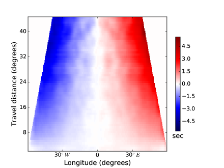
Figure 1: West minus east travel time, considered as center-to-limb systematics are plotted. These has been subtracted from north minus south travel time to obtain travel time shift due to solar meridional flow which are shown in the left panel of Figure 2.

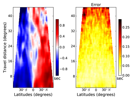
Figure 2: Left panel shows the measured travel times for solar meridional flow and right panel shows corresponding errors in the measurements. The travel time differences plotted are southward minus northward travel times, i.e. $\delta\tau=\tau_{\text{NS}}-\tau_{\text{SN}}$, where $\tau_{\text{NS}}$ is the travel time from north-arc to south-arc and $\tau_{\text{SN}}$ is that in the opposite direction.

3 forward modeling with spherical Born kernel

An efficient approach to compute sensitivity kernels in spherical geometry was proposed by Mandal et al. (2017). They showed that Green’s function can be expressed as (Equation 12 and 13 from Mandal et al., 2017)

$$G_{rr}(\mathbf{r},\mathbf{r}_{s},\omega) = \sum_{\ell}\frac{(2\ell+1)}{4\pi}\alpha_{\ell\omega}(r)P_{\ell}(\cos(\hat{\mathbf{r}}\cdot\hat{\mathbf{r}}_{s})),$$ (1)

$$\mathbf{G}_{hr}(\mathbf{r},\mathbf{r}_{s},\omega) = \sum_{\ell}\frac{(2\ell+1)}{4\pi\omega^{2}\rho_{0}}\beta_{\ell\omega}(r)\bm{\nabla}_{h}P_{\ell}(\cos(\hat{\mathbf{r}}\cdot\hat{\mathbf{r}}_{s})),$$ (2)

where $G_{rr}(\mathbf{r},\mathbf{r}_{s},\omega)$ and $\mathbf{G}_{hr}(\mathbf{r},\mathbf{r}_{s},\omega)=\left(G_{\theta r}\left(\mathbf{r},\mathbf{r}_{s},\omega\right),G_{\phi r}\left(\mathbf{r},\mathbf{r}_{s},\omega\right)\right)$ are radial and tangential components of the displacement of a wave with temporal frequency $\omega,$ measured at $\mathbf{r}$ due to a point source placed at $\mathbf{r}_{s}$, $P_{\ell}$ the Legendre polynomial of degree $\ell$. The terms $\alpha_{\ell\omega},\,\beta_{\ell\omega}$ are obtained by solving a coupled differential equation (Equation 10 in Mandal et al., 2017) using a finite-difference based scheme for each harmonic degree $\ell$ and frequency $\omega$. We compute the pair $\left(\alpha_{\ell\omega},\,\beta_{\ell\omega}\right)$ once and use them to evaluate Green’s function, which is used subsequently in obtaining kernels. The expression of sensitivity kernels for stream function, $K_{\psi}$, can be written in terms of Green’s function and its derivatives. The kernel computation time depends on the size of the $(r,\theta,\phi)$ grid used in the analysis, maximum harmonic degree for Green’s function computation and resolution in frequency. In this work, we consider $1398\times 200\times 400$ grid points spanning $0.7\,R_{\odot}-1.0\,R_{\odot}$ in the radial direction and the entire horizontal domain. We choose the harmonic degree in the range $20\leq\ell\leq 100$ to compute Green’s function using Equation (1) and (2). We choose the frequency range $2.0$ mHz to $4.5$ mHz, split uniformly into 1250 bins. It takes approximately 1.5 hours to compute a stream-function sensitivity kernel for one source-receiver distance using 200 processors on a computer cluster. It is indeed very expensive to compute sensitivity kernels for all 60 travel distances centered around 329 latitude points. Since we do not consider line-of-sight effects in this work, we need to compute sensitivity kernels only for 60 travel distances. We then translate the kernels at different latitude points since these kernels depend only on the source-receiver distance and not on their exact location. We have validated these sensitivity kernels by choosing simple flow profiles.

4 inversion technique

Flows differently alter travel times of upstream and downstream propagating waves. Sensitivity kernels for flows relate them to the travel time difference, thus

$$\delta\tau=\int_{\odot}K_{v_{r}}v_{r}d\mathbf{r}+\int_{\odot}K_{v_{\theta}}v_{\theta}d\mathbf{r}.$$ (3)

The contribution of the second integral is much larger than the first. The rising and falling part of the $v_{r}$ component cancels out whereas the contribution of two branches of the $v_{\theta}$ component add to each other. Further, the magnitude of $v_{r}$ is also smaller. Because of the small contribution from the $v_{r}$ component, it is almost impossible to directly determine it from inversions. We use the stream function, $\psi$, instead of velocity for inversion which automatically takes into account mass conservation and both components of velocity, $v_{r}$ and $v_{\theta}$ can be determined from this single function using the following relations

$$\rho v_{r} = \frac{1}{r}\frac{\partial\psi}{\partial\theta}+\frac{\cos\theta}{r\sin\theta}\psi,$$ (4)

$$\rho v_{\theta} = -\frac{\partial\psi}{\partial r}-\frac{\psi}{r},$$ (5)

where $\rho$ is the density of the medium. Substituting Equation (4) and (5) into Equation (3), we obtain

$$\delta\tau=\int_{\odot}K_{\psi}\psi d\mathbf{r}$$ (6)

To compute sensitivity kernels for stream function $\psi$, we use model S (Christensen-Dalsgaard et al., 1996) as the background solar model (Mandal et al., 2017). These kernels are highly sensitive to surface layers and very weakly so to the base of the convection zone, making it difficult to determine the profile of meridional circulation at depth. Further, the density varies by 6 orders of magnitude over the convection zone, while the velocity of meridional flow does not vary to that extent. To account for this variation we invert for the quantity $\psi^{\prime}=\psi/\rho$.

The size of the problem will become very large and ill-posed if we perform inversions for $\psi$ at all spatial points. B-spline basis function for both radial and latitude coordinates were used by e.g. Rajaguru & Antia (2015) to represent the stream function. Recently, Bhattacharya et al. (2017) used B-spline basis functions successfully for synthetic inversions of supergranules. This motivates us to use B-spline functions to represent variations in the radial direction. In the latitudinal direction, we use derivative of Legendre polynomial for the inversion. The total number of parameters is reduced drastically in this approach:

$$\psi(r,\theta)=\sum_{i,\ell}a_{i\ell}B_{i}(r)\frac{dP_{\ell}(\cos\theta)}{d\theta},$$ (7)

where $a_{i\ell}$ are the coefficients of expansion which we need to determine. The reason for choosing Legendre polynomials instead of B-splines in the latitudinal direction is that fewer coefficients are needed. In addition, we assume hemispheric symmetry of the meridional circulation and consider only the derivative of even Legendre polynomials, which reduces the number of parameters in the inversion and makes the problem better posed. In all inversions, we aim to minimize the misfit function, defined here as

$$\chi_{\text{MF}}=\sum_{i}\left(\frac{\int K_{i}\psi(r,\theta)rdrd\theta-\delta\tau_{i}}{\sigma_{i}}\right)^{2}+\text{Regularization},$$ (8)

where $i$ indicates a pair of observation points. The terms $K_{i}$ and $\delta\tau_{i}$ denote the corresponding kernel and travel-time measurement. Despite the reduction in parameter space, we still need to apply regularization because travel-time measurements are subject to systematic and realization noise, which may be amplified in the inversion. We use second derivative smoothing both in $r$ and $\theta$

$$\text{Regularization}=\int\left[\lambda_{r}\left(\frac{\partial^{2}\psi(r,\theta)}{\partial r^{2}}\right)^{2}+\lambda_{\theta}\left(\frac{\partial^{2}\psi(r,\theta)}{\partial\theta^{2}}\right)^{2}\right]r^{2}\sin\theta d\theta dr,$$ (9)

where $\lambda_{r}$ and $\lambda_{\theta}$ are regularization parameters which may be tuned to obtain a smooth solution. We apply the constraint $\psi=0$ at the upper boundary. We use two different methods based on the regularized least squares (RLS) technique to obtain unknown coefficients in the Equation (7) by minimizing the misfit function.

4.1 First method

After substituting Equation (7) into Equation (8) and taking derivatives with respect to unknown coefficient $a_{i\ell}$, we obtain a system of equations which is written in matrix form,

$$(M^{T}\Lambda M+M_{\text{Reg}})a=M^{T}\Lambda\tau,$$ (10)

where

$$M_{ij}=\int K_{i}(r,\theta)B_{k}(r)\frac{dP_{\ell}(\cos\theta)}{d\theta}rdrd\theta,$$ (11)

$$\Lambda=\left(\begin{array}[]{cccc}\frac{1}{\sigma_{1}^{2}}&0&0&..\\ 0&\frac{1}{\sigma_{2}^{2}}&0&..\\ ..&..&..&..\\ ..&..&0&\frac{1}{\sigma_{n}^{2}}\end{array}\right),$$ (12)

$M_{\text{Reg}}$ is the Regularization matrix and it is obtained from Equation (9). Each pair of $(k,\ell)$ determines an unique index $j$ in Equation (11). The column vector $a$ is composed of expansion coefficients $\{a_{i\ell}\}$ of Equation (7) and is obtained by solving the Equation (10).

$$a=(M^{T}\Lambda M+M_{\text{Reg}})^{-1}M^{T}\Lambda\tau.$$ (13)

The inverse of the matrix in Equation (13), which may be obtained using many methods, is computed here using singular value decomposition.

4.2 Second method

Misfit from Equation (8) with the regularization can be satisfied if we solve following system of equations to obtain the unknown coefficients in the Equation (7)

$$\frac{1}{\sigma_{i}}\int_{\odot}K_{i}(r,\theta)\psi(r,\theta)\,r\,drd\theta = \frac{1}{\sigma_{i}}\delta\tau_{i},$$ (14)

$$\lambda_{r}\frac{\partial^{2}\psi(r_{k},\theta_{m})}{\partial r^{2}} = 0,$$ (15)

$$\lambda_{\theta}\frac{\partial^{2}\psi(r_{k},\theta_{m})}{\partial\theta^{2}} = 0,$$ (16)

$\left(r_{k},\theta_{m}\right)$ is one of many points in the grid on which we place constraints (15) and (16) in order to obtain smooth solution. The Condition number of the matrix for the second method is better than the first method.

5 Inversion for synthetic data without and with noise

Systematic errors can appear from the fact that we use finite numbers of Legendre polynomials and B-spline knots to expand the stream function. This error decreases with increasing numbers of knots for B-spline and degree of Legendre polynomials. However, the tradeoff is that the condition number of the problem becomes correspondingly larger. We define the misfit function for this case as

$$\chi_{\text{MF}}=\sum_{i}\left(\int K_{i}\psi(r,\theta)rdrd\theta-\delta\tau_{i}\right)^{2}+\text{Regularization}.$$

In our work, we consider 40 knots in the radial direction and all even values for $\ell$ with highest degree $16$ for Legendre polynomials in the Equation (7). In order to validate our inversion algorithm, we first consider a few profiles e.g., single cell, double cell and estimate the travel time corresponding to that profile by forward modeling. We perform inversions with these travel-time measurements and compare the retrieved profile with the original one.

After ensuring that systematic errors do not affect the inversion, we add realization noise into the travel-time measurements (obtained in the previous section). We assume that noise is Gaussian and randomly perturb the travel time in proportion with errors found in observations. We then perform inversions with these travel-time data and compare the retrieved profile with the original one. In this case, we consider the misfit function (8). We are only going to present inversion results for noisy synthetic data in this paper. As expected, inverted profiles obtained using noise-free measurements agree better than those obtained using noisy travel times.

In order to get reliable noise estimates, we follow the approach of Rajaguru & Antia (2015). We randomly perturb the travel-time according to the error in the observation. We estimate the velocity and the associated standard deviation of these values, thereby propagating measurement to inferential errors.

We test our inversion algorithm with artificial single and double cell profiles to verify that we can retrieve both profiles, even in presence of the observational error. Velocity amplitudes of both the cells are $20\,\text{m/s}$ at the surface, close to what observationally found. The single-cell profile extends down to $0.75\,R_{\odot}$ before it changes sign. For the double-cell profile, the first cell extends down to $0.85\,R_{\odot}$ and second ends at $0.70\,R_{\odot}$. We generate artificial travel-time data with these two cells and add random errors. We then choose smoothing parameters in order to obtain a smooth solution from noisy travel-time data. The results for single cell profile are shown in Figure (4). We have shown both input and inverted profiles together for comparison. It is seen that our inversion is able to recover the input profile fairly well. The result for the double-cell profile is shown in Figure (5). Again, we find good agreement between inverted and input profiles. In both cases, we are also able to recover the radial component of the velocity, $v_{r}$ well. The depth dependence of the velocity profiles $v_{\theta}$ and $v_{r}$ averaged over latitude have been shown in Figure (6) for single and double-cell cases. We can see that our inversion accurately recovers the depth profile of $v_{\theta}$. In Figure (3), we have compared the input travel-time with that obtained from the inverted profile by forward modeling. All these results give us the confidence to proceed further and perform inversions with observed travel-time measurement data.

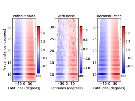
Figure 3: Left panel shows travel times corresponding to the single-cell profile (see panels a and c of Figure 4). Mid panel: travel-times of left panel are randomly perturbed in proportion with observed errors, later used for inversion are shown. Right panel: travel-time obtained using the inverted profile of the stream function using Equation (6).

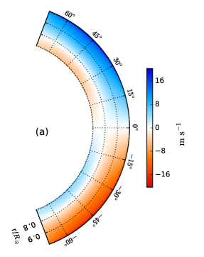
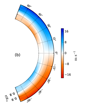
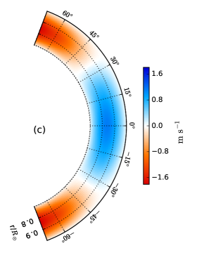
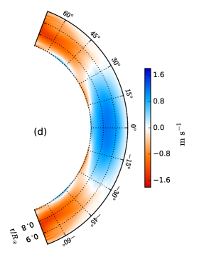
Figure 4: Synthetic inversion with a single-cell profile after including noise. We have chosen an input stream-function profile corresponding to single-cell flow. Panels a and c show profiles of $v_{\theta}$ and $v_{r}$ respectively obtained from that stream function using Equation (5) and (4). Panels b and d display the corresponding inverted profile of $v_{\theta}$ and $v_{r}$ using artificial travel times shown in Figure (3). Northward velocity is positive and vice versa.

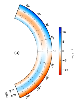
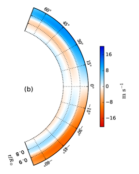
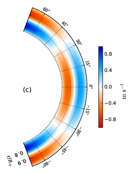
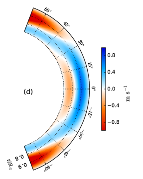
Figure 5: Synthetic inversion with a double-cell profile after including noise. Panels a and c show inputs $v_{\theta}$ and $v_{r}$ respectively whereas panels b and d display corresponding inverted profiles.

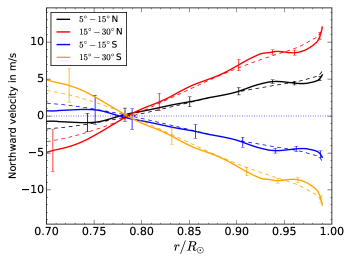
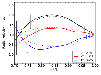
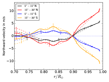
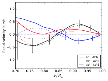
Figure 6: Synthetic inversion with noise. Depth dependence of input (dashed line) and inverted profiles (solid line) of $v_{\theta}$ (left panels) and $v_{r}$ (right panels) averaged over latitudes mentioned in plot legends are plotted with error bars. Upper panels and lower panels show results for single-cell case and double-cell case respectively.

6 Results

We use travel-time measurements of meridional circulation obtained from analyses of 6 years of observational data by SDO/HMI in the periods between 2010 to 2016. As mentioned before, we perform inversions to determine stream function $\psi$ and evaluate components of flow, $v_{r}$ and $v_{\theta}$, using Equation (4) and (5). We find similar results by using two methods as described in section (4). Inversion results are shown in Figure (7) and (8). The results are qualitatively similar to those obtained by Rajaguru & Antia (2015) using ray theory. We plot depth variations of horizontal and radial flows, $v_{\theta}$ and $v_{r}$, averaged over the latitude range described in the Figure (8). We find that the return flow is below $0.78\,R_{\odot}$ at all latitudes. Similar to Rajaguru & Antia (2015), we also see sign change in $v_{\theta}$ at low latitudes below $0.9\,R_{\odot}$. However this is not significant when considering the size of the error bar (see Figure 8). We are unable to completely rule out the picture of multiple-cell meridional circulation because of this. At higher latitudes, it clearly represents a single-cell profile. Inverted profile for radial velocity $v_{r}$ (right panel of Figure 7) suggests that flow is directed outward at lower latitude and inward at higher latitude.

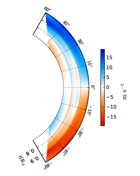
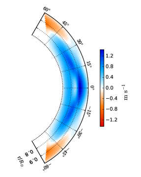
Figure 7: Meridional circulation profile after inverting observed wave travel times. Left panel shows a cross-sectional view of the horizontal component of the flow $v_{\theta}$ and the right panel shows the radial component of the flow $v_{r}$ in the $(r,\theta)$ plane.

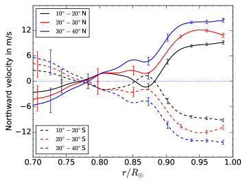
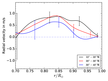
Figure 8: Meridional circulation profile. Radial dependencies of $v_{\theta}$ (left panel) and $v_{r}$ (right panel), averaged over the described latitude range with error bars.

7 Discussion and conclusion

Owing to its significant importance for the understanding of solar dynamo process, there have been several attempts using different techniques to infer meridional circulation. Due to systematic errors and associated small magnitudes, inferred models of this circulation tend to vary widely from one study to another (Zhao et al., 2013; Jackiewicz et al., 2015; Rajaguru & Antia, 2015; Böning et al., 2017; Chen & Zhao, 2017). In this work, we introduce a combination of techniques to improve the accuracy of the inference and the condition number of the inverse problem: (1) to ensure mass conservation we use stream function, (2) we compute sensitivity kernels for stream function in the first-order Born approximation and (3) we project the solution on a cubic B-spline, derivatives of Legendre-polynomial basis to reduce the number of free parameters (4) we assume hemispheric symmetry and only consider even Legendre polynomials. In order to validate this method, we test it on single and double-cell models of the meridional circulation. Surface-velocity amplitudes of these profiles are chosen so as to be close to the observational value. We compute synthetic travel times by integrating Born kernels against the stream function and add randomly generated noise in proportion to observational errors.

Upon successful validation, we apply the method to infer meridional circulation from travel-time measurements obtained from 6 years of SDO/HMI observational data. We find qualitatively similar results to those of Rajaguru & Antia (2015). Our inversion results suggest a single cell profile covering $\pm 60^{\circ}$ in latitude and up to $0.7\,R_{\odot}$ in depth in the radial direction. We find a sign change in the horizontal component of the velocity, $v_{\theta}$ beneath $0.9\,R_{\odot}$ within $\pm 20^{\circ}$ in latitude but is inconclusive considering the size of the error bar. We find equatorward return flow below $0.78\,R_{\odot}$.

Our analysis period almost exactly overlaps with analysis period of Chen & Zhao (2017). Differences in the two inversion results might be due to following factors. We have not removed surface magnetic regions in order to obtain travel time induced by solar meridional flow. Liang & Chou (2015) have demonstrated that not removing surface magnetic regions affects the travel time measurements. We have accounted for local mass conservation and also employed Born kernels, whereas Chen & Zhao (2017) have not considered mass conservation and used ray kernels.

Braun & Birch (2008) have shown that in order to infer the depth profile of a weak signal like the solar meridional flow in the entire convection zone, many years of data are needed. However, during this period, the flow might change as a function of phase of solar activity cycle. In that case, we can only obtain an average meridional flow profile for the time period of the analysis. Improvements such as including full covariance matrix as Böning et al. (2017) have suggested and accounting for line-of-sight effects (latter is only possible in wave-theoretic approach) is reserved for our future studies.

K. M acknowledges the financial support provided by the Department of Atomic Energy, India. SMH acknowledges support from Ramanujan Fellowship SB/S2/RJN-73 and the Max-Planck Partner group program.

References

- Baldner & Schou (2012) Baldner, C. S., & Schou, J. 2012, ApJ, 760, L1
- Basu & Antia (2010) Basu, S., & Antia, H. M. 2010, ApJ, 717, 488
- Basu et al. (1999) Basu, S., Antia, H. M., & Tripathy, S. C. 1999, ApJ, 512, 458
- Bhattacharya et al. (2017) Bhattacharya, J., Hanasoge, S. M., Birch, A. C., & Gizon, L. 2017, ArXiv e-prints, arXiv:1708.03464
- Birch & Felder (2004) Birch, A. C., & Felder, G. 2004, ApJ, 616, 1261
- Birch et al. (2001) Birch, A. C., Kosovichev, A. G., Price, G. H., & Schlottmann, R. B. 2001, ApJ, 561, L229
- Böning et al. (2017) Böning, V. G. A., Roth, M., Jackiewicz, J., & Kholikov, S. 2017, ApJ, 845, 2
- Böning et al. (2016) Böning, V. G. A., Roth, M., Zima, W., Birch, A. C., & Gizon, L. 2016, ApJ, 824, 49
- Braun & Birch (2008) Braun, D. C., & Birch, A. C. 2008, ApJ, 689, L161
- Chen & Zhao (2017) Chen, R., & Zhao, J. 2017, ApJ, 849, 144
- Chen & Zhao (2018) —. 2018, ApJ, 853, 161
- Choudhuri et al. (1995) Choudhuri, A. R., Schussler, M., & Dikpati, M. 1995, A&A, 303, L29
- Christensen-Dalsgaard et al. (1996) Christensen-Dalsgaard, J., et al. 1996, Science, 272, 1286
- Dikpati et al. (2010) Dikpati, M., Gilman, P. A., & Ulrich, R. K. 2010, ApJ, 722, 774
- Duvall (1979) Duvall, Jr., T. L. 1979, Sol. Phys., 63, 3
- Giles et al. (1997) Giles, P. M., Duvall, T. L., Scherrer, P. H., & Bogart, R. S. 1997, Nature, 390, 52
- Gizon et al. (2017) Gizon, L., Barucq, H., Duruflé, M., et al. 2017, A&A, 600, A35
- González Hernández et al. (2008) González Hernández, I., Kholikov, S., Hill, F., Howe, R., & Komm, R. 2008, Sol. Phys., 252, 235
- Haber et al. (2002) Haber, D. A., Hindman, B. W., Toomre, J., et al. 2002, ApJ, 570, 855
- Hathaway (2012) Hathaway, D. H. 2012, ApJ, 760, 84
- Hathaway et al. (1996) Hathaway, D. H., Gilman, P. A., Harvey, J. W., et al. 1996, Science, 272, 1306
- Jackiewicz et al. (2015) Jackiewicz, J., Serebryanskiy, A., & Kholikov, S. 2015, ApJ, 805, 133
- Komm et al. (1993) Komm, R. W., Howard, R. F., & Harvey, J. W. 1993, Sol. Phys., 147, 207
- Kosovichev & Duvall (1997) Kosovichev, A. G., & Duvall, Jr., T. L. 1997, in Astrophysics and Space Science Library, Vol. 225, SCORe’96 : Solar Convection and Oscillations and their Relationship, ed. F. P. Pijpers, J. Christensen-Dalsgaard, & C. S. Rosenthal, 241–260
- Liang & Chou (2015) Liang, Z.-C., & Chou, D.-Y. 2015, ApJ, 805, 165
- Mandal et al. (2017) Mandal, K., Bhattacharya, J., Halder, S., & Hanasoge, S. M. 2017, ApJ, 842, 89
- Pijpers & Thompson (1994) Pijpers, F. P., & Thompson, M. J. 1994, A&A, 281, 231
- Rajaguru & Antia (2015) Rajaguru, S. P., & Antia, H. M. 2015, ApJ, 813, 114
- Schad et al. (2013) Schad, A., Timmer, J., & Roth, M. 2013, ApJ, 778, L38
- Schou & Bogart (1998) Schou, J., & Bogart, R. S. 1998, ApJ, 504, L131
- Ulrich (2010) Ulrich, R. K. 2010, ApJ, 725, 658
- Woodard et al. (2013) Woodard, M., Schou, J., Birch, A. C., & Larson, T. P. 2013, Sol. Phys., 287, 129
- Zhao et al. (2013) Zhao, J., Bogart, R. S., Kosovichev, A. G., Duvall, Jr., T. L., & Hartlep, T. 2013, ApJ, 774, L29
- Zhao et al. (2012) Zhao, J., Nagashima, K., Bogart, R. S., Kosovichev, A. G., & Duvall, Jr., T. L. 2012, ApJ, 749, L5