On the Complexity Analysis of the Primal Solutions for the Accelerated Randomized Dual Coordinate Ascent
Abstract
Dual first-order methods are essential techniques for large-scale constrained convex optimization. However, when recovering the primal solutions, we need iterations to achieve an -optimal primal solution when we apply an algorithm to the non-strongly convex dual problem with iterations to achieve an -optimal dual solution, where can be or . In this paper, we prove that the iteration complexity of the primal solutions and dual solutions have the same order of magnitude for the accelerated randomized dual coordinate ascent. When the dual function further satisfies the quadratic functional growth condition, by restarting the algorithm at any period, we establish the linear iteration complexity for both the primal solutions and dual solutions even if the condition number is unknown. When applied to the regularized empirical risk minimization problem, we prove the iteration complexity of in both primal space and dual space, where is the number of samples. Our result takes out the factor compared with the methods based on smoothing/regularization or Catalyst reduction. As far as we know, this is the first time that the optimal iteration complexity in the primal space is established for the dual coordinate ascent based stochastic algorithms. We also establish the accelerated linear complexity for some problems with nonsmooth loss, i.e., the least absolute deviation and SVM.
1 Introduction
In this paper, we study the following structured constrained convex optimization problem:
| (1.1) |
where , , each and is convex and is -strongly convex. Both and can be non-differentiable. In machine learning, each column of often represents a data point. is often the loss function, e.g., for the absolute deviation and for SVM, where is the label for the -th data. is often the regularizer, e.g., the regularization and - regularization . Problem (LABEL:problem) is actually very general to incorporate many existing problems in machine learning. When dropping the constraints, problem (LABEL:problem) becomes the regularized empirical risk minimization (ERM) problem associated with linear predictors:
| (1.2) |
The ERM problem is widely used in machine learning. Please see [1, 2] for examples.
Due to the complicated constraints, people often do not solve problem (LABEL:problem) directly. Instead, they solve its dual problem by introducing the Lagrangian function. Many first-order methods can be used to solve the dual problem, e.g., the dual full gradient ascent (DFGA) [3], the accelerated DFGA (ADFGA) [4, 5], the randomized dual coordinate ascent (RDCA) [6, 7, 8, 1] and the accelerated RDCA (ARDCA) [6, 9, 10, 2]111Although the algorithm studied in this paper is a special case of APCG in [10] and APPROX in [9], we name it ARDCA to emphasize the application to the dual problem.. They need , , and iterations to achieve an -optimal dual solution, respectively, where is the dimension in the dual space. At each iteration, RDCA and ARDCA choose one coordinate to sufficiently increase the dual objective value while keeping the others fixed. The cost at each iteration of RDCA and ARDCA may be much lower than that of DFGA and ADFGA. Since both and can be non-differentiable, the dual function is non-strongly convex. So only the sublinear complexity can be obtained.
It is not satisfactory to establish the iteration complexity only in the dual space. We should recover the primal solutions from the dual iterates and need to estimate how quickly the primal solutions converge. Unfortunately, [11] established the algorithm independent result that the iteration complexity in the primal space is worse than that in the dual space. Specifically, [11] studied the following problem, which is a special case of problem (LABEL:problem),
| (1.3) |
For a pair of approximate primal-dual solution 222 is recovered form and will be defined in (LABEL:xu_solution) later., the precision between and satisfies
where is the negative of the dual function and is a pair of optimal primal-dual solution. Thus if some algorithm achieves an -optimal dual solution333We define an -optimal dual solution as . of after iterations, it only achieves an -optimal primal solution444We define an -optimal primal solution as and . can be a general norm. of after the same time. [11] studied DFGA and ADFGA and established the and iteration complexity in the primal space to find an -optimal primal solution. [12] proved the similar algorithm independent results for problem (LABEL:problem2). [13] proved the iteration complexity to achieve an -optimal primal solution for the deterministic accelerated full gradient methods for problem (LABEL:problem2).
Some researchers used regularization/smoothing to improve the iteration complexity of the primal solutions. They added a small regularization term to the dual function to smooth the primal objective and solved a regularized dual problem by some algorithm with linear convergence rate. [14] applied ADFGA to a smoothed problem of (LABEL:problem1) and [15] used ADFGA to solve a regularized dual problem of conic convex programming. However, they established the suboptimal iteration complexity of to achieve an -optimal primal solution recovered from the last dual iterate, which has an additional factor. The drawback of this strategy in practice is that it needs to choose the parameter in advance, which is related to the target accuracy. It is desirable to develop direct support for problems with non-smooth primal objective or non-strongly convex dual objective.
Other researchers improved the iteration complexities of DFGA and ADFGA in the primal space via averaging the primal solutions appropriately. [16] studied the problem of and established the iteration complexity measured by the duality gap for the accelerated full gradient method. [17] and [18] used [16]’s result for ADFGA to solve the embedded linear model predictive control problem, which is a special case of problem (LABEL:problem1). [15] proved the iteration complexity for DFGA and iteration complexity for ADFGA to achieve an -optimal averaged primal solution for conic convex programming. None of them studied the general problem (LABEL:problem) and none of them studied the methods based on randomized dual coordinate ascent.
The randomized coordinate descent and its accelerated version have received extensive attention recently for solving large-scale optimization problems since it can break down the problem into smaller pieces. [1] showed that the Stochastic Dual Coordinate Ascent (SDCA) needs iterations to reach an -optimal solution in both the primal space and dual space for problem (LABEL:problem2). [2] then developed an accelerated SDCA (ASDCA) and attained the suboptimal iteration complexity to achieve an -optimal primal solution via solving a regularized dual problem, which has the additional factor due to the smoothing/regularization technique. Catalyst [19], a general scheme for accelerating first-order optimization methods, also yields the additional factor. The Accelerated randomized Proximal Coordinate Gradient (APCG) method [10] is another famous method for problem (LABEL:problem2), which needs iterations to find a dual solution in accuracy. However, the sublinear complexity in the primal space is not established in [10]. [20] proposed a Stochastic Primal-Dual Coordinate method (SPDC) and [21] proposed a Randomized Primal-Dual Gradient method (RPDG) for problem (LABEL:problem2). They smoothed and achieved the iteration complexity. When has -Lipschitz continuous gradient, ASDCA, APCG, SPDC and RPDG all have the accelerated linear complexity of .
1.1 Contributions
In this paper, we study the iteration complexity of the primal solutions when using ARDCA to solve the non-strongly convex dual problem. Specifically, we aim to prove that the complexity of the primal solutions has the same order of magnitude as that of the dual solutions.
For the general problem (LABEL:problem), when applying ARDCA to solve its dual problem, we prove the iteration complexity of the primal solutions simply by averaging the last few primal iterates appropriately. This complexity has the same order of magnitude as that of the dual solutions and thus improves the theoretical results in [11, 12]. As a comparison, literature [16, 17, 18, 15] only studied ADFGA, which is much simpler than the analysis of ARDCA. Since we use ARDCA to solve the dual problem directly, rather than a regularized dual problem or a smoothed primal problem, our result takes out the factor compared with the smoothing/regularization based methods.
When the dual function satisfies the quadratic functional growth condition, by restarting ARDCA at any period, we prove the linear iteration complexity for both the primal solutions and dual solutions. Moreover, our analysis does not require the parameters of the algorithm depend on the condition number , which will be defined in Assumption 2 later and it is often difficult to estimate in practice. We show that ARDCA with restart outperforms RCDA for a wide range of inner iteration numbers and the optimal complexity can be attained when the inner iteration number is equal to . The difference with respect to [22] is that our analysis does not require the uniqueness of the optimal dual solution.
When applied to problem (LABEL:problem2), our work extends the theoretical results of [10] and improves those of [2]. We prove that ARDCA needs iterations to find an -optimal solution in both the primal space and dual space, while [10] only proved the iteration complexity in the dual space. This complexity matches the theoretical lower bound [23] and state-of-the-art upper bound [24]. Our theory outperforms ASDCA [2] and Catalyst [19] by the factor of . As far as we know, we are the first to establish the optimal complexity in the primal space for the dual coordinate ascent based stochastic algorithms. When has -Lipschitz continuous gradient, ARDCA with restart has the optimal complexity. Moreover, we establish the accelerated linear complexity of ARDCA with restart for some special problems with nonsmooth , e.g., the least absolute deviation problem and support vector machine (SVM).
1.2 Assumption, Notation and Problem Formulation
1.2.1 Assumption
We study problem (LABEL:problem) under the following assumptions:
Assumption 1.
1. is -strongly convex over , i.e., , for every subgradient .
2. is convex and -Lipschitz continuous over , i.e., .
3. is convex and has bounded subgradients over , i.e., , .
4. There exists such that and .
5. The optimal objective value of problem (LABEL:problem) is finite.
Assumption 1.4 is the Slater’s condition. Assumption 1.4 and 1.5 ensure that the strong duality holds, i.e., the dual optimal value is equal to the primal optimal value [25]. Assumptions 1.1 and 1.3 will be used to establish the Lipschitz smoothness of part of the dual function in Lemma 1. Assumption 1.2 will be used to get the complexity for problem (LABEL:problem) from that of the reformulated problem (LABEL:problem3).
To make each iteration of the randomized dual coordinate ascent computationally efficient, we only consider the case that is a linear function for simplicity, i.e.,
| (1.4) |
where and . However, the analysis in this paper suits for the general function satisfying Assumption 1.3.
In Section 4, we will prove the linear complexity of ARDCA with restart under the quadratic functional growth condition [26, 27]. This condition is equivalent to the error bound condition in [28, 29] and is satisfied for broad applications in machine learning, e.g., the least absolute deviation and SVM [30].
Assumption 2.
satisfies the quadratic functional growth condition with respect to the norm , i.e., , where is the condition number, is the optimal dual solution, is the projection of onto the optimal dual solution set and is the negative of the dual function.
1.2.2 Notation
Lowercase bold letters represent vectors, uppercase bold letters represent matrices and non-bold letters represent scalars. Let be the set of nonnegative vectors in and be the dimension of the dual variable. Denote and as the -th element of and , respectively. Let and be the vectors consisting of and , respectively. The value of at iteration is denoted by . For scalars, e.g., , represents its value at iteration and denotes its squares. and are the -th column and -th row of , respectively. We use as the Euclidean norm and as the infinite norm for a vector. Define the weighted norm and its dual norm . For any matrix , is the largest singular value of . () means the largest (smallest) integer less (larger) than or equal to . For a function , we use to denote its conjugate and to denote its proximal mapping. Define .
1.2.3 Problem Formulation
Reformulate problem (LABEL:problem) as
| (1.5) |
and introduce the Lagrangian function as
| (1.6) |
where is the vector of the Lagrange multipliers. Define the dual feasible set as and denote to be the optimal dual solution set. Then the Lagrange dual problem of (LABEL:problem3) can be expressed as
where
| (1.7) |
Define
| (1.11) |
where Then we can rewrite the Lagrange dual problem as
| (1.12) |
where we define and means the negative of the dual function. We study the negative of the dual function, rather than the dual function directly, since is convex. Let and be the optimal primal solution and dual solution of problem (LABEL:problem3), respectively. Then they satisfy the KKT condition [25]. Since the strong duality holds, we have . Since is strongly convex over for every , then is unique. Due to Danskin’s theorem [25] we know that is convex, differentiable and
| (1.13) |
From Proposition 3.3 in [11], we have a Lipschitz smooth condition555[11] studied the projected gradient method under the local Lipschitz smooth condition and the fast gradient method under the global Lipschitz smooth condition. The former condition is ensured by replacing Assumption 1.3 with and a further assumption that is differentiable. In this paper, we use the global Lipschitz smooth condition over the dual feasible set for simplicity. of , where
| (1.14) |
Similarly, we can also prove a coordinatewise Lipschitz smooth condition in the following lemma, whose proof is given in Appendix B.
Lemma 1.
For any and any , assume that . Then , where
| (1.15) |
2 Accelerated Randomized Dual Coordinate Ascent
In this section, we use the standard accelerated randomized coordinate descent [9, 10] to solve the dual problem (1.12), which consists of the following steps at each iteration:
At each iteration, accelerated randomized coordinate descent picks a random coordinate and generates and . Only the -th coordinate of is updated and the other coordinates remain unchanged. However, the above algorithm performs full-dimensional vector operations of and , which makes the per-iteration cost higher than the simple non-accelerated coordinate descent. To avoid such operations, we can use a change of variables scheme proposed in [32, 9]. Specifically, introduce initialized at and the new algorithms consists of the following steps at each iteration:
From Proposition 1 in [9], we know that the above two algorithms are equivalent in the sense of , and given .
Next, we discuss the computation of , and we expect that it is best times faster than the computation of . Consider the simple case of (1.4). Define
| (2.1) |
Then from the definitions in (1.11) and (LABEL:xu_solution), we have . So we can prove , and . Thus if we keep a variable and update it without the full matrix-vector multiplication, and can be efficiently computed. We describe the explicit update of in Algorithm 1. At each iteration, only the -th column of is used, rather than the full matrix . So Algorithm 1 only needs to deal with the -th constraint, rather than all the constraints at each iteration.
The only thing left to do is to compute the gradient of and the proximal mapping of . In machine learning, is often the regularizer and is the loss function. The most commonly used strongly convex regularizer is the regularization . In this case, and thus the computation time of is . We can also use some non-smooth strongly convex regularizers in the form of . In this case, , which can be efficiently computed when the proximal mapping of has closed form solution. On the other hand, when computing the proximal mapping of (or the proximal mapping of since ), we only need to solve an optimization problem with only one dimension, which can be efficiently done, e.g., by the nonsmooth Newton or quasi Newton method [33]. For many machine learning problems, the proximal mapping of can be computed efficiently (see, e.g., [1, 2]). Thus, Algorithm 1 needs about time at each iteration while DFGA and ADFGA need time.
Remark 1.
A main difference between Algorithm 1 and the original accelerated randomized coordinate descent is that Algorithm 1 uses the step-size of when computing while the original algorithm uses a larger one of , which makes the original algorithm faster than Algorithm 1 in practice. The reason of the smaller step-size is to fit the proof. Specifically, it allows us to keep an additional term in Lemma 6, which is crucial in the proof of Lemma 8. Otherwise, we may only bound for the constraint functions, rather than in Lemma 8. The former is less interesting since the expectation is inside the norm.
In Algorithm 1, we output the average of from some to 666We leave the efficient computation of the average in Appendix A., rather than . This little change allows us to give a faster convergence rate in the primal space. We average from , rather than from the first iteration, since the first few iterations often produce poor solutions. We now state our main result on the convergence rate of the primal solutions for ARDCA. Let
denote the random sequence, be the expectation with respect to and be the conditional expectation with respect to conditioned on , then we have the following theorem.
Now we compare the convergence rate of the primal solutions with that of the dual solutions. For the dual problem (1.12), [10] proved the convergence rate, which is described in the following proposition.
Thus we can see that Algorithm 1 needs iterations to achieve an -optimal primal solution and dual solution, i.e., the iteration complexity of the primal solutions has the same order of magnitude as that of the dual solutions for ARDCA.
To make a better comparison with the existing result, we describe the relation of the primal objective and constraint functions with the dual objective without averaging the primal solutions in the following proposition, which only applies to problem (LABEL:problem1). Combing with (2.2), we can immediately get the convergence rate in the primal space, which verifies that averaging the primal solutions helps to improve the convergence rate in the primal space.
3 Convergence Rate Analysis of the Primal Solutions
In this section, we prove Theorem 1. First we study a simple case in Section 3.1 to intuitively show how to relate the primal objective with the dual objective and why average helps to improve the convergence rate. Then we give the detailed analysis for the general case in Section 3.2.
3.1 Intuition: A Case Study
In this section, we study a simple case of problem (LABEL:problem):
We only consider the gradient descent to solve the dual problem for simplicity, which has the recursion of
| (3.1) |
Then and reduce to
| (3.2) |
which further leads to
| (3.3) |
(3.3) is a crucial property to relate the primal objective and dual objective. From the -smoothness of , we have
From , (3.3), (3.2) and (LABEL:GD), we have
Define , letting and summing over , we have
where we use Jensen’s inequality for in . On the other hand, from (3.2) and (LABEL:GD), we have
| (3.4) |
where we use the non-increasing of for gradient descent in . Thus, from the above two inequalities, we have
which gives the convergence rate of the primal solutions. When replacing gradient descent with accelerated gradient descent, the convergence rate can be improved to . However, more efforts are required for the analysis in the dual space and the averaging weights should be designed carefully. When solving the general problem (LABEL:problem), we should consider the separable part and the inequality constraints more carefully. When using the accelerated randomized dual coordinate ascent, we should pay more efforts to deal with the expectation, especially that the deduction in (LABEL:cont53) is not enough to deal with the constraint functions and it requires more skillful analysis. We give the detailed analysis in the following section.
From the above analysis, we can see that (3.3) is a critical trick in our analysis. To show the importance of averaging the primal solutions, we give a simple convergence rate analysis measured at the non-averaged primal solution, which is adapted from [11]. From (3.3) and , we have
So we only need to bound . From the smoothness of , we have
Thus, we have . Since for gradient descent and (3.2), we have
Generally speaking, average helps to improve the convergence rate for many algorithms. Typical examples include the Douglas-Rachford splitting and ADMM [34]. [34] proved that for the two algorithms, the and rates are tight for the non-averaged and averaged solutions, respectively.
From the above analysis for the non-averaged solutions, we can see that serves as a measure of the optimality and feasibility of the primal solutions. [35] studied how to make gradient small. Specifically, to find a point with , accelerated dual ascent needs iterations. When using some regularization technique, the complexity can be attained. We can see that none of them reaches the optimal complexity. On the other hand, when averaging the primal solutions, we do not need to make the gradient small. Instead, we only need to make the average of gradients small, i.e., in (LABEL:cont53). This is the reason why average helps to improve the convergence rate.
3.2 ARPCA for the General Problem
To better analyze the method, we give an equivalent algorithm of ARDCA and describe it in Algorithm 2. In Algorithm 2, variables are only used for analysis. In practice, we do not need to compute .
The definition of satisfies . Define , which also satisfies for . For the sequence , we can simply prove the following properties.
Lemma 2.
For the sequence satisfying and , we have
-
1.
.
-
2.
.
-
3.
.
-
4.
Letting , we have for any .
We follow [9] to define the sequence satisfying
| (3.10) |
From Lemma 2 in [9], we have , and . Define , then due to Jensen’s inequality for . We can easily verify that variables , and remain in at all times by induction, described in the following lemma. Then we can use the Lipschitz smooth condition described in Lemma 1.
Lemma 3.
For Algorithm 2, we have , and .
For Algorithm 2, let
| (3.11) |
From the optimality condition of in Algorithm 2, we have . Define
| (3.14) |
and
| (3.15) |
From the convexity of and , we have and . We use and to relate the primal objective function, primal constraint functions and dual objective function in the following lemma.
Lemma 4.
Proof.
From (1.13), (LABEL:xu_solution) and the definition of in (1.11), we have
Thus, by the definition of in (3.15), we have
From the definition of in (3.14) and the fact that , we can also have
where we use the definition of conjugate in and the fact that and in . So the result of (3.16) immediately follows by adding the above two equations and using (1.13). ∎
3.2.1 Primal Objective
In the following lemma, we use the relation (3.16) to bound the Lagrangian function . We also bound and , which will be used to bound the constraint functions later. As a by-product, we also give the convergence rate of the dual solutions.
Lemma 5.
Suppose Assumption 1 holds. Define and . Then we have
| (3.17) |
for any independent on . We also have
| (3.18) | |||
| (3.19) | |||
| (3.20) |
The proof of Lemma 5 is based on the following lemma, which gives the progress in one iteration in the dual space. Lemma 6 can be proved by the techniques in the proof of Theorem 3 in [9], except that we keep the additional terms and . We leave the proof of Lemma 6 in Appendix D.
Lemma 6.
Proof.
Dividing both sides of (LABEL:cont4) by and using , we have
| (3.22) |
Letting , we know is decreasing since and . Thus, we have
| (3.23) |
where we use and . Summing (LABEL:cont29) over and using , we have
Letting , from (3.23), and , we can immediately have (3.18), (3.19) and (3.20). On the other hand, we also have
| (3.24) |
From (3.16), for any we have
where we use the definition of and , and Jensen’s inequality for , and in . Thus, from (LABEL:cont2) and the second property in Lemma 2, we have
where we eliminate from both sides. Adding to both sides and using , we have
where we use and (3.23) in . ∎
Now we are ready to prove the convergence rate of the primal solution. We first consider the primal objective function of problem (LABEL:problem3) in the following lemma.
Lemma 7.
Proof.
Define Since , then . We also have and . Moreover, is independent on since we use in the definition, rather than . So we can let in (LABEL:cont14). Define , then we have
| (3.25) |
where we use if in , in and in . Thus, letting in (LABEL:cont14), we have
On the other hand, since is a KKT point, we have
From the definition in (1.6), we have
where we use in . So we have
| (3.26) |
which completes the proof. ∎
3.2.2 Constraint Functions
Lemma 8 establishes the convergence rate for the constraint functions of problem (LABEL:problem3). A straightforward extension of (LABEL:cont53) only leads to , which is less interesting since the expectation is inside the norm. We should take the expectation outside the norm, i.e., . The later one cannot be attained by the simple techniques in (LABEL:cont53) and requires more skillful tricks. The proof sketch of Lemma 8 is that we first establish a recursion (3.31) and then using (3.18) and the definition of in (3.30) to bound the constraint functions.
Lemma 8.
Suppose Assumption 1 holds. Define and . Then we have
| (3.27) |
Proof.
From the update of and the definitions of and in (3.11) and (1.13), we have
| (3.28) | |||
Define such that then we have
| (3.29) |
and
Define and such that
| (3.30) |
then we get and . Moreover, for , we have
where we use (3.29) and (3.30) in and (7.2) in . Then for any , we have
| (3.31) |
Summing over and using , we have
| (3.32) |
where we use (3.18) in . On the other hand, from the definition of and , we have
So from (3.32), (3.19) and (3.23), we have
| (3.33) |
For , we have
| (3.34) |
Similarly, for , we have
and for , we have
Then we have
Taking expectation with respect to and from (LABEL:cont32), we can immediately have the conclusion. ∎
3.2.3 Proof of Theorem 1
| (3.35) |
we have
From Cauchy-Schwartz inequality, we have the desired result.
Remark 2.
4 Extension under the Quadratic Growth Condition
In this section, we give the linear complexity under stronger assumptions. Specifically, we use both Assumptions 1 and 2 in this section. The quadratic functional growth condition in Assumption 2 is equivalent to the global error bound condition [29] and is satisfied for broad applications. We give a simple example satisfying Assumption 2 and refer the reader to [36, 37, 38, 39] for more examples.
Example. Consider problem (LABEL:problem) with strongly convex and smooth and the simple form (1.4) of . Furthermore, we require that has the form of , where is a polyhedral function or an indicator function of a polyhedral set. In this case, , where and are defined in (2.1). It may not be strongly convex since may not be full column rank. However, satisfies the error bound condition [28, 30] and thus satisfies Assumption 2. The least absolute deviation, SVM and multiclass SVM [2] have the required form.
To exploit Assumption 2, we use Algorithm 1 with restart [40, 22] and establish the faster convergence rate. Namely, at each iteration, Algorithm 1 is called with fixed and finite iterations with the output of the previous iteration being the initializer of current iteration. We describe the method in Algorithm 3. We use the inner-outer iteration procedure, rather than the one loop accelerated algorithms with direct support to strongly convex dual functions, e.g., APCG [10], since the quadratic functional growth condition is generally not enough to prove the accelerated linear convergence rate for the one loop accelerated algorithms [26].
Define to be the nearest optimal solution to . Denote and to be the random sequence, where is the random index chosen at the -th outer iteration and -th inner iteration of Algorithm 3. We give the linear convergence of Algorithm 3 for both primal solutions and dual solutions in Theorem 2.
Theorem 2.
In the traditional analysis for the restart scheme, the inner iteration number heavily depends on the condition number [41, 22]. Specifically, letting in (3.20) and from Assumption 2, we have
To make , we should require , otherwise, the traditional analysis cannot prove the decrement of the objective. However, in practice, is often difficult to estimate. Different from the traditional analysis, in Theorem 2, we show the linear convergence when the algorithm restarts at any period. In other words, for any . Our analysis applies to the problems where is unknown.
Remark 3.
Our result (4.1) is motivated by [22]. However, when applied to the dual problem (1.12), [22] requires that has the unique optimal dual solution and needs a stronger quadratic functional growth condition of
| (4.3) |
As a comparison, in Assumption 2, we do not need the uniqueness of the optimal dual solution and only assume
| (4.4) |
Comparing (4.4) with (4.3), we can see that (4.3) can deduce (4.4) and not vice versa. The analysis in [22] cannot be applied under our assumptions since a critical property in [22, Equ. (28)] does not hold any more. To deal with the more general assumption (4.4), we develop a totally different proof framework and it is much simpler and more general.
Let us compare the complexity of Algorithm 3 with that of randomized dual coordinate ascent, i.e., [7]. If , Algorithm 3 attains the optimal complexity of for both the primal solutions and dual solutions when . When , Algorithm 3 outperforms the randomized dual coordinate ascent777Please see the details in Appendix F.. When is larger than , Algorithm 3 performs worse than randomized dual coordinate ascent. On the other hand, if , the complexity of Algorithm 3 has the same order of magnitude as that of randomized dual coordinate ascent when . When , Algorithm 3 performs worse. For most practical problems, we have and thus Algorithm 3 is a better and safe choice for a wide range of .
4.1 Convergence Rate Analysis of the Dual Solutions
In this section, we prove (4.1). We first consider one outer iteration of Algorithm 3 and use the symbols in Algorithm 2 for simplicity. In the following lemma, we show that is the convex combination of and .
Lemma 9.
Proof.
For Algorithm 2, we have
| (4.7) |
Decomposing term into and and using (4.7) for the later one, we have
Decomposing into and and using (4.7) for the later one again, we have
Do the above operations recursively, we have
where we use and in . On the other hand, we can easily check that
which leads to (4.6). Next, we prove , which is equivalent to , which is true since . ∎
Based on Lemma 9, we can establish the decreasing of for any in the following lemma. The proof sketch of Lemma 10 is that we first establish a recursion (LABEL:cont44) based on Lemma 9 and (3.20) and then prove the result in Lemma 10 by induction.
Proof.
We consider . Decomposing the second term into and and using Assumption 2 for the first term, we have
| (4.8) |
From the definition of , (4.6) and (4.5), we have
Plugging it into (LABEL:cont42) and letting , we have
| (4.9) |
where we denote for simplicity and use (3.20) with in . On the other hand, decomposing into and , using Assumption 2 for the first term and letting , we have
Plugging it into (LABEL:cont43), we have
| (4.10) |
Next, we prove by induction. From (LABEL:cont44), we have . Assume that holds for . Now, we consider . From (LABEL:cont44), we have
| (4.11) |
We can easily check
and
where we use in . Plugging them into (4.11), we only need to prove
| (4.12) |
After some simple calculations, (4.12) is equivalent to
Since , we only need to ensure and . Both inequalities hold for any and any . ∎
4.2 Convergence Rate Analysis of the Primal Solutions
In this section, we prove (LABEL:cont54). We first establish the relation between the primal objective and dual objective in the following lemma and then (LABEL:cont54) can be attained by Lemmas 10 and 11 immediately.
Lemma 11.
Proof.
We denote to be the variables at the -th outer iteration of Algorithm 3, which are the counterparts of and in Algorithm 1. Choose and let in (LABEL:cont14), which is independent on conditioned on . For the -th outer iteration of Algorithm 3, we have
Taking expectation with respect to and using the forth property of Lemma 2, we have
| (4.13) |
Choosing in (3.27) and using a similar induction, we have
| (4.14) |
Now, we consider the objective function. From (4.13) and the definition in (1.6), we have
Since satisfies the KKT condition, we have . is convex with respect to and -strongly convex with respect to , so we have
which leads to and
| (4.15) |
Let be the index set such that for any , we have and . So we have
where in we use from the complementary slackness in the KKT condition. From Assumption 1.3 and (1.15), we have , which leads to . In , we use , (4.14) and (4.15). From (4.13), we have
From , (LABEL:cont7), (4.14), (LABEL:cont48) and , we have the conclusion. ∎
5 Application to the Regularized ERM
The regularized empirical risk minimization problem (LABEL:problem2) has broad applications in machine learning. For the special problem (LABEL:problem2), its dual problem (1.12) becomes
| (5.1) |
We follow [1, 2] to assume , which can be guaranteed by normalizing the data. Then we have and from (1.14) and (1.15). From Lemmas 21 and 22 in [1], we have , and , which leads to and . We will discuss the iteration complexity of ARDCA in three scenarios.
5.1 Strongly Convex and Nonsmooth , Convex and Nonsmooth
From Theorem 1, we know that the convergence rate of ARDCA for problem (LABEL:problem2) is:
In order to have the convergence rate for ARDCA, we should find an initializer good enough such that . We use ARDCA with fixed , i.e., non-accelerated RDCA, to find such initializer. Specifically, we describe the method in Algorithm 4. Lemma 12 establishes the convergence rates of both the primal solutions and dual solutions for the first step of Algorithm 4, whose proof is given in Appendix E.
Lemma 12.
An immediate consequence of Lemma 12 is that if , we only need to run step 1 of Algorithm 4 with linear complexity to achieve an -optimal solution. We describe the results in Corollary 3. However, in statistical learning, is usually on the order of or [42, 20], thus is often not too small. In the following discussions, we only consider the case of .
Corollary 3.
If , we only need to run ARDCA(,0,) with fixed , i.e., non-accelerated RDCA, for iterations to find an -optimal solution such that
If , Algorithm 4 needs iterations to find an -optimal solution such that
Algorithm 1 is a special case of APCG [10]. [10] only established the iteration complexity in the dual space to achieve an -optimal dual solution888When has Lipchitz continuous gradient, [10] proved the linear convergence rate in the primal space. However, when is only Lipchitz continuous, the convergence rate in the primal space is not established in [10]., where . [2] developed an accelerated SDCA with an inner-outer iteration procedure, where the outer loop is a full-dimensional accelerated proximal point method. At each iteration of the outer loop, SDCA is called to solve a subproblem inexactly. ASDCA is mainly used for the problems with smooth . When is nonsmooth, [2] used ASDCA to solve a smoothed problem of (LABEL:problem2), i.e., a regularized problem of (5.1), and achieved a slightly worse iteration complexity of to find an -optimal primal solution. We can also use Catalyst [19] to solve the problems with nonsmooth without using smoothing. However, Catalyst also yields the additional factor. To make ASDCA faster than SDCA, which has the complexity [1], [2] required . Katyusha [24], a primal-only algorithm, obtains the state-of-the-art iteration complexity of , which is worse than our result when . Our result matches the theoretical lower bound of [23] when ignoring the constant term of . All the compared methods need runtime at each iteration.
5.2 Strongly Convex and Nonsmooth , Convex and Smooth
When each is -smooth, which is defined as , then is -strongly convex and is -strongly convex. In this case, Assumption 2 is satisfied with . From the discussion at the end of Section 4, we know that Algorithm 3 needs iterations in total to achieve an -optimal primal solution and dual solution in the best case scenario, which matches or outperforms the complexities of the dual based stochastic algorithms established in [10, 2]. Specifically, their complexities are and , respectively. To make the accelerated algorithms faster than the non-accelerated counterparts, [2] required (i.e., ). Thus, our complexity has a better dependence on than [2]. Note that APCG [10] needs an extra proximal full gradient step to establish the linear convergence rate in the primal space. Our analysis does not need such an additional operation. On the other hand, [10] and [2] did not study the case when is unknown.
5.3 Strongly Convex and Smooth , Convex and Nonsmooth
As discussed in Section 4, Assumption 2 is weaker than the strong convexity of and some special cases of problem (LABEL:problem) with nonsmooth also satisfy Assumption 2. We take SVM and the least absolute deviation as examples. The primal problem and dual problem of SVM are
| (5.4) |
where and is the label for the -th data , [30] proved that in (LABEL:svm_problem) satisfies the global error bound condition. From [29], we know that Assumption 2 holds. From the discussion at the end of Section 4, we can see that Algorithm 3 needs iterations in total to achieve an -optimal primal solution and dual solution in the best case scenario. As a comparison, [27] studied the randomized coordinate descent and established the iteration complexity. The better dependence on in our iteration complexity is significant when is small and this is often the case in practice. We refer the reader to Section 5 of [27] for the discussion on the size of . When is unknown, Algorithm 3 is still a better choice for a wide range of inner iteration number than the randomized coordinate descent.
For the least absolute deviation, its primal problem and dual problem are
| (5.5) |
6 Numerical Experiments
In this section, we test the performance of Algorithms 1, 3 and 4 on the sparse recovery problem. Consider the sparse linear regression problem of , where is the unknown sparse vector to estimate, is the observation and is some additive noise. A particular instance of this problem is compressed sensing [43]. In order to recovery , a popular regularization is the -norm, in which case people often solve the following problems:
where . We add the term to make the objective function strongly convex and thus we can use some fast convergent algorithms. When the noise is generated from the Gaussian distribution, people often use the loss function, i.e., . When the noise is sparse and the data contains some outliers, the loss is often used, i.e., . When the noise is generated from a uniform distribution, we often use the loss instead. In this section, we solve the following three problems
| (6.1) | |||
| (6.2) | |||
| (6.3) |
Problems (6.1) and (6.2) are special cases of problem (LABEL:problem2) satisfying the assumptions in Sections 5.2 and 5.1 and problem (6.3) is a special case of problem (LABEL:problem1), respectively. In our numerical experiment, we set , and . We generate the entries of from the uniform distribution in and normalize each column of such that . We set entries of to be nonzeros. is generated by , where we generate each entry of noise from the Gaussian distribution for problem (6.1), generate entries of from and set the others to be 0 for problem (6.2), and generate each entry of from the uniform distribution in for problem (6.3). We vary in the range in problems (6.1) and (6.2) and in the range in problem (6.3).
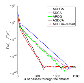
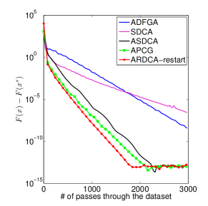
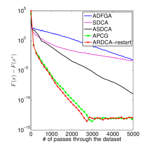
For problem (6.1), we compare ARDCA-restart (Algorithm 3) with ASDCA [2], APCG [10], SDCA [1] and ADFGA [4]. Figure 1 plots the primal gap as functions of the number of passes over the data, where each (inner) iterations are equivalent to a single pass over the data for APCG and SDCA (ARDCA and ASDCA). We use the maximal dual objective value produced by the compared methods to approximate the optimal primal objective value . We can see that ARDCA-restart outperforms the non-accelerated SDCA and non-randomized ADFGA for a wide range of and ARDCA-restart is superior to APCG and ASDCA for some values of .
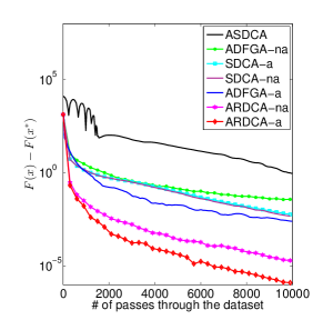
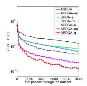
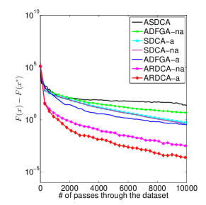
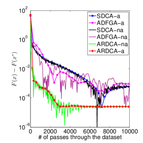
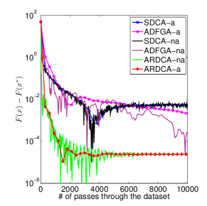
For problem (6.2), we compare ARDCA (Algorithm 4) with ASDCA [2], SDCA [1] and ADFGA [4], where ASDCA solves a regularized dual problem of (6.2) by adding term to the dual objective with . We set in Algorithm 1. Figure 2 plots the results, where ARDCA-a means that we test the averaged primal solution and ARDCA-na means the non-averaged primal solution. We can see that ARDCA-a yields the best result by orders of magnitude. Specially, ASDCA with regularization does not perform well although it converges linearly when is smooth. Thus, although the regularization/smoothing based ASDCA has the near optimal theoretical result (the sub-optimality comes from the factor), its practical performance is not satisfactory.
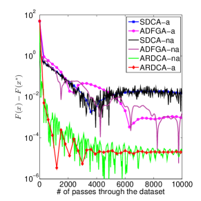
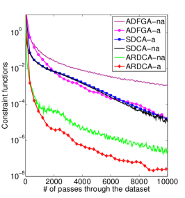
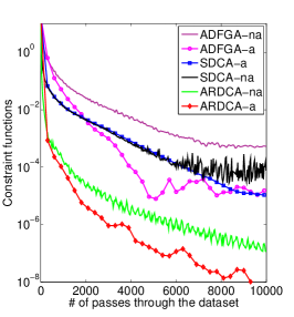
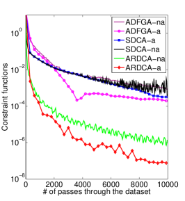
For problem (6.3), we compare ARDCA with SDCA and ADFGA. As demonstrated in Figure 4, we can see that ARDCA-a performs the best in both reducing the primal gap and constraint function value.
 |
 |
 |
 |
 |
 |
 |
 |
 |
 |
 |
 |
|
|
|
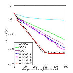
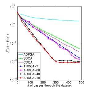
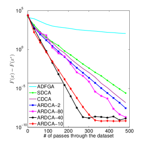
At last, we consider problem (6.2) with to verify the conclusions in Section 5.3. In this scenario, we generate to be a dense vector. We compare ARDCA with restart (Algorithm 3) with SDCA [1], the Cyclic Dual Coordinate Ascent (CDCA) [30] and ADFGA [4]. Since the quadratic functional growth parameter is unknown, we test Algorithm 3 with different inner iteration number . From Figure 3 we can see that ARDCA, SDCA and CDCA all converge linearly and ARDCA with suitable performs the best. This verifies our theories in Section 5.3.
7 Conclusion
In this paper, we prove that the iteration complexities of the primal solutions and dual solutions have the same order of magnitude for the accelerated randomized dual coordinate ascent. Specifically, when is -strongly convex and the objectives are nonsmooth, we establish the iteration complexity. When the dual function further satisfies the quadratic functional growth condition, we prove the linear iteration complexity even if the condition number is unknown. When applied to the regularized empirical risk minimization problem, we prove the iteration complexity of , which outperforms the existing results by a factor. We also prove the accelerated linear convergence rate for some special problems with nonsmooth loss, e.g., the least absolute deviation and SVM. All the above results are established for both the primal solutions and dual solutions. The topic on the complexity analysis of the primal solutions is significant not only in stochastic optimization but also in distributed optimization. We hope that the analysis in this paper could facilitate more studies on this topic.
Appendix A: Efficient Computation of the Average
We discuss the efficient computation of . We define two variables and , update and at each iteration of Algorithm 1. We only store and when . When the algorithm terminate at the -th iteration, we let such that and compute . Thus, we only need computation time at each iteration and storage space in total, where is the dimension of .
Appendix B: Proof of Lemma 1
Proof.
Let . From the proof of Theorem 3.1 in [11], we have
If , then we have
If , then we have
which completes the proof. ∎
Appendix C: Proof of Lemma 2
Proof.
From , we can immediately prove the first two properties. We also have , which leads to . So we get by letting for any . ∎
Appendix D: Proof of Lemma 6
Lemma 6 can be proved by the techniques in [9] with only a little changes. We give the proof for the sake of completeness.
Proof.
From the optimality condition of , we have
Thus, for any and any , we have
| (7.1) |
where we use the convexity of for and the definition of for . Since , and , then from (1.16), we have
Using the relations of and in Algorithm 2, we have
Taking expectation with respect to conditioned on , we have
where we use the convexity of in , the definition of in , (7.1) in , in and the following three equations in , which can be obtained from Lemma 4 and Equation (45) in [9],
| (7.2) |
Rearranging the terms, we have
Taking expectation with respect to on both sides, we have
Since , , are independent on and , , , , , are independent on , we have (LABEL:cont4). ∎
Appendix E: Proof of Lemma 12
.
Appendix F: Analysis for the Complexity Comparisons in Section 4
Letting be a constant, e.g., 2, we have and . So and (7.4) has the same order of magnitude as .
When , (7.4) has the same order of magnitude as and it is smaller that .
When , (7.4) has the same order of magnitude as and it is also smaller than .
Case 2: .
(7.4) has the same order of magnitude as when .
References
- [1] Shai Shalev-Shwartz and Tong Zhang. Stochastic dual coordinate ascent methods for regularized loss minimization. Journal of Machine Learning Research, 14(1):567–599, 2013.
- [2] Shai Shalev-Shwartz and Tong Zhang. Accelerated proximal stochastic dual coordinate ascent for regularized loss minimization. Mathematical Programming, 155(1):105–145, 2016.
- [3] Paul Tseng. Dual ascent methods for problems with strictly convex costs and linear constraints: A unified approach. SIAM J. on Optimization, 28(1):214–242, 1990.
- [4] Amir Beck and Marc Teboulle. Fast dual proximal gradient algorithm for convex minimization and applications. Operations Research Letters, 42:1–6, 2014.
- [5] Bohuang Huang, Shiqian Ma, and Donald Goldfarb. Accelerated linearized Bregman method. Journal of Scientific Computing, 54(2-3):428–453, 2013.
- [6] Yurii Nesterov. Efficiency of coordinate descent methods on huge-scale optimization problems. SIAM J. on Optimization, 22(2):341–362, 2012.
- [7] Zhaosong Lu and Lin Xiao. On the complexity analysis of randomized block-coordinate descent methods. Mathematical Programming, 152:615–642, 2015.
- [8] Peter Richtárik and Martin Takáč. Iteration complexity of randomized block-coordinate descent methods for minimizing a composite function. Mathematical Programming, 144(1-2):1–38, 2014.
- [9] Olivier Fercoq and Peter Richtárik. Accelerated, parallel, and proximal coordinate descent. SIAM J. on Optimization, 25:1997–2023, 2015.
- [10] Qihang Lin, Zhaosong Lu, and Lin Xiao. An accelerated randomized proximal coordinate gradient method and its application to regularized empirical risk minimization. SIAM J. on Optimization, 25(4):2244–2273, 2015.
- [11] Jie Lu and Mikael Johansson. Convergence analysis of aproximate primal solutions in dual first order methods. SIAM J. on Optimization, 26(4):2430–2467, 2016.
- [12] Celestine Dünner, Simone Forte, Martin Takác, and Martin Jaggi. Primal-dual rates and certificates. In ICML, 2016.
- [13] Donghwan Kim and Jeffrey A. Fessler. Fast dual proximal gradient algorithms with rate for convex minimization. In arxiv:1609.09441, 2016.
- [14] Olivier Devolder, Francois Glineur, and Yurii Nesterov. Double smoothing technique for large-scale linearly constrained convex optimization. SIAM J. on Optimization, 22:702–727, 2012.
- [15] Ion Necoara and Andrei Patrascu. Iteration complexity analysis of dual first-order methods for conic convex programming. Optimization Methods and Software, 31:645–678, 2016.
- [16] Paul Tseng. On accelerated proximal gradient methods for convex-concave optimization. Technical report, University of Washington, Seattle, 2008.
- [17] Ion Necoara and Valentin Nedelcu. Rate analysis of inexact dual first-order methods application to dual decomposition. IEEE Trans. on Automatic Control, 59:1232–1243, 2014.
- [18] Panagiotis Patrinos and Alberto Bemporad. An accelerated dual gradient projection algorithm for embedded linear model predictive control. IEEE Trans. on Automatic Control, 59:18–33, 2013.
- [19] Hongzhou Lin, Julien Mairal, and Zaid Harchaoui. A universal Catalyst for first-order optimization. In NIPS, 2015.
- [20] Yuchen Zhang and Lin Xiao. Stochastic primal-dual coordinate method for regularized empirical risk minimization. Journal of Machine Learning Research, 18(1):2939–2980, 2017.
- [21] Guanghui Lan and Yi Zhou. An optimal randomized incremental gradient method. Mathematical Programming, 2017.
- [22] Olivier Fercoq and Zheng Qu. Restarting the accelerated coordinate descent method with a rough strong convexity estimate. In arxiv:1803.05771, 2018.
- [23] Blake Woodworth and Nathan Srebro. Tight complexity bounds for optimizing composite objectives. In NIPS, 2016.
- [24] Zeyuan Allen-Zhu. Katyusha: The first direct acceleration of stochastic gradient methods. In STOC, 2017.
- [25] Dimitri Bertsekas. Nonlinear Programming. Athena Scientific, Belmont, Ma, 1999.
- [26] I. Necoara, Yu. Nesterov, and F. Glineur. Linear convergence of first order methods for non-strongly convex optimization. Mathematical Programming, 175(1-2):69–107, 2019.
- [27] Chenxin Ma, Rachael Tappenden, and Martin Takác̆. Linear convergence of randomized feasible descent methods under the weak strong convexity assumption. Journal of Machine Learning Research, 230(17):1–24, 2016.
- [28] Zhiquan Luo and Paul Tseng. On the linear convergence of descent methods for convex essentially smooth minimization. SIAM J. on Control and Optimization, 30(2):408–425, 1992.
- [29] Dmitriy Drusvyatskiy and Adrian S. Lewis. Error bounds, quadratic growth, and linear convergence of proximal methods. Mathematics of Operations Research, 2018.
- [30] Powei Wang and Chih-Jen Lin. Iteration complexity of feasible descent methods for convex optimization. Journal of Machine Learning Research, 15:1523–1548, 2014.
- [31] Yurii Nesterov. Introductory Lectures on Convex Optimization. Springer Science Business Media, 2004.
- [32] Yin Tat Lee and Aaron Sidford. Efficient accelerated coordinate descent methods and faster algorithms for solving linear systems. In FOCS, 2013.
- [33] Adrian S. Lewis and Michael L. Overton. Nonsmooth optimization via quasi-newton methods. Mathematical Programming, 141(1-2):135–163, 2013.
- [34] Damek Davis and Wotao Yin. Convergence rate analysis of several splitting schemes. Splitting Methods in Communication, Imaging, Science, and Engineering, pages 115–163, 2017.
- [35] Yurii Nesterov. How to make the gradients small. Optima, 88, 2012.
- [36] Jérôme Bolte, Trong Phong Nguyen, Juan Peypouquet, and Bruce W. Suter. From error bounds to the complexity of first-order descent methods for convex functions. Mathematical Programming, 165(2):471–507, 2017.
- [37] Guoyin Li. Global error bounds for piecewise convex polynomials. Mathematical Programming, 137(1-2):37–64, 2013.
- [38] Weihong Yang. Error bounds for convex polynomials. SIAM J. on Optimization, 19(4):1633–1647, 2009.
- [39] Mingrui Liu and Tianbao Yang. Adaptive accelerated gradient converging method under hölderian error bound condition. In NIPS, 2017.
- [40] B. O’Donoghue and E. Candès. Adaptive restart for accelerated gradient schemes. Foundations of Computational Mathematics, 15(3):715–732, 2015.
- [41] Olivier Fercoq and Zheng Qu. Adaptive restart of accelerated gradient methods under local quadratic growth condition. In arxiv:1709.02300, 2017.
- [42] Olivier Bousquet and André Elisseeff. Stability and generalization. Journal of Machine Learning Research, (2):499–526, 2002.
- [43] Emmanuel Candes, Justin Romberg, and Terence Tau. Stable signal recovery from incomplete and inaccurate measurements. Communications on Pure and Applied Mathematics, 59(8):1207–1223, 2006.