Provably Positive Discontinuous Galerkin Methods for Multidimensional Ideal Magnetohydrodynamics

Abstract

The density and pressure are positive physical quantities in magnetohydrodynamics (MHD). Design of provably positivity-preserving (PP) numerical schemes for ideal compressible MHD is highly desirable, but remains a challenge especially in the multidimensional cases. In this paper, we first develop uniformly high-order discontinuous Galerkin (DG) schemes which provably preserve the positivity of density and pressure for multidimensional ideal MHD. The schemes are constructed by using the locally divergence-free DG schemes for the symmetrizable ideal MHD equations as the base schemes, a PP limiter to enforce the positivity of the DG solutions, and the strong stability preserving methods for time discretization. The significant innovation is that we discover and rigorously prove the PP property of the proposed DG schemes by using a novel equivalent form of the admissible state set and very technical estimates. Several two-dimensional numerical examples further confirm the PP property, and demonstrate the accuracy, effectiveness and robustness of the proposed PP methods.

35L65, 65M60, 65M08, 76W05

1 Introduction

In this paper, we would like to develop the high-order numerical methods which provably preserve the positivity of density, pressure and internal energy for the ideal magnetohydrodynamics (MHD). In the laboratory frame, the equations governing the $d$-dimensional ideal compressible MHD flows can be written as a set of nonlinear hyperbolic conservation laws

(1) $$\frac{{\partial{\bf U}}}{{\partial t}}+\sum\limits_{i=1}^{d}{\frac{{\partial{{\bf F}_{i}}({\bf U})}}{{\partial x_{i}}}}={\bf 0},$$

where $d=1,2$ or $3$. In Eq. (1), the conservative vector ${\bf U}=(\rho,\rho{\bf v},{\bf B},E)^{\top}$, and ${\bf F}_{i}({\bf U})$ is the flux in the $x_{i}$-direction, $i=1,\cdots,d$, defined by

$${\bf F}_{i}({\bf U})=\Big{(}\rho v_{i},~{}\rho v_{i}{\bf v}-B_{i}{\bf B}+p_{tot}{\bf e}_{i},~{}v_{i}{\bf B}-B_{i}{\bf v},~{}v_{i}(E+p_{tot})-B_{i}({\bf v}\cdot{\bf B})\Big{)}^{\top}.$$

Here $\rho$ denotes the density, ${\bf v}=(v_{1},v_{2},v_{3})$ is the fluid velocity, ${\bf B}=(B_{1},B_{2},B_{3})$ is the magnetic field, $p_{\rm tot}$ denotes the total pressure consisting of the gas pressure $p$ and magnetic pressure $p_{m}=\frac{|{\bf B}|^{2}}{2}$, the vector ${\bf e}_{i}$ is the $i$-th row of the unit matrix of size 3, $E=\rho e+\frac{1}{2}\left(\rho|{\bf v}|^{2}+|{\bf B}|^{2}\right)$ denotes the total energy consisting of kinetic, thermal and magnetic energies, and $e$ is the specific internal energy. An additional equation for the thermodynamical quantities—the so-called equation of state (EOS)—is required to close the system (1). For ideal gases the EOS is given by

(2) $$p=(\gamma-1)\rho e,$$

where $\gamma>1$ is the adiabatic index. Although the EOS (2) is widely used, there are scenarios where it is more suitable to use other EOSs. A general EOS may be expressed as

(3) $$p=p(\rho,e).$$

We assume (3) satisfy

(4) $$\mbox{if}\quad\rho\geq 0,\quad\mbox{then}\quad e>0~{}\Leftrightarrow~{}p(\rho,e)>0.$$

Such a condition is reasonable and holds for the ideal EOS (2). It was also used in [57] to develop positive high-order schemes for the Euler equations with a general EOS.

The exact solution of the $d$-dimensional MHD equations (1) must also satisfy the following divergence-free condition on the magnetic field

(5) $$\nabla\cdot{\bf B}:=\sum\limits_{i=1}^{d}\frac{\partial B_{i}}{\partial x_{i}}=0,$$

if the initial magnetic field is divergence-free. Most of numerical methods for the multidimensional MHD equations, however, lead to a nonzero divergence of numerical magnetic field due to truncation errors, even if the initial condition satisfies (5). Existing evidences indicate that negligence in dealing with the divergence-free condition (5) can cause nonphysical features or numerical instabilities in computed solutions; see, for example, [10, 21, 5, 40, 19, 28]. Up to now, a number of numerical techniques have been developed to enforce the divergence-free condition or reduce the divergence-error in discrete sense. They include but are not limited to: the hyperbolic divergence cleaning methods [19], the projection method [10], the locally divergence-free methods (cf. [28, 52]), the constrained transport method [21] and its variants (e.g., [38, 5, 33, 2, 39, 37, 30, 29, 16]), and the eight-wave methods (e.g., [34, 35, 12, 32]). The eight-wave method was first proposed by Powell [34, 35], based on a proper discretization of the Godunov form [23] of ideal MHD equations

(6) $$\frac{{\partial{\bf U}}}{{\partial t}}+\sum\limits_{i=1}^{d}{\frac{{\partial{{\bf F}_{i}}({\bf U})}}{{\partial x_{i}}}}=-\big{(}\nabla\cdot{\bf B}\big{)}~{}{\bf S}({\bf U}),$$

where ${\bf S}=\big{(}0,~{}{\bf B},~{}{\bf v},~{}{\bf v}\cdot{\bf B}\big{)}^{\top}.$ In the literature, (6) is sometimes also called Powell’s system. The right-hand side term of (6), abbreviated as “GP source term” in the following, is proportional to $\nabla\cdot{\bf B}$ and thus identically zero if $\nabla\cdot{\bf B}=0$. This means (6) and (1) are equivalent under the condition (5). However, for the following reasons it is sometimes advantageous to add the GP source term in the equations. First, Godunov [23] pointed out that (6) is the unique form of MHD equations which is symmetrizable. The symmetrized form is useful for designing entropy stable schemes [6, 7, 12, 32]. Powell [34] noticed that the system (1) is incompletely hyperbolic and should add the source term to recover the missing eigenvector. Besides, when $\nabla\cdot{\bf B}\neq 0$, the system (1) is not Galilean invariant, while the GP source term renders the system (6) Galiean invariant (cf. [20]). In most of numerical schemes the condition (5) is only satisfied up to a discretization error. As demonstrated by Powell [35], the inclusion of GP source term assures that those small divergence-errors are consistently accounted in a numerically stable way and do not lead to accumulation of inaccuracies. This makes the eight-wave method stable to control the divergence-error, although some drawbacks [40] may be caused due to the loss of conservativeness.

Besides controlling the divergence-error, another numerical challenge for MHD is to preserve the positivity of density and pressure. In physics, these two quantities are always nonnegative. Numerically their positivity is very important, but not always satisfied by the numerical solutions. In fact, as soon as negative density or pressure is obtained in the MHD simulations, the discrete problem becomes ill-posed, causing the breakdown of codes. However, most existing MHD methods are generally not positivity-preserving (PP), and thus may suffer from a large risk of failure in solving MHD problems with low density, low pressure, low plasma-beta or strong discontinuity. A few efforts were made to reduce this risk. By switching the Riemann solvers for different wave situations, Balsara and Spicer [4] proposed a strategy to maintain the positive pressure. In [26], Janhunen noticed the difficulty of developing PP schemes based on the conservative MHD system (1), so he proposed a modified MHD system, which is similar to the Godunov form (6) but includes only the source term in the induction equation. Based on this modified system, Janhunen [26] designed an approximate 1D Riemann solver, and numerically demonstrated its PP property. Bouchut et al. [8] derived several approximate Riemann solvers for 1D ideal MHD, with sufficient conditions for those solvers to satisfy the discrete entropy inequalities and PP property. Those sufficient conditions are satisfied by explicit wave speed estimates in [9], where the Riemann solvers were implemented and multidimensional extension was discussed with the aid of Janhunen’s modified system. Waagan [41] developed a positive second-order scheme for the ideal MHD based on the approximate Riemann solver of [8, 9] and a new linear reconstruction. The robustness of that scheme was further demonstrated in [42] by extensive benchmark tests and comparisons. Recent years have witnessed significant progresses in developing high-order bound-preserving methods for hyperbolic systems (see, e.g., [54, 55, 48, 56, 25, 50, 31, 51, 44, 53]) including the ideal MHD system [3, 13, 15, 14] and the relativistic MHD system [46]. Two PP limiting techniques were developed in [3, 13] for the finite volume or discontinuous Galerkin (DG) methods for (1) to enforce the admissibility of the reconstructed or DG solutions at certain nodal points. Those techniques are built on a presumed proposition that the cell-averaged solutions of those schemes are always admissible. Such a proposition has not been rigorously proved for those schemes [3, 13], although it could be deduced for the 1D schemes in [13] under some assumptions (see a discussion in [43, Remark 2.12]). In fact, unfortunately, a usual way of using PP limiter does not necessarily ensure the PP property of the standard conservative DG schemes for multidimensional MHD system (1); see [43] for a rigorous analysis. Based on the presumed PP property of the Lax–Friedrichs (LF) scheme, Christlieb et al. [15, 14] developed PP high-order finite difference weighted essentially non-oscillatory schemes for (1) by extending the flux limiters in [50, 49].

It was numerically demonstrated that all the above PP techniques could improve the robustness of the MHD codes. However, there were few theoretical evidences, especially in the multidimensional cases, to genuinely and completely prove the PP property of those or any other schemes for (1). Very recently, rigorous PP analysis was first carried out in [43] for conservative finite volume and DG schemes with the LF flux. The analysis showed in theory that the divergence-free condition (5) is strongly connected with the PP property of numerical schemes for (1), and found that a discrete divergence-free (DDF) condition is necessary and crucial for designing the PP conservative schemes for (1). It was also proved in [43] that even the first-order multidimensional LF scheme for (1) is not PP, if the proposed DDF condition is slightly violated. Moreover, the DDF condition cannot be ensured by using a locally divergence-free basis [28]. (Note that the first-order LF scheme is locally divergence-free.) This implies, in the multidimensional cases, a usual PP limiter (e.g., [13]) does not guarantee the PP property of the standard DG schemes for the conservative MHD system (1), even if the locally divergence-free DG element [28] is used.

Interestingly, on the other hand, in the PDE level the preservation of positivity and the divergence-free condition (1) are also inextricably linked for the ideal MHD system. For the conservative MHD system (1), Janhunen [26] pointed out that the exact solutions to 1D Riemann problems sometimes fail to be positive, if there is a jump in the normal magnetic field, i.e., a nonzero $\nabla\cdot{\bf B}$, in the initial data. We also observe that, in the multidimensional cases, the non-negativity of pressure is not always preserved by even the exact smooth solution of the conservative system (1) if the divergence-free condition (5) is (slightly) violated, see Appendix A of this paper. Fortunately, it seems that the Godunov form (6) does not suffer from this issue. Therefore, we have the strong motivation to construct multidimensional provably PP schemes via proper discretization of the modified system (6) rather than the conservative system (1).

The aim of this paper is to design and analyze provably PP high-order DG methods for multidimensional ideal MHD with the aid of the Godunov form (6). This is highly nontrivial. The difficulties mainly arise from the intrinsic complexity of the MHD equations as well as the underlying relation between the PP property and the divergence-free condition. Our analysis techniques include a novel equivalent form of the admissible state set and technical inequalities, introduced in Section 2. This paper would give an insight into further understanding the importance of divergence-free condition (5) for preserving positivity. Other main contributions of this paper are follows. We prove a first-order LF scheme for (6) is PP (see Section 3.1), and we develop provably PP high-order DG methods for (6) (see Section 3.2). Our PP DG schemes have three crucial ingredients — the locally divergence-free spatial discretization for the modified MHD system (6), the PP limiter in [13] to enforce the admissibility of the DG solutions, and the strong stability preserving methods [24] for time discretization. The framework also applies to achieving provably PP high-order finite volume schemes for (6). We rigorously prove the PP property of the proposed PP high-order schemes in Section 3.2.2, and further confirm the PP property by numerical experiments in Section 4, before concluding the paper in Section 5.

2 Admissible States

Under the condition (4), it is very natural and intuitive to define the set of (physically) admissible states of the ideal MHD as follows.

Definition 2.1.

The set of admissible states of the ideal MHD is defined by

(7) $${\mathcal{G}}=\left\{{\bf U}=(\rho,{\bf m},{\bf B},E)^{\top}~{}\Big{|}~{}\rho>0,~{}{\mathcal{E}}({\bf U}):=E-\frac{1}{2}\left(\frac{|{\bf m}|^{2}}{\rho}+|{\bf B}|^{2}\right)>0\right\},$$

where ${\mathcal{E}}({\bf U})=\rho e$ denotes the internal energy.

Given that the initial data are admissible, a scheme is defined to be PP if the numerical solutions are always preserved in the set $\mathcal{G}$. One can verify that $\mathcal{G}$ is a convex set [13] since ${\mathcal{E}}({\bf U})$ is a concave function of ${\bf U}$ when $\rho>0$. While the function ${\mathcal{E}}({\bf U})$ in (7) is nonlinear, it is difficult to analytically analyze the PP property of a given scheme. The following equivalent form of ${\mathcal{G}}$ was proposed in [43].

Lemma 2.2.

The admissible state set ${\mathcal{G}}$ is equivalent to

(8) $${\mathcal{G}}_{*}=\left\{{\bf U}=(\rho,{\bf m},{\bf B},E)^{\top}~{}\Big{|}~{}\rho>0,~{}~{}~{}{\bf U}\cdot{\bf n}^{*}+\frac{|{\bf B}^{*}|^{2}}{2}>0,~{}\forall~{}{\bf v}^{*},{\bf B}^{*}\in{\mathbb{R}}^{3}\right\},$$

where

$${\bf n}^{*}=\bigg{(}\frac{|{\bf v}^{*}|^{2}}{2},~{}-{\bf v}^{*},~{}-{\bf B}^{*},~{}1\bigg{)}^{\top}.$$

The two constraints in the set ${\mathcal{G}}_{*}$ are both linear with respect to $\bf U$, making it more effective to analytically verify the PP property of schemes for the ideal MHD. This novel equivalent form will play an important role in our PP analysis.

In addition, we also establish the following lemmas for the PP analysis.

Lemma 2.3.

The set

$${\mathcal{G}}_{\rho}=\big{\{}{\bf U}=(\rho,{\bf m},{\bf B},E)^{\top}~{}\big{|}~{}\rho>0\big{\}},$$

is a convex set. And for any ${\bf U}\in{\mathcal{G}}_{\rho}$ and $\alpha>|v_{i}|$, we have ${\bf U}\pm\alpha^{-1}{\bf F}_{i}({\bf U})\in{\mathcal{G}}_{\rho}$.

Proof 2.4.

The result can be easily verified.

Lemma 2.5.

For any ${\bf U}\in{\mathcal{G}}$ and ${\bf v}^{*},{\bf B}^{*}\in{\mathbb{R}}^{3}$, it holds

(9) $${\bf S}({\bf U})\cdot{\bf n}^{*}=({\bf v}-{\bf v}^{*})\cdot({\bf B}-{\bf B}^{*})-{\bf v}^{*}\cdot{\bf B}^{*},$$

(10) $$|\sqrt{\rho}({\bf v}-{\bf v}^{*})\cdot({\bf B}-{\bf B}^{*})|<{\bf U}\cdot{\bf n}^{*}+\frac{|{\bf B}^{*}|^{2}}{2}.$$

Furthermore, for any $b\in{\mathbb{R}}$, we have

(11) $$b({\bf S}({\bf U})\cdot{\bf n}^{*})\leq\frac{|b|}{\sqrt{\rho}}\left({\bf U}\cdot{\bf n}^{*}+\frac{|{\bf B}^{*}|^{2}}{2}\right)-b({\bf v}^{*}\cdot{\bf B}^{*}).$$

Proof 2.6.

The identity (9) can be directly verified. The inequality (10) is shown as follows.

$${\bf U}\cdot{\bf n}^{*}+\frac{|{\bf B}^{*}|^{2}}{2} =\frac{\rho}{2}|{\bf v}-{\bf v}^{*}|^{2}+\frac{|{\bf B}-{\bf B}^{*}|^{2}}{2}+{\mathcal{E}}({\bf U})$$

$$>\frac{\rho}{2}|{\bf v}-{\bf v}^{*}|^{2}+\frac{|{\bf B}-{\bf B}^{*}|^{2}}{2}$$

$$\geq|\sqrt{\rho}({\bf v}-{\bf v}^{*})\cdot({\bf B}-{\bf B}^{*})|.$$

Combining (9) and (10) gives (11).

We also need the following inequality, which was technically constructed and proved in [43], and has played a pivotal role in analyzing the PP properties of conservative schemes for the ideal MHD [43].

Lemma 2.7.

If ${\bf U},\tilde{\bf U}\in{\mathcal{G}}$, then the inequality

(12) $$\bigg{(}{\bf U}-\frac{{\bf F}_{i}({\bf U})}{\alpha}+\tilde{\bf U}+\frac{{\bf F}_{i}(\tilde{\bf U})}{\alpha}\bigg{)}\cdot{\bf n}^{*}+|{\bf B}^{*}|^{2}+\frac{B_{i}-\tilde{B}_{i}}{\alpha}({\bf v}^{*}\cdot{\bf B}^{*})>0,$$

holds for any ${\bf v}^{*},{\bf B}^{*}\in{\mathbb{R}}^{3}$ and any $|\alpha|>\alpha_{i}({\bf U},\tilde{\bf U})$, where $i\in\{1,2,3\}$, and

(13) $$\alpha_{i}({\bf U},\tilde{\bf U})=\min_{\sigma\in\mathbb{R}}\alpha_{i}({\bf U},\tilde{\bf U};\sigma),$$

$$\alpha_{i}({\bf U},\tilde{\bf U};\sigma)=\max\big{\{}|v_{i}|+{\mathscr{C}}_{i},|\tilde{v}_{i}|+\tilde{\mathscr{C}}_{i},|\sigma v_{i}+(1-\sigma)\tilde{v}_{i}|+\max\{{\mathscr{C}}_{i},\tilde{\mathscr{C}}_{i}\}\big{\}}+f({\bf U},\tilde{\bf U};\sigma),$$

with

$$f({\bf U},\tilde{\bf U};\sigma)=\frac{|\tilde{\bf B}-{\bf B}|}{\sqrt{2}}\sqrt{\frac{\sigma^{2}}{\rho}+\frac{(1-\sigma)^{2}}{\tilde{\rho}}},$$

$${\mathscr{C}}_{i}=\frac{1}{\sqrt{2}}\left[{\mathscr{C}}_{s}^{2}+\frac{|{\bf B}|^{2}}{\rho}+\sqrt{\left({\mathscr{C}}_{s}^{2}+\frac{|{\bf B}|^{2}}{\rho}\right)^{2}-4\frac{{\mathscr{C}}_{s}^{2}B_{i}^{2}}{\rho}}\right]^{\frac{1}{2}},$$

and ${\mathscr{C}}_{s}=\frac{p}{\rho\sqrt{2e}}$.

In practice, it is not easy to know the minimum value in (13). Because $\alpha_{i}({\bf U},\tilde{\bf U})$ only serves as a lower bound, one can certainly replace it with $\alpha_{i}({\bf U},\tilde{\bf U};\sigma)$ for a special $\sigma$. For example, taking $\sigma=\frac{\rho}{\rho+\tilde{\rho}}$ minimizes $f({\bf U},\tilde{\bf U};\sigma)$ and implies

$$\alpha_{i}\bigg{(}{\bf U},\tilde{\bf U};\frac{\rho}{\rho+\tilde{\rho}}\bigg{)}=\max\bigg{\{}|v_{i}|+{\mathscr{C}}_{i},|\tilde{v}_{i}|+\tilde{\mathscr{C}}_{i},\frac{|\rho v_{i}+\tilde{\rho}\tilde{v}_{i}|}{\rho+\tilde{\rho}}+\max\{{\mathscr{C}}_{i},\tilde{\mathscr{C}}_{i}\}\bigg{\}}+\frac{|{\bf B}-\tilde{\bf B}|}{\sqrt{2(\rho+\tilde{\rho})}}.$$

Taking $\sigma=\frac{\sqrt{\rho}}{\sqrt{\rho}+\sqrt{\tilde{\rho}}}$ gives

$$\alpha_{i}\bigg{(}{\bf U},\tilde{\bf U};\frac{\sqrt{\rho}}{\sqrt{\rho}+\sqrt{\tilde{\rho}}}\bigg{)}=\max\bigg{\{}|v_{i}|+{\mathscr{C}}_{i},|\tilde{v}_{i}|+\tilde{\mathscr{C}}_{i},\frac{|\sqrt{\rho}v_{i}+\sqrt{\tilde{\rho}}\tilde{v}_{i}|}{\sqrt{\rho}+\sqrt{\tilde{\rho}}}+\max\{{\mathscr{C}}_{i},\tilde{\mathscr{C}}_{i}\}\bigg{\}}+\frac{|{\bf B}-\tilde{\bf B}|}{\sqrt{\rho}+\sqrt{\tilde{\rho}}}.$$

Let ${\mathscr{R}}_{i}({\bf U})$ denote the spectral radius of the Jacobian matrix of the MHD system (6) in the $x_{i}$-direction, $i=1,2,3$. For the gamma-law EOS (3), we have [34]

$${\mathscr{R}}_{i}({\bf U})=|v_{i}|+\mathcal{C}_{i},$$

with

$${\mathcal{C}}_{i}:=\frac{1}{\sqrt{2}}\left[\mathcal{C}_{s}^{2}+\frac{|{\bf B}|^{2}}{\rho}+\sqrt{\left(\mathcal{C}_{s}^{2}+\frac{|{\bf B}|^{2}}{\rho}\right)^{2}-4\frac{\mathcal{C}_{s}^{2}B_{i}^{2}}{\rho}}\right]^{\frac{1}{2}},$$

where $\mathcal{C}_{s}=\sqrt{\gamma p/\rho}$ denotes the local sound speed. Let $a_{i}:=\max\{{\mathscr{R}}_{i}({\bf U}),{\mathscr{R}}_{i}(\tilde{\bf U})\}$. For the gamma-law EOS, it was shown in [43] that

(14) $$\alpha_{i}({\bf U},\tilde{\bf U})\leq 2a_{i},$$

(15) $$\alpha_{i}({\bf U},\tilde{\bf U})\leq a_{i}+\min\big{\{}\big{|}|v_{i}|-|\tilde{v}_{i}|\big{|},\big{|}{\mathscr{C}}_{i}-\tilde{\mathscr{C}}_{i}\big{|}\big{\}}+\frac{|{\bf B}-\tilde{\bf B}|}{\sqrt{2(\rho+\tilde{\rho})}},$$

where the latter implies that $\alpha_{i}({\bf U},\tilde{\bf U})\leq a_{i}+{\mathcal{O}}(|{\bf U}-\tilde{\bf U}|)$, $i=1,2,3$.

Remark 2.8.

We would like to emphasize the importance of the last term at the left-hand side of (12). This term is very technical, necessary and crucial in proving the PP property of the schemes proposed in the following. The inclusion of this term is a key point in our present PP analysis; see also [43]. This term is not always negative or positive. However, dropping it, the inequality (12) will not hold, even if we replace $\alpha_{i}$ with $\chi\alpha_{i}$ for any constant $\chi\geq 1$. More interestingly and importantly, this term will help us to skillfully utilize the contribution of the discretized GP source term that makes the proposed schemes PP.

3 Provably Positivity-Preserving Methods

This section develops provably PP methods for the modified MHD system (6) in two dimension ($d=2$). The extension to three-dimensional case ($d=3$) is quite straightforward.

To avoid confusing subscripts, we will use the symbols $({\tt x},{\tt y})$ to represent the variables $(x_{1},x_{2})$ in (6). Assume that the 2D spatial domain is divided into a uniform rectangular mesh with cells $\big{\{}I_{ij}=({\tt x}_{i-\frac{1}{2}},{\tt x}_{i+\frac{1}{2}})\times({\tt y}_{j-\frac{1}{2}},{\tt y}_{j+\frac{1}{2}})\big{\}}$. The spatial step-sizes in ${\tt x}$ and ${\tt y}$ directions are denoted by $\Delta x$ and $\Delta y$, respectively. The time interval is also divided into the mesh $\{t_{0}=0,t_{n+1}=t_{n}+\Delta t_{n},n\geq 0\}$ with the time step-size $\Delta t_{n}$ determined by the CFL condition.

3.1 First-order scheme

We consider the following first-order scheme for (6)

(16) $$\begin{split}\bar{\bf U}_{ij}^{n+1}&=\bar{\bf U}_{ij}^{n}-\frac{\Delta t_{n}}{\Delta x}\Big{(}\hat{\bf F}_{1}(\bar{\bf U}_{ij}^{n},\bar{\bf U}_{i+1,j}^{n})-\hat{\bf F}_{1}(\bar{\bf U}_{i-1,j}^{n},\bar{\bf U}_{ij}^{n})\Big{)}\\ &\quad-\frac{\Delta t_{n}}{\Delta y}\Big{(}\hat{\bf F}_{2}(\bar{\bf U}_{ij}^{n},\bar{\bf U}_{i,j+1}^{n})-\hat{\bf F}_{2}(\bar{\bf U}_{i,j-1}^{n},\bar{\bf U}_{ij}^{n})\Big{)}-\Delta t_{n}\big{(}{\rm div}_{ij}\bar{\bf B}^{n}\big{)}{\bf S}(\bar{\bf U}_{ij}^{n}),\end{split}$$

where $\bar{\bf U}_{ij}^{n}$ is the numerical approximation to the cell average of the exact solution ${\bf U}({\tt x},{\tt y},t)$ over $I_{ij}$ at time $t_{n}$, and $\hat{\bf F}_{1},\hat{\bf F}_{2}$ are the numerical fluxes. We focus on the Lax–Friedrichs (LF) flux

(17) $$\hat{\bf F}_{\ell}({\bf U}^{-},{\bf U}^{+})=\frac{1}{2}\Big{(}{\bf F}_{\ell}({\bf U}^{-})+{\bf F}_{\ell}({\bf U}^{+})-\alpha_{\ell,n}^{\tt LF}({\bf U}^{+}-{\bf U}^{-})\Big{)},\quad\ell=1,2,$$

where $\alpha_{\ell,n}^{\tt LF}$ denotes the numerical viscosity parameter. The last term at the right-hand side of (16) is a penalty-type term, in which ${\rm div}_{ij}\bar{\bf B}^{n}$ is the discrete divergence [43] defined by

(18) $$\mbox{\rm div}_{ij}\bar{\bf B}^{n}:=\frac{\left(\bar{B}_{1}\right)_{i+1,j}^{n}-\left(\bar{B}_{1}\right)_{i-1,j}^{n}}{2\Delta x}+\frac{\left(\bar{B}_{2}\right)_{i,j+1}^{n}-\left(\bar{B}_{2}\right)_{i,j-1}^{n}}{2\Delta y}.$$

The discrete divergence $\mbox{\rm div}_{ij}\bar{\bf B}^{n}$ can be considered as a discretization of $\nabla\cdot{\bf B}$ at the center of $I_{ij}$. Such discretization was also used in [12].

The PP property of (16) is rigorously proved as follows.

Theorem 3.1.

Assume that the parameters $\alpha_{1,n}^{\tt LF}$ and $\alpha_{2,n}^{\tt LF}$ in (17) satisfy

(19) $$\alpha_{1,n}^{\tt LF}>\alpha_{1,n}^{\tt PP}:=\max_{i,j}\alpha_{1}(\bar{\bf U}_{i+1,j}^{n},\bar{\bf U}_{i-1,j}^{n}),~{}\alpha_{2,n}^{\tt LF}>\alpha_{2,n}^{\tt PP}:=\max_{i,j}\alpha_{2}(\bar{\bf U}_{i,j+1}^{n},\bar{\bf U}_{i,j-1}^{n}).$$

If $\bar{\bf U}_{ij}^{n}\in{\mathcal{G}}$ for all $i$ and $j$, then the solution $\bar{\bf U}_{ij}^{n+1}$ of (16) belongs to ${\mathcal{G}}$ under the CFL-type condition

(20) $$0<\Delta t_{n}\bigg{(}\frac{\alpha_{1,n}^{\tt LF}}{\Delta x}+\frac{\alpha_{2,n}^{\tt LF}}{\Delta y}+\vartheta_{n}\bigg{)}\leq 1,$$

where

(21) $$\vartheta_{n}=\max_{i,j}\frac{|\mbox{\rm div}_{ij}\bar{\bf B}^{n}|}{\sqrt{\bar{\rho}_{ij}^{n}}}.$$

Proof 3.2.

Substituting (17) into (16) gives

(22) $$\bar{\bf U}_{ij}^{n+1}=\lambda_{1}{\bf\Xi}_{1}+\lambda_{2}{\bf\Xi}_{2}+(1-\lambda)\bar{\bf U}_{ij}^{n}-\Delta t_{n}\big{(}{\rm div}_{ij}\bar{\bf B}_{ij}^{n}\big{)}{\bf S}(\bar{\bf U}_{ij}^{n}),$$

where

$$\lambda_{1}=\frac{\alpha_{1,n}^{\tt LF}\Delta t_{n}}{\Delta x},\quad\lambda_{2}=\frac{\alpha_{2,n}^{\tt LF}\Delta t_{n}}{\Delta y},\quad\lambda=\lambda_{1}+\lambda_{2},$$

and

$${\bf\Xi}_{1} =\frac{1}{2}\left(\bar{\bf U}_{i+1,j}^{n}-\frac{{\bf F}_{1}(\bar{\bf U}_{i+1,j}^{n})}{\alpha_{1,n}^{\tt LF}}+\bar{\bf U}_{i-1,j}^{n}+\frac{{\bf F}_{1}(\bar{\bf U}_{i-1,j}^{n})}{\alpha_{1,n}^{\tt LF}}\right),$$

$${\bf\Xi}_{2} =\frac{1}{2}\left(\bar{\bf U}_{i,j+1}^{n}-\frac{{\bf F}_{2}(\bar{\bf U}_{i,j+1}^{n})}{\alpha_{2,n}^{\tt LF}}+\bar{\bf U}_{i,j-1}^{n}+\frac{{\bf F}_{2}(\bar{\bf U}_{i,j-1}^{n})}{\alpha_{2,n}^{\tt LF}}\right).$$

Under the condition (19), Lemma 2.3 implies ${\bf\Xi}_{k}\in{\mathcal{G}}_{\rho}$, i.e., the first component of ${\bf\Xi}_{k}$ is positive, $k=1,2$. Therefore, we have $\bar{\rho}_{ij}^{n+1}>(1-\lambda)\bar{\rho}_{ij}^{n}\geq 0$, by noting that first component of ${{\bf S}(\bar{\bf U}_{ij}^{n})}$ is zero.

For any ${\bf v}^{*},{\bf B}^{*}\in{\mathbb{R}}^{3}$, by using the identity (9), we derive from (22) that

$$\bar{\bf U}_{ij}^{n+1}\cdot{\bf n}^{*}+\frac{|{\bf B}^{*}|^{2}}{2}=\Pi_{1}+\Pi_{2},$$

where

$$\Pi_{1} =\lambda_{1}\left({\bf\Xi}_{1}\cdot{\bf n}^{*}+\frac{|{\bf B}^{*}|^{2}}{2}\right)+\lambda_{2}\left({\bf\Xi}_{2}\cdot{\bf n}^{*}+\frac{|{\bf B}^{*}|^{2}}{2}\right)+\Delta t_{n}\big{(}\mbox{\rm div}_{ij}\bar{\bf B}^{n}\big{)}\big{(}{\bf v}^{*}\cdot{\bf B}^{*}\big{)},$$

$$\Pi_{2} =(1-\lambda)\left(\bar{\bf U}_{ij}^{n}\cdot{\bf n}^{*}+\frac{|{\bf B}^{*}|^{2}}{2}\right)-\Delta t_{n}\big{(}{\rm div}_{ij}\bar{\bf B}^{n}\big{)}(\bar{\bf v}_{ij}^{n}-{\bf v}^{*})\cdot(\bar{\bf B}_{ij}^{n}-{\bf B}^{*}).$$

The inequality (12) implies

$$\Pi_{1} >\frac{1}{2}\left(-\lambda_{1}\frac{(\bar{B}_{1})_{i+1,j}^{n}-(\bar{B}_{1})_{i-1,j}^{n}}{\alpha_{1,n}^{\tt LF}}-\lambda_{2}\frac{(\bar{B}_{2})_{i,j+1}^{n}-(\bar{B}_{2})_{i,j-1}^{n}}{\alpha_{2,n}^{\tt LF}}\right)({\bf v}^{*}\cdot{\bf B}^{*})$$

$$\quad+\Delta t_{n}\big{(}\mbox{\rm div}_{ij}\bar{\bf B}^{n}\big{)}\big{(}{\bf v}^{*}\cdot{\bf B}^{*}\big{)}=0.$$

Using the inequality (10) gives

$$\Pi_{2} \geq(1-\lambda)\left(\bar{\bf U}_{ij}^{n}\cdot{\bf n}^{*}+\frac{|{\bf B}^{*}|^{2}}{2}\right)-\Delta t_{n}\vartheta_{n}\left|\sqrt{\bar{\rho}_{ij}^{n}}(\bar{\bf v}_{ij}^{n}-{\bf v}^{*})\cdot(\bar{\bf B}_{ij}^{n}-{\bf B}^{*})\right|$$

$$\geq(1-\lambda-\Delta t_{n}\vartheta_{n})\left(\bar{\bf U}_{ij}^{n}\cdot{\bf n}^{*}+\frac{|{\bf B}^{*}|^{2}}{2}\right)\geq 0.$$

Hence we obtain $\bar{\bf U}_{ij}^{n+1}\cdot{\bf n}^{*}+\frac{|{\bf B}^{*}|^{2}}{2}>0,~{}\forall{\bf v}^{*},{\bf B}^{*}\in{\mathbb{R}}^{3}$.

According Lemma 2.2, we have $\bar{\bf U}_{ij}^{n+1}\in{\mathcal{G}}$. The proof is completed.

Remark 3.3.

Let $\alpha_{\ell,n}^{\tt std}:=\max_{i,j}{\mathscr{R}}_{\ell}(\bar{\bf U}_{ij}^{n})$ be the standard parameter in the LF flux. It was proved in [43] that even the 1D LF scheme with this standard parameter is not PP in general, regardless of how small the CFL number is. While the lower bounds given in (19) for the parameters $\alpha_{\ell,n}^{\tt LF},\ell=1,2$, are acceptable, because one can derive from (14) and (15) that

$$\alpha_{\ell,n}^{\tt PP}\leq 2\alpha_{\ell,n}^{\tt std},\qquad\ell=1,2,$$

and for smooth problems,

$$\alpha_{\ell,n}^{\tt PP}\leq\alpha_{\ell,n}^{\tt std}+{\mathcal{O}}(\max\{\Delta x,\Delta y\}),\qquad\ell=1,2.$$

Remark 3.4.

The scheme (16) without the penalty-type term reduces to the 2D LF scheme for the conservative MHD system (1). It was shown in [43] that the 2D LF scheme for (1) is generally not PP, unless a discrete divergence-free condition, $\mbox{\rm div}_{ij}\bar{\bf B}^{n}=0$, is satisfied. While, by including the penalty-type term, the scheme (16) becomes PP even if that discrete divergence-free condition is not met.

3.2 High-order schemes

We now present the provably PP high-order methods for the 2D MHD equations (6). We mainly focus on the PP high-order discontinuous Galerkin (DG) methods, keeping in mind that the same framework also applies to high-order finite volume schemes. The PP high-order schemes are built on the locally divergence-free schemes designed in Section 3.2.1.

For convenience, we first focus on the forward Euler method for time discretization, while high-order time discretization will be discussed later.

3.2.1 Locally divergence-free schemes

To achieve high-order spatial accuracy, we approximate the exact solution ${\bf U}({\tt x},{\tt y},t_{n})$ with a discontinuous piecewise polynomial function ${\bf U}_{h}^{n}({\tt x},{\tt y})$, which is sought in the locally divergence-free space [28]

$${\mathbb{W}}_{h}^{\tt K}=\left\{{\bf w}=(w_{1},\cdots,w_{8})^{\top}~{}\Big{|}~{}w_{\ell}\big{|}_{I_{ij}}\in{\mathbb{P}}^{\tt K}(I_{ij}),~{}\bigg{(}\frac{\partial w_{5}}{\partial{\tt x}}+\frac{\partial w_{6}}{\partial{\tt y}}\bigg{)}\bigg{|}_{I_{ij}}=0,~{}\forall i,j,\ell\right\},$$

where ${\mathbb{P}}^{\tt K}(I_{ij})$ denotes the space of polynomials in $I_{ij}$ of degree at most $\tt K$.

We consider the ${\mathbb{P}}^{\tt K}$-based locally divergence-free DG method for the Godunov form (6) of the ideal MHD equations. Specifically, ${\bf U}_{h}^{n}\in{\mathbb{W}}_{h}^{\tt K}$ is evolved by

(23) $$\begin{split}&\int_{I_{ij}}{\bf w}\cdot\frac{{\bf U}_{h}^{n+1}-{\bf U}_{h}^{n}}{\Delta t_{n}}d{\tt x}d{\tt y}=\int_{I_{ij}}\partial_{\tt x}{\bf w}\cdot{\bf F}_{1}({\bf U}_{h}^{n})d{\tt x}d{\tt y}\\ &+\int_{I_{ij}}\partial_{\tt y}{\bf w}\cdot{\bf F}_{2}({\bf U}_{h}^{n})d{\tt x}d{\tt y}-\int_{{\tt y}_{j-\frac{1}{2}}}^{{\tt y}_{j+\frac{1}{2}}}{\bf H}_{1,i}({\tt y})d{\tt y}-\int_{{\tt x}_{i-\frac{1}{2}}}^{{\tt x}_{i+\frac{1}{2}}}{\bf H}_{2,j}({\tt x})d{\tt x},~{}\forall{\bf w}\in{\mathbb{W}}_{h}^{\tt K},\end{split}$$

where

$$\begin{split}&{\bf H}_{1,i}({\tt y})={\bf w}({\tt x}_{i+\frac{1}{2}}^{-},{\tt y})\cdot\hat{\bf F}_{1,i+\frac{1}{2}}({\tt y})-{\bf w}({\tt x}_{i-\frac{1}{2}}^{+},{\tt y})\cdot\hat{\bf F}_{1,i-\frac{1}{2}}({\tt y})\\ &+{\mathscr{B}}_{1,i+\frac{1}{2}}({\tt y}){\bf w}({\tt x}_{i+\frac{1}{2}}^{-},{\tt y})\cdot{\bf S}({\bf U}_{h}^{n}({\tt x}_{i+\frac{1}{2}}^{-},{\tt y}))+{\mathscr{B}}_{1,i-\frac{1}{2}}({\tt y}){\bf w}({\tt x}_{i-\frac{1}{2}}^{+},{\tt y})\cdot{\bf S}({\bf U}_{h}^{n}({\tt x}_{i-\frac{1}{2}}^{+},{\tt y})),\end{split}$$

$$\begin{split}&{\bf H}_{2,j}({\tt x})={\bf w}({\tt x},{\tt y}_{j+\frac{1}{2}}^{-})\cdot\hat{\bf F}_{2,j+\frac{1}{2}}({\tt x})-{\bf w}({\tt x},{\tt y}_{j-\frac{1}{2}}^{+})\cdot\hat{\bf F}_{2,j-\frac{1}{2}}({\tt x})\\ &+{\mathscr{B}}_{2,j+\frac{1}{2}}({\tt x}){\bf w}({\tt x},{\tt y}_{j+\frac{1}{2}}^{-})\cdot{\bf S}({\bf U}_{h}^{n}({\tt x},{\tt y}_{j+\frac{1}{2}}^{-}))+{\mathscr{B}}_{2,j-\frac{1}{2}}({\tt x}){\bf w}({\tt x},{\tt y}_{j-\frac{1}{2}}^{+})\cdot{\bf S}({\bf U}_{h}^{n}({\tt x},{\tt y}_{j-\frac{1}{2}}^{+})),\end{split}$$

with the superscripts $-$ and $+$ on ${\tt x}_{i+\frac{1}{2}}$ indicating that the associated limit is a left- or right-handed limit, and

$$\hat{\bf F}_{1,i+\frac{1}{2}}({\tt y})=\hat{\bf F}_{1}\left({\bf U}_{h}^{n}({\tt x}_{i+\frac{1}{2}}^{-},{\tt y}),{\bf U}_{h}^{n}({\tt x}_{i+\frac{1}{2}}^{+},{\tt y})\right),$$

$$\hat{\bf F}_{2,j+\frac{1}{2}}({\tt x})=\hat{\bf F}_{2}\left({\bf U}_{h}^{n}({\tt x},{\tt y}_{j+\frac{1}{2}}^{-}),{\bf U}_{h}^{n}({\tt x},{\tt y}_{j+\frac{1}{2}}^{+})\right),$$

$${\mathscr{B}}_{1,i+\frac{1}{2}}({\tt y})=\frac{1}{2}\left((B_{1})_{h}^{n}({\tt x}_{i+\frac{1}{2}}^{+},{\tt y})-(B_{1})_{h}^{n}({\tt x}_{i+\frac{1}{2}}^{-},{\tt y})\right),$$

$${\mathscr{B}}_{2,j+\frac{1}{2}}({\tt x})=\frac{1}{2}\left((B_{2})_{h}^{n}({\tt x},{\tt y}_{j+\frac{1}{2}}^{+})-(B_{2})_{h}^{n}({\tt x},{\tt y}_{j+\frac{1}{2}}^{-})\right),$$

with $\hat{\bf F}_{1},\hat{\bf F}_{2}$ taken the LF fluxes in (17). Similar discretization of the GP source term in (6) was also used in [11, 32] recently.

In the computations, the boundary and volume integrals at the right-hand side of (23) are discretized by the Gaussian quadratures

$$\int_{I_{ij}}\big{(}\partial_{\tt x}{\bf w}\cdot{\bf F}_{1}({\bf U}_{h}^{n})\big{)}d{\tt x}d{\tt y}\approx\Delta x\Delta y\sum_{\mu=1}^{\tt Q}\sum_{\nu=1}^{\tt Q}\omega_{\mu}\omega_{\nu}\big{(}\partial_{\tt x}{\bf w}\cdot{\bf F}_{1}({\bf U}_{h}^{n})\big{)}({\tt x}_{i}^{(\mu)},{\tt y}_{j}^{(\nu)}),$$

$$\int_{I_{ij}}\big{(}\partial_{\tt y}{\bf w}\cdot{\bf F}_{2}({\bf U}_{h}^{n})\big{)}d{\tt x}d{\tt y}\approx\Delta x\Delta y\sum_{\mu=1}^{\tt Q}\sum_{\nu=1}^{\tt Q}\omega_{\mu}\omega_{\nu}\big{(}\partial_{\tt y}{\bf w}\cdot{\bf F}_{2}({\bf U}_{h}^{n})\big{)}({\tt x}_{i}^{(\mu)},{\tt y}_{j}^{(\nu)}),$$

$$\int_{{\tt y}_{j-\frac{1}{2}}}^{{\tt y}_{j+\frac{1}{2}}}{\bf H}_{1,i}({\tt y})d{\tt y}\approx\Delta y\sum_{\mu=1}^{\tt Q}\omega_{\mu}{\bf H}_{1,i}({\tt y}_{j}^{(\mu)}),\quad\int_{{\tt x}_{i-\frac{1}{2}}}^{{\tt x}_{i+\frac{1}{2}}}{\bf H}_{2,j}({\tt x})d{\tt x}\approx\Delta x\sum_{\mu=1}^{\tt Q}\omega_{\mu}{\bf H}_{2,j}({\tt x}_{i}^{(\mu)}),$$

where ${\mathbb{S}}_{i}^{\tt x}=\{{\tt x}_{i}^{(\mu)}\}_{\mu=1}^{\tt Q}$ and ${\mathbb{S}}_{j}^{\tt y}=\{{\tt y}_{j}^{(\mu)}\}_{\mu=1}^{\tt Q}$ are the $\tt Q$-point Gauss-Legendre quadrature nodes in $[{\tt x}_{i-\frac{1}{2}},{\tt x}_{i+\frac{1}{2}}]$ and $[{\tt y}_{j-\frac{1}{2}},{\tt y}_{j+\frac{1}{2}}]$, respectively, and $\{\omega_{\mu}\}_{\mu=1}^{\tt Q}$ are the associated weights satisfying $\sum_{\mu=1}^{\tt Q}\omega_{\mu}=1$, with ${\tt Q}\geq{\tt K}+1$ for accuracy requirement [17].

Let denote

$${\bf U}_{h}^{n}\big{|}_{I_{ij}}=:{\bf U}_{ij}^{n}({\tt x},{\tt y}),$$

whose cell average over $I_{ij}$ is denoted by $\bar{\bf U}_{ij}^{n}$. One can derive from (23) the evolution equations for the cell averages $\{\bar{\bf U}_{ij}^{n}\}$ as follows

(24) $$\bar{\bf U}_{ij}^{n+1}=\bar{\bf U}_{ij}^{n}+\Delta t_{n}{\bf L}_{ij}({\bf U}_{h}^{n}),$$

where

$$\begin{split}{\bf L}_{ij}({\bf U}_{h}^{n})&:=-\frac{1}{\Delta x}\sum\limits_{\mu=1}^{\tt Q}\omega_{\mu}\bigg{[}\left(\hat{\bf F}_{1,i+\frac{1}{2}}({\tt y}_{j}^{(\mu)})-\hat{\bf F}_{1,i-\frac{1}{2}}({\tt y}_{j}^{(\mu)})\right)\\ &\quad+\left({\mathscr{B}}_{1,i+\frac{1}{2}}({\tt y}_{j}^{(\mu)}){\bf S}({\bf U}_{h}^{n}({\tt x}_{i+\frac{1}{2}}^{-},{\tt y}_{j}^{(\mu)}))+{\mathscr{B}}_{1,i-\frac{1}{2}}({\tt y}_{j}^{(\mu)}){\bf S}({\bf U}_{h}^{n}({\tt x}_{i-\frac{1}{2}}^{+},{\tt y}_{j}^{(\mu)}))\right)\bigg{]}\\ &\quad-\frac{1}{\Delta y}\sum\limits_{\mu=1}^{\tt Q}\omega_{\mu}\bigg{[}\left(\hat{\bf F}_{2,j+\frac{1}{2}}({\tt x}_{i}^{(\mu)})-\hat{\bf F}_{2,j-\frac{1}{2}}({\tt x}_{i}^{(\mu)})\right)\\ &\quad+\left({\mathscr{B}}_{2,j+\frac{1}{2}}({\tt x}_{i}^{(\mu)}){\bf S}({\bf U}_{h}^{n}({\tt x}_{i}^{(\mu)},{\tt y}_{j+\frac{1}{2}}^{-}))+{\mathscr{B}}_{2,j-\frac{1}{2}}({\tt x}_{i}^{(\mu)}){\bf S}({\bf U}_{h}^{n}({\tt x}_{i}^{(\mu)},{\tt y}_{j-\frac{1}{2}}^{+}))\right)\bigg{]}.\end{split}$$

The discrete equations (24) can also be derived from a finite volume method for (6), if the approximate function ${\bf U}_{h}^{n}$ in (24) is reconstructed from the cell averages $\{\bar{\bf U}_{ij}^{n}\}$ by a locally divergence-free approach (see e.g., [58]) such that ${\bf U}_{h}^{n}\in{\mathbb{W}}_{h}^{\tt K}$.

When ${\tt K}=0$, the above DG and finite volume schemes reduce to the first-order scheme (16), which has been proved to be PP. When ${\tt K}\geq 1$, the above high-order DG and finite volume schemes are not PP in general. However, we find that these high-order locally divergence-free schemes can be modified to provably PP high-order schemes, see the discussions in Section 3.2.2.

3.2.2 Provably PP schemes

Based on the high-order locally divergence-free schemes presented above, we construct the provably PP high-order DG and finite volume schemes as follows. The rigorous proof of the PP property will be given later.

Step 0. Initialization. Set $t=0$ and $n=0$. Using the initial data computes $\{\bar{\bf U}_{ij}^{0}\}$ and $\{{\bf U}_{ij}^{0}({\tt x},{\tt y})\}$. The admissibility of $\bar{\bf U}_{ij}^{0}$ can be ensured by the convexity of $\mathcal{G}$, and ${\bf U}_{h}^{0}\in{\mathbb{W}}_{h}^{\tt K}$ is easily guaranteed if a local $L^{2}$-projection of the initial data onto ${\mathbb{W}}_{h}^{\tt K}$ is used.

Step 1. Given admissible cell averages $\big{\{}\bar{\bf U}_{ij}^{n}\big{\}}$ and ${\bf U}_{h}^{n}\in{\mathbb{W}}_{h}^{\tt K}$, perform the PP limiting procedure. Use the PP limiter in [13] to modify the polynomials $\big{\{}{\bf U}_{ij}^{n}({\tt x},{\tt y})\big{\}}$ as $\big{\{}\widetilde{\bf U}_{ij}^{n}({\tt x},{\tt y})\big{\}}$, such that the modified polynomials satisfy

(25) $$\widetilde{\bf U}_{ij}^{n}({\tt x},{\tt y})\in{\mathcal{G}},\quad\forall({\tt x},{\tt y})\in{\mathbb{S}}_{ij}:=(\hat{\mathbb{S}}_{i}^{\tt x}\otimes{\mathbb{S}}_{j}^{\tt y})\cup({\mathbb{S}}_{i}^{\tt x}\otimes\hat{\mathbb{S}}_{j}^{\tt y}),$$

where $\hat{\mathbb{S}}_{i}^{\tt x}=\{\hat{\tt x}_{i}^{(\nu)}\}_{\nu=1}^{\tt L}$, $\hat{\mathbb{S}}_{i}^{\tt y}=\{\hat{\tt y}_{j}^{(\nu)}\}_{\nu=1}^{\tt L}$ are the $\tt L$-point Gauss-Lobatto quadrature nodes in the intervals $[{\tt x}_{i-\frac{1}{2}},{\tt x}_{i+\frac{1}{2}}]$, $[{\tt y}_{j-\frac{1}{2}},{\tt y}_{j+\frac{1}{2}}]$, respectively, with $2{\tt L}-3\geq{\tt K}$. Let $\widetilde{\bf U}_{h}^{n}({\tt x},{\tt y})$ denote the discontinuous piecewise polynomial function defined by $\widetilde{\bf U}_{ij}^{n}({\tt x},{\tt y})$. Then we have $\widetilde{\bf U}_{h}^{n}\in{\mathbb{W}}_{h}^{\tt K}$, because the PP limiter [13] only involves element and component wise convex combination of ${\bf U}_{ij}^{n}({\tt x},{\tt y})$ and its cell average.

Step 2. Update the cell averages by the scheme

(26) $$\bar{\bf U}_{ij}^{n+1}=\bar{\bf U}_{ij}^{n}+\Delta t_{n}{\bf L}_{ij}(\widetilde{\bf U}_{h}^{n}),$$

As shown in Theorem 3.5 later, the PP limiting procedure in Step 1 can ensure the computed $\bar{\bf U}_{ij}^{n+1}\in{\mathcal{G}}$, which meets the condition of performing PP limiting procedure in the next time-forward step.

Step 3. Build the discontinuous piecewise polynomial function ${\bf U}_{h}^{n+1}$. For our $\mathbb{P}^{\tt K}$-based DG method $({\tt K}\geq 1)$, evolve the high-order “moments” of the polynomials $\{{\bf U}_{ij}^{n+1}({\tt x},{\tt y})\}$ by (23), in which ${\bf U}_{h}^{n}$ is replaced with $\widetilde{\bf U}_{h}^{n}$. For a high-order finite volume scheme, reconstruct the approximate solution polynomials $\{{\bf U}_{ij}^{n+1}({\tt x},{\tt y})\}$ from the cell averages $\big{\{}\bar{\bf U}_{ij}^{n+1}\big{\}}$ by a locally divergence-free approach (see e.g., [58]) such that ${\bf U}_{h}^{n+1}\in{\mathbb{W}}_{h}^{\tt K}$. The details are omitted here, as these does not affect the PP property of the proposed schemes.

Step 4. Set $t_{n+1}=t_{n}+\Delta t_{n}$. If $t_{n+1}<T_{\tt stop}$, assign $n\leftarrow n+1$ and go to Step 1, where the admissibility of $\big{\{}\bar{\bf U}_{ij}^{n+1}\}$ has been ensured in Step 2. Otherwise, output numerical results and stop.

We now prove the PP property, i.e., show that the cell averages $\bar{\bf U}_{ij}^{n+1}$ computed by (26) always belong to $\mathcal{G}$. The discovery of the PP property and the proof are very nontrivial and technical, becoming the most highlighted point of this paper. It is worth emphasizing that using the locally divergence-free scheme as the base scheme is crucial for achieving the provably PP scheme. The locally divergence-free property also plays an important role in the proof of the PP property.

Let $\{\hat{\omega}_{\nu}\}_{\nu=1}^{\tt L}$ denote the $\tt L$-point Gauss-Lobatto quadrature weights satisfying that $\sum_{\nu=1}^{\tt L}\hat{\omega}_{\nu}=1,~{}\omega_{1}=\omega_{\tt L}=\frac{1}{{\tt L}({\tt L}-1)}.$

Theorem 3.5.

If the polynomial vectors $\{\widetilde{\bf U}_{ij}^{n}({\tt x},{\tt y})\}$ satisfy the condition (25), then the scheme (26) preserves $\bar{\bf U}_{ij}^{n+1}\in{\mathcal{G}}$ under the CFL-type condition

(27) $$0<\Delta t_{n}\left(\frac{\alpha_{1,n}^{\tt LF}}{\Delta x}+\frac{\alpha_{2,n}^{\tt LF}}{\Delta y}\right)\leq\theta\hat{\omega}_{1},$$

where

$$\theta=\frac{1}{1+\max\left\{\frac{\vartheta_{1}}{\alpha_{1,n}^{\tt LF}},\frac{\vartheta_{2}}{\alpha_{2,n}^{\tt LF}}\right\}},$$

the parameters $\alpha_{1,n}^{\tt LF}$ and $\alpha_{2,n}^{\tt LF}$ are set to satisfy

$$\alpha_{1,n}^{\tt LF}>\max_{i,j,\mu}\alpha_{1}\big{(}{\bf U}_{i+\frac{1}{2},j}^{\pm,\mu},{\bf U}_{i-\frac{1}{2},j}^{\pm,\mu}\big{)},\quad\alpha_{2,n}^{\tt LF}>\max_{i,j,\mu}\alpha_{2}\big{(}{\bf U}_{i,j+\frac{1}{2}}^{\mu,\pm},{\bf U}_{i,j-\frac{1}{2}}^{\mu,\pm}\big{)},$$

and

$${\bf U}^{\pm,\mu}_{i+\frac{1}{2},j}:=\widetilde{\bf U}_{h}^{n}({\tt x}_{i+\frac{1}{2}}^{\pm},{\tt y}_{j}^{(\mu)}),\quad{\bf U}^{\mu,\pm}_{i,j+\frac{1}{2}}:=\widetilde{\bf U}_{h}^{n}({\tt x}_{i}^{(\mu)},{\tt y}_{j+\frac{1}{2}}^{\pm}),$$

$$\vartheta_{1}:=\max_{i,j,\mu}\max\left\{\frac{|{\mathscr{B}}_{1,i+\frac{1}{2}}({\tt y}_{j}^{(\mu)})|}{\sqrt{\rho_{i+\frac{1}{2},j}^{-,\mu}}},\frac{|{\mathscr{B}}_{1,i-\frac{1}{2}}({\tt y}_{j}^{(\mu)})|}{\sqrt{\rho_{i-\frac{1}{2},j}^{+,\mu}}}\right\},$$

$$\vartheta_{2}:=\max_{i,j,\mu}\max\left\{\frac{|{\mathscr{B}}_{2,j+\frac{1}{2}}({\tt x}_{i}^{(\mu)})|}{\sqrt{\rho_{i,j+\frac{1}{2}}^{\mu,-}}},\frac{|{\mathscr{B}}_{2,j-\frac{1}{2}}({\tt x}_{i}^{(\mu)})|}{\sqrt{\rho_{i,j-\frac{1}{2}}^{\mu,+}}}\right\}.$$

Remark 3.6.

Before the proof, it is worth clarifying that the condition (27) is close to the standard CFL condition for the PP DG schemes by Zhang and Shu [55]. To this end, we justify that the value of $\theta$ is close to one, because ${\vartheta_{\ell}}/{\alpha_{\ell,n}^{\tt LF}}$, $\ell=1,2$, are small as supported by the following evidences.

1. For the exact solution of the system (1), the divergence-free condition (5) implies that, across every cell interface, the normal component of magnetic field is always continuous, regardless of the regularity of the solution (e.g., near shocks). This yields that the two limiting values $(B_{1})_{h}^{n}({\tt x}_{i+1/2}^{+},{\tt y})$ and $(B_{1})_{h}^{n}({\tt x}_{i+1/2}^{-},{\tt y})$ approximate the exact normal magnetic field $B_{1}({\tt x}_{i+1/2},{\tt y},t_{n})$. Hence the jump in normal magnetic filed, $|{\mathscr{B}}_{1,i+\frac{1}{2}}({\tt y}_{j}^{(\mu)})|$, is close to the discretization error and would be very small. Similar arguments for $|{\mathscr{B}}_{2,j+\frac{1}{2}}({\tt x}_{i}^{(\mu)})|$.

2. Note that, even in low density and strongly magnetized region, $\vartheta_{1}$ and $\vartheta_{2}$ may be large, however, the ratio ${\vartheta_{\ell}}/{\alpha_{\ell,n}^{\tt LF}}$, which involved in the definition of $\theta$, is usually small. In fact, $|{\bf B}|/\sqrt{\rho}$ can be controlled by $\alpha_{\ell,n}^{\tt LF}$ because

   $$\frac{|{\bf B}|}{\sqrt{\rho}} \leq\frac{1}{\sqrt{2}}\sqrt{2\max\bigg{\{}{\mathscr{C}}_{s}^{2},\frac{|{\bf B}|^{2}}{{\rho}}\bigg{\}}}$$

   $$=\frac{1}{\sqrt{2}}\left[\mathscr{C}_{s}^{2}+\frac{|{\bf B}|^{2}}{\rho}+\sqrt{\left(\mathscr{C}_{s}^{2}+\frac{|{\bf B}|^{2}}{\rho}\right)^{2}-4\frac{\mathscr{C}_{s}^{2}|{\bf B}|^{2}}{\rho}}\right]^{\frac{1}{2}}\leq{\mathscr{C}}_{\ell}\leq|v_{\ell}|+{\mathscr{C}}_{\ell}.$$

3. Some numerical evidences given in Section 4 (see Figs. 5 and 8) show that ${\vartheta_{\ell}}/{\alpha_{\ell,n}^{\tt LF}}$, $\ell=1,2,$ are very small, and $\theta$ is very close to one, in the tested cases involving strong discontinuity, low density and strong magnetic field.

Note that our CFL condition (27) is sufficient, but may be not necessary especially for those mild problems. It is certainly possible to estimate sharper CFL condition.

We are now in the position to present the proof of Theorem 3.5.

Proof 3.7.

Using the exactness of the Gauss-Lobatto quadrature rule with $\tt L$ nodes and the Gauss quadrature rule with $\tt Q$ nodes for the polynomials of degree $\tt K$, one can derive (cf. [55] for more details) that

(28) $$\begin{split}\bar{\bf U}_{ij}^{n}&=\frac{\lambda_{1}}{\lambda}\sum\limits_{\nu=2}^{{\tt L}-1}\sum\limits_{\mu=1}^{\tt Q}\hat{\omega}_{\nu}\omega_{\mu}\widetilde{\bf U}_{ij}^{n}\big{(}\hat{\tt x}_{i}^{(\nu)},{\tt y}_{j}^{(\mu)}\big{)}+\frac{\lambda_{2}}{\lambda}\sum\limits_{\nu=2}^{{\tt L}-1}\sum\limits_{\mu=1}^{\tt Q}\hat{\omega}_{\nu}\omega_{\mu}\widetilde{\bf U}_{ij}^{n}\big{(}{\tt x}_{i}^{(\mu)},\hat{\tt y}_{j}^{(\nu)}\big{)}\\ &\quad+\frac{\lambda_{1}\hat{\omega}_{1}}{\lambda}\sum\limits_{\mu=1}^{\tt Q}\omega_{\mu}\left({\bf U}_{i-\frac{1}{2},j}^{+,\mu}+{\bf U}_{i+\frac{1}{2},j}^{-,\mu}\right)+\frac{\lambda_{2}\hat{\omega}_{1}}{\lambda}\sum\limits_{\mu=1}^{\tt Q}\omega_{\mu}\left({\bf U}_{i,j-\frac{1}{2}}^{\mu,+}+{\bf U}_{i,j+\frac{1}{2}}^{\mu,-}\right),\end{split}$$

where $\hat{\omega}_{1}=\hat{\omega}_{\tt L}$ is used, and $\lambda_{1}=\frac{\alpha_{1,n}^{\tt LF}\Delta t_{n}}{\Delta x},\lambda_{2}=\frac{\alpha_{2,n}^{\tt LF}\Delta t_{n}}{\Delta y},\lambda=\lambda_{1}+\lambda_{2}$. After substituting (28) into (26), we rewrite the scheme (26) by technical arrangement into the form

(29) $$\bar{\bf U}_{ij}^{n+1}=\sum\limits_{\nu=2}^{{\tt L}-1}\hat{\omega}_{\nu}{\bf\Xi}_{\nu}+2\lambda{\bf\Xi}_{1}+2(\hat{\omega}_{1}-\lambda){\bf\Xi}_{\tt L}-{\bf S}_{1}-{\bf S}_{2},$$

where ${\bf\Xi}_{1}=\frac{1}{2}\left({\bf\Xi}_{-}+{\bf\Xi}_{+}\right)$, and

$$\begin{split}&{\bf\Xi}_{\nu}=\frac{\lambda_{1}}{\lambda}\sum\limits_{\mu=1}^{\tt Q}\omega_{\mu}\widetilde{\bf U}_{ij}^{n}\big{(}\hat{\tt x}_{i}^{(\nu)},{\tt y}_{j}^{\mu}\big{)}+\frac{\lambda_{2}}{\lambda}\sum\limits_{\mu=1}^{\tt Q}\omega_{\mu}\widetilde{\bf U}_{ij}^{n}\big{(}{\tt x}_{i}^{(\mu)},\hat{\tt y}_{j}^{(\nu)}\big{)},\quad 2\leq\nu\leq{\tt L}-1,\\[1.42262pt] &{\bf\Xi}_{\tt L}=\frac{1}{2\lambda}\sum\limits_{\mu=1}^{\tt Q}{\omega_{\mu}}\bigg{(}\lambda_{1}\left({\bf U}_{i+\frac{1}{2},j}^{-,\mu}+{\bf U}_{i-\frac{1}{2},j}^{+,\mu}\right)+\lambda_{2}\left({\bf U}_{i,j+\frac{1}{2}}^{\mu,-}+{\bf U}_{i,j-\frac{1}{2}}^{\mu,+}\right)\bigg{)},\end{split}$$

$$\begin{split}&{\bf\Xi}_{\pm}=\frac{1}{2\lambda}\sum\limits_{\mu=1}^{\tt Q}{\omega_{\mu}}\left[\lambda_{1}\left({\bf U}_{i+\frac{1}{2},j}^{\pm,\mu}-\frac{{\bf F}_{1}({\bf U}_{i+\frac{1}{2},j}^{\pm,\mu})}{\alpha_{1,n}^{\tt LF}}+{\bf U}_{i-\frac{1}{2},j}^{\pm,\mu}+\frac{{\bf F}_{1}({\bf U}_{i-\frac{1}{2},j}^{\pm,\mu})}{\alpha_{1,n}^{\tt LF}}\right)\right.\\ &\qquad+\left.\lambda_{2}\left({\bf U}_{i,j+\frac{1}{2}}^{\mu,\pm}-\frac{{\bf F}_{2}({\bf U}_{i,j+\frac{1}{2}}^{\mu,\pm})}{\alpha_{2,n}^{\tt LF}}+{\bf U}_{i,j-\frac{1}{2}}^{\mu,\pm}+\frac{{\bf F}_{2}({\bf U}_{i,j-\frac{1}{2}}^{\mu,\pm})}{\alpha_{2,n}^{\tt LF}}\right)\right],\end{split}$$

$${\bf S}_{1}=\frac{\Delta t_{n}}{\Delta x}\sum\limits_{\mu=1}^{\tt Q}\omega_{\mu}\bigg{(}{\mathscr{B}}_{1,i+\frac{1}{2}}({\tt y}_{j}^{(\mu)}){\bf S}\big{(}{\bf U}_{i+\frac{1}{2},j}^{-,\mu}\big{)}+{\mathscr{B}}_{1,i-\frac{1}{2}}({\tt y}_{j}^{(\mu)}){\bf S}\big{(}{\bf U}_{i-\frac{1}{2},j}^{+,\mu}\big{)}\bigg{)},$$

$${\bf S}_{2}=\frac{\Delta t_{n}}{\Delta y}\sum\limits_{\mu=1}^{\tt Q}\omega_{\mu}\bigg{(}{\mathscr{B}}_{2,j+\frac{1}{2}}({\tt x}_{i}^{(\mu)}){\bf S}\big{(}{\bf U}_{i,j+\frac{1}{2}}^{\mu,-}\big{)}+{\mathscr{B}}_{2,j-\frac{1}{2}}({\tt x}_{i}^{(\mu)}){\bf S}\big{(}{\bf U}_{i,j-\frac{1}{2}}^{\mu,+}\big{)}\bigg{)}.$$

Using Lemma 2.3 gives ${\bf\Xi}_{k}\in{\mathcal{G}}_{\rho}$, i.e., the first component of ${\bf\Xi}_{k}$ is positive, $k=1,2,\cdots,{\tt L}$. Because the first components of ${\bf S}_{1}$ and ${\bf S}_{2}$ are both zeros, we know from (29) that the density $\bar{\rho}_{ij}^{n+1}$ is a convex combination of the first components of ${\bf\Xi}_{k}$, $k=1,2,\cdots,{\tt L}$. Therefore, $\bar{\rho}_{ij}^{n+1}>0$.

For any ${\bf v}^{*},{\bf B}^{*}\in{\mathbb{R}}^{3}$, we turn to show that $\bar{\bf U}_{ij}^{n+1}\cdot{\bf n}^{*}+\frac{|{\bf B}^{*}|^{2}}{2}>0$. Note that the condition (25) implies ${\bf\Xi}_{\nu}\in{\mathcal{G}},~{}2\leq\nu\leq{\tt L}-1$, by the convexity of $\mathcal{G}$. According to Lemma 2.2, we have

$${\bf\Xi}_{\nu}\cdot{\bf n}^{*}+\frac{|{\bf B}^{*}|^{2}}{2}>0,\quad 2\leq\nu\leq{\tt L}-1.$$

It follows from (29) that

(30) $$\bar{\bf U}_{ij}^{n+1}\cdot{\bf n}^{*}+\frac{|{\bf B}^{*}|^{2}}{2} =\sum\limits_{\nu=2}^{{\tt L}-1}\hat{\omega}_{\nu}\left({\bf\Xi}_{\nu}\cdot{\bf n}^{*}+\frac{|{\bf B}^{*}|^{2}}{2}\right)+\Pi_{1}+\Pi_{2}\geq\Pi_{1}+\Pi_{2},$$

where

$$\Pi_{1}:=2\lambda\left({\bf\Xi}_{1}\cdot{\bf n}^{*}+\frac{|{\bf B}^{*}|^{2}}{2}\right),$$

$$\Pi_{2}:=2(\hat{\omega}_{1}-\lambda)\left({\bf\Xi}_{\tt L}\cdot{\bf n}^{*}+\frac{|{\bf B}^{*}|^{2}}{2}\right)-({\bf S}_{1}+{\bf S}_{2})\cdot{\bf n}^{*}.$$

In the following, we estimate the lower bounds of $\Pi_{1}$ and $\Pi_{2}$ respectively.

Let first consider $\Pi_{1}$ and split it as $\Pi_{1}=\Pi_{1}^{-}+\Pi_{1}^{+},$ where

$$\begin{split}\Pi_{1}^{\pm}&=\lambda\left({\bf\Xi}_{\pm}\cdot{\bf n}^{*}+\frac{|{\bf B}^{*}|^{2}}{2}\right)\\ &=\sum\limits_{\mu=1}^{\tt Q}\frac{\omega_{\mu}}{2}\left\{\lambda_{1}\left[\left({\bf U}_{i+\frac{1}{2},j}^{\pm,\mu}-\frac{{\bf F}_{1}({\bf U}_{i+\frac{1}{2},j}^{\pm,\mu})}{\alpha_{1,n}^{\tt LF}}+{\bf U}_{i-\frac{1}{2},j}^{\pm,\mu}+\frac{{\bf F}_{1}({\bf U}_{i-\frac{1}{2},j}^{\pm,\mu})}{\alpha_{1,n}^{\tt LF}}\right)\cdot{\bf n}^{*}+|{\bf B}^{*}|^{2}\right]\right.\\ &\quad+\left.\lambda_{2}\left[\left({\bf U}_{i,j+\frac{1}{2}}^{\mu,\pm}-\frac{{\bf F}_{2}({\bf U}_{i,j+\frac{1}{2}}^{\mu,\pm})}{\alpha_{2,n}^{\tt LF}}+{\bf U}_{i,j-\frac{1}{2}}^{\mu,\pm}+\frac{{\bf F}_{2}({\bf U}_{i,j-\frac{1}{2}}^{\mu,\pm})}{\alpha_{2,n}^{\tt LF}}\right)\cdot{\bf n}^{*}+|{\bf B}^{*}|^{2}\right]\right\}\\ &\overset{\eqref{eq:MHD:LLFsplit}}{>}\sum\limits_{\mu=1}^{\tt Q}\frac{\omega_{\mu}}{2}\left(-\lambda_{1}\frac{(B_{1})_{i+\frac{1}{2},j}^{\pm,\mu}-(B_{1})_{i-\frac{1}{2},j}^{\pm,\mu}}{\alpha_{1,n}^{\tt LF}}-\lambda_{2}\frac{(B_{2})_{i,j+\frac{1}{2}}^{\mu,\pm}-(B_{2})_{i,j-\frac{1}{2}}^{\mu,\pm}}{\alpha_{2,n}^{\tt LF}}\right)({\bf v}^{*}\cdot{\bf B}^{*})\\ &=-\frac{\Delta t_{n}}{2}\sum\limits_{\mu=1}^{\tt Q}\omega_{\mu}\left(\frac{(B_{1})_{i+\frac{1}{2},j}^{\pm,\mu}-(B_{1})_{i-\frac{1}{2},j}^{\pm,\mu}}{\Delta x}+\frac{(B_{2})_{i,j+\frac{1}{2}}^{\mu,\pm}-(B_{2})_{i,j-\frac{1}{2}}^{\mu,\pm}}{\Delta y}\right)({\bf v}^{*}\cdot{\bf B}^{*}).\end{split}$$

Thus we have

(31) $$\Pi_{1}>-\Delta t_{n}\big{(}{\rm div}_{ij}{\bf B}^{n}\big{)}({\bf v}^{*}\cdot{\bf B}^{*}),$$

where ${\rm div}_{ij}{\bf B}^{n}$ is the discrete divergence ([43]) of $\widetilde{\bf B}^{n}_{h}({\tt x},{\tt y})$ defined by

$$\mbox{\rm div}_{ij}{\bf B}^{n}=\frac{1}{\Delta x}{\sum\limits_{\mu=1}^{\tt Q}\omega_{\mu}\left(\overline{(B_{1})}_{i+\frac{1}{2},j}^{\mu}-\overline{(B_{1})}_{i-\frac{1}{2},j}^{\mu}\right)}+\frac{1}{\Delta y}{\sum\limits_{\mu=1}^{\tt Q}\omega_{\mu}\left(\overline{(B_{2})}_{i,j+\frac{1}{2}}^{\mu}-\overline{(B_{2})}_{i,j-\frac{1}{2}}^{\mu}\right)},$$

with $\overline{(B_{1})}_{i+\frac{1}{2},j}^{\mu}=\frac{1}{2}\big{(}(B_{1})_{i+\frac{1}{2},j}^{-,\mu}+(B_{1})_{i+\frac{1}{2},j}^{+,\mu}\big{)}$ and $\overline{(B_{2})}_{i,j+\frac{1}{2}}^{\mu}=\frac{1}{2}\big{(}(B_{2})_{i,j+\frac{1}{2}}^{\mu,-}+(B_{2})_{i,j+\frac{1}{2}}^{\mu,+}\big{)}.$

Let then consider $\Pi_{2}$. Using the inequality (10) gives

$${\bf S}_{1}\cdot{\bf n}^{*} \leq\frac{\Delta t_{n}}{\Delta x}\sum\limits_{\mu=1}^{\tt Q}\omega_{\mu}\left[\frac{|{\mathscr{B}}_{1,i+\frac{1}{2}}({\tt y}_{j}^{(\mu)})|}{\sqrt{\rho_{i+\frac{1}{2},j}^{-,\mu}}}\left({\bf U}_{i+\frac{1}{2},j}^{-,\mu}\cdot{\bf n}^{*}+\frac{|{\bf B}^{*}|^{2}}{2}\right)-{\mathscr{B}}_{1,i+\frac{1}{2}}({\tt y}_{j}^{(\mu)})({\bf v}^{*}\cdot{\bf B}^{*})\right.$$

$$\quad\left.+\frac{|{\mathscr{B}}_{1,i-\frac{1}{2}}({\tt y}_{j}^{(\mu)})|}{\sqrt{\rho_{i-\frac{1}{2},j}^{+,\mu}}}\left({\bf U}_{i-\frac{1}{2},j}^{+,\mu}\cdot{\bf n}^{*}+\frac{|{\bf B}^{*}|^{2}}{2}\right)-{\mathscr{B}}_{1,i-\frac{1}{2}}({\tt y}_{j}^{(\mu)})({\bf v}^{*}\cdot{\bf B}^{*})\right]$$

$$\leq\frac{\Delta t_{n}}{\Delta x}\sum\limits_{\mu=1}^{\tt Q}\omega_{\mu}\left[\vartheta_{1}\Pi_{\mu}^{x}-\big{(}{\mathscr{B}}_{1,i+\frac{1}{2}}({\tt y}_{j}^{(\mu)})+{\mathscr{B}}_{1,i-\frac{1}{2}}({\tt y}_{j}^{(\mu)})\big{)}({\bf v}^{*}\cdot{\bf B}^{*})\right],$$

where

$$\Pi_{\mu}^{x}:=({\bf U}_{i+\frac{1}{2},j}^{-,\mu}+{\bf U}_{i-\frac{1}{2},j}^{+,\mu})\cdot{\bf n}^{*}+|{\bf B}^{*}|^{2}>0.$$

Similarly, we have

$${\bf S}_{2}\cdot{\bf n}^{*}\leq\frac{\Delta t_{n}}{\Delta y}\sum\limits_{\mu=1}^{\tt Q}\omega_{\mu}\left[\vartheta_{2}\Pi_{\mu}^{y}-\big{(}{\mathscr{B}}_{2,j+\frac{1}{2}}({\tt x}_{i}^{(\mu)})+{\mathscr{B}}_{2,j-\frac{1}{2}}({\tt x}_{i}^{(\mu)})\big{)}({\bf v}^{*}\cdot{\bf B}^{*})\right],$$

where

$$\Pi_{\mu}^{y}:=({\bf U}_{i,j+\frac{1}{2}}^{\mu,-}+{\bf U}_{i,j-\frac{1}{2}}^{\mu,+})\cdot{\bf n}^{*}+|{\bf B}^{*}|^{2}>0.$$

Therefore,

(32) $$({\bf S}_{1}+{\bf S}_{2})\cdot{\bf n}^{*}\leq\Pi_{s1}+\Pi_{s2}-\Delta t_{n}{\Pi}_{s3}({\bf v}^{*}\cdot{\bf B}^{*}),$$

where

$$\Pi_{s1}=\vartheta_{1}\frac{\Delta t_{n}}{\Delta x}\sum\limits_{\mu=1}^{\tt Q}\omega_{\mu}\Pi_{\mu}^{x},\qquad\Pi_{s2}=\vartheta_{2}\frac{\Delta t_{n}}{\Delta y}\sum\limits_{\mu=1}^{\tt Q}\omega_{\mu}\Pi_{\mu}^{y},$$

and

$${\Pi}_{s3} =\sum\limits_{\mu=1}^{\tt Q}\omega_{\mu}\Bigg{(}\frac{{\mathscr{B}}_{1,i+\frac{1}{2}}({\tt y}_{j}^{(\mu)})}{\Delta x}+\frac{{\mathscr{B}}_{1,i-\frac{1}{2}}({\tt y}_{j}^{(\mu)})}{\Delta x}+\frac{{\mathscr{B}}_{2,j+\frac{1}{2}}({\tt x}_{i}^{(\mu)})}{\Delta y}+\frac{{\mathscr{B}}_{2,j-\frac{1}{2}}({\tt x}_{i}^{(\mu)})}{\Delta y}\Bigg{)}.$$

Note that (27) implies $\lambda\leq\theta\hat{\omega}_{1}$, thus

$$\vartheta_{\ell}\leq\alpha_{\ell,n}^{\tt LF}\max\left\{{\vartheta_{1}}/{\alpha_{1,n}^{\tt LF}},{\vartheta_{2}}/{\alpha_{2,n}^{\tt LF}}\right\}=\alpha_{\ell,n}^{\tt LF}(\theta^{-1}-1)\leq\alpha_{\ell,n}^{\tt LF}(\hat{\omega}_{1}\lambda^{-1}-1),\quad\ell=1,2.$$

It follows that

(33) $$\Pi_{s1}\leq(\hat{\omega}_{1}\lambda^{-1}-1)\lambda_{1}\sum\limits_{\mu=1}^{\tt Q}\omega_{\mu}\Pi_{\mu}^{x},\quad\Pi_{s2}\leq(\hat{\omega}_{1}\lambda^{-1}-1)\lambda_{2}\sum\limits_{\mu=1}^{\tt Q}\omega_{\mu}\Pi_{\mu}^{y}.$$

Combining (32) and (33), we obtain the estimate for $\Pi_{2}$

$$\Pi_{2} \overset{\eqref{eq:dfaasdds}}{\geq}2(\hat{\omega}_{1}-\lambda)\left({\bf\Xi}_{\tt L}\cdot{\bf n}^{*}+\frac{|{\bf B}^{*}|^{2}}{2}\right)-(\Pi_{s1}+\Pi_{s2})+\Delta t_{n}{\Pi}_{s3}({\bf v}^{*}\cdot{\bf B}^{*})$$

$$\begin{split}&\overset{\eqref{eq:dfaasdds3}}{\geq}2(\hat{\omega}_{1}-\lambda)\left({\bf\Xi}_{\tt L}\cdot{\bf n}^{*}+\frac{|{\bf B}^{*}|^{2}}{2}\right)-(\hat{\omega}_{1}\lambda^{-1}-1)\\ &\qquad\times\sum\limits_{\mu=1}^{\tt Q}\big{(}\lambda_{1}\omega_{\mu}\Pi_{\mu}^{x}+\lambda_{2}\omega_{\mu}\Pi_{\mu}^{y}\big{)}+\Delta t_{n}{\Pi}_{s3}({\bf v}^{*}\cdot{\bf B}^{*})\end{split}$$

$$=\Delta t_{n}{\Pi}_{s3}({\bf v}^{*}\cdot{\bf B}^{*}).$$

Note that $\Pi_{s3}$ can be rewritten as

$${\Pi}_{s3} =\sum\limits_{\mu=1}^{\tt Q}\omega_{\mu}\Bigg{(}\frac{\overline{(B_{1})}_{i+\frac{1}{2},j}^{\mu}-(B_{1})_{i+\frac{1}{2},j}^{-,\mu}}{\Delta x}+\frac{(B_{1})_{i-\frac{1}{2},j}^{+,\mu}-\overline{(B_{1})}_{i-\frac{1}{2},j}^{\mu}}{\Delta x}+$$

$$\quad\frac{\overline{(B_{2})}_{i,j+\frac{1}{2}}^{\mu}-(B_{2})_{i,j+\frac{1}{2}}^{\mu,-}}{\Delta y}+\frac{(B_{2})_{i,j-\frac{1}{2}}^{\mu,+}-\overline{(B_{2})}_{i,j-\frac{1}{2}}^{\mu}}{\Delta y}\Bigg{)}={\rm div}_{ij}{\bf B}^{n}-{\rm div}_{ij}^{\tt in}{\bf B}^{n},$$

where

$${\rm div}_{ij}^{\tt in}{\bf B}^{n} =\frac{1}{\Delta x}{\sum\limits_{\mu=1}^{\tt Q}\omega_{\mu}\left({(B_{1})}_{i+\frac{1}{2},j}^{-,\mu}-{(B_{1})}_{i-\frac{1}{2},j}^{+,\mu}\right)}+\frac{1}{\Delta y}{\sum\limits_{\mu=1}^{\tt Q}\omega_{\mu}\left({(B_{2})}_{i,j+\frac{1}{2}}^{\mu,-}-{(B_{2})}_{i,j-\frac{1}{2}}^{\mu,+}\right)}$$

$$=\frac{1}{\Delta x}\int_{{\tt y}_{j-\frac{1}{2}}}^{{\tt y}_{j+\frac{1}{2}}}\Big{(}(\widetilde{B_{1}})_{ij}^{n}({\tt x},{\tt y})\Big{|}_{{\tt x}={\tt x}_{i-\frac{1}{2}}}^{{\tt x}={\tt x}_{i+\frac{1}{2}}}\Big{)}d{\tt y}+\frac{1}{\Delta y}\int_{{\tt x}_{i-\frac{1}{2}}}^{{\tt x}_{i+\frac{1}{2}}}\Big{(}(\widetilde{B_{2}})_{ij}^{n}({\tt x},{\tt y})\Big{|}_{{\tt y}={\tt y}_{j-\frac{1}{2}}}^{{\tt y}={\tt y}_{j+\frac{1}{2}}}\Big{)}d{\tt x}$$

$$=\frac{1}{\Delta x\Delta y}\int_{I_{ij}}\nabla\cdot\widetilde{\bf B}_{ij}^{n}({\tt x},{\tt y})d{\tt x}d{\tt y}=0.$$

In the above identity we have used the exactness of $\tt Q$-point Gauss quadrature rule for the polynomials of degree $\tt K$, the divergence theorem and the locally divergence-free property of the polynomial vector $\widetilde{\bf B}_{ij}^{n}({\tt x},{\tt y})$. Therefore, we obtain

(34) $$\Pi_{2}\geq\Delta t_{n}({\rm div}_{ij}{\bf B}^{n})({\bf v}^{*}\cdot{\bf B}^{*}).$$

Substituting the estimates (31) and (34) into the inequality (30) gives

$$\bar{\bf U}_{ij}^{n+1}\cdot{\bf n}^{*}+\frac{|{\bf B}^{*}|^{2}}{2}>0,\quad\forall{\bf v}^{*},{\bf B}^{*}\in{\mathbb{R}}^{3},$$

which along with $\bar{\rho}_{ij}^{n+1}>0$ imply $\bar{\bf U}_{ij}^{n+1}\in{\mathcal{G}}$ by Lemma 2.2. The proof is completed.

Remark 3.8.

There are two features in our PP schemes: the locally divergence-free spatial discretization and the penalty-type terms discretized from the GP source term. The former leads to zero divergence within each cell, while the latter controls the divergence-error across the cell interfaces. The proof of Theorem 3.5 shows that, thanks to these two features, the PP property is obtained without requiring the discrete divergence-free condition in [43], which was proposed for the conservative schemes without penalty-type terms.

Remark 3.9.

Theorem 3.5 still holds if the condition (25) is replaced with

(35) $$\begin{cases}{\bf U}_{i+\frac{1}{2},j}^{\pm,\mu},~{}{\bf U}_{i,j+\frac{1}{2}}^{\mu,\pm}\in{\mathcal{G}},\quad\forall~{}i,j,\mu,\\ \frac{\bar{\bf U}_{ij}^{n}-\hat{\omega}_{1}\sum\limits_{\mu=1}^{\tt Q}\frac{\omega_{\mu}}{{\lambda}}\left(\lambda_{1}\big{(}{\bf U}_{i-\frac{1}{2},j}^{+,\mu}+{\bf U}_{i+\frac{1}{2},j}^{-,\mu}\big{)}+\lambda_{2}\big{(}{\bf U}_{i,j-\frac{1}{2}}^{\mu,+}+{\bf U}_{i,j+\frac{1}{2}}^{\mu,-}\big{)}\right)}{1-2\hat{\omega}_{1}}\in{\mathcal{G}},\quad\forall~{}i,j.\end{cases}$$

In other words, (35) gives a sufficient condition for preserving positivity in those high-order finite volume methods (26) that only reconstruct limiting values ${\bf U}_{i+\frac{1}{2},j}^{\pm,\mu},{\bf U}_{i,j+\frac{1}{2}}^{\mu,\pm}$ instead of polynomials $\{{\bf U}_{ij}^{n}({\tt x},{\tt y})\}$. The PP limiter in [13] can also be revised to meet the condition (35), see e.g., [56].

Remark 3.10.

All the above analyses are focused on the first-order Euler forward time discretization. One can also use strong stability preserving (SSP) high-order time discretizations (see e.g., [24]) to solve the ODE system $\frac{d}{dt}{\bf U}_{h}={\bf L}({\bf U}_{h})$. For example, the third order SSP Runge-Kutta method reads

(36) $$\begin{split}&{\bf U}_{h}^{*}=\widetilde{\bf U}_{h}^{n}+\Delta t_{n}{\bf L}(\widetilde{\bf U}_{h}^{n}),\\ &{\bf U}_{h}^{**}=\frac{3}{4}\widetilde{\bf U}_{h}^{n}+\frac{1}{4}\Big{(}\widetilde{\bf U}_{h}^{*}+\Delta t_{n}{\bf L}(\widetilde{\bf U}_{h}^{*})\Big{)},\\ &{\bf U}_{h}^{n+1}=\frac{1}{3}\widetilde{\bf U}_{h}^{n}+\frac{2}{3}\Big{(}\widetilde{\bf U}_{h}^{**}+\Delta t_{n}{\bf L}(\widetilde{\bf U}_{h}^{**})\Big{)},\end{split}$$

where the numerical solutions with “$\sim$” at above denote the PP limited solutions. Since a SSP method is a convex combination of the Euler forward method, the PP property of the full scheme also holds according to the convexity of $\mathcal{G}$.

4 Numerical Experiments

This section conducts numerical experiments on several 2D challenging MHD problems with either strong discontinuities, low plasma-beta $\beta=2p/|{\bf B}|^{2}$, or low density or pressure, to further demonstrate our theoretical analysis, as well as the accuracy, high-resolution and robustness of the proposed PP DG methods. Without loss of generality, we focus on the proposed PP third-order (${\mathbb{P}}^{2}$-based) DG methods with the third-order SSP Runge-Kutta time discretization (36). Unless otherwise stated, all the computations are restricted to the EOS (2) with the adiabatic index $\gamma=\frac{5}{3}$, and the CFL number is set as 0.15.

[Smooth problems] We first test two smooth problems to check the accuracy of our scheme. The first problem is similar to the one in [55]. The exact solution of this problem is

$$(\rho,{\bf v},p,{\bf B})({\tt x},{\tt y},t)=\big{(}1+0.99\sin({\tt x}+{\tt y}-2t),~{}1,~{}1,~{}0,~{}1,~{}0.1,~{}0.1,~{}0\big{)},$$

which describes a MHD sine wave propagating with $\gamma=1.4$ and low density. Table 1 lists the numerical errors at $t=0.1$ in the numerical density and the corresponding convergence rates for the PP third-order DG method at different grid resolutions. The results show that the expected convergence order is achieved.

Table 1: First problem of Example 4: Numerical errors at $t=0.1$ in the density and corresponding convergence rates for the PP third-order DG method at different grid resolutions.

Mesh	$l^{1}$-error	order	$l^{2}$-error	order	$l^{\infty}$-error	order
$15\times 15$	3.45e-2	–	7.05e-3	–	6.08e-3	–
$30\times 30$	4.79e-3	2.85	1.01e-3	2.81	9.15e-4	2.73
$60\times 60$	6.80e-4	2.82	1.50e-4	2.75	1.38e-4	2.73
$120\times 120$	9.19e-5	2.89	2.07e-5	2.85	1.91e-5	2.86
$240\times 240$	1.16e-5	2.99	2.64e-6	2.97	2.44e-6	2.97
$480\times 480$	1.45e-6	3.00	3.31e-7	3.00	3.06e-7	3.00

The second problem is the smooth vortex problem [15] with nonzero magnetic field and extremely low pressure. The initial condition is a mean flow

$$(\rho,{\bf v},p,{\bf B})({\tt x},{\tt y},0)=(1,1,1,0,1,0,0,0),$$

with vortex perturbations on $v_{1},v_{2},B_{1},B_{2},$ and $p$:

$$(\delta v_{1},\delta v_{2})=\frac{\mu}{\sqrt{2}\pi}{\rm e}^{0.5(1-r^{2})}(-{\tt y},{\tt x}),\quad(\delta B_{1},\delta B_{2})=\frac{\mu}{2\pi}{\rm e}^{0.5(1-r^{2})}(-{\tt y},{\tt x}),$$

$$\delta p=-\frac{\mu^{2}(1+r^{2})}{8\pi^{2}}{\rm e}^{1-r^{2}},$$

where $r=\sqrt{{\tt x}^{2}+{\tt y}^{2}}$. The computational domain is taken as $[-10,10]^{2}$, and periodic boundary conditions are used. We set the vortex strength $\mu=5.389489439$ such that the lowest pressure in the center of the vortex is about $5.3\times 10^{-12}$. As a result, our DG method does not work without performing the PP limiting procedure, as the condition (25) is not met automatically. The $l^{1}$-errors of the magnetic field and the velocity at $t=0.05$ are shown in Table 2, where one can observe that the proposed PP DG scheme can maintain third-order accuracy as expected.

Table 2: Second problem of Example 4: $l^{1}$-errors at $t=0.05$ in $B_{1},B_{2},v_{1},v_{2}$, and corresponding convergence rates for the PP third-order DG method at different grid resolutions.

Mesh	$B_{1}$		$B_{2}$		$v_{1}$		$v_{2}$
	error	order	error	order	error	order	error	order
$10\times 10$	1.29e0	–	1.29e0	–	1.85e0	–	1.84e0	–
$20\times 20$	2.89e-1	2.16	2.84e-1	2.19	4.09e-1	2.18	4.06e-1	2.18
$40\times 40$	4.15e-2	2.80	4.08e-2	2.80	5.86e-2	2.80	5.87e-2	2.79
$80\times 80$	4.36e-3	3.25	4.23e-3	3.27	6.26e-3	3.23	6.20e-3	3.24
$160\times 160$	6.19e-4	2.82	6.21e-4	2.77	9.06e-4	2.79	9.09e-4	2.77

To verify the capability of the proposed PP DG methods in resolving complex wave configurations, we will simulate a shock cloud interaction problem, a rotated shock tube problem, two blast problems and several astrophysical jets. For these problems, before the PP limiting procedure, the WENO limiter [36] with locally divergence-free reconstruction ([58]) is implemented with the aid of the local characteristic decomposition to enhance the numerical stability of high-oder DG methods in resolving the strong discontinuities and their interactions. The WENO limiter is only used in the “trouble” cells adaptively detected by the indicator in [27].

[Shock cloud interaction]This problem, introduced in [18], describes the disruption of a high density cloud by a strong shock wave. It is widely simulated in the literature, e.g., [40, 1]. Our setup is the same as that in [40, 1]. The computational domain is $[0,1]^{2}$ with the right boundary specified as supersonic inflow condition and the others as outflow conditions. Initially, there is a discontinuity parallel to the $\tt y$-axis at ${\tt x}=0.6$ with the left and right states

$$(\rho,{\bf v},p,{\bf B})=\begin{cases}(3.86859,0,0,0,167.345,0,2.1826182,-2.1826182),\quad&{\tt x}<0.6,\\ (1,-11.2536,0,0,1,0,0.56418958,0.56418958),\quad&{\tt x}>0.6.\end{cases}$$

The discontinuity is a combination of a fast shock wave and a rotational discontinuity in $B_{3}$. There is a circular cloud centered at $(0.8,0.5)$ with radius 0.15. The cloud has the same states as the surrounding plasma except for a higher density 10.

Fig. 1 displays the schlieren image of the density as well as the magnetic field lines obtained by using the PP third-order DG method on the uniform mesh of $400\times 400$ cells. One can see that the discontinuities and complex flow structures are captured with high resolution, and the results agree well with those in [40, 1]. We also observe that, the condition (25) should be enforced by the the PP limiter, otherwise the high-order DG code breaks down at time $t\approx 0.03674$.

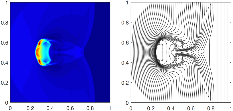
Figure 1: Example 2: the schlieren image of density (left), and the magnetic field lines (right) at $t=0.06$.

[Rotated shock tube problem]This is a rotated Riemann problem [38] with the left and right states respectively given by $(\rho,v_{\parallel},v_{\perp},u_{3},p,B_{\parallel},B_{\perp},B_{3})$ $=(1,10,0,0,20,5/\sqrt{4\pi},5/\sqrt{4\pi},0)$ and $(1,-10,0,0,1,5/\sqrt{4\pi},5/\sqrt{4\pi},0)$. The initial discontinuity is oblique to the Cartesian mesh and at an angle of $\varphi=45^{\circ}$ to the $\tt x$-axis. Similar to [40, 12, 32], the computational domain is taken as $[0,1]\times[0,2/N]$, and divided into a Cartesian mesh with $N\times 2$ square cells. The left and right boundaries are fixed according to the initial condition, and we stop the computation at $t=0.08\cos(\alpha)$ before the fast shocks reach the left and right boundaries. The shifted periodic type boundary conditions are used on the top and bottom of the domain as explained in [40]. We set $N=512$ and plot the numerical solution at the first row ($j=1$) of the physical mesh in Fig. 2. For comparisons, the non-rotated 1D solution on a fine mesh of 10000 cells is also displayed. Similar to the nonconservative eight-wave type schemes in [40, 12, 32], the proposed DG method also has the problem that the parallel component of the magnetic field, $B_{\parallel}$, which should be constant, shows a large error due to the nonconservative formulation. In our result, the $l^{\infty}$-norm of this error is about 0.0176, which is much less than that (about 0.2) in [12] obtained by a second-order finite volume scheme, and that (about 0.13) in [32] by a third-order DG scheme. The other quantities have good behavior in comparison with the reference solution and the results in [38].

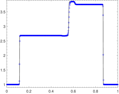
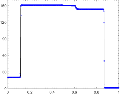
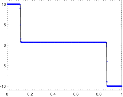
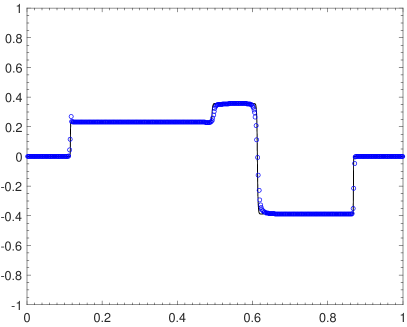
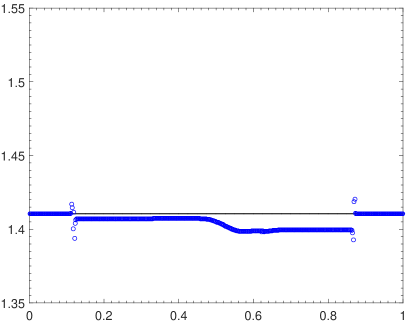
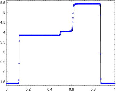
Figure 2: Example 1: Numerical solution of the 2D rotated shock tube problem obtained by the PP third-order DG method (“$\circ$”). For reference, the non-rotated 1D solution with 10000 cells is also plotted in solid lines. Top left: $\rho$; top right: $p$; middle left: $v_{\parallel}$; middle right: $v_{\perp}$; bottom left: $B_{\parallel}$; bottom right: $B_{\perp}$.

[Blast problems]MHD blast problem was first introduced by Balsara and Spicer in [5], and has become a standard test for 2D MHD codes. It describes the propagation of a circular strong fast magneto-sonic shock formulates and propagates into the ambient plasma with low plasma-beta ($\beta=2p/|{\bf B}|^{2}$). As $\beta$ is set lower, negative pressure is more likely to be produced in the numerical simulation and this problem becomes more challenging. Therefore, it is often used to check the robustness and PP property of MHD schemes, see e.g., [13, 15]. Initially, the computational domain $[-0.5,0.5]^{2}$ is filled with plasma at rest with the unit density and adiabatic index $\gamma=1.4$. The explosion zone $(r<0.1)$ is with a pressure of $p_{e}$, and the ambient medium $(r>0.1)$ has a lower pressure of $p_{a}$, where $r=\sqrt{{\tt x}^{2}+{\tt y}^{2}}$. We initialize the magnetic field in the $\tt x$-direction as $B_{a}$.

We first consider the same setup as in [5, 13], and take $p_{e}=10^{3}$, $p_{a}=0.1$ and $B_{a}=100/\sqrt{4\pi}$. The corresponding plasma-beta is very small and about $2.51\times 10^{-4}$. Fig. 3 shows the contour plots of density, pressure, velocity and magnetic pressure at $t=0.01$ computed by the PP third-order DG method with $320\times 320$ uniform cells. We can see that the outermost discontinuity in this expanding shell is a fast-shock which is only weakly compressive and energetically is dominated by the magnetic field. The density image clearly shows two dense shells which propagate parallel to the magnetic field. The outer wave of these shells is a slow-shock, and the inner is a contact discontinuity evolved from the initial interface which separates the initially hot, interior gas from the surrounding cool ambient medium [22]. Our results are highly in agreement with those displayed in [5, 30, 15], and the density profile is well captured with much less oscillations than those shown in [5, 15]. It is worth mentioning that the third-order DG method fails at $t\approx 2.85\times 10^{-4}$ if the PP limiting procedure is not employed to enforce the condition (25).

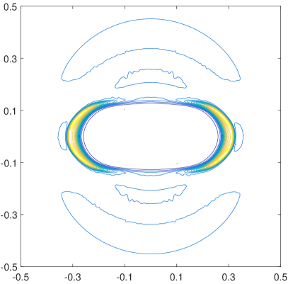
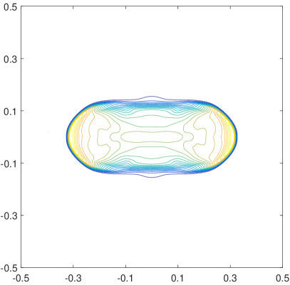
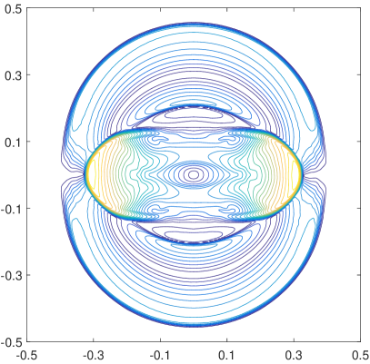
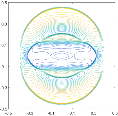
Figure 3: The first blast problem in Example 2: contour plots of density (top left), pressure (top right), velocity $|{\bf v}|$ (bottom left) and magnetic pressure (bottom right) at $t=0.01$.

To further demonstrate the robustness of the proposed PP DG method, we then test a more challenging case with larger initial jump in the pressure and much stronger magnetic field. More specifically, we set $p_{e}=10^{4}$, $p_{a}=0.1$ and $B_{a}=1000/\sqrt{4\pi}$. The corresponding plasma-beta is extremely small and about $2.51\times 10^{-6}$, which is $1\%$ of that in the above standard setup. To our best knowledge, such extreme blast problem is rarely considered in the literature. Fig. 4 displays the numerical results at $t=0.001$ obtained by the PP third-order DG method on the uniform mesh of $320\times 320$ cells. One can see that, as the magnetization is increased, the external fast shock becomes much weaker and is not visible in the counter plot of density. In this extreme test, it is also necessary to use the PP limiter to meet the condition (25), otherwise the DG method will fail at $t\approx 1.2\times 10^{-5}$ due to negative numerical pressure.

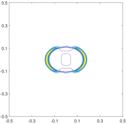
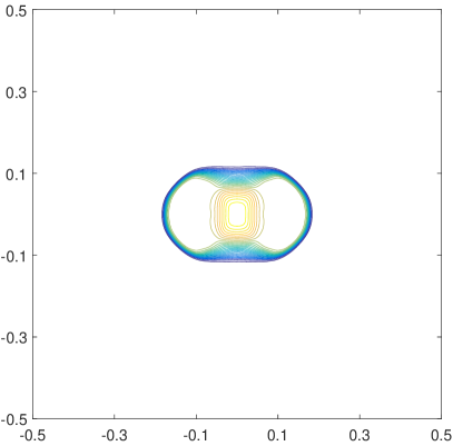
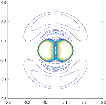
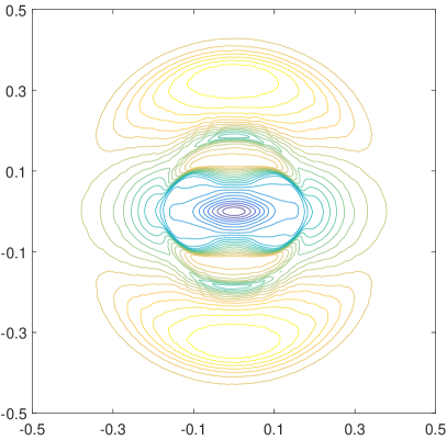
Figure 4: Same as Fig. 3 except for the second blast problem and $t=0.001$.

To justify that the CFL condition (27) is acceptable, we show the values of ${\vartheta_{\ell}}/{\alpha_{\ell,n}^{\tt LF}}$, $\ell=1,2,$ and $\theta$ in Fig. 5 for above two blast problems. We observe that, during the whole simulations, the ratios ${\vartheta_{\ell}}/{\alpha_{\ell,n}^{\tt LF}}$, $\ell=1,2,$ are very small, and $\theta$ is always larger than 0.98 and very close to 1. This is consistent with our analysis in Remark 3.6, and further confirms that $\theta$ in (27) does not cause strict restriction on the time step-sizes.

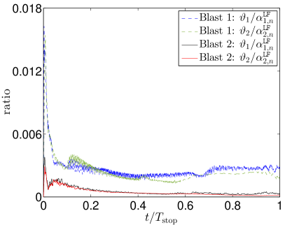
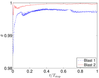
Figure 5: Example 2: ${\vartheta_{\ell}}/{\alpha_{\ell,n}^{\tt LF}}$ (left) and $\theta$ (right) for the two blast problems.

[Astrophysical jets]The last example is to simulate several astrophysical jets. If the jet speed is extremely high, the Mach number is very large and/or the magnetic field is exceedingly strong, then it is very challenging to successfully simulate such jet flows, see e.g., [55, 3, 45, 47]. Since the internal energy is very small compared to the huge kinetic energy and/or magnetic energy, negative pressure could easily appear in the numerical simulation. Moreover, there exist strong shock wave, shear flow and interface instabilities etc., in high-speed jet flows. Therefore, we have a strong motivation to use the PP high-order DG methods for this kind of problems.

Consider the Mach 800 dense jet in [3], and add a magnetic field to simulate the MHD jet flows. Initially, the physical domain $[-0.5,0.5]\times[0,1.5]$ is filled with a uniform static medium with density $0.1\gamma$ and unit pressure, and the adiabatic index $\gamma$ is set as $1.4$. Through the inlet part ($\left|{\tt x}\right|<0.05$) on the bottom boundary (${\tt y}=0$), a dense jet with speed $800$ is injected in the $\tt y$-direction with a density of $\gamma$ and a pressure equal to the ambient pressure. The fixed inflow beam condition is specified on the nozzle $\{{\tt y}=0,\left|{\tt x}\right|<0.05\}$, and the others are outflow boundary conditions. We initialize the magnetic field with magnitude $B_{a}$ along the $\tt y$-direction. With the magnetic field, this test becomes more extreme. As $B_{a}$ is set larger, the initial ambient magnetization becomes higher (plasma-beta becomes lower), and this problem becomes more challenging. Numerical experiments in [43] indicated that the locally divergence-free, conservative, third-order DG method with the PP limiter is not able to run this test with $B_{a}\geq\sqrt{200}$ due to the negative numerical pressure. In this test, we take the computational domain as $[0,0.5]\times[0,1.5]$ with the reflecting boundary condition specified at ${\tt x}=0$, and divide it into $200\times 600$ cells. Three configurations are considered:
(i) Moderately magnetized case: $B_{a}=\sqrt{200}$, corresponding plasma-beta $\beta_{a}=10^{-2}$.
(ii) Strongly magnetized case: $B_{a}=\sqrt{2000}$, corresponding plasma-beta $\beta_{a}=10^{-3}$.
(iii) Extremely strongly magnetized case: $B_{a}=\sqrt{20000}$, plasma-beta $\beta_{a}=10^{-4}$. Figs. 6 and 7 display, respectively, the schlieren images of density logarithm and pressure logarithm within the domain $[-0.5,0.5]\times[0,1.5]$. The “colormap” for plots of pressure logarithm is carefully chosen close to that in [3] for a sake of comparison, while for density logarithm we simply use the “jet colormap” predefined in MATLAB. As one can see, the flow structures in different magnetized cases are very different. The Mach shock wave at the jet head and the beam/cocoon interface are well captured, and the proposed PP DG method exhibits good performance and robustness in such extreme tests. And if the PP limiter is turned off, the simulation will break down after several time steps due to nonphysical numerical solutions.

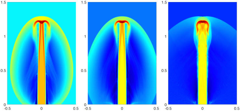
Figure 6: Example 5: Schlieren images of the density logarithm at $t=0.002$. From left to right: configurations (i) to (iii).

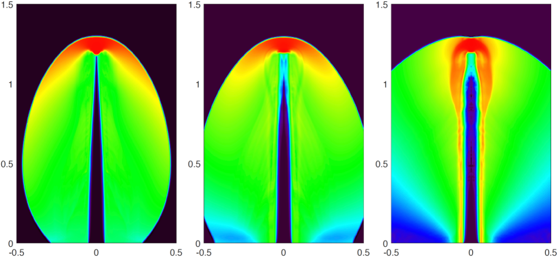
Figure 7: Same as Fig. 6 except for the schlieren images of pressure logarithm.

We now give more numerical evidences to support our analysis in Remark 3.6 about the CFL condition (27). The values of ${\vartheta_{\ell}}/{\alpha_{\ell,n}^{\tt LF}}$ and $\theta$ are shown in Fig. 8 for the challenging configuration (iii), while the results of configurations (i)–(ii) are similar and omitted. We see that, during the whole simulation, ${\vartheta_{\ell}}$ is much smaller than ${\alpha_{\ell,n}^{\tt LF}}$, $\ell=1,2,$ and $\theta$ is always very close to 1. This demonstrates, again, that $\theta$ in (27) does not cause strict restriction on the time step-sizes.

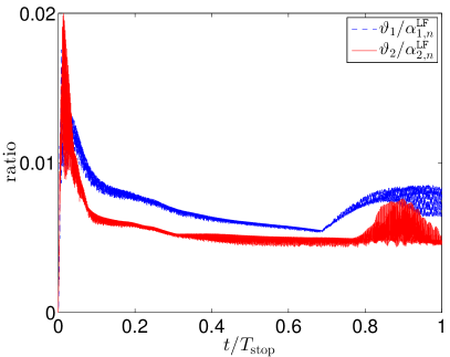
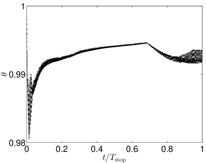
Figure 8: Example 2: ${\vartheta_{\ell}}/{\alpha_{\ell,n}^{\tt LF}}$ (left) and $\theta$ (right) for the jet problem in extremely strongly magnetized case.

5 Conclusions

We have constructed arbitrarily high-order accurate positivity-preserving (PP) discontinuous Galerkin (DG) schemes for multidimensional ideal compressible magnetohydrodynamics (MHD). It is based on the proposed locally divergence-free high-order DG schemes for the symmetrizable ideal MHD equations as the base schemes, the PP limiting procedure [13] to enforce the positivity of the DG solutions, and strong stability preserving methods [24] for time discretization. The significant innovation is that we discover and rigorously prove the PP property of the proposed DG schemes by using a novel equivalent form of the admissible state set and some very technical estimates. There are two features in our PP schemes: the locally divergence-free spatial discretization and the penalty-type terms discretized from the GP source term. The former leads to zero divergence within each cell, while the latter controls the divergence-error across the cell interfaces. Our PP analysis have showed that, thanks to these two features, the PP schemes are obtained without requiring the discrete divergence-free condition in [43], which was proposed for the conservative schemes without penalty-type terms. Several two-dimensional numerical experiments have confirmed the theoretical analysis, and demonstrated the accuracy, effectiveness and robustness of the proposed PP DG method.

The motivation of designing PP schemes based on the symmetrizable ideal MHD equations comes from an important observation: in the multidimensional cases, the exact solution of the conservative MHD equations (1) may fail to preserve the non-negativity of pressure if $\nabla\cdot{\bf B}\neq 0$, while it seems that the symmetrizable form (6) with an additional non-conservative source term does not suffer from this issue. There is still a conflict between the requirement of the non-conservative source term, and the conservation property of numerical schemes which is lost due to the source term. The extension of our PP methods to unstructured meshes is straightforward, but the proof of the PP property is much more technical and will be studied separately.

Appendix A Negative pressure may appear in the exact solution of conservative MHD system (1) if $\nabla\cdot{\bf B}\neq 0$

This appendix provides the evidence (not rigorous proof) on the claim that negative pressure may appear in the exact smooth solution of the conservative MHD system (1) if $\nabla\cdot{\bf B}\neq 0$.

Let focus on the ideal EOS (2) and $d=3$. We consider the following initial condition with nonzero divergence

(37) $$\rho({\bf x},0)=1,\qquad p({\bf x},0)=1-\exp(-|{\bf x}|^{2}),$$

$${\bf v}({\bf x},0)=(1,~{}1,~{}1),\qquad{\bf B}({\bf x},0)=(1+\delta B_{1},~{}1+\delta B_{2},~{}1+\delta B_{3}),$$

where ${\bf x}=(x_{1},x_{2},x_{3})$ and $\delta B_{i}=\frac{\epsilon}{3}\arctan x_{i}$, $i=1,2,3$, are small perturbations with $0<\epsilon\ll 1$. Since the initial data (37) is bounded and infinitely differentiable, it is reasonable to expect that, there exists a small time interval $[0,t_{*})$ such that the exact solution of the system (1) with the initial condition (37) is smooth for $t\in[0,t_{*})$. Under this assumption, one can study the initial time derivative of $p$ at ${\bf x}={\bf 0}$, although the analytical expression of the exact solution for $t>0$ is not available. For smooth solutions, it follows from (1) that

$$p_{t}+{\bf v}\cdot\nabla p+\gamma p\nabla\cdot{\bf v}+(\gamma-1)({\bf v}\cdot{\bf B})\nabla\cdot{\bf B}=0.$$

At $t=0$ and ${\bf x}={\bf 0}$, one has $\nabla p={\bf 0}$, $\nabla\cdot{\bf v}=0$ and $\nabla\cdot{\bf B}=\epsilon>0$, which yield

$$p_{t}({\bf 0},0)=-3(\gamma-1)\epsilon<0.$$

Note that $p({\bf 0},0)=0$. Thus there exists $t_{0}\in[0,t_{*})$ such that

$$p({\bf 0},t)<0,\quad\forall t\in(0,t_{0}).$$

We therefore have the reason to think that the non-negativity of pressure is not positively invariant for the conservative MHD system (1) if $\nabla\cdot{\bf B}\neq 0$. While the modified MHD system (6) may not suffer from this issue, because (6) implies

$$p_{t}+{\bf v}\cdot\nabla p+\gamma p\nabla\cdot{\bf v}=0.$$

Appendix B Two additional benchmark tests

The Orszag-Tang problem (see e.g., [28]) and rotor problem [5] are two benchmark tests widely simulated in the literature. Although not extreme, they are also tested by using the proposed PP third-order DG method to verify the effectiveness and high-resolution. Fig. 9 gives the contour plots of the computed density, which agree well with those in [5, 28].

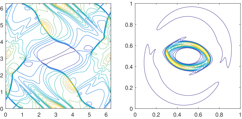
Figure 9: Numerical solutions of the Orszag-Tang problem with $200\times 200$ cells at $t=2$ (left) and the rotor problem with $400\times 400$ cells at $t=0.295$ (right).

References

- [1] J. Balbás and E. Tadmor, Nonoscillatory central schemes for one- and two-dimensional magnetohydrodynamics equations. II: High-order semidiscrete schemes, SIAM J. Sci. Comput., 28 (2006), pp. 533–560.
- [2] D. S. Balsara, Second-order-accurate schemes for magnetohydrodynamics with divergence-free reconstruction, Astrophys. J. Suppl. Ser., 151 (2004), pp. 149–184.
- [3] D. S. Balsara, Self-adjusting, positivity preserving high order schemes for hydrodynamics and magnetohydrodynamics, J. Comput. Phys., 231 (2012), pp. 7504–7517.
- [4] D. S. Balsara and D. Spicer, Maintaining pressure positivity in magnetohydrodynamic simulations, J. Comput. Phys., 148 (1999), pp. 133–148.
- [5] D. S. Balsara and D. Spicer, A staggered mesh algorithm using high order Godunov fluxes to ensure solenoidal magnetic fields in magnetohydrodynamic simulations, J. Comput. Phys., 149 (1999), pp. 270–292.
- [6] T. Barth, Numerical methods for gasdynamic systems on unstructured meshes, in An introduction to recent developments in theory and numerics for conservation laws, Springer, 1999, pp. 195–285.
- [7] T. Barth, On the role of involutions in the discontinuous Galerkin discretization of Maxwell and magnetohydrodynamic systems, in Compatible spatial discretizations, Springer, 2006, pp. 69–88.
- [8] F. Bouchut, C. Klingenberg, and K. Waagan, A multiwave approximate Riemann solver for ideal MHD based on relaxation. I: theoretical framework, Numer. Math., 108 (2007), pp. 7–42.
- [9] F. Bouchut, C. Klingenberg, and K. Waagan, A multiwave approximate Riemann solver for ideal MHD based on relaxation II: numerical implementation with 3 and 5 waves, Numer. Math., 115 (2010), pp. 647–679.
- [10] J. U. Brackbill and D. C. Barnes, The effect of nonzero on the numerical solution of the magnetodydrodynamic equations, J. Comput. Phys., 35 (1980), pp. 426–430.
- [11] P. Chandrashekar, P. Gallego, and C. Klingenberg, A Runge-Kutta discontinuous Galerkin scheme for the ideal magnetohydrodynamical model, in Springer Proceedings in Mathematics & Statistics: Theory, Numerics and Applications of Hyperbolic Problems, edited by C. Klingenberg and M. Westdickenberg, vol. 236, Springer, 2018.
- [12] P. Chandrashekar and C. Klingenberg, Entropy stable finite volume scheme for ideal compressible MHD on 2-D Cartesian meshes, SIAM J. Numer. Anal., 54 (2016), pp. 1313–1340.
- [13] Y. Cheng, F. Li, J. Qiu, and L. Xu, Positivity-preserving DG and central DG methods for ideal MHD equations, J. Comput. Phys., 238 (2013), pp. 255–280.
- [14] A. J. Christlieb, X. Feng, D. C. Seal, and Q. Tang, A high-order positivity-preserving single-stage single-step method for the ideal magnetohydrodynamic equations, J. Comput. Phys., 316 (2016), pp. 218–242.
- [15] A. J. Christlieb, Y. Liu, Q. Tang, and Z. Xu, Positivity-preserving finite difference weighted ENO schemes with constrained transport for ideal magnetohydrodynamic equations, SIAM J. Sci. Comput., 37 (2015), pp. A1825–A1845.
- [16] A. J. Christlieb, J. A. Rossmanith, and Q. Tang, Finite difference weighted essentially non-oscillatory schemes with constrained transport for ideal magnetohydrodynamics, J. Comput. Phys., 268 (2014), pp. 302–325.
- [17] B. Cockburn, S. Hou, and C.-W. Shu, The Runge-Kutta local projection discontinuous Galerkin finite element method for conservation laws. IV. the multidimensional case, Math. Comp., 54 (1990), pp. 545–581.
- [18] W. Dai and P. R. Woodward, A simple finite difference scheme for multidimensional magnetohydrodynamical equations, J. Comput. Phys., 142 (1998), pp. 331–369.
- [19] A. Dedner, F. Kemm, D. Kröner, C.-D. Munz, T. Schnitzer, and M. Wesenberg, Hyperbolic divergence cleaning for the MHD equations, J. Comput. Phys., 175 (2002), pp. 645–673.
- [20] P. J. Dellar, A note on magnetic monopoles and the one-dimensional mhd riemann problem, J. Comput. Phys., 172 (2001), pp. 392–398.
- [21] C. R. Evans and J. F. Hawley, Simulation of magnetohydrodynamic flows: a constrained transport method, Astrophys. J., 332 (1988), pp. 659–677.
- [22] T. A. Gardiner and J. M. Stone, An unsplit godunov method for ideal mhd via constrained transport, J. Comput. Phys., 205 (2005), pp. 509–539.
- [23] S. K. Godunov, Symmetric form of the equations of magnetohydrodynamics, Numerical Methods for Mechanics of Continuum Medium, 1 (1972), pp. 26–34.
- [24] S. Gottlieb, D. I. Ketcheson, and C.-W. Shu, High order strong stability preserving time discretizations, J. Sci. Comput., 38 (2009), pp. 251–289.
- [25] X. Y. Hu, N. A. Adams, and C.-W. Shu, Positivity-preserving method for high-order conservative schemes solving compressible Euler equations, J. Comput. Phys., 242 (2013), pp. 169–180.
- [26] P. Janhunen, A positive conservative method for magnetohydrodynamics based on HLL and Roe methods, J. Comput. Phys., 160 (2000), pp. 649–661.
- [27] L. Krivodonova, J. Xin, J.-F. Remacle, N. Chevaugeon, and J. E. Flaherty, Shock detection and limiting with discontinuous Galerkin methods for hyperbolic conservation laws, Appl. Numer. Math., 48 (2004), pp. 323–338.
- [28] F. Li and C.-W. Shu, Locally divergence-free discontinuous Galerkin methods for MHD equations, J. Sci. Comput., 22 (2005), pp. 413–442.
- [29] F. Li and L. Xu, Arbitrary order exactly divergence-free central discontinuous Galerkin methods for ideal MHD equations, J. Comput. Phys., 231 (2012), pp. 2655–2675.
- [30] F. Li, L. Xu, and S. Yakovlev, Central discontinuous Galerkin methods for ideal MHD equations with the exactly divergence-free magnetic field, J. Comput. Phys., 230 (2011), pp. 4828–4847.
- [31] C. Liang and Z. Xu, Parametrized maximum principle preserving flux limiters for high order schemes solving multi-dimensional scalar hyperbolic conservation laws, J. Sci. Comput., 58 (2014), pp. 41–60.
- [32] Y. Liu, C.-W. Shu, and M. Zhang, Entropy stable high order discontinuous Galerkin methods for ideal compressible MHD on structured meshes, J. Comput. Phys., 354 (2018), pp. 163–178.
- [33] P. Londrillo and L. Del Zanna, High-order upwind schemes for multidimensional magnetohydrodynamics, Astrophys. J., 530 (2000), pp. 508–524.
- [34] K. G. Powell, An approximate Riemann solver for magnetohydrodynamics (that works in more than one dimension), Tech. Report ICASE Report No. 94-24, NASA Langley, VA, 1994.
- [35] K. G. Powell, P. Roe, R. Myong, and T. Gombosi, An upwind scheme for magnetohydrodynamics, in 12th Computational Fluid Dynamics Conference, 1995, p. 1704.
- [36] J. Qiu and C.-W. Shu, Runge–Kutta discontinuous Galerkin method using WENO limiters, SIAM J. Sci. Comput., 26 (2005), pp. 907–929.
- [37] J. A. Rossmanith, An unstaggered, high-resolution constrained transport method for magnetohydrodynamic flows, SIAM J. Sci. Comput., 28 (2006), pp. 1766–1797.
- [38] D. Ryu, F. Miniati, T. Jones, and A. Frank, A divergence-free upwind code for multidimensional magnetohydrodynamic flows, Astrophys. J., 509 (1998), pp. 244–255.
- [39] M. Torrilhon, Locally divergence-preserving upwind finite volume schemes for magnetohydrodynamic equations, SIAM J. Sci. Comput., 26 (2005), pp. 1166–1191.
- [40] G. Tóth, The constraint in shock-capturing magnetohydrodynamics codes, J. Comput. Phys., 161 (2000), pp. 605–652.
- [41] K. Waagan, A positive MUSCL-Hancock scheme for ideal magnetohydrodynamics, J. Comput. Phys., 228 (2009), pp. 8609–8626.
- [42] K. Waagan, C. Federrath, and C. Klingenberg, A robust numerical scheme for highly compressible magnetohydrodynamics: Nonlinear stability, implementation and tests, J. Comput. Phys., 230 (2011), pp. 3331–3351.
- [43] K. Wu, Positivity-preserving analysis of numerical schemes for ideal magnetohydrodynamics, SIAM J. Numer. Anal., accepted. Available at arXiv:1802.02278.
- [44] K. Wu, Design of provably physical-constraint-preserving methods for general relativistic hydrodynamics, Phys. Rev. D, 95 (2017), 103001.
- [45] K. Wu and H. Tang, High-order accurate physical-constraints-preserving finite difference WENO schemes for special relativistic hydrodynamics, J. Comput. Phys., 298 (2015), pp. 539–564.
- [46] K. Wu and H. Tang, Admissible states and physical-constraints-preserving schemes for relativistic magnetohydrodynamic equations, Math. Models Methods Appl. Sci., 27 (2017), pp. 1871–1928.
- [47] K. Wu and H. Tang, Physical-constraint-preserving central discontinuous Galerkin methods for special relativistic hydrodynamics with a general equation of state, Astrophys. J. Suppl. Ser., 228 (2017), 3.
- [48] Y. Xing, X. Zhang, and C.-W. Shu, Positivity-preserving high order well-balanced discontinuous Galerkin methods for the shallow water equations, Adv. Water Res., 33 (2010), pp. 1476–1493.
- [49] T. Xiong, J.-M. Qiu, and Z. Xu, Parametrized positivity preserving flux limiters for the high order finite difference WENO scheme solving compressible Euler equations, J. Sci. Comput., 67 (2016), pp. 1066–1088.
- [50] Z. Xu, Parametrized maximum principle preserving flux limiters for high order schemes solving hyperbolic conservation laws: one-dimensional scalar problem, Math. Comp., 83 (2014), pp. 2213–2238.
- [51] Z. Xu and X. Zhang, Bound-preserving high order schemes, in Handbook of Numerical Methods for Hyperbolic Problems: Applied and Modern Issues, edited by R. Abgrall and C.-W. Shu, vol. 18, North-Holland, Amsterdam, 2017, Elsevier.
- [52] S. Yakovlev, L. Xu, and F. Li, Locally divergence-free central discontinuous Galerkin methods for ideal MHD equations, J. Comput. Sci., 4 (2013), pp. 80–91.
- [53] X. Zhang, On positivity-preserving high order discontinuous Galerkin schemes for compressible Navier-Stokes equations, J. Comput. Phys., 328 (2017), pp. 301–343.
- [54] X. Zhang and C.-W. Shu, On maximum-principle-satisfying high order schemes for scalar conservation laws, J. Comput. Phys., 229 (2010), pp. 3091–3120.
- [55] X. Zhang and C.-W. Shu, On positivity-preserving high order discontinuous Galerkin schemes for compressible Euler equations on rectangular meshes, J. Comput. Phys., 229 (2010), pp. 8918–8934.
- [56] X. Zhang and C.-W. Shu, Maximum-principle-satisfying and positivity-preserving high-order schemes for conservation laws: survey and new developments, Proc. R. Soc. A, 467 (2011), pp. 2752–2776.
- [57] X. Zhang and C.-W. Shu, Positivity-preserving high order discontinuous Galerkin schemes for compressible Euler equations with source terms, J. Comput. Phys., 230 (2011), pp. 1238–1248.
- [58] J. Zhao and H. Tang, Runge-Kutta discontinuous Galerkin methods for the special relativistic magnetohydrodynamics, J. Comput. Phys., 343 (2017), pp. 33–72.