Automatic Identification of Twin Zygosity in Resting-State Functional MRI

Abstract

A key strength of twin studies arises from the fact that there are two types of twins, monozygotic and dizygotic, that share differing amounts of genetic information. Accurate differentiation of twin types allows efficient inference on genetic influences in a population. However, identification of zygosity is often prone to errors without genotying. In this study, we propose a novel pairwise feature representation to classify the zygosity of twin pairs of resting state functional magnetic resonance images (rs-fMRI). For this, we project an fMRI signal to a set of basis functions and use the projection coefficients as the compact and discriminative feature representation of noisy fMRI. We encode the relationship between twins as the correlation between the new feature representations across brain regions. We employ hill climbing variable selection to identify brain regions that are the most genetically affected. The proposed framework was applied to 208 twin pairs and achieved 94.19% classification accuracy in automatically identifying the zygosity of paired images.

Keywords: Twin resting-state fMRI, variable selection method, heritability

1 Introduction

The extent by which genetic factors shape brain function is still largely unknown. Twin brain imaging studies provide a valuable information for quantifying such extend in-vivo. The power of twin studies arises from the fact that there are only two types of twins, identical (or monozygotic, MZ) and fraternal (or dizygotic, DZ), that share differing amounts of genetic information. In average, MZ twins are expected to share 100% of genes, and DZ twins are expected to share only 50% of genes (Neale & Cardon, 2013). By comparing the similarity between MZ and DZ twins, we can quantify the genetic influence in a population.

Unfortunately, zygosity identification of twins is prone to errors even for the obstetricians delivering babies. As many as twenty percent of all twin births are misidentified according to Minnesota Center for Twin and Family Research (2007). Recently, a dataset containing high-quality brain images of twins has become available through the Human Connectome Project (http://www.humanconnectome.org, HCP). In HCP, 35 pairs originally self-reported as DZ twins were later confirmed to be MZ twins after genotyping. Out of 243 twin pairs, this produces the error rate of 14%. Such a high misclassification rate most likely contributed significantly to mislabeling in many past twin studies without genotyping. In this paper, we explore the feasibility of developing a reliable pipeline for automatic zygosity classification without genotyping.

The significance of genetic contribution in twin studies has been reliably shown for a wide range of functional brain imaging studies  (Jansen et al., 2015; Richmond et al., 2016), including heritability of neural activation during simple visuomotor task (Park et al., 2012), calculation (Pinel & Dehaene, 2013), oral reading recognition and picture vocabulary comprehension (Babajani-Feremi, 2017), estimating genetic contribution to brain activation in neural networks supporting working memory tasks (Karlsgodt et al., 2007; Blokland et al., 2008, 2011; Koten et al., 2009). Several studies involving resting state functional MRI have also discovered significant genetic contributions to functional network connectivity architecture of the human brain (Glahn et al., 2010; Fornito et al., 2011; van den Heuvel et al., 2013; Gao et al., 2014; Yang et al., 2016). These studies mainly utilized the concept of functional connectivity to infer the heritability of brain regions using the Pearson’s correlation coefficient between blood-oxygen-level dependent (BOLD) contrasts. Inference on a region’s heritability is then typically performed using the ACE model, which factors all differences in population to three components: additive genetic effects, common and unique environments (Maes, 2005; Falconer et al., 1996). In this study, we design a new framework to determine heritability of brain regions in a model-free setting.

The idea of using functional MRI data for individual identification and prediction has been successfully applied in several recent studies. For example, Miranda-Dominguez et al. (2014) described a model-based approach capable of identifying a functional fingerprint, ’connectotype’, in individual participants through predicting resting state brain activity of each ROI as the weighted sum of all other ROIs. Finn et al. (2015) investigated this further and showed that individual connectotype of brain activity is preserved not only across scan sessions but also between task and rest conditions. Smith et al. (2015) used Canonical Correlation Analysis (CCA) to demonstrate a strong covariation link between brain connectivity and demographics, psychometrics and behavioral subject measures. However, these approaches are not directly applicable in their original form to our specific problem of zygosity classification. In these papers, the main aim is to accurately distinguish each subject from the rest of population, while our goal is a more general classification scheme of classifying paired images into two categories.

In the past, machine learning methods such as artificial neural networks (ANN), support vector machines, $k$-nearest neighbor, Gaussian naïve Bayes and fuzzy classifiers (LaConte et al., 2005; Singh et al., 2007; Pereira et al., 2009; Peltier et al., 2009; Vergun et al., 2013; Wang et al., 2014; Honorio, 2015; Wang et al., 2017) have been used to analyze fMRI data. However, none of them have been used for classifying paired twin images. It is unclear how to apply existing classifiers to twin rs-fMRI. For the first time, we propose a unified classification framework that automatically determines the zygosity of a twin-pair using resting-state fMRI and identifies specific brain regions with significant genetic influence. The framework combines the algebraic representation of fMRI time series at the voxel-level with the sparse version of a multi-layer artificial neural network.

For our non-trivial classification problem setting, where each classification identity is represented by a pair of twin images, a special type of neural network is required, specifically designed to process paired data through a comparative analysis. This type of neural networks is related to siamese neural network (SNN) (Bromley et al., 1994; Zagoruyko & Komodakis, 2015) and has recently gained interest in the medical imaging community (Kouw et al., 2017; Ktena et al., 2017; Wang & Yang, 2018; Ktena et al., 2018). One of the main features of SNN is the ability to learn the suitable embedding space of the original data, that is usually composed of highly abstract and semantic information. The drawback of SNN is that it is difficult to obtain a meaningful biological interpretation of this abstract embedding. Instead of learning paired representation through a blackbox approach like SNN, we propose to introduce a parametric algebraic framework that provides an easy-to-comprehend twin representation. In our framework, a new compact feature representation for the fMRI signal at each voxel is obtained using the cosine series representation (CSR). The correlation between twins at voxel level computed using CSR features is feed into in a two-layer ANN. Currently, the majority of brain image analysis studies compute correlation directly from resting state fMRI signal (Biswal et al., 1997; Peltier et al., 2005; Rogers et al., 2007; Liang et al., 2012; Finn et al., 2015; Joshi et al., 2017). In contrast, CSR compactly represent fMRI components into frequency components, which provides a superior performance with respect to the classification accuracy. Our framework can further incorporate a variable selection procedure and able to localize the brain regions that are most heritable.

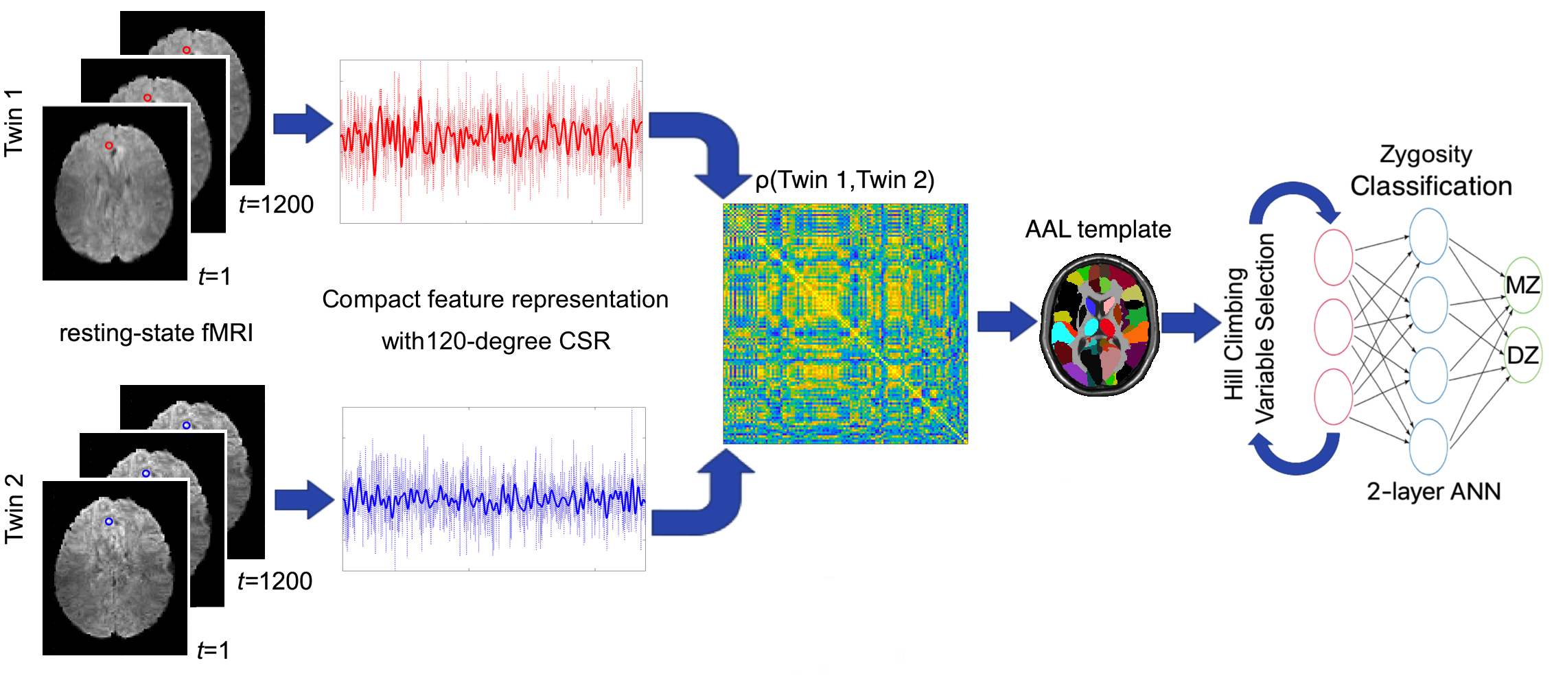
Figure 1: Pipeline of the proposed framework. The 120-degree cosine series representations are displayed as the solid lines. Twin correlation between CSR coefficients are computed at each voxel. We use AAL brain atlas to parcellate the voxel-level correlations into 116 region-level correlations. The resulting vectors of 116 twin correlations are feed into a two-layer feedforward neural network to automatically determine zygosity of twin pair.

The main contributions of the paper are: (1) we introduce a new feature representation in characterizing twin-wise relationships in the whole brain that substantially improves classification performance; (2) for the first time, we develop a highly reliable zygosity classification scheme without genotyping with $94.19\%$ accuracy; (3) we propose a principled way of determining the most genetically heritable regions in the brain through the classification scheme.

The proposed framework is applied to HCP, one of the largest publicly available twin datasets, that contains rs-fMRI data of 131 MZ and 77 DZ twin pairs.

2 Material and Methods

2.1 Dataset

We use resting-state fMRI scans collected as part of the Washington University-Minnesota Consortium Human Connectome Project (HCP)  (Van Essen & Ugurbil, 2012; Van Essen et al., 2012, 2013). All participants gave informed consent. The HCP dataset provides information about both self-reported and genotyping-verified zygosity of each twin pair. Subjects’ genotyping data has been derived from blood or saliva based genytyping (WU-Minn HCP Consortium, 2018). As our interest lies in identifying the zygosity of twin pairs, we only investigated fMRI scans of genetically confirmed 149 monozygotic (MZ) and 94 same-sex dizygotic (DZ) twins. The zygosity status has not been confirmed for 19 MZ and 9 DZ twin pairs via genotyping. Out of genetically-verified 243 pairs, we excluded 35 twins with missing functional MRI data resulting in the final dataset consisting of 131 MZ (age $29.3\pm 3.3$, 56M/75F) and 77 DZ twin pairs (age $29.1\pm 3.5$, 30M/47F). Demographic details of twin pairs are summarized in Table 1.

Table 1: Demographic data of twin groups

Twin group	Sample size	Sex (M/F)	Age
MZ	131	56/75	$29.3\pm 3.3$
DZ	77	30/47	$29.1\pm 3.5$

MZ: monozygotic twins, DZ: dizygotic twins. Age is displayed in years as Mean$\pm$SD.

All subjects were scanned on a customized Siemens 3T Connectome Skyra scanner housed at Washington University in St. Louis, using a standard 32-channel Siemens receive head coil and a customized SC72 gradient insert and a customized body transmitter coil with 56 cm bore size. Resting-state functional MRI were collected over 14 minutes and 33 seconds using a gradient-echo-planar imaging (EPI) sequence with multiband factor 8, time repetition (TR) 720 ms, time echo (TE) 33.1 ms, flip angle $52^{\circ}$, $104\times 90$ (RO$\times$PE) matrix size, 72 slices, 2 mm isotropic voxels, and 1200 time points. During each scanning participants were at rest with eyes open with relaxed fixation on a projected bright cross-hair on a dark background and presented in a darkened room (WU-Minn HCP Consortium, 2018).

We used fMRI scans that undergone spatial (Glasser et al., 2013) and temporal (Smith et al., 2013) preprocessing correcting including : removal of spatial distortions, realigning volumes to compensate for subject motion, registering the fMRI data to the structural MNI template, minimal highpass temporal frequency filtering, independent component analysis (ICA)-based artifact removal. The resulting volumetric data contains resting-state functional time series with $91\times 109\times 91=902629$ 2-mm isotropic voxels at 1200 imaging volumes.

2.2 Cosine Series Representation

Given the fMRI time series $\zeta(\nu,t)$ at the voxel $\nu$ and time $t$, we scale it to the unit interval $[0,1]$, ans then subtract its mean over time $\int_{0}^{1}\zeta(\nu,t)\;dt$. The scaled and translated time series is subsequently represented as

$$\zeta(\nu,t)=\sum_{l=0}^{k}c_{l,\nu}\psi_{l}(t),\;t\in[0,1],$$

where $\psi_{0}(t)=1,\psi_{l}(t)=\sqrt{2}\cos(l\pi t)$ are orthonormal cosine basis functions satisfying

$$\big{\langle}\psi_{l},\psi_{m}\big{\rangle}=\int_{0}^{1}\psi_{l}(t)\psi_{m}(t)dt=\delta_{lm}$$

where $\delta_{lm}$ is the Kronecker’s delta. The coefficients $c_{l,\nu}$ are estimated in the least squares fashion, i.e.,

$$c_{l,\nu}=\operatorname*{arg\,min}_{c_{l,\nu}\in\mathbb{R}}\Big{\|}\sum_{l=0}^{k}c_{l,\nu}\psi_{l}(t)-\zeta(\nu,t)\Big{\|}^{2}.$$

For our study, the expansion degree $k=119$ is used such that fMRI is compressed into 10% of its original data size. The choice of $k=119$ expansion increases the signal-to-noise ratio (SNR) as measured by the ratio of variabilities by 73% in average over all voxels in 416 subjects, i.e., SNR = 1.73. The resulting coefficient vector ${\bf c}_{\nu}=(c_{0,\nu},c_{1,\nu},\cdots,c_{k,\nu})$ is then used to represent the fMRI in voxel $v$. The CSR for multiple time series can be computed by solving for $p=1200$ time points

$$\underbrace{\begin{pmatrix}\zeta(\nu_{1},t_{1})&\cdots&\zeta(\nu_{n},t_{1})\\ \vdots&\zeta(\nu_{i},t_{j})&\vdots\\ \zeta(\nu_{1},t_{p})&\cdots&\zeta(\nu_{n},t_{p})\end{pmatrix}}_{\mathrm{Z}_{p\times n}}=\underbrace{\begin{pmatrix}\psi_{0}(t_{1})&\cdots&\psi_{k}(t_{1})\\ \vdots&\psi_{l}(t_{j})&\vdots\\ \psi_{0}(t_{p})&\cdots&\psi_{k}(t_{p})\end{pmatrix}}_{\Psi_{p\times k}}\underbrace{\begin{pmatrix}c_{0,\nu_{1}}&\cdots&c_{0,\nu_{n}}\\ \vdots&c_{l,\nu_{i}}&\vdots\\ c_{k,\nu_{1}}&\cdots&c_{k,\nu_{n}}\end{pmatrix}}_{\mathrm{C}_{k\times n}}.$$

The least squares estimate of $C$ is given by

$$\widehat{\mathrm{C}}=(\Psi^{T}\Psi)^{-1}\Psi^{T}\mathrm{Z}.$$

2.3 Correlations between CSR

Consider the CSR of fMRI obtained from the first and second subjects in a twin pair at the same voxel $\nu$ (Figure 1)

$$\zeta(\nu,t)=\sum_{l=0}^{k}\zeta_{l}\psi_{l}(t),\quad\eta(\nu,t)=\sum_{l=0}^{k}\eta_{j}\psi_{l}(t),$$

where

$$\zeta_{l}=\big{\langle}\zeta,\psi_{l}\big{\rangle},\quad\eta_{l}=\big{\langle}\eta,\psi_{l}\big{\rangle}$$

are CSR coefficients. Since fMRI was normalized with respect to the mean over time, the variance of $\zeta(\nu,t)$ and $\eta(\nu,t)$ is given by

$$\sigma^{2}\!\>\zeta=\int_{0}^{1}\zeta^{2}(\nu,t)\!\>dt,\quad\sigma^{2}\!\>\eta=\int_{0}^{1}\eta^{2}(\nu,t)\!\>dt.$$

The correlation $\rho(\zeta,\eta)$ between $\zeta(\nu,t)$ and $\eta(\nu,t)$ is then given by

$$\rho(\zeta,\eta)=\frac{\int_{0}^{1}\zeta(\nu,t)\!\>\eta(\nu,t)\!\>dt}{\sigma\zeta(\nu,t)\cdot\sigma\eta(\nu,t)}=\frac{\sum_{l_{1}=0}^{k}\sum_{l_{2}=0}^{k}\zeta_{l_{1}}\eta_{l_{2}}\big{\langle}\psi_{l_{1}},\psi_{l_{2}}\big{\rangle}}{\big{[}\sum_{l=0}^{k}\zeta_{l}^{2}\big{]}^{\frac{1}{2}}\cdot\big{[}\sum_{l=0}^{k}\eta_{l}^{2}\big{]}^{\frac{1}{2}}}=\boldsymbol{\zeta}^{T}\boldsymbol{\eta},$$

where

$$\boldsymbol{\zeta}=\frac{(\zeta_{1,\nu},\cdots,\zeta_{k,\nu})^{T}}{\big{[}\sum_{l=0}^{k}\zeta_{l,\nu}^{2}\big{]}^{1/2}},\quad\boldsymbol{\eta}=\frac{(\eta_{1,\nu},\cdots,\eta_{k,\nu})^{T}}{\big{[}\sum_{l=0}^{k}\eta_{l,\nu}^{2}\big{]}^{1/2}}$$

are vectors of cosine series representation coefficients.

Note $\rho$ is the correlation of low frequency components of time series in the frequency domain. In task-related twin fMRI studies, correlation between twins can be computed in a straightforward manner in the temporal domain because the timing of neuronal activation is comparable across subjects due to the exterior task. However, in the resting-state fMRI there is no external anchor that will lock brain activation of twin subjects across time. Thus, we utilize cosine series representation of fMRI signals to compute correlation between twin subjects in the frequency domain. Similar approaches were used in (Curtis et al., 2005; Ombao & Van Bellegem, 2008), where frequency components of signals are correlated using coherence.

2.4 Twin Classification with Artificial Neural Network

Given paired twin images represented as a vector of region-level correlations between CSR coefficients of the original twin fMRI, we use ANN to identify if they belong to a pair of MZ or DZ twins. Since we classify the relationship between paired images, this is not a traditional binary classification problem often performed in brain imaging. We use a two-layer feed-forward ANN, with 200 sigmoid hidden and 1 softmax output neurons to classify the vectors of average correlations (Møller, 1993).

We further employ AAL parcellation to compute pairwise twin correlation at region level by averaging across voxels in each parcellation. Since we cannot average correlations by taking the arithmetic mean without biasing, we transform correlations using the Fisher $z$-transform first:

$$z=F(\rho)=\frac{1}{2}\ln{\frac{1+\rho}{1-\rho}}.$$

Then, Fisher transformed correlations are averaged and back projected via the inverse transform (Vrbik, 2005). The result is the vector of 116 twin correlations that are feed into the neural network.

Due to possible dependencies between AAL regions, some AAL regions contribute differently to the classification accuracy. We introduce an $\ell_{1}$-regularization term to the loss function:

$$\mathcal{L}(w)=-\frac{1}{N}\sum_{i=1}^{N}[t_{i}\log y_{i}+(1-t_{i})\log(1-y_{i})]+\lambda\sum_{\kappa=1}^{M}\|w_{\kappa}\|_{1},$$ (1)

where $t_{i}$ is the class label for the $i$-th twin pair (’1’ for MZ twin pair, ’0’ for DZ twin pair), $y_{i}$ is the predicted class label for the $i$-th twin pair, $N$ is the number of twin pairs in the training set, $w_{\kappa}$ is a vector of weights corresponding to a $\kappa$-th AAL region, and $M=116$ is the number of regions of interest. Adding regularization to the ANN prevent model overfitting. Further, $\ell_{1}$-regularization increases the model’s sparsity by penalizing large weights between neurons, thus implicitly removing unimportant features from the model. In brain imaging, regularization is mainly used for segmentation tasks and feature selection (Liu et al., 2018; Sanroma et al., 2018; Guo et al., 2017; Wang et al., 2015). However, here we use it to remove brain regions, whose contribution to zygosity identification can be neglected.

Solving a binary classification problem with artificial neural nets is equivalent to solving a regression problem with subsequent application of the thresholding rule:

$$y_{i}=\begin{cases}1\quad\text{if}\;\;o_{i}\geq\theta,\\ 0\quad\text{if}\;\;o_{i}<\theta,\end{cases}$$ (2)

where $o_{i}$ is numerical output of the neural network for the $i$-th pair of twins, and $\theta$ is the discrimination threshold.

Given a binary classification problem, we take the fMRI data from pairs of MZ twins belonging to the positive class ($t_{i}=1$) and the fMRI data from pairs of DZ twins belonging to the negative class ($t_{i}=0$). We use the holdout method to split dataset randomly into training (70% of the data), validation (15%) and test (15%) subsets. The validation dataset is used to avoid overtraining of the model, and to fine tune hyperparameters of the neural network, e.g., the number of hidden neurons and discrimination threshold $\theta$. Splitting data into training, validation and test subsets in the proportion of 70:15:15 is considered as the gold standard (Hagan et al., 2014). We trained 1000 independently initialized models without preserved class ratio and average performance across them. We employ classification accuracy, false-positive rate (FPR) and false-negative rate (FNR) to measure the performance of the proposed framework.

2.5 Boosting Accuracy with Variable Selection

To infer the contribution of different regions to classification accuracy of the model, we further implemented a hill climbing variable selection procedure considering each AAL parcellation as a variable (Russell & Norvig, 2003). Hill climbing is an iterative optimization technique that attempts to find a better solution by incrementally changing a single element of the solution. If the change produces a better solution, an incremental change is made to the new solution, repeating until no further improvements can be found. With the application to variable selection, we implement hill climbing procedure as follows.

We start with the empty variable space and a pool of candidate variables. At each iteration, we test candidate variables by picking one variable at a time, adding it to the model and estimating the performance of the model. When all candidate variables are tested, the variable that provides the best performance, with respect to classification accuracy, false positive rate (FPR) and false negative rate (FNR), is removed from the pool of candidates and added to the variable space of the model. Variables are ranked with respect to classification accuracy. We continue the process iteratively until all variables are added to the model. We rank AAL regions with respect to the classification accuracy they provide to the model based on iterations, when the corresponding variables are added to the variable space. The higher the region is ranked by hill climbing, the more the region is affected by the genetic effect.

3 Simulation Study

Table 2: Simulation results

Study	Accuracy (%)	FPR (%)	FNR (%)
Study 1	48.63($\pm$12.37)	50.64($\pm$24.24)	49.98($\pm$24.04)
Study 2	79.79($\pm$10.66)	24.65($\pm$14.66)	13.51($\pm$14.43)
Study 3a	81.88($\pm$10.43)	23.02($\pm$16.84)	12.98($\pm$14.40)
Study 3b	87.65($\pm$8.11)	16.93($\pm$13.98)	7.24($\pm$9.78)

FPR (false-positive rate), FNR (false-negative rate) and overall classification accuracy are provided with standard deviation. Study 1: No twin difference. Study 2: Twin difference. For Study 3: Differential twin difference, we present classification performance both not employing (Study 3a) and employing (Study 3b) variable selection procedure.

We validated the proposed twin classification framework using simulation studies with known ground truth. We first generated ground truth data that represents the underlying resting-state functional MRI signals from $M=5$ distinct brain regions of interest using degree 5 CSR. The CSR coefficients are

$$\mathbf{c_{1}}=\mathbf{c_{2}}=\mathbf{c_{3}}=\mathbf{c_{4}}=\mathbf{c_{5}}=\Big{[}1,\frac{1}{2},\frac{1}{3},\frac{1}{4},\frac{1}{5}\Big{]}^{T}.$$

We generate twin data in $\kappa$-th region using the mixed-effect model:

$$\begin{gathered}\zeta_{\kappa,i}=\mathbf{c_{\kappa}}+\alpha_{\kappa,Twin}+\beta_{\kappa,i},\\ \eta_{\kappa,i}=\mathbf{c_{\kappa}}+\alpha_{\kappa,Twin}+\beta_{\kappa,i},\end{gathered}$$ (3)

where $\zeta_{\kappa,i}$ is the vector of CSR coefficients of the first twin in the $i$-th pair, $\eta_{\kappa,i}$ is the vector of CSR coefficients of the second twin in the $i$-th pair, $\alpha_{\kappa,Twin}$ is a twin-level noise distributed as $N(0,\sigma_{\kappa,Twin}^{2})$ and $\beta_{\kappa,i}$ is an individual-level noise distributed as $N(0,\sigma_{\kappa,Ind}^{2})$. After the synthetic twin data is generated, we applied the proposed ANN framework: compute correlations between twins, train ANN to classify zygosity of twin pairs, and estimate the extent by which regions of interest are affected by the genetic effects using hill climbing variable selection procedure.

We perform three different simulation studies using the same ground truth coefficients $\mathbf{c_{\kappa}}$ and individual-level variance $\sigma_{\kappa,Ind}^{2}=0.25^{2}$, but different twin-level variances, $\sigma_{\kappa,MZ}^{2},\,\sigma^{2}_{\kappa,DZ}$ depending on the zygosity of twin pairs. In all three simulations, we generate 50 MZ pairs and 50 DZ pairs. To obtain stable results we repeated the simulation 1000 times and the average results are reported. The simulation results are processed simultaneously by logistic regression model and our classification framework and averaged results are summarized in Table 2 and Figure 2.

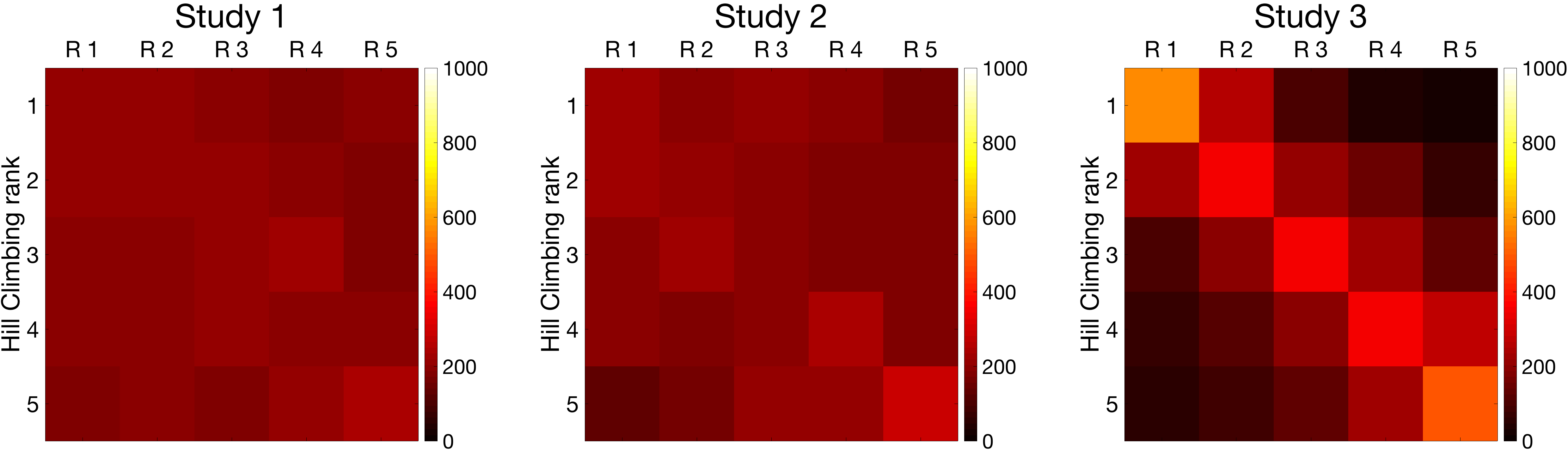
Figure 2: Results of hill climbing variable selection for three simulation studies. For each region of interest $\kappa$, The value at the intersection of $\kappa$-th column and $i$-th row represents how often this regions has been selected at the $i$-th iteration of the hill climbing variable selection procedure.

Study 1: No twin difference

We tested if the method is detecting any false positive when there is no twin difference. By letting the DZ-variability equal the MZ-variability

$$\sigma_{\kappa,DZ}^{2}=\sigma_{\kappa,MZ}^{2}=\sigma_{\kappa,Ind}^{2},$$

we are generating twin data without any DZ- and MZ-twin difference. The classification accuracy for the proposed framework is $48.63\pm 12.37\%$ indicating we are not falsely classifying the zygosity.

Study 2: Twin difference

We forced all 5 regions to be equally highly heritable. We achieve this by simulating MZ twin data with smaller twin-level variance compared to DZ twin data:

$$\sigma_{\kappa,MZ}^{2}=\sigma_{\kappa,Ind}^{2},\,\sigma_{\kappa,DZ}^{2}=2^{2}\sigma_{\kappa,Ind}^{2},$$

The classification accuracy for the proposed framework is $79.79\pm 10.66\%$ indicating we are classifying zygosity.

Study 3: Differential twin difference

We forced 5 regions to have gradually decreasing heritability:

$$\sigma_{\kappa,MZ}^{2}=\sigma_{\kappa,Ind}^{2},\,\sigma_{\kappa,DZ}^{2}=h_{\kappa}^{2}\sigma_{\kappa,Ind}^{2},$$

where $\{h_{\kappa}\}=\{3,2.5,2,1.5,1\}$ is a sequence of gradually decreasing numbers that control heritability of each $\kappa$-th region of interest. The classification accuracy for the proposed framework in Study 3 without hill climbing is $81.88\pm 10.43\%$. When utilizing hill climbing, the accuracy increased to $87.65\pm 8.11\%$ indicating we are gaining advantage by employing variable selection in case of unequal heritability across regions. ROI rankings provided by hill climbing correspond to the gradually decreasing heritability of regions (Figure 2).

4 Results

The proposed ANN framework was applied to the HCP rs-fMRI data from 208 twin pairs. The classification performance is reported in Table 3. We achieved $54.15(\pm 9.24)\%$ accuracy when original rs-fMRI were used in computing twin correlations. The use of CSR improved the accuracy significantly and achieved $79.93(\pm 7.59)\%$ accuracy with $36.98(\pm 17.29)\%$ false-positive rate and $9.99(\pm 6.79)\%$ false-negative rate.

Table 3: Performance of the proposed classification pipeline at different stages

Method	Accuracy (%)	FPR (%)	FNR (%)
ANN w/o CSR	54.15($\pm$9.24)	74.67($\pm$18.74)	28.36($\pm$17.09)
ANN w/ CSR	79.93($\pm$7.59)	36.98($\pm$17.29)	9.99($\pm$6.79)
ANN + Hill climbing	94.19($\pm$3.53)	9.54($\pm$6.87)	3.69($\pm$3.47)
Logistic regression	47.99($\pm$3.32)	61.62($\pm$5.56)	38.24($\pm$4.14)

FPR: false-positive rate, FNR: false-negative rate. Overall classification accuracy, false-positive rate and false-negative rate are provided for the test subset in percentages with standard deviations.

4.1 Detecting the Most Heritable Regions

Hill climbing was used on ANN classification to further identify the most heritable brain regions and improve the performance. In hill climbing, each variable represents the average correlation between twins in a single AAL parcellation. Figure 3 illustrates the results of the variable selection procedure accumulated across 1000 independently initialized models. Figure 3 displays how often hill climbing selects a certain variable at a given iteration. Based on the results of hill climbing, we infer the extent each ROI contributes to the zygosity classification. We estimate the contribution of $\kappa$-th AAL parcellation using the following criterion

$$\mathcal{J}(\kappa)=\sum_{i=1}^{M}\frac{\gamma(\kappa,i)}{i},$$

where $\gamma(\kappa,i)$ is the number of times when the brain region $\kappa$ has been added to the variable space at the $i$-th iteration, and $M$ is the total number of the variables ($M=116$ in this study). Regions that have been selected by hill climbing at least once across all models are marked with bold font, and the most important $85$-th percentile regions are marked in red in Figure 3.

Employing hill climbing variable selection procedure not only allowed us to estimate the importance of AAL parcellations with respect to the classification accuracy, it also provided us with a tool to find the optimal variable space with the highest possible classification accuracy. The dimensionality of the variable space is smaller than the original 116-dimensional variable space, and in most cases it consists of 10 AAL regions. The average performance of hill climbing was $94.19(\pm 3.53)\%$ classification accuracy with $9.54(\pm 6.87)\%$ FPR and $3.69(\pm 3.47)\%$ FNR.

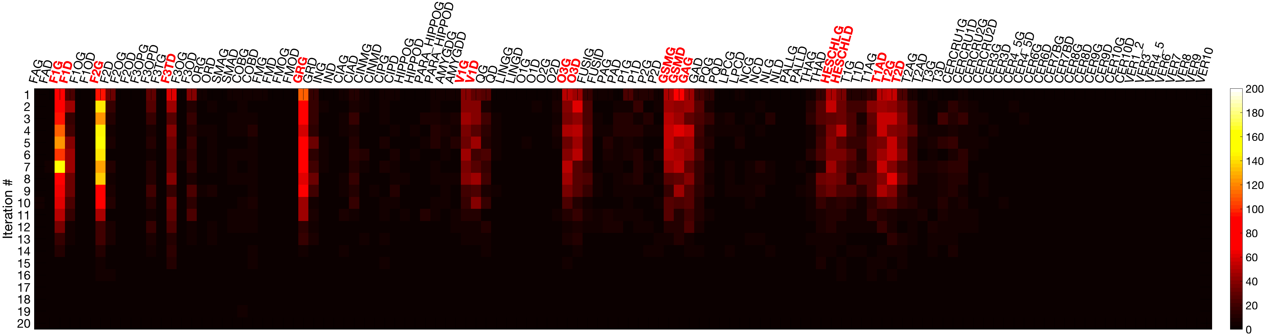
Figure 3: Results of hill climbing variable selection. Results are accumulated over 1000 independently initiated models for left-to-right (A) and right-to-left (B) phase encoding. For each region of interest $\kappa$, the value at the intersection of $\kappa$-th column and $i$-th row represents how often this regions has been selected at the $i$-th iteration of hill climbing. As a result, the dimensionality of the variable space is smaller than the original 116-dimensional variable space, and in most cases it consists of 10 AAL regions. Red colored regions represent the variable space of the most important AAL regions (above $85$-th percentile).

The following areas are identified as the most important AAL regions with respect to the overall contribution to the classification accuracy (Figure 4): Left middle frontal gyrus, lateral part; Left superior frontal gyrus, dorsolateral; Left gyrus rectus; Left middle temporal gyrus; Right supramarginal gyrus; Right superior temporal pole; Left supramarginal gyrus; Right inferior occipital; Left angular gyrus; Left inferior occipital; Right area triangularis; Left transverse temporal gyri; Left calcarine sulcus; Right calcarine sulcus; Right transverse temporal gyri; Right superior frontal gyrus, dorsolateral; Right middle temporal gyrus.

4.2 Comparison Against Logistic Regression

We compared the performance of the proposed pipeline to an often used standard classifier – logistic regression. Given input data $\mathbf{X}=[\mathbf{x}_{1},\dots,\mathbf{x}_{N}]$ and class labels $\mathbf{T}$, linear classifier is a model that maps $\mathbf{X}$ onto $\mathbf{T}$, i.e. $\mathbf{T}=f\big{(}\mathbf{X}^{T}\mathbf{w})$. Here, $\mathbf{w}$ is a vector of model parameters, and $f$ is a function that transforms $\mathbf{X}^{T}\mathbf{w}$ into desired output values. For logistic regression, $f$ is a sigmoid function. In our study, the input data $\mathbf{X}$ is correlation between paired fMRI data, and class labels $\mathbf{T}$ represent zygosity. To train a classifier, we need to find

$$w=\underset{\mathbf{w}}{\operatorname*{arg\,min}}\sum_{i}L(t_{i},y_{i}),$$

where $L(t_{i},y_{i})$ is a log-loss function that measures the discrepancy between the classifier’s prediction value $y_{i}=f(\mathbf{w}^{T}\mathbf{x}_{i})$ and the true class label $t_{i}$ for the $i$-th training example. Logistic regression algorithm finds maximum likelihood estimation of $\mathbf{w}$ using iteratively reweighted least squares (Murphy, 2012):

$$\mathbf{w}^{(k+1)}=\left(\mathbf{X}^{T}\mathbf{S}_{k}\mathbf{X}\right)^{-1}\mathbf{X}^{T}\left(\mathbf{S}_{k}\mathbf{X}\mathbf{w}^{(k)}+\mathbf{T}-\mathbf{Y}^{(k)}\right),$$

where $\mathbf{Y}^{(k)}=[y^{(k)}_{1},\dots,y^{(k)}_{N}]$ is a vector of classifier outputs,

$$y^{(k)}_{i}=\frac{1}{1+e^{-\mathbf{w}^{T}\mathbf{x}_{i}}},\quad\mathbf{S}_{k}=\operatorname{diag}(y^{(k)}_{i}(1-y^{(k)}_{i}))$$

is a diagonal weighting matrix. For the given HCP dataset, we achieved $47.99(\pm 3.32)\%$ classification accuracy with $61.62(\pm 5.56)\%$ false-positive rate and $38.24(\pm 4.14)\%$ false-negative rate employing logistic regression model. Performance wise, the logistic regression was not perform any better than ANN.

Table 4: Most frequent AAL regions selected at the first iteration of hill climbing

Label	Frequency	Accuracy (%)	FPR (%)	FPR (%)
GRG	83/1000	86.36 ($\pm$4.06)	23.04 ($\pm$10.95)	8.68 ($\pm$5.16)
F2G	70/1000	85.03 ($\pm$4.93)	22.43 ($\pm$9.73)	10.66 ($\pm$5.59)
F1G	52/1000	81.63 ($\pm$4.97)	20.74 ($\pm$8.58)	16.92 ($\pm$7.22)
GSMD	50/1000	85.83 ($\pm$6.76)	22.39 ($\pm$10.6)	8.87 ($\pm$6.32)
F3TD	45/1000	86.48 ($\pm$3.82)	18.98 ($\pm$9.36)	9.98 ($\pm$6.39)
T2G	40/1000	86.67 ($\pm$5.44)	19.48 ($\pm$11.79)	10.22 ($\pm$4.97)
T1AD	39/1000	86.09 ($\pm$6.56)	20.43 ($\pm$13.14)	10.61 ($\pm$7.68)
O3G	37/1000	87.69 ($\pm$5.56)	19.5 ($\pm$13.02)	8.46 ($\pm$5.01)
GSMG	36/1000	88.41 ($\pm$4.76)	20.98 ($\pm$12.27)	7.22 ($\pm$4.36)
HESCHLG	36/1000	85.56 ($\pm$7.1)	22.17 ($\pm$13.67)	9.85 ($\pm$5.3)
O3D	34/1000	88.32 ($\pm$4.78)	18.14 ($\pm$11.88)	8.02 ($\pm$5.13)
GAG	34/1000	86.94 ($\pm$4.9)	20.03 ($\pm$8.23)	7.71 ($\pm$6.7)
F3OD	30/1000	85.42 ($\pm$5.24)	20.48 ($\pm$11.06)	11.06 ($\pm$6.19)
V1G	28/1000	87.32 ($\pm$5.11)	22.11 ($\pm$11.69)	5.88 ($\pm$4.75)
HESCHLD	27/1000	84.77 ($\pm$7.22)	21.91 ($\pm$12.99)	11.24 ($\pm$7.92)
F2D	25/1000	86.64 ($\pm$4.3)	20.84 ($\pm$11.6)	9.46 ($\pm$4.23)

FPR: false-positive rate, FNR: false-negative rate. Overall classification accuracy, false-positive rate and false-negative rate are provided with the standard deviation. They present performance of the model at the first iteration of hill climbing when the variable space contains only one variable. Bold font highlights the best performing region. Region names are given in the first column according to the AAL brain atlas specification (http://neuro.compute.dtu.dk/services/brededatabase/index_roi_tzouriomazoyer.html), while the second column displays regions’ labels as they appear on Figure 4. Regions are sorted according to the frequency across 1000 independently initialized models.

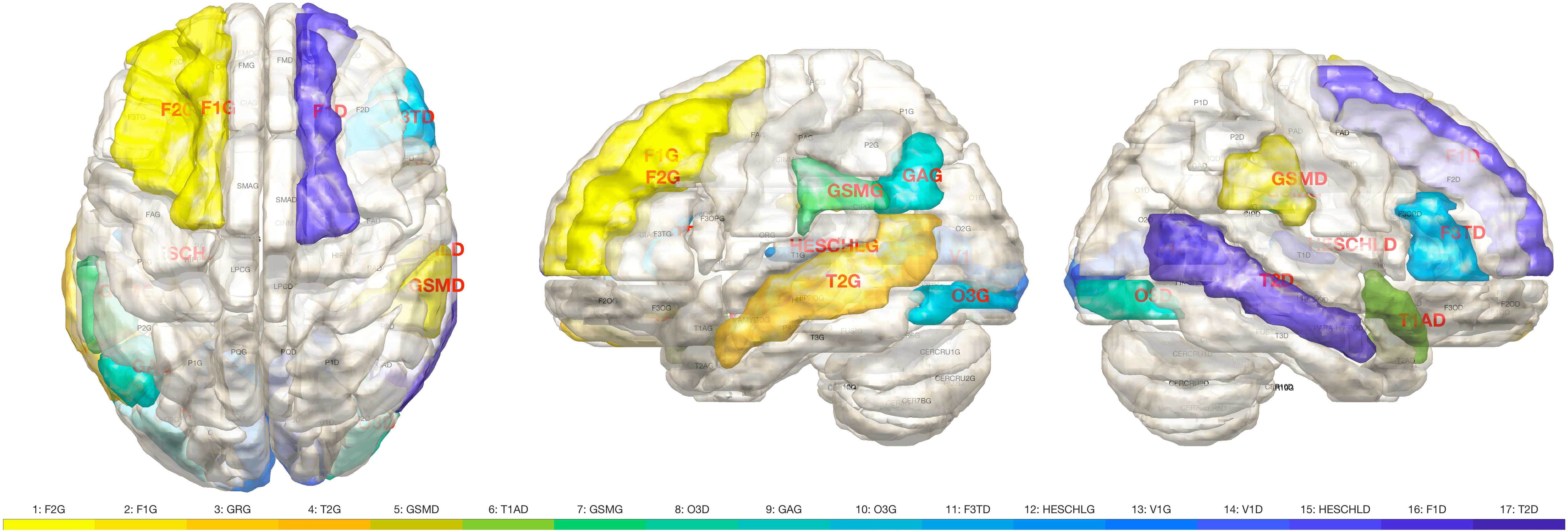
Figure 4: Most heritable brain regions are ranked according to their importance $\mathcal{J}(\kappa)$ and $85$-th percentile regions are colored, which corresponds to regions marked with red font in Figure 3. Refer to Table 4 for a detailed information on the contribution of each parcellation to the performance of classification model.

5 Conclusion and Discussion

For the first time, we addressed the problem of classifying the zygosity of twin-pairs using resting state functional MRI. This is a more complex problem than the usual classification problem of labeling each image into distinct classes. Here, we are interested in learning if the relationship between pairs of images is associated with the zygosity of twins.

There are two practical advantages for using CSR as a new feature representation of twin fMRI. First, employing cosine series representation allows to correlate fMRI signals in the frequency domain. Furthermore, representing the original fMRI signals as a linear combination of 120 cosine basis functions serves not only as a dimensionality reduction technique but also as a means of denoising high frequency noise. To emphasize the importance of the new feature representation in the performance of classification, we classified twin fMRI without the cosine series representation (CSR) and obtained $54.15(\pm 9.24)\%$ classification accuracy (Table 3, first row). The use of CSR allowed us to increase the classification accuracy to $79.93(\pm 7.59)\%$, which is an increase of $25\%$. The proposed framework of ANN with hill climbing achieves the classification accuracy of $94.19(\pm 3.53)\%$ in identifying the zygosity of twins. Performance of the proposed classification pipeline is much higher when compared to the accuracy achieved on the same dataset by a conventional classification model - logistic regression, $47.99(\pm 3.32)\%$.

Regions with significant genetic influence

We report that the most genetically affected brain regions, as measured by their contribution to the classification accuracy of the zygosity type of twins, are mainly located in the temporo-parietal and frontal brain regions. In order to determine if our findings are consistent with previous studies, we examined previous twin imaging studies. Despite some discrepancy, there is a overlap of our findings with results reported in a number of twin studies of both task-based and resting-state functional MRI (Blokland et al., 2008, 2011; Koten et al., 2009; Glahn et al., 2010; Park et al., 2012; Gao et al., 2014; Sinclair et al., 2015; Yang et al., 2016). Cannon et al. (2002) found that genetic influences were isolated primarily to polar, inferior, and dorsolateral prefrontal brain areas, and also in the frontal regions. Matthews et al. (2007) found that dorsal anterior cingulate cortex activation is significantly influenced by genes. Pietiläinen et al. (2008) demonstrated high heritability of medial and dorsolateral prefrontal cortex. Blokland et al. (2008, 2011) found that the inferior, middle, and superior frontal gyri, left supplementary motor area, precentral and postcentral gyri, middle cingulate cortex, superior medial gyrus, angular gyrus, superior parietal lobule, including precuneus, and superior occipital gyri are genetically affected in twins. Koten et al. (2009) observed significant genetic influences on brain activation in visual cortex, temporo-parietal and frontal areas, and anterior cingulate cortex. Park et al. (2012) found neural activity in the left visual cortex and left motor cortex were significantly heritable. Sinclair et al. (2015) found that 47 out of 116 AAL regions are significantly heritable which overlap with most of our regions. Compared to previous twin literature, there is a strong consistency in the identifeid heritable brain regions. However disparities suggest that genetic influences may vary with task paradigms, which rs-fMRI is lacking.

AAL parcellation template

In the proposed framework, we computed pairwise correlation between twin subjects and then averaged them using the predefined AAL parcellation. However, from the review of several structural and functional voxel-based twin studies, it is apparent that genetic effects may carry across anatomical boundaries (Blokland et al., 2011; Joshi et al., 2011; van Soelen et al., 2012). Therefore, voxel-based approaches may have preference in imaging genetic studies over ROI approaches that average measurements across brain parcels. The drawback of voxel-wise approaches in general is an extensive computational load resulting from the computation of pairwise correlations at voxel level. We overcame this drawback by utilizing 120-degree cosine series representation that drastically decreases computational time by compact signal representation. We take the advantage of both methods in increasing the classification accuracy. Although we demonstrated relatively high classification accuracy with a provided solution, there is a need for better parcellation method that balances the trade-off between pure voxel-wise and anatomical template-based approaches. We leave this as a future study.

Variable selection

To quantify the extent of genetic contribution of AAL parcellations, we used hill climbing – a greedy search algorithm that considers regions of interest as independent variables and tests one variable at a time. Recent studies of both resting-state and task-related fMRI on the functional connectivity of brain regions has revealed that activity in some regions may have strong coherence (Jansen et al., 2015; Yang et al., 2016). To get a more accurate inference on the optimal variable space, one may consider applying the concept of ”connectivity of regions” and performing a group variable selection, i.e., combine variables in groups and test each group as a single instance (Russell & Norvig, 2003). Additionally, this will reduce computational load of variable selection procedure, whose computational complexity for brute-force approaches that test all possible combinations of variables is $\mathcal{O}(2^{n})$ (Yang et al., 2016). Other type of more complex variable selection methods are left as a future study.

References

- (1)
- Babajani-Feremi (2017) Babajani-Feremi, A. (2017), ‘Neural Mechanism Underling Comprehension of Narrative Speech and Its Heritability: Study in a Large Population’, Brain Topography 30(5), 592–609.
- Biswal et al. (1997) Biswal, B. B., van Kylen, J. & Hyde, J. S. (1997), ‘Simultaneous Assessment of Flow and BOLD Signals in Resting‐state Functional Connectivity Maps’, NMR in Biomedicine 10(4‐5), 165–170.
- Blokland et al. (2011) Blokland, G. A. M., McMahon, K. L., Thompson, P. M., Martin, N. G., de Zubicaray, G. I. & Wright, M. J. (2011), ‘Heritability of Working Memory Brain Activation’, Journal of Neuroscience 31(30), 10882–10890.
- Blokland et al. (2008) Blokland, G. A., McMahon, K. L., Hoffman, J., Zhu, G., Meredith, M., Martin, N. G., Thompson, P. M., de Zubicaray, G. I. & Wright, M. J. (2008), ‘Quantifying the Heritability of Task-related Brain Activation and Performance During the N-back Working Memory Task: A twin fMRI study’, Biological Psychology 79(1), 70 – 79.
- Bromley et al. (1994) Bromley, J., Guyon, I., LeCun, Y., Säckinger, E. & Shah, R. (1994), Signature Verification Using a ”Siamese” Time Delay Neural Network, in ‘Advances in Neural Information Processing Systems’, pp. 737–744.
- Cannon et al. (2002) Cannon, T. D., Thompson, P. M., van Erp, T. G. M., Toga, A. W., Poutanen, V.-P., Huttunen, M., Lonnqvist, J., Standerskjold-Nordenstam, C.-G., Narr, K. L., Khaledy, M., Zoumalan, C. I., Dail, R. & Kaprio, J. (2002), ‘Cortex Mapping Reveals Regionally Specific Patterns of Genetic and Disease-specific Gray-matter Deficits in Twins Discordant for Schizophrenia’, Proceedings of the National Academy of Sciences 99(5), 3228–3233.
- Curtis et al. (2005) Curtis, C., Sun, F., Miller, L. & D’esposito, M. (2005), ‘Coherence between fMRI time-series distinguishes two spatial working memory networks’, Neuroimage 26, 177–183.
- Falconer et al. (1996) Falconer, D. S., Mackay, T. F. & Frankham, R. (1996), Introduction to Quantitative Genetics (4th edn), Pearson Education.
- Finn et al. (2015) Finn, E., Shen, X., Scheinost, D., Rosenberg, M., Jessica, H., M Chun, M., Papademetris, X. & Constable, R. (2015), ‘Functional connectome fingerprinting: Identifying individuals using patterns of brain connectivity’, Nature Neuroscience 18, 1664.
- Fornito et al. (2011) Fornito, A., Zalesky, A., Bassett, D. S., Meunier, D., Ellison-Wright, I., Yücel, M., Wood, S. J., Shaw, K., O’Connor, J., Nertney, D., Mowry, B. J., Pantelis, C. & Bullmore, E. T. (2011), ‘Genetic Influences on Cost-Efficient Organization of Human Cortical Functional Networks’, Journal of Neuroscience 31(9), 3261–3270.
- Gao et al. (2014) Gao, W., Elton, A., Zhu, H., Alcauter, S., Smith, J. K., Gilmore, J. H. & Lin, W. (2014), ‘Intersubject Variability of and Genetic Effects on the Brain’s Functional Connectivity during Infancy’, Journal of Neuroscience 34(34), 11288–11296.
- Glahn et al. (2010) Glahn, D. C., Winkler, A. M., Kochunov, P., Almasy, L., Duggirala, R., Carless, M. A., Curran, J. C., Olvera, R. L., Laird, A. R., Smith, S. M., Beckmann, C. F., Fox, P. T. & Blangero, J. (2010), ‘Genetic Control over the Resting Brain’, Proceedings of the National Academy of Sciences 107(3), 1223–1228.
- Glasser et al. (2013) Glasser, M. F., Sotiropoulos, S. N., Wilson, J. A., Coalson, T. S., Fischl, B., Andersson, J. L., Xu, J., Jbabdi, S., Webster, M., Polimeni, J. R., Essen, D. C. V. & Jenkinson, M. (2013), ‘The Minimal Preprocessing Pipelines for the Human Connectome Project’, NeuroImage 80, 105 – 124.
- Guo et al. (2017) Guo, Y., Gao, Y. & Shen, D. (2017), Chapter 9 - deformable mr prostate segmentation via deep feature learning and sparse patch matching, in S. K. Zhou, H. Greenspan & D. Shen, eds, ‘Deep Learning for Medical Image Analysis’, Academic Press, pp. 197 – 222.
- Hagan et al. (2014) Hagan, M. T., Demuth, H. B., Beale, M. H. & De Jess, O. (2014), Neural Network Design, 2nd edn, Martin Hagan, USA.
- Honorio (2015) Honorio, J. (2015), Classification on Brain Functional Magnetic Resonance Imaging: Dimensionality, Sample Size, Subject Variability and Noise, in ‘Frontiers of Medical Imaging’, World Scientific, pp. 153–165.
- Jansen et al. (2015) Jansen, A. G., Mous, S. E., White, T., Posthuma, D. & Polderman, T. J. (2015), ‘What Twin Studies Tell Us About the Heritability of Brain Development, Morphology, and Function: a Review’, Neuropsychology Review 25(1), 27–46.
- Joshi et al. (2017) Joshi, A. A., Chong, M. & Leahy, R. M. (2017), Brainsync: An orthogonal transformation for synchronization of fmri data across subjects, in M. Descoteaux, L. Maier-Hein, A. Franz, P. Jannin, D. L. Collins & S. Duchesne, eds, ‘Medical Image Computing and Computer Assisted Intervention - MICCAI 2017’, Springer International Publishing, Cham, pp. 486–494.
- Joshi et al. (2011) Joshi, A. A., Lepore, N., Joshi, S. H., Lee, A. D., Barysheva, M., Stein, J. L., McMahon, K. L., Johnson, K., de Zubicaray, G. I., Martin, N. G. et al. (2011), ‘The Contribution of Genes to Cortical Thickness and Volume’, Neuroreport 22(3), 101–105.
- Karlsgodt et al. (2007) Karlsgodt, K. H., Glahn, D. C., van Erp, T. G., Therman, S., Huttunen, M., Manninen, M., Kaprio, J., Cohen, M. S., Lönnqvist, J. & Cannon, T. D. (2007), ‘The Relationship Between Performance and fMRI Signal During Working Memory in Patients with Schizophrenia, Unaffected Co-twins, and Control Subjects’, Schizophrenia Research 89(1), 191 – 197.
- Koten et al. (2009) Koten, J. W., Wood, G., Hagoort, P., Goebel, R., Propping, P., Willmes, K. & Boomsma, D. I. (2009), ‘Genetic Contribution to Variation in Cognitive Function: An fMRI Study in Twins’, Science 323(5922), 1737–1740.
- Kouw et al. (2017) Kouw, W. M., Loog, M., Bartels, L. W. & Mendrik, A. M. (2017), ‘MR Acquisition-Invariant Representation Learning’, arXiv preprint arXiv:1709.07944 .
- Ktena et al. (2017) Ktena, S. I., Parisot, S., Ferrante, E., Rajchl, M., Lee, M., Glocker, B. & Rueckert, D. (2017), Distance Metric Learning Using Graph Convolutional Networks: Application to Functional Brain Networks, in M. Descoteaux, L. Maier-Hein, A. Franz, P. Jannin, D. L. Collins & S. Duchesne, eds, ‘Medical Image Computing and Computer Assisted Intervention – MICCAI 2017’, Springer International Publishing, Cham, pp. 469–477.
- Ktena et al. (2018) Ktena, S. I., Parisot, S., Ferrante, E., Rajchl, M., Lee, M., Glocker, B. & Rueckert, D. (2018), ‘Metric Learning with Spectral Graph Convolutions on Brain Connectivity Networks’, NeuroImage 169, 431 – 442.
-
LaConte et al. (2005)
LaConte, S., Strother, S., Cherkassky, V., Anderson, J. & Hu, X.
(2005), ‘Support vector machines for
temporal classification of block design fmri data’, NeuroImage 26(2), 317 – 329.
http://www.sciencedirect.com/science/article/pii/S1053811905000893 -
Liang et al. (2012)
Liang, X., Wang, J., Yan, C., Shu, N., Xu, K., Gong, G. & He, Y.
(2012), ‘Effects of different correlation
metrics and preprocessing factors on small-world brain functional networks: A
resting-state functional mri study’, PLOS ONE 7(3), 1–16.
https://doi.org/10.1371/journal.pone.0032766 - Liu et al. (2018) Liu, J., Pan, Y., Li, M., Chen, Z., Tang, L., Lu, C. & Wang, J. (2018), ‘Applications of deep learning to mri images: A survey’, Big Data Mining and Analytics 1(1), 1–18.
- Maes (2005) Maes, H. H. (2005), ACE Model, in ‘Encyclopedia of Statistics in Behavioral Science’, John Wiley & Sons, Ltd.
- Matthews et al. (2007) Matthews, S. C., Simmons, A. N., Strigo, I., Jang, K., Stein, M. B. & Paulus, M. P. (2007), ‘Heritability of Anterior Cingulate Response to Conflict: An fMRI Study in Female Twins’, NeuroImage 38(1), 223 – 227.
- Minnesota Center for Twin and Family Research (2007) Minnesota Center for Twin and Family Research (2007), ‘Minnesota twin family study: Twin info and frequently asked questions’, https://mctfr.psych.umn.edu/twinstudy/twin%20FAQ.html. Accessed: 2018-09-05.
- Miranda-Dominguez et al. (2014) Miranda-Dominguez, O., Mills, B. D., Carpenter, S. D., Grant, K. A., Kroenke, C. D., Nigg, J. T. & Fair, D. A. (2014), ‘Connectotyping: model based fingerprinting of the functional connectome’, PloS one 9(11), e111048.
- Møller (1993) Møller, M. F. (1993), ‘A Scaled Conjugate Gradient Algorithm for Fast Supervised Learning’, Neural Networks 6(4), 525–533.
- Murphy (2012) Murphy, K. P. (2012), Machine learning: a probabilistic perspective, The MIT Press, Cambridge, MA.
- Neale & Cardon (2013) Neale, M. C. & Cardon, L. R. (2013), Methodology for Genetic Studies of Twins and Families, Vol. 67, Springer Science & Business Media.
- Ombao & Van Bellegem (2008) Ombao, H. & Van Bellegem, S. (2008), ‘Evolutionary coherence of nonstationary signals’, IEEE Transactions on Signal Processing 56, 2259–2266.
- Park et al. (2012) Park, J., Shedden, K. & Polk, T. A. (2012), ‘Correlation and Heritability in Neuroimaging Datasets: A Spatial Decomposition Approach with Application to an fMRI Study of Twins’, NeuroImage 59(2), 1132 – 1142.
-
Peltier et al. (2005)
Peltier, S. J., LaConte, S. M., Niyazov, D. M., Liu, J. Z., Sahgal, V., Yue,
G. H. & Hu, X. P. (2005),
‘Reductions in interhemispheric motor cortex functional connectivity after
muscle fatigue’, Brain Research 1057(1), 10 – 16.
http://www.sciencedirect.com/science/article/pii/S0006899305009625 - Peltier et al. (2009) Peltier, S. J., Lisinski, J. M., Noll, D. C. & LaConte, S. M. (2009), Support Vector Machine Classification of Complex fMRI Data, in ‘2009 Annual International Conference of the IEEE Engineering in Medicine and Biology Society’, pp. 5381–5384.
- Pereira et al. (2009) Pereira, F., Mitchell, T. & Botvinick, M. (2009), ‘Machine Learning Classifiers and fMRI: A Tutorial Overview’, NeuroImage 45(1, Supplement 1), S199 – S209.
- Pietiläinen et al. (2008) Pietiläinen, O. P., Paunio, T., Loukola, A., Tuulio‐Henriksson, A., Kieseppä, T., Thompson, P., Toga, A. W., van Erp, T. G., Silventoinen, K., Soronen, P., Hennah, W., Turunen, J. A., Wedenoja, J., Palo, O. M., Silander, K., Lönnqvist, J., Kaprio, J., Cannon, T. D. & Peltonen, L. (2008), ‘Association of AKT1 with Verbal Learning, Verbal Memory, and Regional Cortical Gray Matter Density in Twins’, American Journal of Medical Genetics Part B: Neuropsychiatric Genetics 150B(5), 683–692.
- Pinel & Dehaene (2013) Pinel, P. & Dehaene, S. (2013), ‘Genetic and Environmental Contributions to Brain Activation During Calculation’, NeuroImage 81, 306 – 316.
- Richmond et al. (2016) Richmond, S., Johnson, K. A., Seal, M. L., Allen, N. B. & Whittle, S. (2016), ‘Development of Brain Networks and Relevance of Environmental and Genetic Factors: A Systematic Review’, Neuroscience & Biobehavioral Reviews 71, 215 – 239.
-
Rogers et al. (2007)
Rogers, B. P., Morgan, V. L., Newton, A. T. & Gore, J. C.
(2007), ‘Assessing functional connectivity
in the human brain by fmri’, Magnetic Resonance Imaging 25(10), 1347 – 1357.
http://www.sciencedirect.com/science/article/pii/S0730725X07002238 - Russell & Norvig (2003) Russell, S. J. & Norvig, P. (2003), Artificial Intelligence: A Modern Approach, 2 edn, Pearson Education.
- Sanroma et al. (2018) Sanroma, G., Benkarim, O. M., Piella, G., Camara, O., Wu, G., Shen, D., Gispert, J. D., Molinuevo, J. L. & Ballester, M. A. G. (2018), ‘Learning non-linear patch embeddings with neural networks for label fusion’, Medical Image Analysis 44, 143 – 155.
- Sinclair et al. (2015) Sinclair, B., Hansell, N. K., Blokland, G. A., Martin, N. G., Thompson, P. M., Breakspear, M., de Zubicaray, G. I., Wright, M. J. & McMahon, K. L. (2015), ‘Heritability of the Network Architecture of Intrinsic Brain Functional Connectivity’, NeuroImage 121, 243 – 252.
- Singh et al. (2007) Singh, V., Miyapuram, K. P. & Bapi, R. S. (2007), Detection of Cognitive States from fMRI Data Using Machine Learning Techniques, in ‘2007 International Joint Conference on Artificial Intelligence (IJCAI)’, pp. 587–592.
- Smith et al. (2013) Smith, S. M., Beckmann, C. F., Andersson, J., Auerbach, E. J., Bijsterbosch, J., Douaud, G., Duff, E., Feinberg, D. A., Griffanti, L., Harms, M. P., Kelly, M., Laumann, T., Miller, K. L., Moeller, S., Petersen, S., Power, J., Salimi-Khorshidi, G., Snyder, A. Z., Vu, A. T., Woolrich, M. W., Xu, J., Yacoub, E., Uğurbil, K., Essen, D. C. V. & Glasser, M. F. (2013), ‘Resting-state fMRI in the Human Connectome Project’, NeuroImage 80, 144 – 168.
- Smith et al. (2015) Smith, S. M., Nichols, T. E., Vidaurre, D., Winkler, A. M., Behrens, T. E., Glasser, M. F., Ugurbil, K., Barch, D. M., Van Essen, D. C. & Miller, K. L. (2015), ‘A positive-negative mode of population covariation links brain connectivity, demographics and behavior’, Nature neuroscience 18(11), 1565.
- van den Heuvel et al. (2013) van den Heuvel, M. P., van Soelen, I. L., Stam, C. J., Kahn, R. S., Boomsma, D. I. & Pol, H. E. H. (2013), ‘Genetic Control of Functional Brain Network Efficiency in Children’, European Neuropsychopharmacology 23(1), 19 – 23.
- Van Essen et al. (2013) Van Essen, D. C., Smith, S. M., Barch, D. M., Behrens, T. E., Yacoub, E. & Ugurbil, K. (2013), ‘The WU-Minn Human Connectome Project: An Overview’, NeuroImage 80, 62 – 79.
- Van Essen & Ugurbil (2012) Van Essen, D. C. & Ugurbil, K. (2012), ‘The Future of the Human Connectome’, NeuroImage 62(2), 1299 – 1310.
- Van Essen et al. (2012) Van Essen, D. C., Ugurbil, K., Auerbach, E., Barch, D., Behrens, T., Bucholz, R., Chang, A., Chen, L., Corbetta, M., Curtiss, S. W., Penna, S. D., Feinberg, D., Glasser, M. F., Harel, N., Heath, A., Larson-Prior, L., Marcus, D., Michalareas, G., Moeller, S., Oostenveld, R., Petersen, S. E., Prior, F., Schlaggar, B. L., Smith, S. M., Snyder, A. Z., Xu, J. & Yacoub, E. (2012), ‘The Human Connectome Project: A Data Acquisition Perspective’, NeuroImage 62(4), 2222–2231.
- van Soelen et al. (2012) van Soelen, I., Brouwer, R., van Baal, G., Schnack, H., Peper, J., Collins, D., Evans, A., Kahn, R., Boomsma, D. & Pol, H. H. (2012), ‘Genetic influences on thinning of the cerebral cortex during development’, NeuroImage 59(4), 3871 – 3880.
- Vergun et al. (2013) Vergun, S., Deshpande, A., Meier, T., Song, J., Tudorascu, D., Nair, V., Singh, V., Biswal, B., Meyerand, M., Birn, R. & Prabhakaran, V. (2013), ‘Characterizing Functional Connectivity Differences in Aging Adults using Machine Learning on Resting State fMRI Data’, Frontiers in Computational Neuroscience 7, 38.
- Vrbik (2005) Vrbik, J. (2005), ‘Population Moments of Sampling Distributions’, Computational Statistics 20(4), 611–621.
- Wang & Yang (2018) Wang, J. & Yang, Y. (2018), ‘A Context-sensitive Deep Learning Approach for Microcalcification Detection in Mammograms’, Pattern Recognition 78, 12 – 22.
- Wang et al. (2014) Wang, J., You, X., Wu, W., Guillen, M. R., Cabrerizo, M., Sullivan, J., Donner, E., Bjornson, B., Gaillard, W. D. & Adjouadi, M. (2014), ‘Classification of fMRI Patterns—A Study of the Language Network Segregation in Pediatric Localization Related Epilepsy’, Human Brain Mapping 35(4), 1446–1460.
- Wang et al. (2015) Wang, Q., Kim, M., Shi, Y., Wu, G. & Shen, D. (2015), ‘Predict brain mr image registration via sparse learning of appearance and transformation’, Medical Image Analysis 20(1), 61 – 75.
- Wang et al. (2017) Wang, X., Ren, Y. & Zhang, W. (2017), ‘Depression Disorder Classification of fMRI Data Using Sparse Low-Rank Functional Brain Network and Graph-Based Features’, Computational and Mathematical Methods in Medicine 2017.
- WU-Minn HCP Consortium (2018) WU-Minn HCP Consortium (2018), ‘1200 Subjects Data Release’, Reference Manual .
- Yang et al. (2016) Yang, Z., Zuo, X.-N., McMahon, K. L., Craddock, R. C., Kelly, C., de Zubicaray, G. I., Hickie, I., Bandettini, P. A., Castellanos, F. X., Milham, M. P. & Wright, M. J. (2016), ‘Genetic and Environmental Contributions to Functional Connectivity Architecture of the Human Brain’, Cerebral Cortex 26(5), 2341–2352.
- Zagoruyko & Komodakis (2015) Zagoruyko, S. & Komodakis, N. (2015), Learning to Compare Image Patches via Convolutional Neural Networks, in ‘Computer Vision and Pattern Recognition (CVPR), 2015 IEEE Conference on’, IEEE, pp. 4353–4361.