Model-independent sensibility studies for the anomalous dipole moments of the $\nu_{\tau}$ at the CLIC based $\gamma e^{-}$ colliders

Abstract

To improve the theoretical prediction of the anomalous dipole moments of the $\tau$-neutrino, we have carried out a study through the process $\gamma e^{-}\to\tau\bar{\nu}_{\tau}\nu_{e}$, which represents an excellent and useful option in determination of these anomalous parameters. To study the potential of the process $\gamma e^{-}\to\tau\bar{\nu}_{\tau}\nu_{e}$, we apply a future high-energy and high-luminosity linear electron-positron collider, such as the CLIC, with $\sqrt{s}=380,1500,3000\hskip 2.27621ptGeV$ and ${\cal L}=10,50,100,200,500,1000,1500,2000,3000\hskip 2.27621ptfb^{-1}$, and we consider systematic uncertainties of $\delta_{sys}=0,5,10\%$. With these elements, we present a comprehensive and detailed sensitivity study on the total cross-section of the process $\gamma e^{-}\to\tau\bar{\nu}_{\tau}\nu_{e}$, as well as on the dipole moments $\mu_{\nu_{\tau}}$ and $d_{\nu_{\tau}}$ at the $95\%$ C.L., showing the feasibility of such process at the CLIC at the $\gamma e^{-}$ mode with unpolarized and polarized electron beams.

I Introduction

The magnetic and electric dipole moments of the neutrino ($\nu$MM) and ($\nu$EDM) are one of the most sensitive probes of physics beyond the Standard Model (BSM). On this topic, in the original formulation of the Standard Model (SM) Glashow ; Weinberg ; Salam neutrinos are massless particles with zero $\nu$MM. However, in the minimally extended SM containing gauge-singlet right-handed neutrinos, the $\nu$MM induced by radiative corrections is unobservably small, $\mu_{\nu}=3eG_{F}m_{\nu_{i}}/(8\sqrt{2}\pi^{2})\simeq 3.1\times 10^{-19}(m_{\nu_{i}}/1\hskip 2.84526pteV)\mu_{B}$, where $\mu_{B}=e/2m_{e}$ is the Bohr magneton Fujikawa ; Shrock . Present experimental limits on these $\nu$MM are several orders of magnitude larger, so that a MM close to these limits would indicate a window for probing effects induced by new physics BSM Fukugita . Similarly, a $\nu$EDM will also point to new physics and will be of relevance in astrophysics and cosmology, as well as terrestrial neutrino experiments Cisneros .

A fundamental challenge of the particle physics community is to determine the Majorana or Dirac nature of the neutrino. For respond to this challenge, experimentalist are exploring different reactions where the Majorana nature may manifest Zralek . About this topic, the study of neutrino magnetic moments is, in principle, a way to distinguish between Dirac and Majorana neutrinos since the Majorana neutrinos can only have flavor changing, transition magnetic moments while the Dirac neutrinos can only have flavor conserving one.

Another fundamental challenge posed by the scientific community is the following: are the laws of physics the same for matter and anti-matter, or are matter and anti-matter intrinsically different ? It is possible that the answer to this problem may hold the key to solving the mystery of the matter-dominated Universe ? A. Sakharov proposed a solution to this problem Sakharov , your proposal requires the violation of a fundamental symmetry of nature: the CP symmetry. The study of CP violation addresses this problem, as well as many other predicted for the SM. The SM predict CP violation, which is necessary for the existence of the electric dipole moments (EDM) of a variety physical systems. The EDM provides a direct experimental probe of CP violation Christenson ; Abe ; Aaij , a feature of the SM and beyond SM physics. The signs of new physics can be analyzed by investigating the electromagnetic dipole moments of the tau-neutrino, such as its MM and EDM. In recent years, the $\nu_{\tau}$EDM have received much attention because the experimental sensitivity is expected to improve considerably in the future. Precise measurement of the $\nu_{\tau}$EDM is an important probe of CP violation.

In the case of the $\nu_{e}$MM and $\nu_{\mu}$MM, the best current sensitivity limits are derived from reactor neutrino experiment GEMMA Bed and of the Liquid Scintillator Neutrino Detector (LSND) experiment Auerbach , respectively. The obtained sensitivity limits are

$$\mu^{exp}_{\nu_{e}}=2.9\times 10^{-11}\mu_{B},\hskip 8.53581pt90\%\hskip 5.69054ptC.L.\hskip 14.22636pt\mbox{[GEMMA]}\hskip 14.22636pt\mbox{\cite[cite]{\@@bibref{Authors Phrase1YearPhrase2}{Bed}{\@@citephrase{(}}{\@@citephrase{)}}}},$$ (1)

$$\mu^{exp}_{\nu_{\mu}}=6.8\times 10^{-10}\mu_{B},\hskip 8.53581pt90\%\hskip 5.69054ptC.L.\hskip 14.22636pt\mbox{[LSND]}\hskip 14.22636pt\mbox{\cite[cite]{\@@bibref{Authors Phrase1YearPhrase2}{Auerbach}{\@@citephrase{(}}{\@@citephrase{)}}}},$$ (2)

these limits are eight-nine orders of magnitude weaker than the SM prediction.

For the electric dipole moments $d_{\nu_{e},\nu_{\mu}}$ Aguila the best bounds are:

$$d_{\nu_{e},{\nu}_{\mu}}<2\times 10^{-21}(ecm),\hskip 14.22636pt95\%\hskip 2.27621ptC.L..\\$$ (3)

For the tau-neutrino, the bounds on their dipole moments are less restrictive, and therefore it is worth investigating in deeper way their electromagnetic properties. The $\tau$-neutrino correspond to the more massive third generation of leptons and possibly possesses the largest mass and the largest magnetic and electric dipole moments.

Table I of Ref. Gutierrez10 , summary the current experimental and theoretical bounds on the anomalous dipole moments of the tau-neutrino. The present experimental bounds on the anomalous magnetic moment of the tau-neutrino has been reported by different experiments at Borexino Borexino , E872 (DONUT) DONUT , CERN-WA-066 A.M.Cooper , and at LEP L3 . In addition, other limits on the $\nu_{\tau}$MM and $\nu_{\tau}$EDM in different context are reported in Refs. Gutierrez12 ; Gutierrez11 ; Gutierrez10 ; Gutierrez9 ; Gutierrez8 ; Data2016 ; Gutierrez7 ; Gutierrez6 ; Aydin ; Gutierrez5 ; Gutierrez4 ; Gutierrez3 ; Keiichi ; Aytekin ; Gutierrez2 ; Gutierrez1 ; DELPHI ; Escribano ; Gould ; Grotch ; Sahin ; Sahin1 .

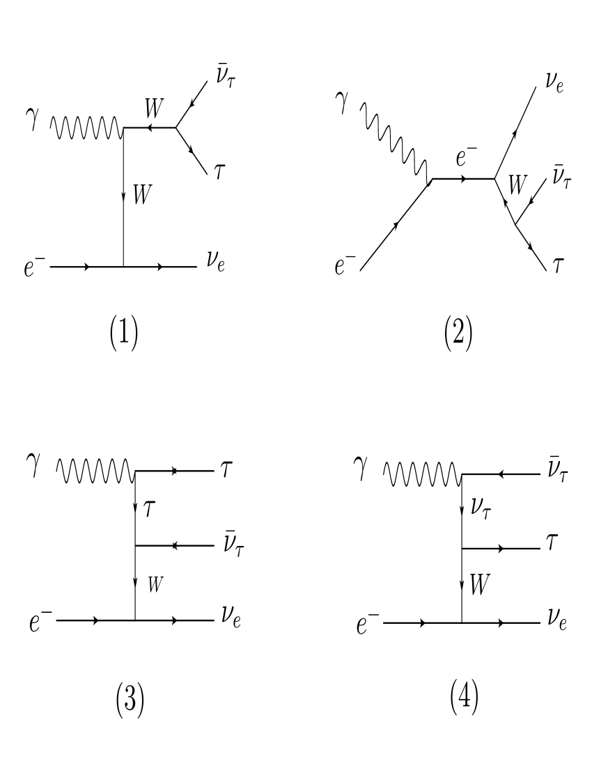
Figure 1: The Feynman diagrams contributing to the process $\gamma e^{-}\to\tau\bar{\nu}_{\tau}\nu_{e}$.

For the study of the dipole moments of the $\nu_{\tau}$ we consider the process $\gamma e^{-}\to\tau\bar{\nu}_{\tau}\nu_{e}$, in the presence of anomalous magnetic and electric dipole couplings $\mu_{\nu_{\tau}}$ and $d_{\nu_{\tau}}$, respectively. The set Feynman diagrams are given in Fig. 1. The final state given by $\gamma e^{-}\to\tau\bar{\nu}_{\tau}\nu_{e}$ is considered with the subsequent decay of the tau-lepton through two different decay channels, the leptonic decay channel and the hadronic decay channel.

The neutrino is a neutral particle, therefore its electromagnetic properties appear only at loop level. However, a method of studying these properties on a model-independent form is to consider the effective neutrino-photon interaction. In this regard, the most general expression consistent with Lorentz and electromagnetic gauge invariance, for the tau-neutrino electromagnetic vertex may be parameterized in terms of four form factors Nieves ; Kayser ; Kayser1 :

$$\Gamma^{\alpha}=eF_{1}(q^{2})\gamma^{\alpha}+\frac{ie}{2m_{\nu_{\tau}}}F_{2}(q^{2})\sigma^{\alpha\mu}q_{\mu}+\frac{e}{2m_{\nu_{\tau}}}F_{3}(q^{2})\gamma_{5}\sigma^{\alpha\mu}q_{\mu}+eF_{4}(q^{2})\gamma_{5}(\gamma^{\alpha}-\frac{q\hbox to0.0pt{\hss/}q^{\alpha}}{q^{2}}),$$ (4)

where $e$ is the charge of the electron, $m_{\nu_{\tau}}$ is the mass of the tau-neutrino, $q^{\mu}$ is the photon momentum, and $F_{1,2,3,4}(q^{2})$ are the electromagnetic form factors of the neutrino, corresponding to charge radius, MM, EDM and anapole moment (AM), respectively, at $q^{2}=0$ Escribano ; Vogel ; Bernabeu1 ; Bernabeu2 ; Dvornikov ; Giunti ; Broggini .

The future $e^{+}e^{-}$ linear colliders are being designed to function also as $\gamma\gamma$ or $\gamma e^{-}$ colliders with the photon beams generated by laser-backscattering method, in these modes the flexibility in polarizing both lepton and photon beams will allow unique opportunities to analyze the tau-neutrino properties and interactions. It is therefore conceivable to exploit the sensitivity of these $\gamma e^{-}$ colliders based on $e^{+}e^{-}$ linear colliders of center-of-mass energies of $380-3000\hskip 2.27621ptGeV$. See Refs. Ginzburg ; Telnov ; Milburn ; Arutyunyan for a detailed description of the $\gamma\gamma$ and $\gamma e^{-}$ colliders.

To study the sensitivity on the anomalous dipole moments of the tau-neutrino, we consider a future high-energy and high-luminosity linear electron positron collider, such as the Compact Linear Collider (CLIC) Accomando ; Dannheim ; Abramowicz , with center-of-mass energies of $\sqrt{s}=380,1500,3000\hskip 2.27621ptGeV$ and luminosities of ${\cal L}=10,50,100,200,500,1000,1500,2000,3000\hskip 2.27621ptfb^{-1}$. Furthermore, we apply systematic uncertainties of $\delta_{sys}=0,5,10\%$, as well as polarized electron beams which affect the total and angular cross-section.

This article is organized as follows. In Section II, we study the total cross-section and the dipole moments of the tau-neutrino through the process $\gamma e^{-}\to\tau\bar{\nu}_{\tau}\nu_{e}$ with unpolarized and polarized beams. The Section III is devoted to our conclusions.

II Cross-section of the process $\gamma e^{-}\to\tau\bar{\nu}_{\tau}\nu_{e}$ with unpolarized and polarized beams

The CLIC physics program Accomando ; Dannheim ; Abramowicz is very broad and rich which complements the physics program of the LHC. Furthermore, it provides a unique opportunity to study $\gamma\gamma$ and $\gamma e^{-}$ interactions with energies and luminosities similar to those in $e^{+}e^{-}$ collisions.

On the other hand, although many particles and processes can be produced in both colliders $e^{+}e^{-}$ and $\gamma\gamma$, $\gamma e^{-}$ the reactions are different and will give complementary and very valuable information about new physics phenomena, such as is the case of the dipole moments of the tau-neutrino which we study through the process $\gamma e^{-}\to\tau\bar{\nu}_{\tau}\nu_{e}$. Fig. 1 shows the Feynman diagrams corresponding to said process. Our numerical analyses are carried out using the CALCHEP 3.6.30 Calhep package, which can computate the Feynman diagrams, integrate over multiparticle phase space and event simulation.

We evaluate the total cross-section of the process $\gamma e^{-}\to\tau\bar{\nu}_{\tau}\nu_{e}$ as a function of the anomalous form factors $F_{2}$, $F_{3}$ and $(F_{2},F_{3})$ and tau lepton decays hadronic and leptonic modes are considered.

In order to evaluate the total cross-section $\sigma(\gamma e^{-}\to\tau\bar{\nu}_{\tau}\nu_{e})$ and to probe the dipole moments $\mu_{\nu_{\tau}}$ and $d_{\nu_{\tau}}$, we examine the potential of CLIC based $\gamma e^{-}$ colliders with the main parameters given in Table I. In addition, in order to suppress the backgrounds and optimize the signal sensitivity, we impose for our study the following kinematic basic acceptance cuts for $\tau\bar{\nu}_{\tau}\nu_{e}$ events at the CLIC:

Table 1: Benchmark parameters of the CLIC based $\gamma e^{-}$ colliders Accomando ; Dannheim ; Abramowicz .

CLIC	$\sqrt{s}\hskip 2.27621pt(GeV)$	${\cal L}(fb^{-1})$
First stage	380	10, 50, 100, 200, 500
Second stage	1500	10, 50, 100, 200, 500, 1000, 1500
Third stage	3000	10, 100, 500, 1000, 2000, 3000

$$\begin{array}[]{c}\noindent\mbox{Cut-1:}\hskip 5.69054ptp^{\nu}_{T}>15\hskip 2.27621ptGeV,\\ \mbox{Cut-2:}\hskip 5.69054pt\eta^{\tau}<2.5,\\ \noindent\mbox{Cut-3:}\hskip 5.69054ptp^{\tau}_{T}>20\hskip 2.27621ptGeV,\end{array}$$ (8)

where in these equations $p^{\nu,\tau}_{T}$ is the transverse momentum of the final state particles and $\eta^{\tau}$ is the pseudorapidity which reduces the contamination from other particles misidentified as tau.

Furthermore, to study the sensitivity to the parameters of the $\gamma e^{-}\to\tau\bar{\nu}_{\tau}\nu_{e}$ process we use the chi-squared function. The $\chi^{2}$ function is defined as follows Gutierrez10 ; Koksal0 ; Ozguven ; Koksal1 ; Koksal2 ; Billur ; Sahin1

$$\chi^{2}=\Biggl{(}\frac{\sigma_{SM}-\sigma_{NP}(\sqrt{s},\mu_{\nu_{\tau}},d_{\nu_{\tau}})}{\sigma_{SM}\sqrt{(\delta_{st})^{2}+(\delta_{sys})^{2}}}\Biggr{)}^{2},$$ (9)

where $\sigma_{NP}(\sqrt{s},\mu_{\nu_{\tau}},d_{\nu_{\tau}})$ is the total cross-section including contributions from the SM and new physics, $\delta_{st}=\frac{1}{\sqrt{N_{SM}}}$ is the statistical error and $\delta_{sys}$ is the systematic error. The number of events is given by $N_{SM}={\cal L}_{int}\times\sigma_{SM}\times BR$, where ${\cal L}_{int}$ is the integrated CLIC luminosity. The main tau-decay branching ratios are given in Ref. Data2016 . In addition, as the tau-lepton decays roughly $35\%$ of the time leptonically and $65\%$ of the time to one or more hadrons, then for the signal the following cases are consider: a) only the leptonic decay channel of the tau-lepton, b) only the hadronic decay channel of the tau-lepton.

Systematic uncertainties arise due to many factors when identifying to the tau-lepton. Tau tagging efficiencies have been studied using the International Large Detector (ILD) ild , a proposed detector concept for the International Linear Collider (ILC). However, we do not have any CLIC reports 7 ; 8 to know exactly what the systematic uncertainties are for our processes, we can assume some of their general values. Due to these difficulties, tau identification efficiencies are always calculated for specific processes, luminosity, and kinematic parameters. These studies are currently being carried out by various groups for selected productions. For realistic efficiency, we need a detailed study for our specific process and kinematic parameters. For all of these reasons, kinematic cuts contain some general values chosen by lepton identification detectors and efficiency is therefore considered within systematic errors. It may be assumed that this accelerator will be built in the coming years and the systematic uncertainties will be lower as detector technology develops in the future.

It is also important to consider the impact of the polarization electron beam on the collider. On this, the CLIC baseline design supposes that the electron beam can be polarized up to $\mp 80\%$ Moortgat ; Ari . By choose different beam polarizations it is possible to enhance or suppress different physical processes. Furthermore, in the study of the process $\gamma e^{-}\to\tau\bar{\nu}_{\tau}\nu_{e}$ the polarization electron beam may lead to a reduction of the measurement uncertainties, either by increasing the signal cross-section, therefore reducing the statistical uncertainty, or by suppressing important backgrounds.

The general formula for the cross-section for arbitrary polarized $e^{+}e^{-}$ beams is give by Moortgat

$$\sigma(P_{e^{-}},P_{e^{+}})= \frac{1}{4}[(1+P_{e^{-}})(1+P_{e^{+}})\sigma_{++}+(1-P_{e^{-}})(1-P_{e^{+}})\sigma_{--}$$ (10)

$$+(1+P_{e^{-}})(1-P_{e^{+}})\sigma_{+-}+(1-P_{e^{-}})(1+P_{e^{+}})\sigma_{-+}],$$

where $P_{e^{-}}(P_{e^{+}})$ is the polarization degree of the electron (positron) beam, while $\sigma_{-+}$ stands for the cross-section for completely left-handed polarized $e^{-}$ beam $P_{e^{-}}=-1$ and completely right-handed polarized $e^{+}$ beam $P_{e^{+}}=1$, and other cross-sections $\sigma_{--}$, $\sigma_{++}$ and $\sigma_{+-}$ are defined analogously.

For $\gamma e^{-}$ collider, the most promising mechanism to generate energetic photon beams in a linear collider is Compton backscattering. The photon beams are generated by the Compton backscattered of incident electron and laser beams just before the interaction point. The total cross-sections of the process $\gamma e^{-}\to\tau\bar{\nu}_{\tau}\nu_{e}$ are

$$\sigma=\int f_{\gamma/e}(x)d\hat{\sigma}dE_{1}.$$ (11)

In this equation, the spectrum of Compton backscattered photons Ginzburg ; Telnov is given by

$$f_{\gamma}(y)=\frac{1}{g(\zeta)}[1-y+\frac{1}{1-y}-\frac{4y}{\zeta(1-y)}+\frac{4y^{2}}{\zeta^{2}(1-y)^{2}}],$$ (12)

where

$$g(\zeta)=(1-\frac{4}{\zeta}-\frac{8}{\zeta^{2}})\log{(\zeta+1)}+\frac{1}{2}+\frac{8}{\zeta}-\frac{1}{2(\zeta+1)^{2}},$$ (13)

with

$$y=\frac{E_{\gamma}}{E_{e}},\;\;\;\;\zeta=\frac{4E_{0}E_{e}}{M_{e}^{2}},\;\;\;\;y_{max}=\frac{\zeta}{1+\zeta}.$$ (14)

Here, $E_{0}$ and $E_{e}$ are energy of the incoming laser photon and initial energy of the electron beam before Compton backscattering and $E_{\gamma}$ is the energy of the backscattered photon. The maximum value of $y$ reaches 0.83 when $\zeta=4.8$.

II.1 Cross-section of the process $\gamma e^{-}\to\tau\bar{\nu}_{\tau}\nu_{e}$ and dipole moments of the $\nu_{\tau}$ with unpolarized electrons beams

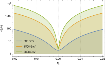
Figure 3: Same as in Fig. 2, but for $F_{3}$.

As the first observable, we consider the total cross-section. Figs. 2 and 3 summarize the total cross-section of the process $\gamma e^{-}\to\tau\bar{\nu}_{\tau}\nu_{e}$ with unpolarized electrons beams and as a function of the anomalous couplings $F_{2}(F_{3})$. We use the three stages of the center-of-mass energy of the CLIC given in Table I. The total cross-section clearly shows a strong dependence with respect to the anomalous parameters $F_{2}$, $F_{3}$, as well as with the center-of-mass energy of the collider $\sqrt{s}$.

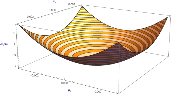
Figure 4: The total cross-sections of the process $\gamma e^{-}\to\tau\bar{\nu}_{\tau}\nu_{e}$ as a function of $F_{2}$ and $F_{3}$ for center-of-mass energy of $\sqrt{s}=380\hskip 2.27621ptGeV$.

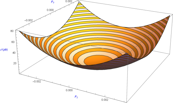
Figure 5: Same as in Fig. 4, but for $\sqrt{s}=1500\hskip 2.27621ptGeV$.

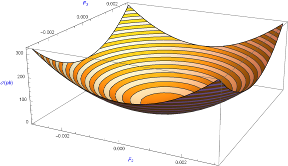
Figure 6: Same as in Fig. 4, but for $\sqrt{s}=3000\hskip 2.27621ptGeV$.

The total cross-section of the process $\gamma e^{-}\to\tau\bar{\nu}_{\tau}\nu_{e}$ as a function of $F_{2}$ and $F_{3}$ with the benchmark parameters of the CLIC given in Table I is shown in Figs. 4-6. The total cross-section increases with the increase in the center-of-mass energy of the collider and strongly depends on anomalous couplings $F_{2}$ and $F_{3}$.

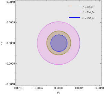
Figure 7: Bounds contours at the $95\%\hskip 2.84526ptC.L.$ in the $F_{3}-F_{2}$ plane for the process $\gamma e^{-}\to\tau\bar{\nu}_{\tau}\nu_{e}$ with the $\delta_{sys}=0\%$ and for center-of-mass energy of $\sqrt{s}=380\hskip 2.27621ptGeV$.

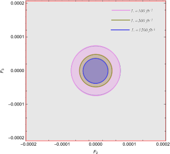
Figure 8: Same as in Fig. 7, but for $\sqrt{s}=1500\hskip 2.27621ptGeV$.

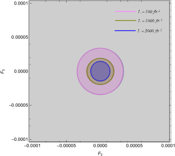
Figure 9: Same as in Fig. 7, but for $\sqrt{s}=3000\hskip 2.27621ptGeV$.

In order to investigate the signal more comprehensively, we show the bounds contours depending on integrated luminosity at the $95\%$ C.L. on the $(F_{2},F_{3})$ plane for $\sqrt{s}=380,1500,3000\hskip 2.27621ptGeV$ in Figs. 7-9. At $95\%$ C.L. and $\sqrt{s}=3000\hskip 2.27621ptGeV$, we can see that the correlation region of $F_{2}\hskip 2.84526pt\in\hskip 2.84526pt[-2.5;2.5]\times 10^{-5}$ and $F_{3}\hskip 2.84526pt\in\hskip 2.84526pt[-2.5;2.5]\times 10^{-5}$ can be excluded with integrate luminosity ${\cal L}=100\hskip 2.27621ptfb^{-1}$. If the integrated luminosity is increased to ${\cal L}=3000\hskip 2.27621ptfb^{-1}$, the excluded region will expand into $F_{2}\hskip 2.84526pt\in\hskip 2.84526pt[-1,1]\times 10^{-5}$ and $F_{3}\hskip 2.84526pt\in\hskip 2.84526pt[-1,1]\times 10^{-5}$.

II.2 Cross-section of the process $\gamma e^{-}\to\tau\bar{\nu}_{\tau}\nu_{e}$ and dipole moments of the $\nu_{\tau}$ with polarized electrons beams

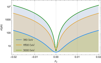
Figure 10: Same as in Fig. 2, but with polarized electron beams $P_{e}=-80\%$.

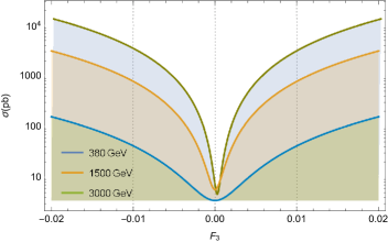
Figure 11: Same as in Fig. 3, but with polarized electron beams $P_{e}=-80\%$.

We consider the total cross-section of the process $\gamma e^{-}\to\tau\bar{\nu}_{\tau}\nu_{e}$ as a function of the anomalous form factors $F_{2}(F_{3})$ and we perform our analysis for the CLIC running at center-of-mass energies and luminosities given in Table I. Furthermore, in our analysis we consider the baseline expectation of an $80\%$ left-polarized electron beam. As expected, the polarization hugely improves the total cross-section as is shown in Figs. 10 and 11. The total cross-section is increased from about $\sigma=8\times 10^{3}\hskip 2.27621ptpb$ with unpolarized electron beam (see Figs. 2 and 3) to about $\sigma=1.5\times 10^{4}\hskip 2.27621ptpb$ with polarized electron beam (see Figs. 10 and 11), respectively, enhancing the statistic. The increase of the total cross-section of the process $\gamma e^{-}\to\tau\bar{\nu}_{\tau}\nu_{e}$ for the polarized case is approximately the double of the unpolarized case. The Feynman diagram 4 of Fig. 1, gives the maximum contribution to the total cross-section. For $P_{e^{-}}=-80\%$ case, this contribution is dominant due to the structure of the $We^{-}\nu_{e^{-}}$ vertex. The advantage of beam polarization is evident when compared to the corresponding unpolarized case.

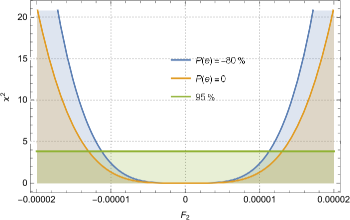
Figure 12: $\chi^{2}$ as a function of $F_{2}$ for the total cross-section of the process $\gamma e^{-}\to\tau\bar{\nu}_{\tau}\nu_{e}$.

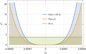
Figure 13: Same as in Fig. 12, but for $F_{3}$.

In Figs. 12 and 13 we plot the $\chi^{2}$ versus $F_{2}(F_{3})$ with unpolarized $P_{e^{-}}=0\%$ and polarized $P_{e^{-}}=-80\%$ electron beam and $95\%\hskip 2.27621ptC.L.$. We plot the curves for each case, for which we have divided the interval of $F_{2}(F_{3})$ into several bins. From these figures we can see that the effect of the polarized beam is to reduce the interval of definition of $F_{2}\hskip 2.84526pt\in\hskip 2.84526pt[-2;2]\times 10^{-5}$ (unpolarized case) to $F_{2}\hskip 2.84526pt\in\hskip 2.84526pt[-1.65;1.65]\times 10^{-5}$ (polarized case) and $F_{3}\hskip 2.84526pt\in\hskip 2.84526pt[-2;2]\times 10^{-5}$ (unpolarized case) to $F_{3}\hskip 2.84526pt\in\hskip 2.84526pt[-1.65;1.65]\times 10^{-5}$ (polarized case), respectively.

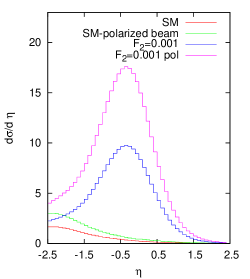
Figure 14: Generated tau-lepton pseudorapidity distribution for $\gamma e^{-}\to\tau\bar{\nu}_{\tau}\nu_{e}$. The distributions are for SM (SM-polarized beam) and $F_{2}$ ($F_{2}$-polarized beam).

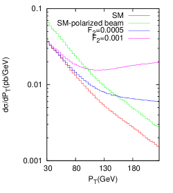
Figure 15: Same as in Fig. 14, but for $P_{T}$.

Another important observable is the transverse momentum $p^{\tau}_{T}$ of the tau lepton, the pseudorapidity $\eta^{\tau}$ is also important, these quantities are shown in Figs. 14 and 15. In both cases, the tau-lepton pseudorapidity and the transverse momentum are for the SM, SM-polarized beam, $F_{2}$ and $F_{2}$-polarized beam. From Fig. 14, the $d\sigma/d\eta$ clearly shows a strong dependence with respect to the pseudorapidity, as well as with the form factors $F_{2}$ and $F_{2}$-polarized beam. In the case of Fig. 15, the distribution $d\sigma/dp_{T}(pb/GeV)$ decreases with the increase of $p_{T}$ for the SM and the SM-polarized beam, while for $F_{2}$ and $F_{2}$-polarized beam have the opposite effect. These distributions clearly show great sensitivity with respect to the anomalous form factor $F_{2}$ for the cases with unpolarized and polarized electron beam. The analysis of these distributions is important to be able to discriminate the basic acceptance cuts for $\tau\bar{\nu}_{\tau}\nu_{e}$ events at the CLIC.

II.3 $90\%$ C.L. and $95\%$ C.L. bounds on the anomalous $\nu_{\tau}$MM and $\nu_{\tau}$EDM with unpolarized and polarized electron beam

In the following we will refer to the anomalous $\nu_{\tau}$MM and $\nu_{\tau}$EDM. From Feynman diagrams for the process $\gamma e^{-}\to\tau\bar{\nu}_{\tau}\nu_{e}$ given in Fig. 1, for the estimation of the sensitivty on the anomalous dipole moments, we consider the following scenarios: a) unpolarized electrons beams $P_{e^{-}}$=0% and we considered only the leptonic decay channel of the tau-lepton. b) polarized electrons beams $P_{e^{-}}$=-80%, and we considered only the leptonic decay channel of the tau-lepton. c) unpolarized electrons beams $P_{e^{-}}$=0% and we considered only the hadronic decay channel of the tau-lepton. d) polarized electrons beams $P_{e^{-}}$=-80% and we considered only the hadronic decay channel of the tau-lepton. For all these scenarios, we consider the energies and luminosities for the future CLIC summarized in Table I. In addition, we imposing kinematic cuts on $p^{\nu}_{T}$, $p^{\tau}_{T}$ and $\eta^{\tau}$ to suppress the backgrounds and to optimize the signal sensitivity (see Eq. (5)), we also consider the systematic uncertainties $\delta_{sys}=0,5,10\%$. The achievable precision in the determination of the sensibility on $\mu_{\nu_{\tau}}$ and the $d_{\nu_{\tau}}$ is summarized in Tables II-IX.

The best sensitivity achieved for the anomalous $\mu_{\nu_{\tau}}$ and the $d_{\nu_{\tau}}$ for the case of $P_{e^{-}}=0\%$, and considering only the leptonic decay channel of the tau-lepton are $|\mu_{\nu_{\tau}}(\mu_{B})|=3.649\times 10^{-7}$ and $|d_{\nu_{\tau}}(ecm)|=7.072\times 10^{-18}$. In the case of $P_{e^{-}}=-80\%$, and considering only the leptonic decay channel of the tau-lepton the sensitivity estimates are $|\mu_{\nu_{\tau}}(\mu_{B})|=3.152\times 10^{-7}$ and $|d_{\nu_{\tau}}(ecm)|=6.108\times 10^{-18}$. In both cases the obtained sensitivity are for the values of $\sqrt{s}=3000\hskip 2.27621ptGeV$, ${\cal L}=3000\hskip 2.27621ptfb^{-1}$ and $95\%$ C.L. Comparing both cases, unpolarized and polarized electron beams, we conclude that the case with polarized beams $P_{e^{-}}=-80\%$ improves the sensitivity on the anomalous dipole moments in $13.63\%$ with respect to the unpolarized case.

When only the hadronic decay channel of the tau-lepton is considered, the sensibility on the dipole moments is $|\mu_{\nu_{\tau}}(\mu_{B})|=3.127\times 10^{-7}$, $|d_{\nu_{\tau}}(ecm)|=6.059\times 10^{-18}$ with $P_{e^{-}}=0\%$ and $|\mu_{\nu_{\tau}}(\mu_{B})|=2.700\times 10^{-7}$, $|d_{\nu_{\tau}}(ecm)|=5.232\times 10^{-18}$ with $P_{e^{-}}=-80\%$, respectively. The obtained results are with $\sqrt{s}=3000\hskip 2.27621ptGeV$, ${\cal L}=3000\hskip 2.27621ptfb^{-1}$ and $95\%$ C.L. The comparison of both cases shows that the case with polarized electron beams improves the sensitivity of the anomalous dipole moments of the $\tau$-neutrino of $13.65\%$, with respect to the case with $P_{e^{-}}=0\%$.

If now we compare the cases with leptonic decay channel and hadronic decay channel with $P_{e^{-}}=0\%$ and $\sqrt{s}=3000\hskip 2.27621ptGeV$, ${\cal L}=3000\hskip 2.27621ptfb^{-1}$ and $95\%$ C.L. the improvement in sensitivity is $14.31\%$ for the hadronic decay channel with respect to the leptonic decay channel. Whereas for $P_{e^{-}}=-80\%$ the improvement in the sensitivity is of $14.34\%$ with respect to the case of the leptonic decay channel. These differences are expected for the different cases because the tau-lepton decays roughly $35\%$ of the time leptonically and $65\%$ of the time hadronically.

III Conclusions

We have studied the $\nu_{\tau}$MM and $\nu_{\tau}$EDM in a model-independent way. For the two options that we considered in this paper: polarized and unpolarized electron beams, our results are sensitive to the parameters of the collider such as the center-of-mass energy and the luminosity. Furthermore, our results are also sensitive to the kinematic basic acceptance cuts of the final states particles $p^{\nu}_{T}$, $\eta^{\tau}$ and $p^{\tau}_{T}$, as well as the systematic uncertainties $\delta_{sys}$. A good knowledge of the kinematic cuts is needed not only to improve sensitivity analyses, but because can help to understand which are the most appropriate processes to probing in the future high-energy and high-luminosity linear colliders, such as the CLIC. CLIC, as well as any $\gamma e^{-}$ Compton backscattering experiment, offers a good laboratory to study the total cross-section and the dipole moments of the tau-neutrino through the process $\gamma e^{-}\to\tau\bar{\nu}_{\tau}\nu_{e}$ with unpolarized and polarized electron beams.

Despite the large number of study performed in recent years on the electromagnetic properties of the tau-neutrino, more studies are still needed to deeply understand and explain experimental observations and their comparison with models predictions. Current and future data of the ATLAS ATLAS and CMS V ; V1 Collaborations, as well as new analysis of already existing data sets, could help to improve our knowledge on the $\nu_{\tau}$MM and $\nu_{\tau}$EDM Gutierrez10 .

A precision machine like CLIC is expected to help in the precise estimates of the anomalous couplings. In this paper, the process $\gamma e^{-}\to\tau\bar{\nu}_{\tau}\nu_{e}$, which contains the neutrino to photon coupling, namely $\nu_{\tau}\bar{\nu}_{\tau}\gamma$ is considered. The reach of the CLIC with maximum $\sqrt{s}=3000\hskip 2.27621ptGeV$ and ${\cal L}=3000\hskip 2.27621ptfb^{-1}$ to probing the relevant observable of the process is presented. The influence of the anomalous couplings, of the kinematic cuts, of the uncertainties systematic, as well as the polarized electron beam on the cross-section, the tau-lepton pseudorapidity distribution and the tau-lepton transverse momentum distribution are studied. Furthermore, we estimates the sensitivity on the anomalous $\nu_{\tau}$MM and $\nu_{\tau}$EDM. Our results are summarized in Figs. 2-15 as well as in Tables II-IX, respectively.

From our set of Figures and Tables it is evident that a suitably chosen beam polarization is found to be advantageous as illustrated with an $80\%$ left-polarization electron beam (see Figs. 10-15). The most optimistic scenario about the sensitivity in the anomalous dipole moments of the tau-neutrino (see Tables V and IX), yields the following results: $|\mu_{\nu_{\tau}}(\mu_{B})|=2.998\times 10^{-7}$ and $|d_{\nu_{\tau}}(ecm)|=5.598\times 10^{-18}$ with $P_{e^{-}}=-80\%$ and we considered only the leptonic decay channel of the tau-lepton. $|\mu_{\nu_{\tau}}(\mu_{B})|=2.475\times 10^{-7}$ and $|d_{\nu_{\tau}}(ecm)|=4.796\times 10^{-18}$, with $P_{e^{-}}=-80\%$ and we taken in account only the hadronic decay channel of the tau-lepton. Our results show the potential and the feasibility of the process $\gamma e^{-}\to\tau\bar{\nu}_{\tau}\nu_{e}$ at the CLIC at the $\gamma e^{-}$ mode.

Acknowledgements

A. G. R. and M. A. H. R acknowledges support from SNI and PROFOCIE (México).

Table 2: Limits on the $\mu_{\nu_{\tau}}$ magnetic moment and $d_{\nu_{\tau}}$ electric dipole moment via the process $\gamma e^{-}\to\tau\bar{\nu}_{\tau}\nu_{e}$ ($\gamma$ is the Compton backscattering photon) for $P_{e^{-}}=0\%$, and we considered only the leptonic decay channel of the tau-lepton.

$90\%\hskip 2.27621ptC.L.$	$\sqrt{s}=1.5\hskip 2.27621ptTeV$
${\cal L}\hskip 2.27621pt(fb^{-1})$	$|\mu_{\nu_{\tau}}|$ ($10^{-7}$)	$|d_{\nu_{\tau}}|$($10^{-17}$)(e cm)
$100$	$16.810$	$3.258$
$200$	$14.130$	$2.739$
$500$	$11.240$	$2.178$
$1000$	$9.455$	$1.832$
$1500$	$8.544$	$1.655$
$\delta_{sys}=5\%$	$6.860\times 10^{-6}$	$1.322\times 10^{-16}$
$\delta_{sys}=10\%$	$9.701\times 10^{-6}$	$1.879\times 10^{-16}$
$95\%\hskip 2.27621ptC.L.$	$\sqrt{s}=1.5\hskip 2.27621ptTeV$
$100$	$18.340$	$3.554$
$200$	$15.420$	$2.989$
$500$	$12.260$	$2.377$
$1000$	$10.310$	$1.999$
$1500$	$9.3210$	$1.806$
$\delta_{sys}=5\%$	$7.484\times 10^{-6}$	$1.450\times 10^{-16}$
$\delta_{sys}=10\%$	$10.580\times 10^{-6}$	$2.051\times 10^{-16}$

Table 3: Limits on the $\mu_{\nu_{\tau}}$ magnetic moment and $d_{\nu_{\tau}}$ electric dipole moment via the process $\gamma e^{-}\to\tau\bar{\nu}_{\tau}\nu_{e}$ ($\gamma$ is the Compton backscattering photon) for $P_{e^{-}}=0\%$, and we considered only the leptonic decay channel of the tau-lepton.

$90\%\hskip 2.27621ptC.L.$	$\sqrt{s}=3\hskip 2.27621ptTeV$
${\cal L}\hskip 2.27621pt(fb^{-1})$	$|\mu_{\nu_{\tau}}|$ ($10^{-7}$)	$|d_{\nu_{\tau}}|$($10^{-18}$)(e cm)
$100$	$7.826$	$15.160$
$500$	$5.234$	$10.140$
$1000$	$4.402$	$8.530$
$2000$	$3.702$	$7.174$
$3000$	$3.345$	$6.483$
$\delta_{sys}=5\%$	$3.029\times 10^{-6}$	$5.871\times 10^{-17}$
$\delta_{sys}=10\%$	$4.248\times 10^{-6}$	$8.233\times 10^{-17}$
$95\%\hskip 2.27621ptC.L.$	$\sqrt{s}=3\hskip 2.27621ptTeV$
$100$	$8.538$	$16.540$
$500$	$5.710$	$11.060$
$1000$	$4.802$	$9.306$
$2000$	$4.038$	$7.826$
$3000$	$3.649$	$7.072$
$\delta_{sys}=5\%$	$3.268\times 10^{-6}$	$6.333\times 10^{-17}$
$\delta_{sys}=10\%$	$4.622\times 10^{-6}$	$8.957\times 10^{-17}$

Table 4: Limits on the $\mu_{\nu_{\tau}}$ magnetic moment and $d_{\nu_{\tau}}$ electric dipole moment via the process $\gamma e^{-}\to\tau\bar{\nu}_{\tau}\nu_{e}$ ($\gamma$ is the Compton backscattering photon) for $P_{e^{-}}=-80\%$, and we considered only the leptonic decay channel of the tau-lepton.

$90\%\hskip 2.27621ptC.L.$	$\sqrt{s}=1.5\hskip 2.27621ptTeV$
${\cal L}\hskip 2.27621pt(fb^{-1})$	$|\mu_{\nu_{\tau}}|$ ($10^{-7}$)	$|d_{\nu_{\tau}}|$($10^{-17}$)(e cm)
$100$	$14.520$	$2.814$
$200$	$12.210$	$2.366$
$500$	$9.713$	$1.882$
$1000$	$8.167$	$1.582$
$1500$	$7.380$	$1.430$
$\delta_{sys}=5\%$	$6.865\times 10^{-6}$	$1.330\times 10^{-16}$
$\delta_{sys}=10\%$	$9.709\times 10^{-6}$	$1.881\times 10^{-16}$
$95\%\hskip 2.27621ptC.L.$	$\sqrt{s}=1.5\hskip 2.27621ptTeV$
$100$	$15.840$	$3.070$
$200$	$13.320$	$2.582$
$500$	$10.590$	$2.053$
$1000$	$8.911$	$1.726$
$1500$	$8.052$	$1.560$
$\delta_{sys}=5\%$	$7.491\times 10^{-6}$	$1.451\times 10^{-16}$
$\delta_{sys}=10\%$	$10.590\times 10^{-6}$	$2.052\times 10^{-16}$

Table 5: Limits on the $\mu_{\nu_{\tau}}$ magnetic moment and $d_{\nu_{\tau}}$ electric dipole moment via the process $\gamma e^{-}\to\tau\bar{\nu}_{\tau}\nu_{e}$ ($\gamma$ is the Compton backscattering photon) for $P_{e^{-}}=-80\%$, and we considered only the leptonic decay channel of the tau-lepton.

$90\%\hskip 2.27621ptC.L.$	$\sqrt{s}=3\hskip 2.27621ptTeV$
${\cal L}\hskip 2.27621pt(fb^{-1})$	$|\mu_{\nu_{\tau}}|$ ($10^{-7}$)	$|d_{\nu_{\tau}}|$($10^{-18}$)(e cm)
$100$	$6.762$	$13.100$
$500$	$4.522$	$8.762$
$1000$	$3.802$	$7.368$
$2000$	$3.197$	$6.196$
$3000$	$2.889$	$5.598$
$\delta_{sys}=5\%$	$3.029\times 10^{-6}$	$5.851\times 10^{-17}$
$\delta_{sys}=10\%$	$4.248\times 10^{-6}$	$8.236\times 10^{-17}$
$95\%\hskip 2.27621ptC.L.$	$\sqrt{s}=3\hskip 2.27621ptTeV$
$100$	$7.377$	$14.290$
$500$	$4.933$	$9.560$
$1000$	$4.148$	$8.039$
$2000$	$3.488$	$6.760$
$3000$	$3.152$	$6.108$
$\delta_{sys}=5\%$	$3.273\times 10^{-6}$	$6.343\times 10^{-17}$
$\delta_{sys}=10\%$	$4.629\times 10^{-6}$	$8.971\times 10^{-17}$

Table 6: Limits on the $\mu_{\nu_{\tau}}$ magnetic moment and $d_{\nu_{\tau}}$ electric dipole moment via the process $\gamma e^{-}\to\tau\bar{\nu}_{\tau}\nu_{e}$ ($\gamma$ is the Compton backscattering photon) for $P_{e^{-}}=0\%$, and we considered only the hadronic decay channel of the tau-lepton.

$90\%\hskip 2.27621ptC.L.$	$\sqrt{s}=1.5\hskip 2.27621ptTeV$
${\cal L}\hskip 2.27621pt(fb^{-1})$	$|\mu_{\nu_{\tau}}|$ ($10^{-7}$)	$|d_{\nu_{\tau}}|$($10^{-17}$)(e cm)
$100$	$14.400$	$2.791$
$200$	$12.110$	$2.347$
$500$	$9.632$	$1.866$
$1000$	$8.098$	$1.569$
$1500$	$7.319$	$1.418$
$\delta_{sys}=5\%$	$6.869\times 10^{-6}$	$1.329\times 10^{-16}$
$\delta_{sys}=10\%$	$9.701\times 10^{-6}$	$1.879\times 10^{-16}$
$95\%\hskip 2.27621ptC.L.$	$\sqrt{s}=1.5\hskip 2.27621ptTeV$
$100$	$15.710$	$3.045$
$200$	$13.210$	$2.560$
$500$	$10.500$	$2.036$
$1000$	$8.837$	$1.712$
$1500$	$7.985$	$1.547$
$\delta_{sys}=5\%$	$7.484\times 10^{-6}$	$1.450\times 10^{-16}$
$\delta_{sys}=10\%$	$10.580\times 10^{-6}$	$2.051\times 10^{-16}$

Table 7: Limits on the $\mu_{\nu_{\tau}}$ magnetic moment and $d_{\nu_{\tau}}$ electric dipole moment via the process $\gamma e^{-}\to\tau\bar{\nu}_{\tau}\nu_{e}$ ($\gamma$ is the Compton backscattering photon) for $P_{e^{-}}=0\%$, and we considered only the hadronic decay channel of the tau-lepton.

$90\%\hskip 2.27621ptC.L.$	$\sqrt{s}=3\hskip 2.27621ptTeV$
${\cal L}\hskip 2.27621pt(fb^{-1})$	$|\mu_{\nu_{\tau}}|$ ($10^{-7}$)	$|d_{\nu_{\tau}}|$($10^{-18}$)(e cm)
$100$	$6.704$	$12.990$
$500$	$4.484$	$8.689$
$1000$	$3.771$	$7.308$
$2000$	$3.171$	$6.146$
$3000$	$2.866$	$5.554$
$\delta_{sys}=5\%$	$2.995\times 10^{-6}$	$5.805\times 10^{-17}$
$\delta_{sys}=10\%$	$4.236\times 10^{-6}$	$8.209\times 10^{-17}$
$95\%\hskip 2.27621ptC.L.$	$\sqrt{s}=3\hskip 2.27621ptTeV$
$100$	$7.314$	$14.170$
$500$	$4.892$	$9.480$
$1000$	$4.114$	$7.972$
$2000$	$3.460$	$6.705$
$3000$	$3.127$	$6.059$
$\delta_{sys}=5\%$	$3.268\times 10^{-6}$	$6.333\times 10^{-17}$
$\delta_{sys}=10\%$	$4.622\times 10^{-6}$	$8.956\times 10^{-17}$

Table 8: Limits on the $\mu_{\nu_{\tau}}$ magnetic moment and $d_{\nu_{\tau}}$ electric dipole moment via the process $\gamma e^{-}\to\tau\bar{\nu}_{\tau}\nu_{e}$ ($\gamma$ is the Compton backscattering photon) for $P_{e^{-}}=-80\%$, and we considered only the hadronic decay channel of the tau-lepton.

$90\%C.L.$	$\sqrt{s}=1.5\hskip 2.27621ptTeV$
Luminosity ($fb^{-1}$)	$|\mu_{\nu_{\tau}}|$ ($10^{-7}$)	$|d_{\nu_{\tau}}|$($10^{-17}$)(e cm)
$100$	$12.440$	$2.411$
$200$	$10.460$	$2.027$
$500$	$8.320$	$1.612$
$1000$	$6.996$	$1.355$
$1500$	$6.322$	$1.225$
$\delta_{sys}=5\%$	$6.865\times 10^{-6}$	$1.330\times 10^{-16}$
$\delta_{sys}=10\%$	$9.709\times 10^{-6}$	$1.881\times 10^{-16}$
$95\%C.L.$	$\sqrt{s}=1.5\hskip 2.27621ptTeV$
$100$	$13.570$	$2.630$
$200$	$11.410$	$2.212$
$500$	$9.078$	$1.759$
$1000$	$7.633$	$1.479$
$1500$	$6.897$	$1.336$
$\delta_{sys}=5\%$	$7.490\times 10^{-6}$	$1.451\times 10^{-16}$
$\delta_{sys}=10\%$	$10.590\times 10^{-6}$	$2.052\times 10^{-16}$

Table 9: Limits on the $\mu_{\nu_{\tau}}$ magnetic moment and $d_{\nu_{\tau}}$ electric dipole moment via the process $\gamma e^{-}\to\tau\bar{\nu}_{\tau}\nu_{e}$ ($\gamma$ is the Compton backscattering photon) for $P_{e^{-}}=-80\%$, and we considered only the hadronic decay channel of the tau-lepton.

$90\%C.L.$	$\sqrt{s}=3\hskip 2.27621ptTeV$
Luminosity ($fb^{-1}$)	$|\mu_{\nu_{\tau}}|$ ($10^{-7}$)	$|d_{\nu_{\tau}}|$($10^{-18}$)(e cm)
$100$	$5.792$	$11.22$
$500$	$3.873$	$7.506$
$1000$	$3.257$	$6.312$
$2000$	$2.739$	$5.307$
$3000$	$2.475$	$4.976$
$\delta_{sys}=5\%$	$3.000\times 10^{-6}$	$5.814\times 10^{-17}$
$\delta_{sys}=10\%$	$4.243\times 10^{-6}$	$8.222\times 10^{-17}$
$95\%C.L.$	$\sqrt{s}=3\hskip 2.27621ptTeV$
$100$	$6.319$	$12.240$
$500$	$4.226$	$8.189$
$1000$	$3.553$	$6.886$
$2000$	$2.988$	$5.791$
$3000$	$2.700$	$5.232$
$\delta_{sys}=5\%$	$3.273\times 10^{-6}$	$6.343\times 10^{-17}$
$\delta_{sys}=10\%$	$4.629\times 10^{-6}$	$8.971\times 10^{-17}$

Figure 2: The total cross-section of the process $\gamma e^{-}\to\tau\bar{\nu}_{\tau}\nu_{e}$ as a function of the anomalous coupling $F_{2}$ for three different center-of-mass energies $\sqrt{s}=380,1500,3000\hskip 2.27621ptGeV$.

References

- (1) S. L. Glashow, Nucl. Phys. 22, 579 (1961).
- (2) S. Weinberg, Phys. Rev. Lett. 19, 1264 (1967).
- (3) A. Salam, in Elementary Particle Theory, Ed. N. Svartholm (Almquist and Wiskell, Stockholm, 1968) 367.
- (4) K. Fujikawa and R. Shrock, Phys. Rev. Lett. 45, 963 (1980).
- (5) Robert E. Shrock, Nucl. Phys. B206, 359 (1982).
- (6) M. Fukugita and T. Yanagida, Physics of Neutrinos and Applications to Astrophysics, (Springer, Berlin, 2003).
- (7) A. Cisneros, Astrophys. Space Sci. 10, 87 (1971).
- (8) M. Zralek, Acta Phys. Polon. B28, 2225 (1997) [hep-ph/9711506].
- (9) A. D. Sakharov, Pisma Zh. Eksp. Teor. Fiz. 5, 32 (1967); JETP Lett. 5, 24 (1967); Sov. Phys. Usp. 34, 392 (1991); Usp. Fiz. Nauk 161, 61 (1991).
- (10) J. H. Christenson, J. W. Cronin, V. L. Fitch, and R. Turlay, Phys. Rev. Lett. 13, 138 (1964).
- (11) K. Abe, et al., Phys. Rev. Lett. 87, 091802 (2001).
- (12) R. Aaij, et al. [LHCb Collaboration], J. High Energy Phys. 07 (2014) 041.
- (13) A. G. Bed, et al., [GEMMA Collaboration] Adv. High Energy Phys. 2012, (2012) 350150.
- (14) L. B. Auerbach, et al., [LSND Collaboration] Phys Rev. D63, (2001) 112001, hep-ex/0101039.
- (15) F. del Aguila and M. Sher, Phys Lett. B252, (1990) 116.
- (16) A. Gutiérrez-Rodríguez, M. Koksal, A. A. Billur, and M. A. Hernández-Ruíz, arXiv:1712.02439 [hep-ph].
- (17) C. Arpesella, et al., [Borexino Collaboration], Phys. Rev. Lett. 101, 091302 (2008).
- (18) R. Schwinhorst, et al., [DONUT Collaboration], Phys. Lett. B513, 23 (2001).
- (19) A. M. Cooper-Sarkar, et al., [WA66 Collaboration], Phys. Lett. B280, 153 (1992).
- (20) M. Acciarri et al., [L3 Collaboration], Phys. Lett. B412, 201 (1997).
- (21) A. Gutiérrez-Rodríguez, M. Koksal and A. A. Billur, Phys. Rev. D91, 093008 (2015).
- (22) A. Llamas-Bugarin, et al., Phys. Rev. D95, 116008 (2017).
- (23) A. Gutiérrez-Rodríguez, Int. J. Theor. Phys. 54, (2015) 236.
- (24) A. Gutiérrez-Rodríguez, Advances in High Energy Physics 2014, 491252 (2014).
- (25) C. Patrignani, et al., [Particle Data Group], Chin. Phys. C40, 100001 (2016).
- (26) A. Gutiérrez-Rodríguez, Pramana Journal of Physics 79, 903 (2012).
- (27) A. Gutiérrez-Rodríguez, Eur. Phys. J. C71, 1819 (2011).
- (28) C. Aydin, M. Bayar and N. Kilic, Chin. Phys. C32, 608 (2008).
- (29) A. Gutiérrez-Rodríguez, et al., Phys. Rev. D74, 053002 (2006).
- (30) A. Gutiérrez-Rodríguez, et al., Phys. Rev. D69, 073008 (2004).
- (31) A. Gutiérrez-Rodríguez, et al., Acta Physica Slovaca 53, 293 (2003).
- (32) K. Akama, T. Hattori and K. Katsuura, Phys. Rev. Lett. 88, 201601 (2002).
- (33) A. Aydemir and R. Sever, Mod. Phys. Lett. A16 7, 457 (2001).
- (34) A. Gutiérrez-Rodríguez, et al., Rev. Mex. de Fís. 45, 249 (1999).
- (35) A. Gutiérrez-Rodríguez, et al., Phys. Rev. D58, 117302 (1998).
- (36) P. Abreu, et al., [DELPHI Collaboration], Z. Phys. C74, 577 (1997).
- (37) R. Escribano and E. Massó, Phys. Lett. B395, 369 (1997).
- (38) T. M. Gould and I. Z. Rothstein, Phys. Lett. B333, 545 (1994).
- (39) H. Grotch and R. Robinet, Z. Phys. C39, 553 (1988).
- (40) I. Sahin, Phys. Rev. D85, 033002 (2012).
- (41) I. Sahin and M. Koksal, JHEP 03, 100 (2011).
- (42) J. F. Nieves, Phys. Rev. D26, 3152 (1982).
- (43) B. Kayser, A. Goldhaber, Phys. Rev. D28, 2341 (1983).
- (44) B. Kayser, Phys. Rev. D30, 1023 (1984).
- (45) P. Vogel and J. Engel, Phys. Rev. D39, 3378 (1989).
- (46) J. Bernabeu, et al., Phys. Rev. D62, 113012 (2000).
- (47) J. Bernabeu, et al., Phys. Rev. Lett. 89, 101802 (2000); Phys. Rev. Lett. 89, 229902 (2002).
- (48) M. S. Dvornikov and A. I. Studenikin, Jour. of Exp. and Theor. Phys. 99, 254 (2004).
- (49) C. Giunti and A. Studenikin, Phys. Atom. Nucl. 72, 2089 (2009).
- (50) C. Broggini, C. Giunti, A. Studenikin, Adv. High Energy Phys. 2012, (2012) 459526.
- (51) I. F. Ginzburg, G. L. Kotkin, V. G. Serbo and V. I. Telnov, Nucl. Instr. and Meth. 205, 47 (1983).
- (52) V. I. Telnov, Nucl. Instr. and Meth. A294, 72 (1990).
- (53) R. H. Milburn, Phys. Rev. Lett. 10, 75 (1963).
- (54) F. R. Arutyunyan and V. A. Tumanyan, Sov. Phys. JETP 17, 1412 (1963).
- (55) E. Accomando, et al. (CLIC Phys. Working Group Collaboration), arXiv: hep-ph/0412251, CERN-2004-005.
- (56) D. Dannheim, P. Lebrun, L. Linssen, et al., arXiv: 1208.1402 [hep-ex].
- (57) H. Abramowicz, et al., (CLIC Detector and Physics Study Collaboration), arXiv:1307.5288 [hep-ex].
- (58) A. Belyaev, N. D. Christensen and A. Pukhov, Comput. Phys. Commun. 184, 1729 (2013).
- (59) M. Köksal, A. A. Billur and A. Gutiérrez-Rodríguez, Adv. High Energy Phys. 2017, 6738409 (2017).
- (60) Y. Özgüven, S. C. Inan, A. A. Billur, M. Köksal, M. K. Bahar, Nucl. Phys. B923, 475 (2017).
- (61) M. Köksal, S. C. Inan, A. A. Billur, M. K. Bahar, Y. Özgüven, arXiv:1711.02405 [hep-ph].
- (62) M. Köksal, A. A. Billur, A. Gutiérrez-Rodríguez and M. A. Hernández-Ruíz, arXiv:1804.02373 [hep-ph].
- (63) A. A. Billur, M. Köksal, Phys. Rev. D89, 037301 (2014).
- (64) T. H. Tran, V. Balagura, V. Boudry, J. C. Brient, H. Videau, Eur. Phys. J. C76, 468 (2016).
- (65) M. Aicheler, et al., (editors), A Multi-TeV Linear Collider based on CLIC Technology: CLIC Conceptual Design Report, JAI-2012-001, KEK Report 2012-1, PSI-12-01, SLAC-R-985, https://edms.cern.ch/document/1234244/.
- (66) L. Linssen, et al., (editors),Physics and Detectors at CLIC: CLIC Conceptual Design Report, 2012, ANL-HEP-TR-12-01, CERN-2012-003, DESY 12-008, KEK Report 2011-7, arXiv:1202.5940.
- (67) G. Moortgat-Pick, et al., Physics Reports 460, 131243 (2008).
- (68) V. Ari, A. A. Billur, S. C. Inan and M. Koksal, Nucl. Phys. B906, 211 (2016).
- (69) G. Aad, et al., [ATLAS Collaboration], Phys. Rev. D93, 112002 (2016).
- (70) V. Khachatryan, et al., [CMS Collaboration], Phys. Lett. B760, 448 (2016).
- (71) V. Khachatryan, et al., [CMS Collaboration], JHEP 04, 164 (2015).