Piezoelectric mimicry of flexoelectricity

Abstract

The origin of “giant” flexoelectricity, orders of magnitude larger than theoretically predicted, yet frequently observed, is under intense scrutiny. There is mounting evidence correlating giant flexoelectric-like effects with parasitic piezoelectricity, but it is not clear how piezoelectricity (polarization generated by strain) manages to imitate flexoelectricity (polarization generated by strain gradient) in typical beam-bending experiments, since in a bent beam the net strain is zero. In addition, and contrary to flexoelectricity, piezoelectricity changes sign under space inversion, and this criterion should be able to distinguish the two effects and yet “giant” flexoelectricity is insensitive to space inversion, seemingly contradicting a piezoelectric origin. Here we show that, if a piezoelectric material has its piezoelectric coefficient be asymmetrically distributed across the sample, it will generate a bending-induced polarization impossible to distinguish from “true” flexoelectricity even by inverting the sample. The effective flexoelectric coefficient caused by piezoelectricity is functionally identical to, and often larger than, intrinsic flexoelectricity: the calculations show that, for standard perovskite ferroelectrics, even a tiny gradient of piezoelectricity (1% variation of piezoelectric coefficient across 1 mm) is sufficient to yield a giant effective flexoelectric coefficient of 1 $\mu$C/m, three orders of magnitude larger than the intrinsic expectation value.

Flexoelectricity is attracting growing attention due to its ability to replicate the electromechanical functionality of piezoelectric materials, which opens up the possibility of using lead-free dielectrics as flexoelectric replacements for piezoelectrics in specific applicationsChu et al. (2009); Bhaskar et al. (2016). Experimental research on this phenomenon is still in a relative infancy, but already there have been controversies about the real magnitude, origin and even thermodynamic reversibility of the flexoelectric effect Yudin and Tagantsev (2013); Zubko et al. (2013); Nguyen et al. (2013). Some of these controversies are starting to get settled, and, in particular, there is by now abundant evidence and growing consensus that seemingly “giant” flexoelectric effects are correlated with parasitic piezoelectric contributions from polar nanoregions Narvaez and Catalan (2014), defect concentration gradients Biancoli et al. (2015), residual ferroelectricity Garten and Trolier-McKinstry (2015), or surfaces Tagantsev (1986); Narvaez et al. ; Narvaez et al. (2016). But, while the recent evidence suggests that indeed piezoelectricity can mimic flexoelectricity (which is the converse of flexoelectricity replicating piezoelectricity), it is not clear how (i.e., what are the necessary conditions for piezoelectricity to be able to imitate flexoelectricity), nor to what extent is the “disguise” perfect, i.e., can intrinsic flexoelectricity and flexoelectric-like piezoelectricity be experimentally distinguished?

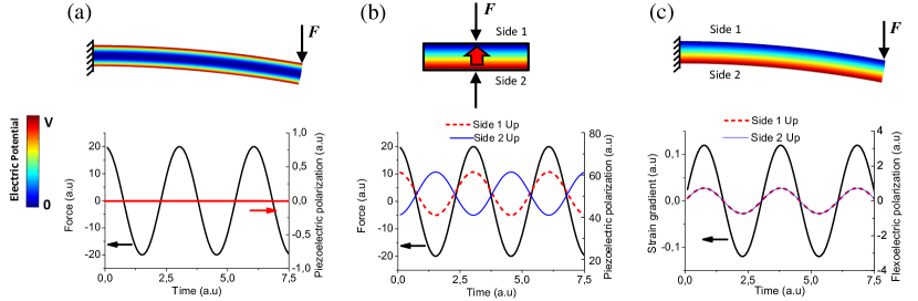
Figure 1: (a) Homogeneously poled piezoelectric beam under bending, which does not induce a non-zero net polarization because the average strain is zero. The color plot presents the electric potential distribution. (b) Piezoelectric polarization induced in a rectangular sample under tension or compression. The red arrow represents the direction of the material polarization. (c) Flexoelectric polarization induced in a cantilever beam under bending. The polarization does not change sign by reversing the beam.

To illustrate these questions, consider the following example: polarization can be generated by flexoelectricity when the applied deformation is inhomogeneous, e.g., when a sample is bent Bursian and Zaikovskii (1968); Ma and Cross (2005); Cross (2006); Zubko et al. (2007); Majdoub et al. (2008); Kwon et al. (2014), but this is not necessarily true for piezoelectricity: bending a homogeneously poled piezoelectric beam will not elicit any piezoelectric polarization, see Fig. 1 (a), because there is no net strain: the piezoelectric polarization caused by stretching on the convex side will be canceled by the opposite polarization caused by compression on the concave side. It follows from this example that the apparently giant flexoelectricity measured in the bending of some materials cannot be caused by a homogeneous piezoelectric state, even if the sample is macroscopically polar Biancoli et al. (2015). Furthermore, because the existence of macroscopic piezoelectricity can be established by space-inversion experiments such as flipping the sample upside-down and verifying that the sign of the stress-generated charge changes sign Biancoli et al. (2015), see Fig. 1 (b), it was assumed that such space-inversion tests could be used to distinguish between piezoelectricity and flexoelectricity Narvaez et al. . Indeed, the bending-induced polarization of a flexoelectric cantilever is independent of its orientation, see Fig. 1(c), but, as we will see, this inversion invariance can also hold for bent piezoelectric cantilevers.

Here, we analyze the electromechanical response of a bent piezoelectric beam, one of the common setups to quantify flexoelectricity Zubko et al. (2013), and show that (i) it is a necessary and sufficient condition that the piezoelectric coefficient be asymmetrically distributed for the beam to be able to replicate the functional behavior of a flexoelectric and (ii) that such asymmetric piezoelectricity cannot be distinguished from flexoelectricity in beam-bending experiments, even if the sample is turned upside down; the disguise is, in this respect, perfect. It is also possible to define an effective flexoelectric constant as a function of the spatial distribution of piezoelectricity. Quantitative analysis of this piezo-flexoelectric coefficient shows that even a relatively modest asymmetry in the distribution of piezoelectricity can lead to an effectively giant flexoelectric effect.

The constitutive equation for the electric displacement $\mathbf{D}$ in a linear dielectric solid possessing piezoelectricity and flexoelectricity is

$$D_{i}=e_{ikl}\varepsilon_{kl}+\mu_{ijkl}\nabla_{l}\varepsilon_{jk}+\epsilon_{ij}E_{j}=\epsilon_{0}E_{i}+P_{i},$$ (1)

where $\mathbf{E}$ is the electric field, $\mathbf{\varepsilon}$ is the mechanical strain, $\mathbf{P}$ is the polarization, $\nabla\mathbf{\varepsilon}$ is the strain gradient, $\mathbf{e}$ is the piezoelectric tensor, $\mathbf{\mu}$ is the flexoelectric tensor, $\mathbf{\epsilon}$ is the dielectric tensor, and $\epsilon_{0}$ is the permittivity of vacuum or air. We begin by analyzing the response of a piezoelectric flexoelectric cantilever beam under bending, see Fig. 2(a). We assume that the electric field and polarization exist only in the beam thickness direction ($z$) since it has been shown that the longitudinal electric filed is negligible compared with that in the beam thickness direction Gao and Wang (2007); Wang and Feng (2010). Then, Eq. (1) simplifies to

$$D_{z}=e_{31}\varepsilon_{xx}+\mu_{13}\varepsilon_{xx,z}+\epsilon_{33}E_{z}=\epsilon_{0}E_{z}+P_{z},$$ (2)

where the notations $e_{311}=e_{31}$ and $\mu_{1331}=\mu_{13}$ are introduced for convenience.

In the absence of surface charges and applied voltage, the electrostatic equilibrium (Maxwell’s equation) leads to

$$D_{z}=\epsilon_{0}E_{z}+P_{z}=0.$$ (3)

Plugging this equation in Eq. (2) and using the Euler beam hypotheses $\varepsilon_{xx}=-\kappa z$ and $\varepsilon_{xx,z}=-\kappa$, where $\kappa$ is the beam curvature induced by the applied force $F$, the polarization in $z$ direction can be obtained as

$$P_{z}(z)=-\frac{\kappa}{\epsilon_{r}}(e_{31}z+\mu_{13}),$$ (4)

where $\epsilon_{r}=\epsilon_{33}/\epsilon_{0}$ is the relative dielectric constant. We note that this equation can also be derived from analytical solutions of the electroelastic fields in bending piezoelectric cantilever beams with the flexoelectric effect Majdoub et al. (2008, 2009); Yan and Jiang (2013) or gradient piezoelectricity Williams (1982, 1983). The total net polarization over the beam thickness is then obtained as

$$P_{t}=\frac{1}{h}\int_{-h/2}^{h/2}P_{z}dz=-\frac{\kappa}{h\epsilon_{r}}\int_{-h/2}^{h/2}(e_{31}z+\mu_{13})dz.$$ (5)

In the absence of piezoelectricity, i.e. $e_{31}=0$, the polarization is only induced by the flexoelectric effect, resulting in a net polarization $P_{t}=-\mu_{13}\kappa/\epsilon_{r}$, independent of the beam direction. In other words, the net polarization induced by flexoelectricity does not change sign by reversing the beam, as expected.

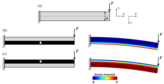
Figure 2: (a) Schematic of a cantilever beam under the point load $F$. (b) Schematic of a bimorph cantilever beam where the dark layer is piezoelectric. (c) A reversed configuration of the bimorph (rotated by 180^o). The white arrows represent the polarization direction of the layers. The color plot presents the electric potential ($\phi$) distribution for each bimorph obtained from Eqs. (3) and (4), where $E_{z}=-\phi_{,z}$. The net polarization can be obtained from the electric potential difference of the top and bottom faces, which is identical in both bimorphs.

We can also use Eq. (5) to obtain the net polarization corresponding to a beam where the electromechanical response is piezoelectric instead of flexoelectric, i.e. $\mu_{13}=0$. However, bending a homogeneous piezoelectric beam is unable to produce a non-zero net polarization since $e_{31}z$ is antisymmetric about the centre of the beam ($z$ = 0), thus leading to a zero net polarization in Eq. (5), see Fig. 1(a). The physical reason, as mentioned at the introduction, is that opposite stresses (compressive and tensile) are induced in the upper and lower halves of the beam respectively, resulting in opposite piezoelectric effects and a zero net polarization. Therefore, bending a homogeneous piezoelectric beam cannot give a flexoelectric-like response.

One way to break the balance of charges in a bent piezoelectric beam is to replace the top or bottom layers with a different piezoelectric or even a non-piezoelectric layer, as is done for example in piezoelectric bimorph sensors and actuators Smits et al. (1991); Pritchard et al. (2001). One such bimorph is illustrated in Fig. 2(b), in which the bottom layer is piezoelectric while the top layer is not, i.e. $e_{31}=0$ for $h\geq 0$ and $e_{31}=-e_{31}$ for $h<0$. The bimorph can be seen as an extreme case of asymmetric piezoelectricity, where $e_{31}$ is a Heaviside step function. In this case the net polarization is obtained from Eq. (5) as $P_{t}$ = $-e_{31}h\kappa/8\epsilon_{r}$.

A bimorph piezoelectric cantilever thus generates a polarization just like a flexoelectric cantilever would. Moreover, the sign (phase shift) of the piezoelectric polarization does not change by reversing the beam. Figure 2(c) presents the reversed configuration which is equivalent to consider $e_{31}=0$ for $h<0$. Plugging these conditions in Eq. (5) leads to a net polarization $P_{t}$ = $-e_{31}h\kappa/8\epsilon_{r}$, identical both in magnitude and sign, to the induced polarization in the original bimorph in Fig. 2(b). Therefore, a bent piezoelectric bimorph is qualitatively indistinguishable from a bent flexoelectric beam.

We can generalize the conclusions of this example. Let us assume a generic cantilever beam with an arbitrary distribution of piezoelectricity $e_{31}(z)$. Equation (5) results in a zero net polarization if the piezoelectricity is symmetrically distributed about the centre of the beam, i.e. for any $e_{31}(z)$ such that $e_{31}(z)=e_{31}(-z)$. Mathematically the integrand is antisymmetric about the centre of the beam for any such symmetrical distribution of piezoelectricity. Conversely, any asymmetry in the distribution of piezoelectricity such that $e_{31}(z)\neq e_{31}(-z)$ will result in a non-zero integral and thus in a net bending-induced piezoelectric polarization.

In addition, the sign of the net polarization in Eq. (5) does not change by flipping the beam. In the flipped configuration, the coordinate system $x-z$ converts to the new system $x^{\prime}-z^{\prime}$, where $z^{\prime}=-z$. Using this conversion and taking into account the negative sign of $e_{31}$ in the flipped configuration, Eq. (5) converts to an identical equation as a function of $z^{\prime}$, retaining its sign. Therefore, for a piezoelectric beam to be able to indistinguishably mimic a flexoelectricity (i.e., for Eq. (5) to yield a non-zero solution that is invariant with respect to space inversion), it is necessary and sufficient that the piezoelectric coefficient be asymmetrically distributed across the thickness of the beam. Two particular embodiments of this general concept are the bimorph piezoelectric cantilever, for which $e_{31}(z)$ is a step-function, and surface piezoelectricity Tagantsev and Yurkov (2012); Zubko et al. (2013); Stengel (2014); Narvaez et al. , for which $e_{31}(z)$ can be viewed as two step functions.

Since an asymmetric piezoelectric can identically mimic a flexoelectric-like response, it is possible to define an effective flexoelectric constant as a function of the distribution of piezoelectricity. For a flexoelectric cantilever, the induced polarization as a function of the beam curvature is given by $P_{t}=-\mu_{e}\kappa/\epsilon_{r}$, where $\mu_{e}$ is the effective flexoelectric constant. By equating this polarization to Eq. (5) with $\mu_{13}=0$, the effective flexoelectric constant becomes

$$\mu_{e}\equiv\frac{1}{h}\int_{-h/2}^{h/2}{e}_{31}(z)zdz.$$ (6)

In order to get some quantitative estimates of how much “pseudo-flexoelectricity” can we elicit from a gradient of piezoelectricity, we consider a simple linear distribution of piezoelectricity as $e_{31}(z)=z{\Delta e}/h+e_{0}$, where $\Delta e/h$ is the slope of the linear gradient of piezoelectricity and $e_{0}=e_{31}(0)$. Plugging this function in Eq. (6) yields an effective flexoelectric coefficient of

$$\mu_{e}=h\Delta e/12.$$ (7)

Let us use this equation to analyze relevant experimental cases. Experimental setups to quantify flexoelectricity commonly employ cantilever beams with a thickness in the order of $h=1$ mm Ma and Cross (2001, 2002, 2005, 2006); Cross (2006); Shu et al. (2013), so their piezoelectrically-induced flexoelectricity would be $\mu_{e}\approx\Delta e\times 10^{-4}$. Therefore, to induce a typical “giant” flexoelectric coefficient in the order of $\mu_{e}=$ 1 $\mu$ C/m, as reported for important piezoelectric materials such as PZT and BaTiO₃ Ma and Cross (2005); Cross (2006); Ma and Cross (2006), the piezoelectric variation $\Delta e$ between the two sides of the 1 mm sample should be in the order of $10^{-2}$ C/m². Compared to the average piezoelectric coefficient of PZT and BaTiO₃, which is in the order of 5 C/m² Li et al. (1991); Zhu et al. (1998), this gradient is equivalent to a 0.2 % change of the piezoelectric constant across the beam thickness. Therefore, for materials with big piezoelectric coefficients, even a tiny gradient of piezoelectricity can yield an apparently giant flexoelectricity. This invalidates bending-based quantifications of flexoelectricity in the polar phase of these materials and highlights the need for alternative experimental approaches Cordero-Edwards et al. (2017).

Another relevant question, of course, is to what extent these results can be extended to nominally paraelectric materials. As has recently been reported, even in a theoretically paraelectric material, an asymmetric distribution of defects can result in a small but measurable macroscopic piezoelectricity Biancoli et al. (2015). The reported effective piezoelectric coefficients for paraelectric perovskites is in the order of 0.05 C/m². Compared to this average value, the same piezoelectric gradient of $10^{-2}$ C/m² across 1 mm required to yield $\mu_{e}=$ 1 $\mu$ C/m represents to 20% variation of the effective piezoelectric constant across the 1 mm thick beam. Though this gradient is large, it is not unrealistic.

The present analysis shows that piezoelectricity can indeed imitate flexoelectricity (bending-induced polarization) on the condition that the piezoelectric coefficient be inhomogeneously and asymmetrically distributed across the sample. If this condition is met, however, asymmetric piezoelectricity - as might be found in bimorphs, but also as provided by surface piezoelectricity Tagantsev and Yurkov (2012); Stengel (2014); Narvaez et al. - becomes functionally indistinguishable from intrinsic flexoelectricity. This perfect mimicry complicates the task of interpreting experimental results in flexoelectricity, but perhaps it also represents a practical opportunity; just like flexoelectricity was initially conceived as a way for replicating the device functionality of piezoelectrics Zhu et al. (2006); Fu et al. (2007); Chu et al. (2009), asymmetric piezoelectricity may be used to imitate the interesting novel functionalities Lu et al. (2012); Starkov and Starkov (2016); Cordero-Edwards et al. (2017); Yang et al. (2018) provided by flexoelectricity.

This research was funded by an ERC Starting grant (ERC 308023). All research in ICN2 is supported by the Severo Ochoa Excellence Programme (SEV-2013-0295) and funded by the CERCA Programme / Generalitat de Catalunya. F.V. thanks UCR, MICITT and CONICIT for support during his PhD.

References

- Chu et al. (2009) B. Chu, W. Zhu, N. Li, and L. E. Cross, J. Appl. Phys. 106, 104109 (2009).
- Bhaskar et al. (2016) U. K. Bhaskar, N. Banerjee, A. Abdollahi, Z. Wang, D. G. Schlom, G. Rijnders, and G. Catalan, Nature Nanotech. 11, 263 (2016).
- Yudin and Tagantsev (2013) P. V. Yudin and A. K. Tagantsev, Nanotech. 24, 432001 (2013).
- Zubko et al. (2013) P. Zubko, G. Catalan, and A. K. Tagantsev, Annu. Rev. Mater. Res. 43, 387 (2013).
- Nguyen et al. (2013) T. D. Nguyen, S. Mao, Y.-W. Yeh, P. K. Purohit, and M. C. McAlpine, Adv. Mater. 25, 946 (2013).
- Narvaez and Catalan (2014) J. Narvaez and G. Catalan, Appl. Phys. Lett. 104, 162903 (2014).
- Biancoli et al. (2015) A. Biancoli, C. Fancher, J. Jones, and D. Damjanovic, Nature Mater. 14, 224 (2015).
- Garten and Trolier-McKinstry (2015) L. M. Garten and S. Trolier-McKinstry, J. Appl. Phys. 117 (2015).
- Tagantsev (1986) A. K. Tagantsev, Phys. Rev. B 34, 5883 (1986).
- (10) J. Narvaez, S. Saremi, J. Hong, M. Stengel, and G. Catalan, Phys. Rev. Lett. 115, 037601.
- Narvaez et al. (2016) J. Narvaez, F. Vasquez-Sancho, and G. Catalan, Nature 538, 219 (2016).
- Bursian and Zaikovskii (1968) E. V. Bursian and O. I. Zaikovskii, Sov. Phys. Solid State 10, 1121 (1968).
- Ma and Cross (2005) W. Ma and L. E. Cross, Appl. Phys. Lett. 86, 072905 (2005).
- Cross (2006) L. E. Cross, J. Mater. Sci. 41, 53 (2006).
- Zubko et al. (2007) P. Zubko, G. Catalan, P. R. L. Welche, A. Buckley, and J. F. Scott, Phys. Rev. Lett. 99, 167601 (2007).
- Majdoub et al. (2008) M. S. Majdoub, P. Sharma, and T. Cagin, Phys. Rev. B 77, 125424 (2008).
- Kwon et al. (2014) S. Kwon, W. Huang, L. Shu, F.-G. Yuan, J.-P. Maria, and X. Jiang, Appl. Phys. Lett. 105 (2014).
- Gao and Wang (2007) Y. Gao and Z. L. Wang, Nano Letters 7, 2499 (2007).
- Wang and Feng (2010) G.-F. Wang and X.-Q. Feng, Europhys. Lett. Assoc. 91, 56007 (2010).
- Majdoub et al. (2009) M. S. Majdoub, P. Sharma, and T. Cagin, Phys. Rev. B 79, 119904(E) (2009).
- Yan and Jiang (2013) Z. Yan and L. Y. Jiang, J. Appl. Phys. 113, 194102 (2013).
- Williams (1982) W. S. Williams, Ferroelectrics 41, 225 (1982).
- Williams (1983) W. S. Williams, Ferroelectrics 51, 61 (1983).
- Smits et al. (1991) J. G. Smits, S. I. Dalke, and T. K. Cooney, Sens. Actuators A: Phys. 28, 41 (1991).
- Pritchard et al. (2001) J. Pritchard, C. R. Bowen, and F. Lowrie, British Ceram. Trans. 100, 265 (2001).
- Tagantsev and Yurkov (2012) A. K. Tagantsev and A. S. Yurkov, J. Appl. Phys. 112, 044103 (2012).
- Stengel (2014) M. Stengel, Phys. Rev. B 90, 201112 (2014).
- Ma and Cross (2001) W. Ma and L. E. Cross, Appl. Phys. Lett. 79, 4420 (2001).
- Ma and Cross (2002) W. Ma and L. E. Cross, Appl. Phys. Lett. 81, 3440 (2002).
- Ma and Cross (2006) W. Ma and L. E. Cross, Appl. Phys. Lett. 88, 232902 (2006).
- Shu et al. (2013) L. Shu, X. Wei, L. Jin, Y. Li, H. Wang, and X. Yao, Appl. Phys. Lett. 102, 152904 (2013).
- Li et al. (1991) Z. Li, S. K. Chan, M. H. Grimsditch, and E. S. Zouboulis, J. Appl. Phys. 70, 7327 (1991).
- Zhu et al. (1998) S. Zhu, B. Jiang, and W. Cao, Proc. SPIE 3341, 154 (1998).
- Cordero-Edwards et al. (2017) K. Cordero-Edwards, N. Domingo, A. Abdollahi, J. Sort, and G. Catalan, Adv. Mater. 29, 1702210 (2017).
- Zhu et al. (2006) W. Zhu, J. Y. Fu, N. Li, and L. Cross, Appl. Phys. Lett. 89, 192904 (2006).
- Fu et al. (2007) J. Y. Fu, W. Zhu, N. Li, N. B. Smith, and L. E. Cross, Appl. Phys. Lett. 91, 182910 (2007).
- Lu et al. (2012) H. Lu, C. W. Bark, D. E. D. L. Ojos, J. Alcala, C. B. Eom, G. Catalan, and A. Gruverman, Science 335, 59 (2012).
- Starkov and Starkov (2016) A. S. Starkov and I. A. Starkov, Int. J. Solids and Struct. 82, 65 (2016).
- Yang et al. (2018) M.-M. Yang, D. J. Kim, and M. Alexe, Science (2018), 10.1126/science.aan3256.