Game-Theoretic Interpretability for Temporal Modeling

Abstract

Interpretability has arisen as a key desideratum of machine learning models alongside performance. Approaches so far have been primarily concerned with fixed dimensional inputs emphasizing feature relevance or selection. In contrast, we focus on temporal modeling and the problem of tailoring the predictor, functionally, towards an interpretable family. To this end, we propose a co-operative game between the predictor and an explainer without any a priori restrictions on the functional class of the predictor. The goal of the explainer is to highlight, locally, how well the predictor conforms to the chosen interpretable family of temporal models. Our co-operative game is setup asymmetrically in terms of information sets for efficiency reasons. We develop and illustrate the framework in the context of temporal sequence models with examples.

1 Introduction

State-of-the-art predictive models tend to be complex and involve a very large number of parameters. While the added complexity brings modeling flexibility, it comes at the cost of transparency or interpretability. This is particularly problematic when predictions feed into decision-critical applications such as medicine where understanding of the underlying phenomenon being modeled may be just as important as raw predictive power.

Previous approaches to interpretability have focused mostly on fixed-size data, such as scalar-feature datasets (Lakkaraju et al., 2016) or image prediction tasks (Selvaraju et al., 2016). Recent methods do address the more challenging setting of sequential data (Lei et al., 2016; Arras et al., 2017) in NLP tasks where the input is discrete. Interpretability for continuous temporal data has remained mostly unexplored (Wu et al., 2018).

In this work, we propose a novel approach to model interpretability that is naturally tailored (though not limited to) time-series data. Our approach differs from interpretable models such as interpretation generators (Al-Shedivat et al., 2017; Lei et al., 2016) where the architecture or the function class is itself explicitly constrained towards interpretability, e.g., taking it to be the set of linear functions. We also differ from post-hoc explanations of black-box methods through local perturbations (Ribeiro et al., 2016; Alvarez-Melis & Jaakkola, 2017). In contrast, we establish an intermediate regime, game-theoretic interpretability, where the predictor remains functionally complex but is encouraged during training to follow a locally interpretable form.

At the core of our approach is a game-theoretic characterization of interpretability. This is set up as a two-player co-operative game between predictor and explainer. The predictor remains a complex model whereas the explainer is chosen from a simple interpretable family. The players minimize asymmetric objectives that combine the prediction error and the discrepancy between the players. The resulting predictor is biased towards agreeing with a co-operative explainer. The co-operative game equilibrium is stable in contrast to GANs (Goodfellow et al., 2014).

The main contributions of this work are as follows:

• A novel game-theoretic interpretability framework that can take a wide range of prediction models without architectural modifications.

• Accurate yet explainable predictors where the explainer is trained coordinately with the predictor to actively balance interpretability and accuracy.

• Interpretable temporal models, validated through quantitative and qualitative experiments, including stock price prediction and a physical component modeling.

2 Methodology

In this work, we learn a (complex) predictive target function $f\in\mathcal{F}:\mathcal{X}\to\mathcal{Y}$ together with a simpler function $g\in\mathcal{G}:\mathcal{X}\to\mathcal{Y}$ defined over an axiomatic class of interpretable models $\mathcal{G}$. We refer to functions $f$ and $g$ as the predictor and explainer, respectively, throughout the paper. Note that we need not make any assumptions on the function class $\mathcal{F}$, instead allowing a flexible class of predictors. In contrast, the family of explainers $\mathcal{G}$ is explicitly and intentionally constrained such as the set of linear functions. As any $g\in\mathcal{G}$ is assumed to be interpretable, the family $\mathcal{G}$ does not typically itself suffice to capture the regularities in the data. We can therefore hope to encourage the predictor to remain close to such interpretable models only locally.

For expository purposes, we will develop the framework in a discrete time setting where the predictor maps $x_{t}\in\mathcal{X}$ to $f(x_{t})\in\mathcal{Y}$ for $t=\{1,2,\dots\}$. The data are denoted as $\mathcal{D}=\{(x_{1},y_{1}),(x_{2},y_{2}),\dots\}$. We then instantiate the predictor with deep sequence generative models, and the explainers with linear models.

2.1 Game-Theoretic Interpretability

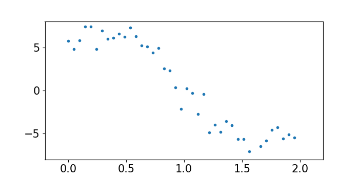
(a) Neighborhood $\mathcal{B}_{\epsilon}(x_{t}=1)$

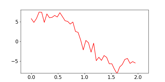
(b) Piece-wise linear $f$

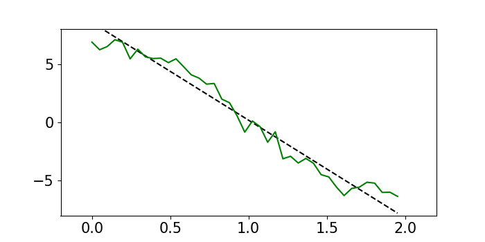
(c) $g_{x_{t}}\in\mathcal{G}_{\text{Linear}}$

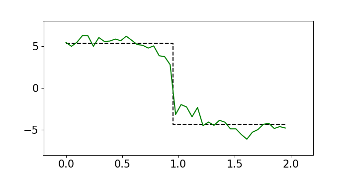
(d) $g_{x_{t}}\in\mathcal{G}_{\text{Decision Stump}}$

Figure 1: Examples of fitting a neighborhood $\mathcal{B}_{\epsilon}(x_{t}=1)$ (1(a)) with piece-wise linear predictor (1(b)). When playing with different families of explainers (Figure 1(c) and 1(d); dashed lines), the resulting predictor (in solid green) behaves differently although they admit the same prediction error (mean squared error = 1.026).

There are many ways to use explainer functions $g\in\mathcal{G}$ to guide the predictor $f$ by means of discrepancy measures. However, since the explainer functions are inherently weak such as linear functions, we cannot expect that a reasonable predictor would be nearly linear globally. Instead, we can enforce this property only locally. To this end, we define local interpretability by measuring how close $f$ is to a family $\mathcal{G}$ over a local neighborhood $\mathcal{B}_{\epsilon}(x_{t})$ around an observed point $x_{t}$. One straightforward instantiation of such a neighborhood $\mathcal{B}_{\epsilon}({x_{t}})$ in temporal modeling will be simply a local window of points $\{x_{t-\epsilon},\dots,x_{t+\epsilon}\}$. Our resulting local discrepancy measure is

$$\min_{g\in\mathcal{G}}d_{x_{t}}(f,g)=\min_{g\in\mathcal{G}}\frac{\sum_{x^{\prime}\in\mathcal{B}_{\epsilon}(x_{t})}d(f(x^{\prime}),g(x^{\prime}))}{|\mathcal{B}_{\epsilon}({x_{t}})|},\vspace{1mm}$$ (1)

where $d(\cdot,\cdot)$ is a deviation measurement. The minimizing explainer function, $\hat{g}_{x_{t}}$, is indexed by the point $x_{t}$ around which it is estimated. Indeed, depending on the function $f$, the minimizing explainer can change from one neighborhood to another. If we view the minimization problem game-theoretically, $\hat{g}_{x_{t}}$ is the best response strategy of the local explainer around $x_{t}$.

The local discrepancy measure can be subsequently incorporated into an overall regularization problem for the predictor either symmetrically (shared objective) or asymmetrically (game-theoretic) where the goals differ between the predictor and the explainer.

Symmetric criterion. Assume that we are given a primal loss $\mathcal{L}(\cdot,\cdot)$ that is to be minimized for the problem of interest. The goal of the predictor is then to find $f$ that offers the best balance between the primal loss and local interpretability. Due to the symmetry between the two players, the full game can be collapsed into a single objective

$$\sum_{(x_{t},y_{t})\in\mathcal{D}}\bigg{[} \mathcal{L}(f(x_{t}),y_{t})$$

$$+\frac{\lambda}{|\mathcal{B}_{\epsilon}(x_{t})|}\sum_{x^{\prime}\in\mathcal{B}_{\epsilon}(x_{t})}d(f(x^{\prime}),g_{x_{t}}(x^{\prime}))\bigg{]}$$ (2)

to be minimized with respect to both $f$ and $g_{x_{t}}$. Here, $\lambda$ is a hyper-parameter that we have to set.

To illustrate the above idea, we generate a synthetic dataset to show a neighborhood in Figure 1(a) with a perfect piece-wise linear predictor $f\in\mathcal{F_{\text{Piece-wise Linear}}}$ in Figure 1(b). Clearly, $f$ does not agree with linear explainers within the neighborhood, despite its piece-wise linear nature. However, when we establish a game between $f$ and a linear explainer $g_{x_{t}=1}\in\mathcal{G}_{\text{Linear}}$ in Figure 1(c), it admits lower functional deviation (and thus stronger linear interpretability). We also show in Figure 1(d) that different explainer family would induce different outcomes of the game.

Asymmetric Game. The symmetric criterion makes it simple to understand the overall co-operative objective, but solving it is inefficient computationally. Different possible sizes of the neighborhood $\mathcal{B}_{\epsilon}(x)$ (e.g., end-point boundary cases) makes it hard to parallelize optimization for $f$ (note that this does not hold for $g_{x_{t}}$), which is problematic when we require parallel training for neural networks. Also, since $f$ is reused many times across neighborhoods in the discrepancy measures, the value of $f$ at each $x_{t}$ may be subject to different functional regularization across the neighborhoods, which is undesirable.

In principle, we would like to impose a uniform functional regularization for every $x_{t}$, where the regularizer is established on a local region $\mathcal{B}_{\epsilon}(x_{t})$ basis. This new modeling framework leads to an asymmetric co-operative game, where the information sets are asymmetric between predictor $f$ and local explainers $g_{x_{t}}$. Accordingly, each local best response explainer $\hat{g}_{x_{t}}$ is minimized for local interpretability (1) within $\mathcal{B}_{\epsilon}(x_{t})$, thus relying on $f$ values within this region. In contrast, the predictor $f$ only receives feedback in terms of resulting deviation at $x_{t}$ and thus only sees $\hat{g}_{x_{t}}(x_{t})$. From the point of view of the predictor, the best response strategy is obtained by

$$\vspace{-8mm}\min_{f\in\mathcal{F}}\sum_{(x_{t},y_{t})\in\mathcal{D}}\mathcal{L}(f(x_{t}),y_{t})+\lambda\cdot d(f(x_{t}),\hat{g}_{x_{t}}(x_{t})).\vspace{-8mm}$$ (3)

Discussion. We can analyze the scenario when the loss and deviation are measured in squared error, the explainer is in constant family, and the predictor is non-parametric. Both games induce a predictor that is equal to recursive convolutional average of $y_{t}$, where the decay rate in each recursion is the same $\frac{\lambda}{1+\lambda}$ for both games, but the convolutional kernel evolves twice faster in the symmetric game than in the asymmetric game.

The formulation involves a key trade-off between the size of the region where explanation should be simple and the overall accuracy achieved with the predictor. When the neighborhood is too small, local explainers become perfect, inducing no regularization on $f$. Thus the size of the region is a key parameter in our framework. Another subtlety is that solving (1) requires optimization over explainer family $\mathcal{G}$, where specific deviation and family choices matter for efficiency. For example, $L_{2}$ and affine family lead to linear regression with closed-form local explainers. Finally, a natural extension to solving (1) is to add regularizations.

We remark that the setup of $f$ and $\mathcal{G}$ leaves considerable flexibility in tailoring the predictive model and the explanations to the application at hand — which is not limited to temporal modeling. Indeed, the derivation is for temporal models but extends naturally to others as well.

3 Examples

Conditional Generative Model. The basic idea of sequence modeling can be generalized to conditional sequence generation. For example, given historical data of a stock’s price, how will the price evolve over time? Such mechanism allows us to inspect the temporal dynamics inside the problem of interest to assist in long-term decisions, while a conditional generation allows us to control the progression of generation with different settings of interest.

Formally, given an observation sequence $x_{1},\dots,$ $x_{t}\in\mathbb{R}^{N}$, the goal is to estimate the probability $p(x_{t+1},\dots,x_{T}|x_{1},\dots,x_{t})$ of future events $x_{t+1},\dots,$ $x_{T}\in\mathbb{R}^{N}$. For notational simplicity, we will use ${x}_{1:t}$ to denote the sequence of variables $x_{1},\dots,x_{t}$. A popular approach to estimate this conditional probability is to train a conditional model by maximum likelihood (ML) (Van Den Oord et al., 2016). If we model the conditional distribution of $x_{i+1}$ given ${x}_{1:i}$ as a multivariate Gaussian distribution with mean $\mu(\cdot)$ and covariance $\Sigma(\cdot)$, we can define the asymmetric game on $\mu(\cdot)$ by minimizing

$$\vspace{-2mm}\sum_{i=t}^{T-1}\bigg{[} -\log\mathcal{N}(x_{i+1};\mu({x}_{1:i}),\Sigma({x}_{1:i}))$$

$$+\lambda\;\|\mu({x}_{1:i})-g_{{x}_{1:i}}({x}_{1:i})\|_{2}^{2}\bigg{]},$$ (4)

with respect to $\mu(\cdot)$ and $\Sigma(\cdot)$, both parametrized as recurrent neural networks. For the explainer model $g_{{x}_{1:i}}(\cdot)$, we use the neighborhood data $\{({x}_{1:i-\epsilon},\mu({x}_{1:i-\epsilon})),$ $\cdots,({x}_{1:i+\epsilon},\mu({x}_{1:i+\epsilon}))\}$ to fit a $K$-order Markov autoregressive (AR) model:

$$g_{x_{1:i}}(x_{1:i})=\sum_{k=0}^{K-1}\theta_{k+1}\cdot x_{i-k}+\theta_{0},$$ (5)

where $\theta_{k}\in\mathbb{R}^{N\times N},k=1,\dots,K$ and $\theta_{0}\in\mathbb{R}^{N}$. AR model is a generalization of linear model to temporal modeling and thus admits a similar analytical solution. The choice of Markov horizon $K$ makes this model flexible and should be informed by the application at hand.

Explicit Interpretability Game. In some cases, we wish to articulate interpretable parts explicitly in the predictor $f$. For example, if we view the predictor as approximately locally linear, we could explicitly parameterize $f$ in a manner that highlights these linear coefficients. To this end, in the temporal domain, we can explicate the locally linear assumption already in the parametrization of $\mu$:

$$\mu(x_{1:i}) =\sum_{k=0}^{K-1}\hat{\theta}(x_{1:i})_{k+1}\cdot x_{i-k}+\hat{\theta}_{0}(x_{1:i}),$$ (6)

which we can write as $\hat{\theta}_{\text{AR}}(x_{1:i})+\hat{\theta}_{0}(x_{1:i})$, where $\hat{\theta}$ and $\hat{\theta}_{0}$ are learned as recurrent networks. However, this explicit parameterization is relevant only if we further encourage them to act their part, i.e., that the locally linear part of $\mu(x_{1:i})$ is really expressed by $\hat{\theta}(x_{1:i})_{k}$, $k=1,\ldots,K$.

To this end, we formulate a refined game that defines the discrepancy measure for the explainer in a coefficient specific manner, separately for $\hat{\theta}_{\text{AR}}$ and $\hat{\theta}_{0}$ so as to locally mimic the AR and constant family, respectively. The objective of local explainer at $x_{1:i}$ with respect to $\hat{\theta}_{\text{AR}}$ and $\hat{\theta}_{0}$ then becomes

$$\min_{g_{x_{1:i}}\in\mathcal{G_{\text{AR}}}}\frac{1}{2\epsilon+1}\sum_{i^{\prime}=i-\epsilon}^{i+\epsilon}\|\hat{\theta}_{\text{AR}}(x_{1:i^{\prime}}),g_{x_{1:i}}(x_{1:i^{\prime}})\|_{2}^{2}$$

$$+\min_{\bar{g}_{x_{1:i}}\in\mathcal{G_{C}}}\frac{1}{2\epsilon+1}\sum_{i^{\prime}=i-\epsilon}^{i+\epsilon}\|\hat{\theta}_{0}(x_{1:i^{\prime}}),\bar{g}_{x_{1:i}}\|_{2}^{2},$$ (7)

where $\mathcal{G}_{\text{AR}}$ is the family of AR models (which does not include any offset/bias, consistent with $\hat{\theta}_{\text{AR }}$) and $\mathcal{G_{C}}$ is simply the set of constant vectors. The objective for $f$ is defined analogously, symmetrically or asymmetrically. For simplicity, our notation doesn’t include end-point boundary cases with respect to the neighborhoods.

4 Experiments

Dataset	# of seq.	input len.	output len.
Stock	15,912	30	7
Bearing	200,736	80	20

Table 1: Dataset statistics

Stock	Error	Deviation	TV
AR	1.557	0.000	0.000
game-implicit	1.478	0.427	0.000
deep-implicit	1.472	0.571	0.000
game-explicit	1.479	0.531	73.745
deep-explicit	1.475	0.754	91.664
Bearing	Error	Deviation	TV
AR	9.832	0.000	0.000
game-implicit	8.309	3.431	5.706
deep-implicit	8.136	4.197	7.341
game-explicit	8.307	4.177	27.533
deep-explicit	8.151	6.134	29.756

Table 2: Performance. All units are in $10^{-2}$.

$\times 10^{-2}$	$\lambda=0.$	$\lambda=0.1$	$\lambda=1$	$\lambda=10$	AR
Error	8.136	8.057	8.309	9.284	9.832
Deviation	4.197	4.178	3.431	1.127	0.000
TV	7.341	7.197	5.706	1.177	0.000

Table 3: Implicit game on bearing dataset when $\lambda$ varies.

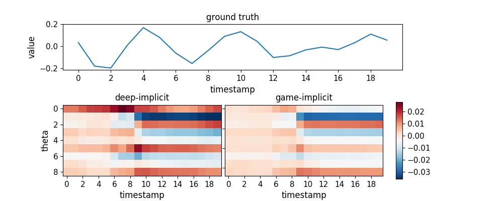
Figure 2: Visualization of weight vectors for predicting the first channel along each autoregressive timestamp in bearing dataset. The $y$-axis from $0$ to $8$ denotes $(\theta_{0})_{1}$, $(\theta_{1})_{1,1:4}$ and $(\theta_{2})_{1,1:4}$

.

We validate our approach on two real-world applications: a bearing dataset from NASA (Lee et al., 2016) and a stock market dataset consisting of historical data from the S&P 500 index. The bearing dataset records 4-channel acceleration data on 4 co-located bearings, and stock dataset records daily prices (4 channels in open, high, low, and close). Due to the diverse range of stock prices, we transform the data to daily percentage difference. We divide the sequence into disjoint subsequences and train the sequence generative model on them. The input and output length are decided based on the nature of dataset. The bearing dataset has a high frequency period of 5 points and low frequency period of 20 points. On the stock dataset, we used 1 month to predict the next week’s prices. The statistics of the processed dataset is shown in Table 1. We randomly sample $85\%$, $5\%$, and $10\%$ of the data for training, validation, and testing.

We set neighborhood $\epsilon$ and Markov order $K$ to be $6$ and $7$ to impose sequence-level coherence in stock dataset; and $9$ and $2$ for smooth variation in bearing dataset. We parametrize $\mu(\cdot)$ and $\Sigma(\cdot)$ jointly by stacking $1$ layer of CNN, LSTM, and $2$ fully connected layers. We use Ridge regression with default parameter in scikit-learn (Pedregosa et al., 2011) to implement the AR model. For efficiency, $10\%$ of the sequences are sampled for regularization in each batch.

We compare our asymmetric game-theoretic approach (‘game’) against the same model class without an explainer (‘deep’). We use ‘implicit’ label to distinguish predictors from those ‘explicitly’ written in an AR-like form. Evaluation involves three different types of errors: ‘Error’ is the root mean squared error (RMSE) between greedy autoregressive generation and the ground truth; ‘Deviation’ is RMSE between the model prediction $\mu(x_{1:i})$ and the explainer $g_{x_{1:i}}(x_{1:i})$, estimated also for ‘deep’ that is not guided by the explainer; and ‘TV’ is the average total variation of $[\hat{\theta},\hat{\theta}_{0}]$ over any two consecutive time points. For testing, the explainer is estimated based on a greedy autoregressive generative trajectory. TV for implicit models is based on the parameters of the explainer $g_{x_{t}}$. For explicit models, deviation RMSE is the sum of AR and constant deviations as in Eq. (7), thus not directly comparable to the implicit ‘Deviation’ based only on output differences.

The results are shown in Table 2. TV is not meaningful for implicit formulation in stock dataset due to the size of the neighborhood. The proposed game reduces the gap between deep learning model and AR model on deviation and TV, while retaining promising prediction accuracy.

We also show results of implicit setting on bearing dataset for different $\lambda$ in Table 3. The trends in increasing error and decreasing deviation and TV are quite monotonic with $\lambda$. When $\lambda=0.1$, the ‘game’ model is even more accurate than ‘deep’ model due to regularization effect of the game.

We visualize the explanations from implicit setting ($[\theta_{0},\theta]$ in explainer model) over autoregressive generative trajectories in Figure 2. The explanation from the ‘game’ model is more stable. Compared to the ground truth, different temporal pattern after the $9^{\text{th}}$ point is captured by the explanations.

5 Conclusion

We provide a novel game-theoretic approach to interpretable temporal modeling. The game articulates how the predictor accuracy can be traded off against locally agreeing with a simple axiomatically interpretable explainer. The work opens up many avenues for future work, from theoretical analysis of the co-operative games to estimation of interpretable unfolded trajectories through GANs.

References

- Al-Shedivat et al. (2017) Al-Shedivat, Maruan, Dubey, Avinava, and Xing, Eric P. Contextual explanation networks. arXiv preprint arXiv:1705.10301, 2017.
- Alvarez-Melis & Jaakkola (2017) Alvarez-Melis, David and Jaakkola, Tommi S. A causal framework for explaining the predictions of black-box sequence-to-sequence models. Proceedings of EMNLP, 2017.
- Arras et al. (2017) Arras, Leila, Horn, Franziska, Montavon, Grégoire, Müller, Klaus-Robert, and Samek, Wojciech. ” What is relevant in a text document?”: An interpretable machine learning approach. PloS one, 12(8):e0181142, 2017.
- Goodfellow et al. (2014) Goodfellow, Ian, Pouget-Abadie, Jean, Mirza, Mehdi, Xu, Bing, Warde-Farley, David, Ozair, Sherjil, Courville, Aaron, and Bengio, Yoshua. Generative adversarial nets. In Advances in neural information processing systems, pp. 2672–2680, 2014.
- Lakkaraju et al. (2016) Lakkaraju, Himabindu, Bach, Stephen H, and Leskovec, Jure. Interpretable decision sets: A joint framework for description and prediction. In Proceedings of the 22nd ACM SIGKDD International Conference on Knowledge Discovery and Data Mining, pp. 1675–1684. ACM, 2016.
- Lee et al. (2016) Lee, J., Qiu, H., Yu, G., Lin, J., and Rexnord Technical Services (2007). IMS, University of Cincinnati. Bearing data set. NASA Ames Prognostics Data Repository (http://ti.arc.nasa.gov/project/prognostic-data-repository), NASA Ames Research Center, Moffett Field, CA, 7(8), 2016.
- Lei et al. (2016) Lei, Tao, Barzilay, Regina, and Jaakkola, Tommi. Rationalizing Neural Predictions. In EMNLP 2016, Proceedings of the 2016 Conference on Empirical Methods in Natural Language Processing, pp. 107–117, 2016. URL http://arxiv.org/abs/1606.04155.
- Pedregosa et al. (2011) Pedregosa, F., Varoquaux, G., Gramfort, A., Michel, V., Thirion, B., Grisel, O., Blondel, M., Prettenhofer, P., Weiss, R., Dubourg, V., Vanderplas, J., Passos, A., Cournapeau, D., Brucher, M., Perrot, M., and Duchesnay, E. Scikit-learn: Machine learning in Python. Journal of Machine Learning Research, 12:2825–2830, 2011.
- Ribeiro et al. (2016) Ribeiro, Marco Tulio, Singh, Sameer, and Guestrin, Carlos. ”Why Should I Trust You?”: Explaining the Predictions of Any Classifier. In Proceedings of the 22Nd ACM SIGKDD International Conference on Knowledge Discovery and Data Mining, pp. 1135–1144, New York, NY, USA, 2016. ACM. ISBN 978-1-4503-4232-2. doi: 10.1145/2939672.2939778. URL http://arxiv.org/abs/1602.04938http://doi.acm.org/10.1145/2939672.2939778.
- Selvaraju et al. (2016) Selvaraju, Ramprasaath R, Cogswell, Michael, Das, Abhishek, Vedantam, Ramakrishna, Parikh, Devi, and Batra, Dhruv. Grad-cam: Visual explanations from deep networks via gradient-based localization. See https://arxiv. org/abs/1610.02391 v3, 7(8), 2016.
- Van Den Oord et al. (2016) Van Den Oord, Aaron, Dieleman, Sander, Zen, Heiga, Simonyan, Karen, Vinyals, Oriol, Graves, Alex, Kalchbrenner, Nal, Senior, Andrew, and Kavukcuoglu, Koray. Wavenet: A generative model for raw audio. arXiv preprint arXiv:1609.03499, 2016.
- Wu et al. (2018) Wu, Mike, Hughes, Michael C., Parbhoo, Sonali, Zazzi, Maurizio, Roth, Volker, and Doshi-Velez, Finale. Beyond sparsity: Tree regularization of deep models for interpretability. In Proceedings of the Thirty-Second AAAI Conference on Artificial Intelligence, New Orleans, Louisiana, USA, February 2-7, 2018, 2018. URL https://www.aaai.org/ocs/index.php/AAAI/AAAI18/paper/view/16285.