Quasi Markov Chain Monte Carlo Methods

Abstract

Quasi-Monte Carlo (QMC) methods for estimating integrals are attractive since the resulting estimators typically converge at a faster rate than pseudo-random Monte Carlo. However, they can be difficult to set up on arbitrary posterior densities within the Bayesian framework, in particular for inverse problems. We introduce a general parallel Markov chain Monte Carlo (MCMC) framework, for which we prove a law of large numbers and a central limit theorem. In that context, non-reversible transitions are investigated. We then extend this approach to the use of adaptive kernels and state conditions, under which ergodicity holds. As a further extension, an importance sampling estimator is derived, for which asymptotic unbiasedness is proven. We consider the use of completely uniformly distributed (CUD) numbers within the above mentioned algorithms, which leads to a general parallel quasi-MCMC (QMCMC) methodology. We prove consistency of the resulting estimators and demonstrate numerically that this approach scales close to $n^{-2}$ as we increase parallelisation, instead of the usual $n^{-1}$ that is typical of standard MCMC algorithms. In practical statistical models we observe multiple orders of magnitude improvement compared with pseudo-random methods.

1 Introduction

For many problems in science MCMC has become an indispensable tool due to its ability to sample from arbitrary probability distributions known up only to a constant. Comprehensive introductions on MCMC methods can be found in [NB99, Liu08, RC04, LB14]. Estimators resulting from MCMC scale independently of dimensionality. However, they have the fairly slow universal convergence rate of $n^{-1}$, where $n$ denotes the number of samples generated, in the mean squared error (MSE), same as classic Monte Carlo methods using pseudo-random numbers. For the latter, faster convergence rates of order close to $n^{-2}$ can be achieved when samples are generated by a suitable low-discrepancy sequence, i.e. points which are homogeneously distributed over space ([DKS13]). These so called quasi-Monte Carlo (QMC) methods, despite their generally deteriorating performance with increasing (effective) dimension ([WF03, CMO97]), can nonetheless lead to significant computational savings compared to standard Monte Carlo. However, they generally require the integral of interest to be expressible in terms of an expectation with respect to a unit hypercube, which limits their general application.

The first applications of QMC in the context of MCMC go back to [Che67] and [Sob74], which assume a discrete state space. In [Che67], the driving sequence of uniformly distributed independent and identically distributed (IID) random numbers is replaced by a completely uniformly distributed (CUD) sequence. The same approach is used in [OT05] and [CDO⁺11]. In [Lia98], a Gibbs sampler that runs on randomly shuffled QMC points is introduced. Later, [Cha04] uses a weighting of rejected samples to generate balanced proposals. Both successfully applied QMC in MCMC, albeit without providing any theoretical investigation. [CL07] uses QMC in multiple-try Metropolis-Hastings, and [LS06] within an exact sampling method introduced by [PW96]. In [LLT08] the so called array-randomised QMC (RQMC) was introduced that uses quasi-Monte Carlo to update multiple chains that run in parallel. Further, the roter-router model, which is a deterministic analogue to a random walk on a graph, was applied in [DF09] on a number of problems. We note that most of these approaches resulted in relatively modest performance improvements over non-QMC methods [CDO⁺11].

Based on the coupling argument by Chentsov from [Che67], it was proven in [OT05] that an MCMC method defined on a finite state space still has the correct target as its stationary distribution when the driving sequence of IID numbers is replaced by weakly CUD (WCUD) numbers. Subsequently, [TO08] provided proofs of some theoretical properties of WCUD sequences, along with numerical results using a Gibbs sampler driven by WCUD numbers, which achieves significant performance improvements compared to using IID inputs. More recently, the result from [OT05] was generalised to WCUD numbers and continuous state spaces by Chen ([CDO⁺11]).

In this work, we consider the theoretical and numerical properties of the parallel MCMC method introduced in [Cal14], which we here call multiple proposal MCMC (MP-MCMC) as it proposes and samples multiple points in each iteration. We extend this methodology to the use of non-reversible transition kernels and introduce an adaptive version, for which we show ergodicity. Further, we derive an importance sampling MP-MCMC approach, in which all proposed points from one iteration are accepted and then suitably weighted in order to consistently estimate integrals with respect to the posterior. We then combine these novel MP-MCMC algorithms with QMC by generalising them to use arbitrary CUD numbers as their driving sequence, and we establish conditions under which consistency holds. Due to the fact that the state space is covered by multiple proposals in each iteration, one might expect that using QMC numbers as the seed in MP-MCMC should harvest the benefits of low-discrepancy sequences more effectively than in the single proposal case previously considered. Moreover, the importance sampling approach mentioned above enables MP-MCMC to remove the discontinuity introduced by the acceptance threshold when sampling from the multiple proposals, which improves the performance when using QMC numbers as the driving sequence. Indeed, when combining the multiple proposal QMC approach together with the importance sampling method we observe in numerical simulations a convergence rate of order close to $n^{-2}$ for this novel MCMC method, similar to traditional QMC methods.

This work is, to the best of our knowledge, the first publication showing substantial benefits in the use of QMC in MCMC for arbitrary posteriors that are not known analytically and are not hierarchical, i.e. do not possess a lower-dimensional structure for their conditional probabilities. Hierarchical MCMC sampling problems using QMC for medium dimensions that have been considered in the literature include the $11$-dimensional hierarchical Poisson model for pump failures from [GS90], which was treated via QMC Gibbs sampling methods by [Lia98] and [OT05], respectively, and a $42$-dimensional probit regression example from [Fin47], treated in [TO08] via the use of a QMC seed in a Gibbs sampling scheme introduced in [AC93]. In these problems however, conditional distributions are available explicitly such that direct sampling can be applied.

In this paper, we begin with re-defining the MP-MCMC algorithm previously introduced in [Cal14] and then consider a number of novel extensions, which result finally in a parallel CUD driven method that achieves a higher rate of convergence similar to QMC. The list of novel algorithms we consider is presented in Table 1. Throughout the paper, we also prove some theoretical results for the proposed algorithms as well as investigating their performance in practice. For the purpose of clarity and readability, we will often state the lemma and refer the reader to the appropriate section in the appendix for its full proof.

Table 1: Summary of algorithms introduced in this work, and associated properties

Algorithm	Section	Adaptive	IS	PSR	CUD	Num. conv. rate
1	3.1	✗	✗	✓	✗	$n^{-1}$
2	3.7.3	✓	✗	✓	✗	$n^{-1}$
3	4.2	✗	✓	✓	✗	$n^{-1}$
4	4.2.2	✓	✓	✓	✗	$n^{-1}$
5	5.1.1	✗	✗	✗	✓	$n^{-1}$
6	5.2.1	✗	✓	✗	✓	$\approx n^{-2}$
7	5.3.1	✓	✓	✗	✓	$\approx n^{-2}$

In Section 2 we introduce the basics of QMC and give a short review of the literature regarding CUD points, discuss some CUD constructions and display the construction used in this work.

Next, in Section 3, we present the multiple proposal MCMC (MP-MCMC) framework from [Cal14], first using pseudo-random numbers, and introduce two new formulations of MP-MCMC as a single state Markov chain over a product space, which we use for proving a number of theoretical properties. We also formally prove a law of large numbers and central limit theorem for MP-MCMC and carefully consider a variety of novel extensions. In particular, we consider the use of optimised and non-reversible transitions, as well as adaptivity of the proposal kernel, for which we prove ergodicity. We then compare their relative performance through a simulation study.

In Section 4 we consider the use of importance sampling within an MP-MCMC framework. We suggest an adaptive version of this algorithm and prove its ergdocity, and consider the importance sampling approach as the limiting case of sampling from the finite state Markov chain on the multiple proposals. We conclude by proving asymptotic unbiasedness of the proposed methods and empirically comparing their performance.

In Section 5 we generalise the previously introduced MP-MCMC algorithms to the case of using CUD numbers as the driving sequence, instead of pseudo-random numbers. We describe two regularity conditions that we then use to prove consistency of the proposed method, and we discuss how CUD numbers should be best incorporated within MCMC algorithms generally. We prove asymptotic unbiasedness of the two proposed algorithms and demonstrate through a couple of numerical simulations an increased convergence rate of the empirical variance of our estimators, approaching $n^{-2}$ rather than usual $n^{-1}$ for traditional MCMC methods.

Finally, we present some conclusions and discuss the very many avenues for future work.

2 Some Concepts from Quasi Monte Carlo

Quasi-Monte Carlo (QMC) techniques approximate integrals by an equal-weight quadrature rule similar to standard Monte Carlo. However, instead of using IID random samples as evaluation points, one uses low-discrepancy sequences designed to cover the underlying domain more evenly. Common choices for such sequences for QMC include Sobol sequences and digital nets [DKS13]. Due to the increased spatial coverage of the domain QMC generally yields better convergence rates than standard Monte Carlo.

2.1 QMC background

Standard QMC approaches generally permit the use of a high-dimensional hypercube as the domain of integration. However, using standard approaches, e.g., inverse transformations as introduced in [Dev86], samples from arbitrary domains may be constructed, as long as the inverse CDF is available. When the inverse of the CDF is not available directly, one must resort to alternative sampling methods, which motivates the development of the MCMC methods later in this paper.

2.1.1 Discrepancy and Koksma-Hlawka inequality

Estimators based on QMC use a set of deterministic sample points $\bm{x}_{i}\in[0,1]^{d}$ for $i=1,...,n$ and $d\in\mathbb{N}$, that are members of a low-discrepancy sequence. Roughly speaking, these points are distributed inside $[0,1]^{d}$ such that the uncovered areas are minimised. Typically, the same holds true for projections of these points onto lower-dimensional faces of the underlying hypercube. Referring to [Nie92], for a set of QMC points $P=\{\bm{x}_{1},...,\bm{x}_{n}\}$, the star discrepancy can be defined as

$$D^{*d}_{n}(P)=\sup_{\bm{a}\in(0,1]^{d}}\left|\frac{1}{n}\sum_{i=1}^{n}\mathbf{I}_{(0,\bm{a}]}(\bm{x}_{i})-\prod_{i=1}^{n}a_{i}\right|,$$ (1)

where $\bm{a}$ has coordinates $0\leq a_{j}\leq 1$ for any $j=1,...,d$, respectively. This gives us a measure of how well-spaced out a set of points is on a given domain. One of the main results in QMC theory, the Koksma-Hlawka inequality, provides an upper bound for the error of a QMC estimate based on (1) by

$$\left|\frac{1}{n}\sum_{i=1}^{n}f(\bm{x}_{i})-\int_{[0,1]^{d}}f(\bm{x})\mathrm{d}\bm{x}\right|\leq V\left(f\right)\cdot D^{*d}_{n}(P),$$ (2)

where $V(f)$ denotes the variation of $f$ in the sense of Hardy-Krause. For a sufficiently smooth $f$, $V(f)$ can be expressed as the sum of terms

$$\int_{[0,1]^{k}}\left|\frac{\partial^{k}f}{\partial x_{i_{1}}...\partial x_{i_{k}}}\right|_{x_{j}=1,j\neq i_{1},...,i_{k}}\mathrm{d}x_{i_{1}}...\mathrm{d}x_{i_{k}},$$ (3)

where $i_{1}<...<i_{k}$ and $k\leq d$. A more general definition for the case of non-smooth $f$ and in a multi-dimensional setting is beyond the scope of this work, but can be found in [Owe05]. In (2), $V(f)$ is assumed to be finite. Thus, the error of the approximation is deterministically bounded by a smoothness measure of the integrand and a quality measure for the point set. The Koksma-Hlawka equation (2) (for the case $d=1$) was first proven by Koksma [Kok42], and the general case ($d\in\mathbb{N}$) was subsequently proven by Hlawka [Hla61]. Note that for some functions arising in practise it holds $V(f)=\infty$, e.g. the inverse Gaussian map from the hypercube to the hypersphere [BO16], so that equation (2) cannot be applied.

2.1.2 Convergence rates

The use of low-discrepancy sequences instead of pseudorandom numbers may allow a faster convergence rate of the sampling error. Given an integrand $f$ with $V(f)<\infty$, constructions for QMC points can achieve convergence rates close to $\mathcal{O}(n^{-2})$ in the MSE, compared to $\mathcal{O}(n^{-1})$ for standard Monte Carlo [DKS13]. For smooth functions, it is possible to achieve convergence rates of order $\mathcal{O}(n^{-2\alpha}\log(n)^{2d\alpha})$ when $f$ is $\alpha$-times differentiable ([Dic09]). However, if $f$ has only bounded variation but is not differentiable, convergence rates of in general only $\mathcal{O}(n^{-2}\log(n)^{2d})$ hold true [Sha63]. For practical applications where the dimensionality $d$ is large and the number of samples $n$ is moderate, QMC does therefore not necessarily perform better than standard Monte Carlo. In some settings, using randomised QMC (RQMC) one can achieve convergence rates of $\mathcal{O}(n^{-3})$ [LLT06, LLT08] in MSE, and $n^{-3}$ for the empirical variance in certain examples [LMLT18].

2.1.3 The curse of dimensionality

The curse of dimensionality describes the phenomenon of exceeding increase in the complexity of a problem with the dimensionality it is set in [Ric57]. Classical numerical integration methods such as quadrature rules become quickly computationally infeasible to use when the number of dimensions increases. This is since the number of evaluation points typically increases exponentially with the the dimension, making such integration schemes impractical for dimensions that are higher than say $d=6$. However, in [PT⁺95] a high-dimensional ($d=360$) problem from mathematical finance was successfully solved using quasi-Monte Carlo (Halton and Sobol sequences). Since then, much research has been undertaken to lift the curse of dimensionality in QMC, referring to [KS05], [DP10] and [DKS13].

In general, a well-performing integration rule in a high-dimensional setting will depend on the underlying integrand or a class of integrands. [CMO97] introduced the notion of effective dimension, which identifies the number of coordinates of a function or indeed of a suitable decomposition (e.g. ANOVA), respectively, which carries most of the information about the function. This concept accounts for the fact that not all variables in a function are necessarily informative about the variability in the function, and may therefore be neglected when integrated. In practical applications the effective dimension can be very low ($d=2,3$) compared to the actual number of variables in the integrand. To model such situations, weighted function spaces have been introduced in [SW98]. In principle, the idea is to assign a weight to every coordinate or to any subset of coordinates for a particular decomposition of the integrand, thereby prioritising variables with high degree of information on the integrand. Weighted function spaces have a Hilbert space structure. For a particular class of such spaces, namely reproducing kernel Hilbert spaces (RKHS), the worst-case error of the integration, defined as the largest error for any function in the unit ball of the RKHS, can be expressed explicitely in terms of the reproducing kernel. Based on this, it is possible to prove the existence of low-discrepancy sets that provide an upper bound of the worst-case error proportional to $N^{-1+\delta}$ for any $\delta>0$, where the constant does neither depend on $N$ nor on $d$. Furthermore, there exist explicit constructions for such amenable point sets, e.g. the greedy algorithm for shifted rank-1 lattice rules by [SKJ02] and the refined fast implementation based on Fast Fourier Transforms provided by [NC06]. Modern quasi-Monte Carlo implementations can thus be useful in applications with up to hundreds and even thousands of dimensions.

The constructions of QMC point sets used for MCMC in this work are generic in the sense that their construction does actually not depend on the underlying integrand. Major performance gains compared to standard Monte Carlo can still be achieved for moderately large dimensions, which we will see in Section 5. However, the incorporation of QMC constructions tailored to an inference problem solved by MCMC could a valuable future extension of this work.

2.1.4 Randomised QMC

Despite possibly far better convergence rates of QMC methods compared to standard MCMC, they produce estimators that are biased and lack practical error estimates. The latter is due to the fact that evaluating the Koksma-Hlawka inequality requires not only computing the star discrepancy, which is an NP-hard problem [GSW09], but also computing the total variation $V(f)$, which is generally even more difficult than integrating $f$. However, both drawbacks can be overcome by introducing a randomisation into the QMC construction which preserves the underlying properties of the QMC point distribution. For this task, there have been many approaches suggested in the literature, such as shifting using Cranley-Patterson rotations [CP76], digital shifting [DKS13], and scrambling [Owe97, O⁺97]. In some cases, randomisation can even improve the convergence rate of the unrandomised QMC method, e.g. scrambling applied to digital nets in [O⁺97, Dic11] under sufficient smoothness conditions. In these situations, the average of multiple QMC randomisations yields a lower error than the worst-case QMC error.

2.1.5 Completely uniformly distributed points

Conceptually, QMC is based on sets of points which fill an underlying hypercube homogeneously. Through suitable transformations applied to those points, samples are created which respresent the underlying target. In constrast, MCMC relies on an iterative mechanism which makes use of ergodicity. More presicely, based on a current state a subsequent state is proposed and then accepted or rejected, in such a way that the resulting samples represent the underlying target. In that sense, QMC is about filling space, relying on equidistributedness, while MCMC is about moving forward in time, relying on ergodicity. Averages of samples can therefore be considered as space averages in QMC and time-averages in MCMC, respectively.

Standard MCMC works in the following way: based on a given $d$-dimensional sample, a new sample is proposed using $d$ IID random numbers in $(0,1)$ using a suitable transformation. Then an accept/reject mechanism is employed, i.e. the proposed sample is accepted with a certain probability, for which another random point in $(0,1)$ is required. Thus, for $n$ steps we require $n(d+1)$ points, $u_{1},...,u_{n(d+1)}\in(0,1)$. The idea in applying QMC to MCMC is to replace the IID points $u_{i}$, for $i=1,...,n(d+1)$, by more evenly distributed points. There are two sources for problems connected to this approach: first, the sequence of states in the resulting process will not be Markovian, and thus consistency is not straightforward as the standard theory relies on the Markovian assumption. However, we know for instance from adaptive MCMC that even if the underlying method is non-Markovian ergodicity can still be proven [HST⁺01, HLMS06, RR07, ŁRR13, AM⁺06, RR09, AT08].

Typically, computer simulations of MCMC are driven by a pseudo-random number generator (PRNG). A PRNG is an algorithm that generates a sequence of numbers which imitate the properties of random numbers. The generation procedure is however deterministic as it is entirely determined by an initial value. We remark that carefully considered, a sequence constructed by an MCMC method using a PRNG does therefore actually not fulfill the Markov property either since the underlying seed is deterministic. However, it is generally argued that given a good choice, a pseudo-random number sequence has properties that are sufficiently similar to actual IID numbers as to consider the resulting algorithm as probabilistic. A first formal criteria for a good choice of pseudo-random numbers typically used in computer simulations was formulated in Yao’s test [Yao82]. Roughly speaking, a sequence of words passes the test if, given a reasonable computational power, one is not able to distinguish from a sequence generated at random. For modern versions of empirical tests for randomness properties in PRNGs we refer to the Dieharder test suite [BEB17] and the Test01 software library [LS07]. As an example, the spacings of points which are selected according to the underlying PRNG on a large interval are tested for being exponentially distributed. Asymptotically, this holds true for the spacings of truly randomly chosen points.

A second source of problems in using QMC seeds in MCMC arises since MCMC is inherently sequential, which is a feature that QMC methods generally do not respect. For example, the Van der Corput sequence ([VdC35]), which will be introduced below, has been applied as a seed for MCMC in [MC93]. In their example, the first of an even number of heat particles, which are supposed to move according to a symmetric random walk, always moves to the left, when sampled by the Van der Corput sequence. This peculiar behaviour occurs since, although the VdC-sequence is equidistristributed over $[0,1]$, non-overlapping tupels of size $d=2m$ for $m\in\mathbb{N}$ are not equidistributed over $[0,1]^{d}$, as is shown later.

The convergence of a QMC method, i.e. the succesful integration of a function on $\mathbb{R}^{d}$, relies on the equidistributedness of tupels $(u_{(n-1)d+1},...,u_{nd})\in[0,1]^{d}$ for $n\rightarrow\infty$, where $d$ is fixed. In order to prevent failure when using QMC in MCMC such as in [MC93], tupels of the form $(u_{(n-1)d^{\prime}+1},...,u_{nd^{\prime}})\in[0,1]^{d^{\prime}}$ must satisfy equidistributedness for $n\rightarrow\infty$ while $d^{\prime}$ is variable. This naturally leads us to the definition of CUD numbers: a sequence $(u_{i})_{i}\subset[0,1]$ is called completely uniformly distributed (CUD) if for any $d\geq 1$ the points $\bm{x}^{(d)}_{i}=(u_{i},\ldots,u_{i+d-1})\in[0,1]^{d}$ fulfill

$$D_{n}^{*d}(\bm{x}_{1}^{(d)},\ldots,\bm{x}_{n}^{(d)})\rightarrow 0,\quad\text{ as }\quad n\rightarrow\infty.$$

In other words, any sequence of overlapping blocks of $u_{i}$ of size $d$ yield the desirable uniformity property $D_{n}^{*d}\rightarrow 0$ for a CUD sequence $(u_{i})_{i\geq 1}$. It was shown in [Che67] that this is equivalent to any sequence of non-overlapping blocks of $u_{i}$ of size $d$ satisfying $D_{n}^{*d}\rightarrow 0$, i.e.

$$D_{n}^{*d}(\bm{\tilde{x}}_{1}^{(d)},\ldots,\bm{\tilde{x}}_{n}^{(d)})\rightarrow 0,\quad\text{ as }\quad n\rightarrow\infty,$$ (4)

where $\bm{\tilde{x}}_{i}^{(d)}:=(u_{d(i-1)+1},\ldots,u_{di})\in[0,1]^{d}$. In [CDO⁺11], Chen et al. prove that if in standard MCMC the underlying driving sequence of IID numbers is replaced by CUD numbers, the resulting algorithm consistently samples from the target distribution under certain regularity conditions. One can easily show that every sequence of IID numbers is also CUD.

Constructions in the literature

There are a number of techniques to construct CUD sequences in the literature. In [Lev99], several constructions of CUD sequences are introduced, but none of them amenable for actual implementation [Che11]. In [Che11], an equidistributed linear feedback shift register (LFSR) sequence implemented by Matsumoto and Nishimura is used, which is shown to have the CUD property. In [OT05] the author uses a CUD sequence that is based on the linear congruential generator (LCG) developed in [EHL98]. The lattice construction from [Nie77] and the shuffling strategy for QMC points from [Lia98] are also both shown to produce CUD points in [TO08]. Furthermore, [CMNO12] presents constructions of CUD points based on fully equidistributed LFSR, and antithetic and round trip sampling, of which the former we will use for our simulations later on. The construction introduced in [TO08] relies on a LCG with initial seed $1$ and increment equal to zero. For a given sequence length, a good multiplier is found by the primitive roots values displayed in [Lec99].

Illustration of a CUD sequence

As an illustration, we display in Figure 1 an implementation of the the CUD construction, which was introduced in [CMNO12] and relies on a LFSR with a transition mechanism based on primitive polynomials over the Galois field $GF(2)$. The resulting sequence is visually more homogeneously distributed than that generated using pseudo-random numbers. For a complete description of the construction, sufficient for a reader to implement the method themselves, we refer to section 3 in [CMNO12]. Additionally, we provide our own Python implementation of this CUD generator in [Sch18], as well as the one introduced by [TO08].

Construction used in this work

Given a target defined on a $d$-dimensional space we employ a technique of running through a generated CUD sequence $d$ times, similar to [OT05], thereby creating tupels of size $d$. The resulting tupels are pairwise different from each other and every tupel is used exactly once in the simulation. Similarly to [OT05], we prepend a tupel of values close to zero to the resulting tupel sequence, imitating the property of an integration lattice containing a point at the origin.
More precisely, we use the CUD construction based on section 3 in [CMNO12], which creates sequences of length $L=2^{m}-1$ for integers $10\leq m\leq 32$. Given a sequence $u_{1},...,u_{L}\in(0,1)$ and dimensionality $d$, we cut off the sequence at $T:=\lfloor L/d\rfloor\cdot d\leq L$, leading to the trimmed sequence $u_{1},...,u_{T}$. Since $L-T\leq d\ll T,L$, trimming has no relevant influence on the outcomes of simulations. In order to make efficient use of the generated sequence, we generate tupels of size $d$ and of the form

$$(u_{1},...,u_{d}),(u_{d+1},\ldots,u_{2d}),...,(u_{T-d+1},...,u_{T}),$$

$$(u_{2},...,u_{d+1}),(u_{d+2},\ldots,u_{2d+1}),...,(u_{T-d+2},...,u_{T},u_{1}),$$

$$...$$

$$(u_{d},...,u_{2d-1}),(u_{2d},\ldots,u_{3d-1}),...,(u_{T},u_{1},...,u_{d-1}).$$

The sequence of points $v_{n}$, $n=1,...,dT$, given by $u_{1},...,u_{T}$, $u_{2},...,u_{T},u_{1}$, $...$, $u_{d},...,u_{T},u_{1},...,u_{d-1}$, still satisfies the CUD property. This is true since the shifting of indices in $u_{1},...,u_{T}$ to $u_{k+1},...,u_{T},u_{1},...,u_{k}$ for any $k\in\mathbb{N}$ does not influence the CUD property. Further, appending a CUD sequence to another CUD sequence of the same length preserves the CUD property, too. Finally, prepending a single tupel of size $d$ does not affect the CUD property for overlapping tupels of size $d$.

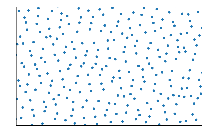
(a) A completely uniformly distributed sequence.

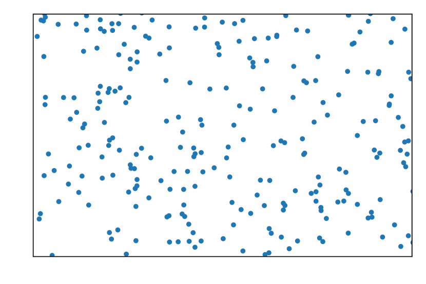
(b) A pseudo-randomly generated sequence.

Figure 1: Segments of CUD and pseudo-random finite sequences in $(0,1)^{2}$.

QMC sequences are generally not CUD

Finally we note that care must be taken in the choice of the QMC sequence applied to MCMC since not every low discrepancy sequence is a CUD sequence. For the van der Corput sequence $(u_{n})_{n}$ ([VdC35]), any $u_{2n}\in(0,1/2)$ and any $u_{2n-1}\in[1/2,1)$ for all $n\geq 1$. Thus,

$$\bm{x}^{(2)}_{2n} \in(0,1/2)\times[1/2,1),\text{ and }$$ (5)

$$\bm{x}^{(2)}_{2n-1} \in[1/2,1)\times(0,1/2).$$ (6)

Therefore, the sequence of overlapping tupels $\bm{x}^{(2)}_{n}$ never hits the square $(0,1/2)\times(0,1/2)$, which implies $D^{*2}_{n}\geq 1/4$ for any $n$. Note that the same holds true for non-overlapping tupels $\tilde{\bm{x}}^{(2)}_{n}$. Hence, the van der Corput sequence is not a CUD sequence.

3 Pseudo-random MP-MCMC

In [Cal14], a natural generalisation of the well-known Metropolis-Hastings algorithm ([Has70]) that allows for parallelising a single chain is achieved by proposing multiple points in parallel. In every MCMC iteration, samples are drawn from a finite state Markov chain on the proposed points, which is constructed in such a way that the overall procedure has the correct target density $\pi$ on a state space $\Omega\subset\mathbb{R}^{d}$ for $d\in\mathbb{N}$, as its stationary distribution. In this section we introduce this algorithm, demonstrate that this approach mathematically corresponds to a Metropolis-Hastings algorithm over a product space and prove its consistency, as well as some asymptotic limit theorems, before considering how to extend this algorithm to improve its sampling performance.

3.1 Derivation

Before presenting the MP-MCMC algorithm we first note that any joint probability distribution $p(\bm{y}_{1:N+1})$, where $\bm{y}_{1:N+1}=\bm{y}_{[1:N+1]}=(\bm{y}_{1},...,\bm{y}_{N+1})$ with $\bm{y}_{i}\in\Omega$ $\forall i=1,...,N+1$, can be factorised in $N+1$ different ways, using conditional probabilities of the form, $p(\bm{y}_{1:N+1})=p(\bm{y}_{i})p(\bm{y}_{\setminus i}|\bm{y}_{i})$, where $\bm{y}_{\setminus i}:=\bm{y}_{[1:i-1,i+1:N+1]}$. If the target $\pi$ is the marginal distribution for $\bm{y}_{i}$ of $\bm{y}_{1:N+1}\sim p$ and any $i=1,...,N+1$, then

$$p(\bm{y}_{1:N+1})=\pi(\bm{y}_{i})\kappa(\bm{y}_{i},\bm{y}_{\setminus i}),$$

for a proposal distribution $\kappa$ satisfying $\kappa(\bm{y}_{i},\bm{y}_{\setminus i})\equiv p(\bm{y}_{\setminus i}|\bm{y}_{i})$. Thus, in the $i$th factorisation, $\bm{y}_{i}\sim\pi$, while the other $\bm{y}_{\setminus i}\sim\kappa(y_{i},\cdot)$ Referring to [Tje04, Cal14], a uniform auxiliary variable $I\in\{1,...,N+1\}$ can be introduced that determines which factorisation is used, such that

$$p(\bm{y}_{1:N+1},I=i)=\frac{1}{N+1}\pi(\bm{y}_{i})\kappa(\bm{y}_{i},\bm{y}_{\setminus i}).$$ (7)

Input: Initialise starting point $\bm{x}_{0}=\bm{y}_{1}\in\Omega\subset\mathbb{R}^{d}$, number of proposals $N$, number of accepted samples per iteration $M$, auxiliary variable $I=1$ and counter $n=1$;

1 for each MCMC iteration $\ell=1,2,...$ do

2       Sample $\bm{y}_{\setminus I}$ conditioned on $I$, i.e., draw $N$ new points from the proposal kernel $\kappa(\bm{y}_{I},\cdot)=p(\bm{y}_{\setminus I}|\bm{y}_{I})$ ;

3       Calculate the stationary distribution of $I$ conditioned on $\bm{y}_{1:N+1}$, i.e. $\forall$ $i=1,...,N+1$, $p(I=i|\bm{y}_{1:N+1})=\pi(\bm{y}_{i})\kappa(\bm{y}_{{i}},\bm{y}_{\setminus{i}})/\sum_{j}\pi(\bm{y}_{j})\kappa(\bm{y}_{{j}},\bm{y}_{\setminus{j}})$, which can be done in parallel;

4       for $m=1,...,M$ do

5             Sample new $I$ via the stationary distribution $p(\cdot|\bm{y}_{1:N+1})$;

6             Set new sample $\bm{x}_{n+m}=\bm{y}_{I}$;

7            

8       end for

9      Update counter $n=n+M$

10 end for

Algorithm 1 Multiple-proposal Metropolis-Hastings

3.1.1 A Markov chain over a product space

The MP-MCMC method generates $M\in\mathbb{N}$ new samples per iteration, and can be considered as a single Markov chain over the product space of proposal and auxiliary variables $(\bm{y}_{1:N+1},I_{1:M})\in\Omega^{N+1}\times\{1,...,N+1\}^{M}$ by applying a combination of two transition kernels, each of which preserves the underlying joint stationary distribution. First, the states of a finite state Markov chain are created by updating the proposals $\bm{y}_{\setminus{i}}$ conditioned on $\bm{y}_{i}$ and $I_{M}=i$, which clearly preserves the joint target distribution as we sample directly from $\kappa(\bm{y}_{i},\cdot)$; this is equivalent to a Gibbs sampling step. The choice of the proposal kernel is up to the practitioner, and kernels based on Langevin diffusion and Hamiltonian dynamics have successfully been applied ([Cal14]). Secondly, $I_{m}$ conditioned on $\bm{y}_{1:N+1}$ and $I_{m-1}$ is sampled $M$ times, i.e. for $m=1,...,M$, using a transition matrix $A$, where $A(i,j)=A(i,j|\bm{y}_{1:N+1})$ denotes the probability of transitioning from $I_{m-1}=i$ to $I_{m}=j$. Here, $I_{0}$ denotes the $M$th (i.e. last) sample of $I$, i.e. $I_{M}$, from the previous iteration. An illustration of this procedure is given in Figure 2. Using the factorisation from (7), the joint distribution of $(\bm{y}_{1:N+1},i_{m})$ for $I_{m}=i_{m}$ denoting the $m$th sample of $I$ and $m=1,...,M$, can be expressed as,

$$p(\bm{y}_{1:N+1},I_{m}=i_{m})=\frac{1}{N+1}\pi(\bm{y}_{i_{m}})\kappa(\bm{y}_{i_{m}},\bm{y}_{\setminus{i_{m}}}).$$

Observe that $\bm{y}_{i_{m}}$ has the correct density $\pi(\bm{y}_{i_{m}})$ for any $m=1,...,M$. Thus, those are the samples we collect in every iteration. For the particular case where $A(i,j)=p(I=j|\bm{y}_{1:N+1})$, independent of $i$, denotes the stationary transition matrix on the states $I_{1},...,I_{M}$ given $y_{1:N+1}$, the entire procedure described here is given in Algorithm 1. Note that, for the sake of clarity, we make a distinction between proposals $\bm{y}_{1:N+1}$ from one iteration, and the accepted samples $\bm{x}_{n}$ with $n\in\mathbb{N}$.

Figure 2: Visualisation of MP-MCMC as a single Markov chain on the product space of proposal samples and auxiliary variables

Considering MP-MCMC as a Markov chain over the product space of proposals and auxiliary variables has the advantage that a formula for the transition kernel of the resulting chain can be derived. This is useful for later statements considering ergodicity of adaptive versions of MP-MCMC in Section 3.7, which require computations on the transition probabilities.

3.1.2 Transition probabilities on the product space

An explicit form for the transition kernel density $\hat{P}(\tilde{z},z)$, from state $\tilde{z}=(\tilde{\bm{y}}_{1:N+1},\tilde{i}_{1:M})$ to state $z=(\bm{y}_{1:N+1},i_{1:M})$, where $\tilde{z},z\in\Omega^{N+1}\times\{1,...,N+1\}^{M}$, is given by,

$$\hat{P}(\tilde{z},z)=\kappa(\bm{y}_{i_{0}},\bm{y}_{\setminus{i_{0}}})\prod_{m=1}^{M}A(i_{m-1},{i_{m}})$$ (8)

where we implicitly used that $i_{0}=\tilde{i}_{M}$ and $\bm{y}_{i_{0}}=\tilde{\bm{y}}_{\tilde{i}_{M}}$. Waiving the latter assumption, we need to add the term $\delta_{\tilde{\bm{y}}_{\tilde{i}_{M}}}(\bm{y}_{i_{0}})$ to the expression of the transition kernel. A more thorough derivation of equation (8), as well as the subsequent equation (9), is presented in Appendix A.1. Let us introduce the notation $B_{1:{n}}=B_{1}\times...\times B_{n}$ for any sets $B_{1},...,B_{n}$ and $n\in\mathbb{N}$. Let $B\in\mathcal{B}(\Omega^{N+1})\times\mathcal{P}(\{1,...,N+1\}^{M})$ such that $B=C_{1:{N+1}}\times D_{1:M}\subset\Omega^{N+1}\times\{1,...,N+1\}^{M}$, where $\mathcal{P}(\{1,...,N+1\}^{M})$ denotes the power set of $\{1,...,N+1\}^{M}$. The probability $\operatorname{Pr}(z\in B|\tilde{z})=\hat{P}(\tilde{z},B)$ of a new state $z=(\bm{y}_{1:N+1},i_{1:M})\in B$ given a current state $\tilde{z}=(\tilde{\bm{y}}_{1:N+1},\tilde{i}_{1:M})$ with $\tilde{i}_{M}=i_{0}$ can be expressed as,

$$\hat{P}(\tilde{z},B)=\chi_{C_{i_{0}}(\tilde{\bm{y}}_{\tilde{i}_{M}})}\int_{C_{\setminus{i_{0}}}}\kappa(\bm{y}_{i_{0}}=\tilde{\bm{y}}_{\tilde{i}_{M}},\bm{y}_{\setminus{i_{0}}})\sum_{i_{1:M}\in D_{1:M}}\prod_{m=1}^{M}A(i_{m-1},i_{m}|\bm{y}_{i_{0}}=\tilde{\bm{y}}_{\tilde{i}_{M}})\mathrm{d}\bm{y}_{\setminus{i_{0}}},$$ (9)

where we use the notation $B_{\setminus{i}}=B_{1}\times...\times B_{i-1}\times B_{i+1}\times..\times B_{n}$ for any sets $B_{1},...,B_{n}$ and $i=1,...,n\in\mathbb{N}$. Note that conditioning on $\tilde{z}$ in (9) reduces to conditioning on the last accepted sample $\tilde{\bm{y}}_{\tilde{i}_{M}}$, which is the only sample of relevance for the subsequent iteration. Thus, the domain of the transition kernel $P$ can be reduced to $\Omega$ by using the identification $\hat{P}(\tilde{\bm{y}}_{\tilde{i}_{M}},B)\equiv\hat{P}(\tilde{z},B)$.

3.1.3 Equivalence of MP-MCMC to a chain on the accepted samples

An alternative representation of MP-MCMC as a Markov chain over the product space of proposals and auxiliary variables $(\bm{y}_{1:N+1},I_{1:M})$ in one iteration is to understand it as a chain over the space of accepted samples $(\bm{x}_{1},...,\bm{x}_{M})$ in one iteration. Indeed, given the current accepted set of samples, any set of samples generated in a future iteration are independent of the past iterations. This representation is useful since it allows to see MP-MCMC as a Markov chain over a single real space, which will be used to prove limit theorems in Section 3.6. Further, explicit transition probabilities for this representation are derived in what follows, which are then used to prove ergodicity statements of adaptive versions of MP-MCMC in Section 3.7. Note that since $\bm{x}_{i}\in\Omega$ for any $i=1,...,M$, we have $(\bm{x}_{1},...,\bm{x}_{M})\in\Omega^{M}$.

3.1.4 Transition probabilities on the accepted samples

Clearly, we would like to have an expression for the transitions between actual accepted states rather than proposal and auxiliary variables. It is possible to derive from the transition kernel $\hat{P}$, corresponding to the states of proposals and auxiliary variables $(\bm{y}_{1:N+1},I_{1:M})$, the transition kernel $P$, corresponding to only the actually accepted states $\bm{x}_{1:M}\in\Omega^{M}$, i.e. where $\bm{x}_{m}=\bm{y}_{I_{m}}$ for $m=1,...,M$. The probability of accepted states $\bm{x}_{1:M}\in B=B_{1:M}\in\mathcal{B}({\Omega^{M}})$ given a previous state $\tilde{\bm{x}}_{1:M}$ can be expressed in terms of the transition kernel $\tilde{P}$ on the model state space of proposals and auxiliary variables from (9) as follows,

$${P}(\tilde{\bm{x}}_{1:M},B) =\hat{P}\left(\tilde{\bm{x}}_{M},\bigcup_{i_{1},...,i_{M}=1}^{N+1}\ \bigcap_{m=1}^{M}S_{i_{m}}(B)\right)$$ (10)

where

$$S_{i_{m}}(B)=\Omega^{d(i_{m}-1)}\times B_{m}\times\Omega^{d(N+1-i_{m})}\times\{1:N+1\}^{m-1}\times\{i_{m}\}\times\{1:N+1\}^{M-m}$$ (11)

for any $i_{m}=1,...,N+1$ and $m=1,...,M$. The sets $S_{i_{m}}(B)$ are pairwise disjoint. A comprehensive derivation of equation (10) can be found in Appendix A.2.

3.2 Consistency

The question then arises how to choose the transition probabilities $A(i,j)$, for any $i,j=1,...,N+1$, such that the target distribution $\pi$ for accepted samples is preserved. Given the transition matrix $[A(i,j)]_{i,j}$ on the finite states $i,j$ determining the transitions of $I$, and using the factorisation in (7), the detailed balance condition for updating $I$ in $(\bm{y}_{1:N+1},I)$ is given by

$$\frac{1}{N+1}\pi(\bm{y}_{i})\kappa(\bm{y}_{i},\bm{y}_{\setminus{i}})A(i,j)=\frac{1}{N+1}\pi(\bm{y}_{i})\kappa(\bm{y}_{i},\bm{y}_{\setminus{i}})A(j,i),$$

for all $i,j=1,...,N+1$. Clearly, the detailed balance condition implies the balance condition,

$$\frac{1}{N+1}\pi(\bm{y}_{i})\kappa(\bm{y}_{i},\bm{y}_{\setminus{i}})=\sum_{j=1}^{N+1}\pi(\bm{y}_{j})\kappa(\bm{y}_{j},\bm{y}_{\setminus{j}})A(j,i),$$ (12)

for any $i=1,...,N+1$. If (12) holds true, the joint distribution $p(\bm{y}_{1:N+1},I)$ is invariant if $I$ is sampled using the transition matrix $A$. We say that the sequence $(\bm{x}_{i})_{i}$ of an MP-MCMC algorithm consistently samples $\pi$, if

$$\lim_{n\rightarrow\infty}\frac{1}{n}\sum_{i=1}^{n}f(\bm{x}_{i})=\int_{\Omega}f(\bm{x})\pi(\bm{x})\mathrm{d}\bm{x},$$ (13)

for any continuous bounded $f$ on $\Omega\subset\mathbb{R}^{d}$. We have chosen this notion of consistency to represent the fact that implicitely the formulation of low-discprenacy sets is closely related to the Riemannian integral, whose well-definedness is ensured for continuous and bounded functions. For further details we refer to the integrability condition introduced in Section 3.2. If the underlying Markov chain on the states $(\bm{y}_{1:N+1},I)$ satisfies (12) and is positive Harris with invariant distribution $p(\bm{y}_{1:N+1},I)$, then (13) holds true, which is an immediate consequence of the ergodic theorem, Theorem 17.1.7, in [MT12]. For a definition of positive Harris we refer to Section 10.1.1 in [MT12].

3.2.1 Sampling from the stationary distribution of $I$

As stated in Algorithm 1, one can sample directly from the steady-state distribution of the Markov chain, conditioned on $\bm{y}_{1:N+1}$. The stationary distribution of $I$, given $\bm{y}_{1:N+1}$, also used in [Cal14], equals

$$p(I=j|\bm{y}_{1:N+1})=\frac{\pi(\bm{y}_{j})\kappa(\bm{y}_{j},\bm{y}_{\setminus j})}{\sum_{k=1}^{N+1}\pi(\bm{y}_{k})\kappa(\bm{y}_{k},\bm{y}_{\setminus k})},$$ (14)

for any $j=1,...,N+1$. One can easily see that detailed balance holds for the stationary transition matrix $A(i,j)=p(I=j|\bm{y}_{1:N+1})$. Note that (14) is a generalisation of Barker’s algorithm [Bar65] for multiple proposals in one iteration. For $N=1$, the term on the right hand side reduces to Barker’s acceptance probability. Since this probability is always smaller or equal to Peskun’s acceptance probability, which is used in the usual Metropolis-Hastings algorithm, samples generated by Barker’s algorithm yield mean estimates with an asymptotic variance that is at least as large as when generated by Metropolis-Hastings [Pes73][Theorem 2.2.1]. A generalisation for Peskun’s acceptance probability in the multiple proposal setting is introduced in [Tje04], which aims to minimise the diagonal entries of the transition matrix iteratively starting from the stationary transition matrix, while preserving its reversibility. The resulting MP-MCMC method is investigated numerically in 3.5.

3.2.2 Sampling from the transient distribution of $I$

Instead of sampling $I$ from the stationary finite state Markov chain conditioned on $\bm{y}_{1:N+1}$, [Cal14] proposes the choice $A(i,j)=A(i,j|\bm{y}_{1:N+1})$, defined by

$$A(i,j)=\begin{cases}\frac{1}{N}\min(1,R(i,j))&\mbox{if }j\neq i\\ 1-\sum_{j\neq i}A(i,j)&\mbox{otherwise,}\end{cases}$$ (15)

where $R(i,j)={\pi(\bm{y}_{j})\kappa(\bm{y}_{j},\bm{y}_{\setminus j})}/{[\pi(\bm{y}_{i})\kappa(\bm{y}_{i},\bm{y}_{\setminus i})]}$. Referring to Proposition 1 in [Cal14], detailed balance is fulfilled for $A$ as given in (15). Note that this choice is a generalisation of the original Metropolis-Hastings acceptance probability. For $N=1$, i.e. if only a single state is proposed and a single state is accepted in each iteration, and if we replace the choice of $A$ in Algorithm 1 by (15), the resulting algorithm reduces to the usual Metropolis-Hastings algorithm.

3.3 Some practical aspects

In this section, we discuss some practical considerations regarding the use of MP-MCMC and some properties unique to this approach.

3.3.1 Parallelisation

In recent years, much effort has been focused on developing parallelisable MCMC strategies for performing inference on increasingly more computationally challenging problems. A number of specific approaches have been considered previously that incorporate different levels of parallelisation, for example subsampling data to scale MCMC algorithms to big data scenarios ([NWX13], [WD13]), parallelising geometric calculations used in designing efficient proposal mechanisms [WT11] and [AKW12], and for certain cases, parallelising the likelihood computation ([AD11], [SN10]).

One major advantage of MP-MCMC compared to many MCMC methods, including standard Metropolis-Hastings and other single proposal algorithms, is that it is inherently parallelisable as a single chain. More precisely, the likelihoods associated with the multiple proposals in any iteration can be computed in parallel as these expressions are independent of each other. Evaluating the likelihood is typically far more expensive than prior or proposal densities, and once all proposal likelihoods are computed within one iteration of MP-MCMC, sampling from the finite state chain typically requires minimal computational effort.

In standard single proposal Metropolis-Hastings the likelihood calculations are computed sequentially. In contrast, the computational speed-up of using MP-MCMC is close to a factor $N$, if in every iteration $N$ samples are drawn and $N$ computing cores are available. We note that it is natural to match the number of proposals to the number of cores that are available for the simulation, or indeed to a mutiple of that number. The latter does not yield further computational speed-up compared to using $N$ proposals but other amenable features arise from an increased number of proposals, as we will see later in this paper. Indeed, it is for this reason that MP-MCMC outperforms the obvious approach of running multiple single MCMC algorithms in parallel and subsequently combining their samples.

3.3.2 Computation time

Compared to $N$ independent chains, MP-MCMC will generally be expected to perform slightly slower on an identical parallel machine with $N$ cores, due to the communication overhead following likelihood computations. More precisely, before sampling from the finite state chain in MP-MCMC, all likelihood evaluations must be completed and communicated. The overall time for a single iteration will therefore be dependent on the slowest computing time among all individual likelihood evaluations, although we note that measuring computation times is generally dependent on the underlying operating system architecture, hardware, and the quality or optimality of the implementation. At the current experimental state of our code we found it therefore not helpful to include computing times in our simulation studies, but rather investigate platform, language and implementation independent performance by comparing statistical efficiency with a fixed number of total samples.

3.3.3 Minimal number of iterations and information gain

In practice we need to make a couple of choices regarding the number of iterations to use, as well as the number of proposals to make within each iteration. When using MP-MCMC with proposals that depend on the previous iteration, employing too small a number of iterations together with a large number of proposals typically leads to a less useful estimate than single proposal MCMC (Barker to Barker comparison). What is meant here is that the MSE of global estimates using MP-MCMC, e.g. arithmetic mean, becomes large. This can be explained by a limited relative global information gain by increasing the proposal number: in a single MCMC iteration, proposals are typically determined using a single previously generated sample, for instance based on posterior information, such as the local geometry, e.g. MALA and its Riemannian versions. Increasing the proposal number in a particular MCMC iteration increases the local information gain around this point in the posterior. Visually, proposed samples in one iteration of MP-MCMC can be considered as a cloud of points, with some centre and covariance structure, which covers a certain region of the state space.

This local coverage improves with increasing proposal numbers. Thus, increasing the number of proposals will in turn increase the global information gain about the posterior by covering the state space more thoroughly, only if sufficiently many MCMC iterations are taken, which each time moves the centre point of our cloud of points. There is therefore clearly a trade off to be made between local coverage, with the corresponding increased parallelisation of this approach, and more global sequential moves, such that the target is sufficiently well explored. Through a number of numerical experiments for increasing proposal numbers, we found that typically at least $\geq 250$ iterations will be sufficient to achieve good results.

3.4 Empirical results

In the following, the performance of MP-MCMC is investigated in terms of its MSE convergence and in comparison with single proposal MCMC for a generic one-dimensional Gaussian posterior. We consider two types of acceptance probabilities used in the transition kernel, one is Barker’s acceptance probability (14) and the other is Peskun’s acceptance probabilities (15). Note that both generalisations of single proposal acceptance probabilities to multiple proposals are not unique, and other ways of generalising exist, e.g. see Section 3.5.3. To make a fair comparison between single and multiple proposal methods, we accept $N$ samples in every iteration, which is equal to the number of proposals. Proposals are generated using a simplified manifold MALA (SmMALA) kernel [GC11],

$$\kappa(\bm{x},\cdot)=N\left(\bm{x}+\varepsilon^{2}/2G(\bm{x})^{-1}\nabla\log\pi(\bm{x}),\varepsilon^{2}G(\bm{x})^{-1}\right),$$ (16)

where $G(\bm{x})$ denotes the local covariance matrix given by the expected Fisher information [GC11] for any $\bm{x}\in\Omega$. Referring to Figure 3, a performance gain from switching from MCMC (Barker) to standard MP-MCMC (Barker) is achieved, resulting in an average MSE reduction of ca. $30\%$ overall. There is no significant difference between MP-MCMC (Barker) and MP-MCMC (Peskun). However, usual Metropolis-Hastings outperforms all other methods; in comparison with standard MP-MCMC, this corresponds to an average MSE reduction of ca. $30\%$ overall. Thus, although average acceptance rates are significantly increased by using the multiple proposal approach, referring to [Cal14], the resulting samples are not necessarily more informative about the underlying posterior. However, MP-MCMC still yields the advantage of enabling computations of likelihoods to be performed in parallel and may be extended in many ways to further improve performance.

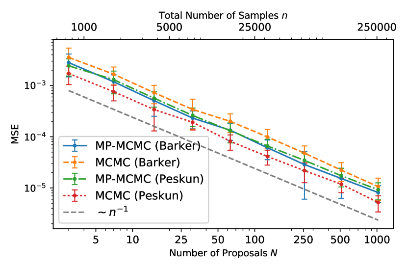
Figure 3: MSE of arithmetic mean for MCMC using Barker’s and Peskun’s acceptance probabilities, and MP-MCMC, resp., sampling from a one-dimensional standard Normal posterior for increasing proposal numbers and sample sizes. The results are based on $25$ MCMC runs, and the error bars correspond to twice a standard deviation, respectively. The difference between all convergence rates is only a constant

3.5 Extensions of standard MP-MCMC

We now consider the following extensions to the MP-MCMC, which can be made to improve sampling performance and which we investigate empirically.

3.5.1 Introducing an auxiliary proposal state

When sampling from $A$ as in (15), the probability of transitioning from $I=i$ to $I=j$ may become small when the number of proposals is large. This is since the acceptance ratio $R(i,j)$ depends not only on the states $\bm{y}_{i}$ and $\bm{y}_{j}$, but all proposed states. One may therefore introduce an auxiliary variable $\bm{z}$ as proposed in [Cal14, Tje04] in order to make proposals of the form $\tilde{\kappa}(\bm{y}_{i},\bm{y}_{\setminus i})=\kappa(\bm{y}_{i},\bm{z})\kappa(\bm{z},\bm{y}_{\setminus i})$. Throughout this work, we make use of this extension for numerical simulations. Assuming that $\kappa$ samples the proposals $\bm{y}_{\setminus i}$ independently from each other, then the acceptance ratio simplifies to

$$R(i,j)=\frac{\pi(\bm{y}_{j})\tilde{\kappa}(\bm{y}_{j},\bm{y}_{\setminus j})}{\pi(\bm{y}_{i})\tilde{\kappa}(\bm{y}_{i},\bm{y}_{\setminus i})}=\frac{\pi(\bm{y}_{j})\kappa(\bm{y}_{j},\bm{z})\kappa(\bm{z},\bm{y}_{i})}{\pi(\bm{y}_{i})\kappa(\bm{y}_{i},\bm{z})\kappa(\bm{z},\bm{y}_{j})}.$$

For a symmetric sample distribution $\kappa$, the acceptance ratio further simplifies to $R(i,j)={\pi(\bm{y}_{j})}/\pi(\bm{y}_{i})$.

3.5.2 Non-reversible transition kernels

In the context of a finite state Markov chain, [ST10] and [TS13] introduce an MCMC method that redefines the transition matrix, allocating the probability of an individual state to the transition probabilities to other states, with the aim of minimising the average rejection rate. In application, the resulting acceptance rate is close to $1$, or even equal to $1$ in many iterations. The resulting transition matrix is no longer reversible; thus, it does not fulfill the detailed balance condition, however it still satisfies the balance condition such that transitioning from one state to another preserves the underlying stationary distribution. The proposed algorithm is immediately applicable for the finite state sampling step in MP-MCMC. The resulting algorithm is a non-reversible MP-MCMC, which preserves the stationary distribution $\pi$ of individual samples. Numerical experiments of this method can be found in Section 3.5.4.

3.5.3 Optimised transition kernels

Given a Markov chain over finitely many proposed states, [Tje04][Section 4] proposes an algorithm that iteratively updates the transition matrix of an MCMC algorithm, starting from Barker’s acceptance probabilities defined on finitely many states. The matrix is updated until only at most one diagonal element is non-zero. Since every update leaves the detailed balance condition valid, the resulting MCMC algorithm is reversible. Again, this method is straightforward to apply in the finite state sampling step of MP-MCMC, resulting in a reversible MP-MCMC, which clearly leaves the stationary distribution $\pi$ of individual samples unaltered. For a single proposal, this algorithm reduces to the usual Metropolis-Hastings. We now consider the performance in numerical experiments, comparing this method to the MP-MCMC with non-reversible transition kernels from 3.5.2 and the standard MP-MCMC.

3.5.4 Empirical results of MP-MCMC extensions

In what follows, we compare the performance of standard MP-MCMC to the MP-MCMC algorithms with improved transition kernels introduced in Section 3.5.2 and Section 3.5.3. As posterior distribution we consider a one-dimensional Gaussian, and for the underlying proposal kernel we use the SmMALA formalism from (16). As measures of performance we consider MSE convergence, acceptance rate and mean squared jumping distance (MSJD) for increasing numbers of proposals. Here, the acceptance rate is defined by the probability of transitioning from one state to any of the $N$ different ones. Further, MSJD $=1/n\sum_{\ell=1}^{n}\|\bm{x}_{n+1}-\bm{x}_{n}\|^{2}$, which is related to measuring the lag $1$ autocorrelation, and can be applied to find the optimal choice of parameters determining the proposal kernel ([PG10]).

Referring to Figure 4, switching from MP-MCMC to any of the MP-MCMC algorithms introduced in the previous two sections increases the average acceptance rate and the MSJD for small proposal numbers significantly, and to a similar extend. While the number of proposals increases, the difference to standard MP-MCMC disappears, as they tend to the same maximal value; for the acceptance rate, this is $1$. At the same time, a performance gain in terms of MSE, referring to Figure 5, is only achieved by switching from the standard MP-MCMC transition kernel to the non-reversible kernel (3.5.2), resulting in an average MSE reduction of ca. $20\%$ overall. Applying the optimised transition algorithm (3.5.3) does not significantly reduce the MSE, i.e. on average less than $5\%$ overall, compared to standard MP-MCMC. This is interesting since it makes the point that, although the choice of proposals is exactly the same, an increased acceptance rate does not imply that the resulting samples are significantly more informative about the posterior. In contrast to this observation we will see in Section 4 that actually, more informative estimates, i.e. exhibiting lower variance, can indeed be achieved by accepting all proposed samples (i.e. acceptance rate $=1$) by suitably weighting them. The number of iterations in the optimisation procedure used to generate the transition kernel from Section 3.5.3 increases significantly with the number of proposals, and therefore the computation cost. To sample a constant number of $250$ iterations in our toy example, we found the cost of performing the optimisation for more than $\approx 125$ proposals prohibitive. For reference and comparison reasons, we displayed the results for proposal numbers only up to this number for standard MP-MCMC and non-reversible MP-MCMC, too. Summarising, we were able to improve the constant in front of the convergence rate by using non-reversible and optimised transition kernels, however not the rate itself.

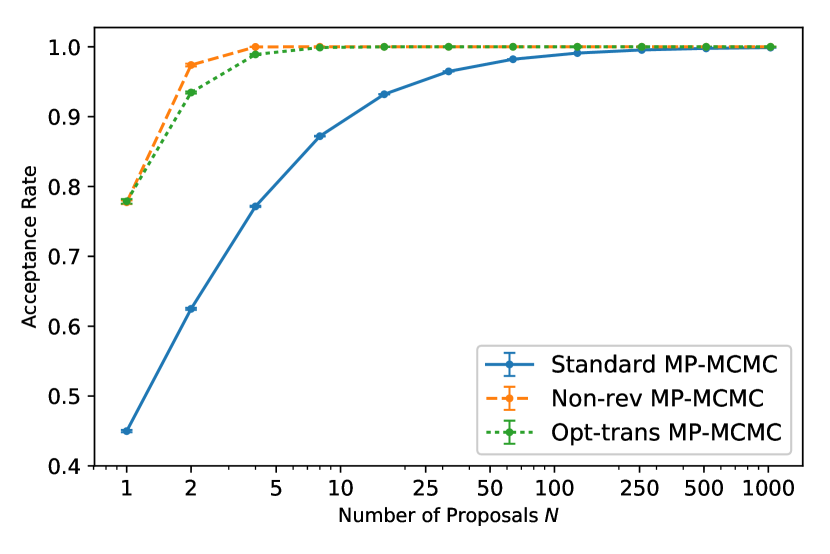
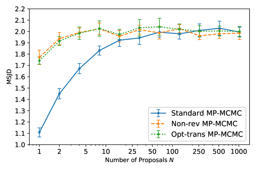
Figure 4: Acceptance rates and MSJD for standard MP-MCMC, MP-MCMC with non-reversible (Non-rev) and optimised transitions (Opt-trans), sampling from a one-dimensional standard Normal posterior for increasing proposal numbers and sample sizes. The results are based on $10$ MCMC runs, and the error bars correspond to twice a standard deviation

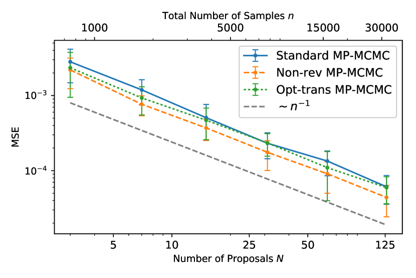
Figure 5: MSE of arithmetic mean for MP-MCMC, MP-MCMC with reversible transitions (Non-rev) and MP-MCMC with optimised transitions (Opt-trans), resp., sampling from a one-dimensional standard Normal posterior for increasing proposal numbers and sample sizes. The results are based on $25$ MCMC runs, and the error bars correspond to twice a standard deviation, resp.

3.6 Limit theorems

In this section, the law of large numbers (LLN), a central limit theorem (CLT), and an expression for the asymptotic variance is derived. Essential for the derivation is the observation that MP-MCMC can be considered as a single Markov chain on the product space of variables $(\bm{y}_{1:N+1},I_{1:M})$, i.e. of proposals and auxiliary variables, when $N$ proposals are generated and $M$ samples are accepted in every iteration, respectively. Here, $\bm{y}_{i}\in\Omega$ and $I_{m}\in\{1,...,N+1\}$ for $i=1,...,N+1$ and $m=1,...,M$. The joint probability on the associated space is given by

$$p(\bm{y}_{1:N+1},I_{1:M}) =p(\bm{y}_{i})\kappa(\bm{y}_{i},\bm{y}_{\setminus{i}})p(I_{1:M}|\bm{y}_{1:N+1})$$

for any $i=1,...,N+1$, where $\kappa(\bm{y}_{i},\bm{y}_{\setminus{i}})$ denotes the proposal distribution. If ergodicity holds, then $p(\bm{y}_{i})=\pi(\bm{y}_{i})$ asymptotically, i.e. the samples collected at each iteration will be distributed according to the target. In that case, updating $(\bm{y}_{1:N+1},I_{1:M})$ leaves the joint distribution invariant. Throughout this section, we will state the main results and definitions while referring to the appendix for the full proof of results to aid readability.

3.6.1 Law of large numbers

Given a scalar-valued function $f$ on $\Omega$, and samples $\bm{x}_{1},\bm{x}_{2},...$ of an MP-MCMC simulation according to Algorithm 1, we wish to prove that $\hat{\mu}_{n}\rightarrow\mu$ a.s., where $\hat{\mu}_{n}=(1/n)\sum_{i}f(\bm{x}_{i})$ and $\mu=\int f(\bm{x})\pi(\bm{x})\mathrm{d}\bm{x}$, which is equivalent to $\hat{\mu}_{n,M,N}\rightarrow\mu$ a.s. for $n\rightarrow\infty$, where

$$\hat{\mu}_{n,M,N}=\frac{1}{nM}\sum_{i=1}^{n}\sum_{m=1}^{M}f(\bm{x}_{m}^{(i)}),$$ (17)

where $\bm{x}_{m}^{(i)}$ denotes the $m$th sample in the $i$th MCMC iteration.

Lemma 3.1 (Law of Large Numbers).

Assuming that the single Markov chain on the product space of accepted samples per iteration, as defined by MP-MCMC, is positive Harris [MT12, 10.1], then the law of large numbers holds true.

Proof.

A proof is given in Appendix B.1. ∎

3.6.2 Central limit theorem

The result we would like to have is the following: given a scalar-valued function $f$ on $\Omega$, and samples $\bm{x}_{1},\bm{x}_{2},...$ of an MP-MCMC simulation, then

$$\sqrt{n}\left(\hat{\mu}_{n}-\mu\right)\xrightarrow{\mathcal{D}}\mathcal{N}(0,\sigma^{2}),$$

for some $\sigma^{2}>0$, which is equivalent to

$$\sqrt{nM}\left(\hat{\mu}_{n,M,N}-\mu\right)\xrightarrow{\mathcal{D}}\mathcal{N}(0,\sigma^{2})\quad\text{for}\quad n\rightarrow\infty,$$

where we used the same notation as in section 3.6.1. In order to prove the CLT we assume the chain to be positive Harris, and that the asymptotic variance can be expressed by the limit of the variances at iteration $n$ for $n\rightarrow\infty$, and is well-defined and positive. Since this seems to be natural to assume, we refer to this assumption by saying the MP-MCMC Markov chain is well-behaved. Since this assumption is not easily verifiable in practice, we also give a formal definition of a uniform ergodicity condition on the Markov chain from [MT12] that ensures the above. For the sake of readability, we refer to Appendix B.2 for this formal condition.

Lemma 3.2 (Central Limit Theorem).

Assuming that the single Markov chain on the product space of accepted samples per iteration, as defined by MP-MCMC, is positive Harris and well-behaved, then the central limit theorem holds true, and the asymptotic variance of the sequence $(f(\bm{x}_{i}))_{i\geq 1}$ is given by

$$\sigma^{2}=\zeta^{(0)}+2\sum_{1\leq\ell<m\leq M}\zeta^{(0)}_{\ell,m}+\frac{2}{M}\sum_{k=1}^{\infty}\sum_{\ell,m=1}^{M}\zeta^{(k)}_{\ell,m}$$

where $\zeta^{(0)}=\operatorname{Var}_{\pi}(f(\bm{x}))$, $\zeta_{m,n}^{(0)}=\operatorname{Cov}(f(\bm{x}_{m}),f(\bm{x}_{n}))$, and $\zeta^{(k)}_{\ell,m}=\operatorname{Cov}(f(\bm{x}_{\ell}^{(i)},f(\bm{x}_{m}^{(i+k)}))$ for any $i,k\in\mathbb{N}$ and $\ell,m=1,...,M\in\mathbb{N}$.

Proof.

For a proof, we refer to Appendix B.2. ∎

3.7 Adaptive MP-MCMC

We now introduce adaptive versions of MP-MCMC within a general framework of adaptivity for Markov chains, and present theory based on [RR07] that allows us to prove ergodicity in adaptive MP-MCMC. Further, an explicit adaptive MP-MCMC method is introduced as Algorithm 2 in Section 3.7.3, for which we prove ergodicity based on the results mentioned above. The performance of IS-MP-MCMC compared to MP-MCMC is then investigated in a simulation study.

3.7.1 Adaptive transition kernels in MP-MCMC

In the following we consider MP-MCMC as a single Markov chain over the accepted samples in one iteration. For any $n\in\mathbb{N}$, let $\bm{Z}_{n}=\bm{x}_{1:M}^{(n)}\in\mathbb{R}^{Md}$ denote the state of the MP-MCMC algorithm at time $n$, i.e. the vector of accepted samples in iteration $n$. Further let $\Gamma_{n}$ denote a $\mathcal{Y}$-valued random variable which determines the kernel choice for updating $\bm{Z}_{n}$ to $\bm{Z}_{n+1}$. We have

$$p(\bm{Z}_{n+1}=\bm{z}_{n+1}|\bm{Z}_{i}=\bm{z}_{i},\Gamma_{i}=\gamma_{i},i=1,...,n) =p(\bm{Z}_{n+1}=\bm{z}_{n+1}|\bm{Z}_{n}=\bm{z}_{n},\Gamma_{n}=\gamma_{n})$$

$$=P_{\gamma_{n}}(\bm{z}_{n},\bm{z}_{n+1}).$$

The dependency of $\Gamma_{n}$ on previous samples and kernel choices, i.e. $\Gamma_{n}|\bm{Z}_{i},\Gamma_{i},i=1,...,n$, will be determined by the corresponding adaptive algorithm. For given starting values $\bm{Z}_{0}=\bm{z},\Gamma_{0}=\gamma$, let

$$P^{(n)}_{\gamma}(\bm{z},\bm{z}_{n})=p(\bm{Z}_{n}=\bm{z}_{n}|\bm{Z}_{0}=\bm{z},\Gamma_{0}=\gamma)$$

denote the corresponding $n$-step conditional probability density of the associated adaptive algorithm. Finally, let us define the total variation between the joint distribution $p$ of variables $\bm{z}=\bm{x}_{1:M}$ and $P^{(n)}_{\gamma}$ by

$$T(\bm{z},\gamma,n)=\left\|P^{(n)}_{\gamma}(\bm{z},\cdot)-p(\cdot)\right\|=\sup_{B}\left|\int_{B}P^{(n)}_{\gamma}(\bm{z},\bm{\tilde{z}})-p(\bm{\tilde{z}})\mathrm{d}\bm{\tilde{z}}\right|.$$

Note that under the joint distribution $p$, all individual samples from every iteration are distributed according to the target $\pi$.

3.7.2 Ergodicity for adaptive chains

Following [RR07], we call the underlying adaptive algorithm ergodic if $T(\bm{z},\gamma,n)\rightarrow 0$ for $n\rightarrow\infty$. Referring to their Theorem 1 and Theorem 2, the following results give sufficient conditions, under which ergodicity holds true. An integral requirement in both theorems is that the changes of the transition kernel due to adaptation tend to zero. To that end, we define the random variable

$$D_{n}=D_{n}(\Gamma_{n+1},\Gamma_{n})=\sup_{\bm{z}}\|P_{\Gamma_{n+1}}(\bm{z},\cdot)-P_{\Gamma_{n}}(\bm{z},\cdot)\|.$$

Note that $D_{n}\rightarrow 0$ for $n\rightarrow\infty$ does not mean that $\Gamma_{n}$ necessarily converges. Also, the amount of adaptation to be infinite, i.e. $\sum_{n}D_{n}=\infty$, is allowed. We note that there exist more general adaptive schemes in the literature ([AFMP11]) which allow that different transition kernels $P_{\gamma}$ have different stationary distributions, however we do not consider these here.

Theorem 3.3 (Theorem 1, [RR07]).

Given an adaptive MP-MCMC algorithm with adaptation space $\mathcal{Y}$ and such that $p$ is the stationary distribution for any transition kernel $P_{\gamma}$, $\gamma\in\mathcal{Y}$. If,

• (Simultaneous Uniform Ergodicity) For any $\varepsilon>0$ there is $N=N(\epsilon)\in\mathbb{N}$ such that $\|P^{(N)}_{\gamma}(\bm{z},\cdot)-p(\cdot)\|\leq\varepsilon$ for any $\bm{z}$ and $\gamma\in\mathcal{Y}$; and

• (Diminishing Adaptation) $D_{n}\rightarrow 0$ for $n\rightarrow\infty$ in probability,

then the adaptive algorithm is ergodic.

The first condition in the previous result is relatively strong, and might not always be verifiable in practice. However, ergodicity still holds if the uniform convergence of $P_{\gamma}$ is relaxed to the following containment condition: roughly speaking, for given starting values for $\bm{Z}_{0}$ and $\Gamma_{0}$, and sufficiently large $n$, $P^{n}_{\gamma}$ is close to $p$ with high probability. To formalise the containment condition, let us define for any $\varepsilon>0$, $\bm{z}\in\mathbb{R}^{Md}$ and $\gamma\in\mathcal{Y}$,

$$M_{\epsilon}(\bm{z},\gamma)=\inf\{n\geq 1:\|P_{\gamma}^{n}(\bm{z},\cdot)-p(\cdot)\|\leq\epsilon\},$$

and state the following ergodicity result.

Theorem 3.4 (Theorem 2, [RR07]).

Consider an adaptive MP-MCMC algorithm that has diminishing adaptation, and let $\bm{z}^{*}\in\Omega^{M},\gamma^{*}\in\mathcal{Y}$. If

• (Containment) For any $\delta>0$ there exists a $N\in\mathbb{N}$ such that $P(M_{\epsilon}(\bm{Z}_{n},\Gamma_{n})\leq N|\bm{Z}_{0}=\bm{z}^{*},\Gamma_{0}=\gamma^{*})\geq 1-\delta$ for any $n\in\mathbb{N}$,

then the adaptive algorithm is ergodic.

The proofs of both previous theorems are based on coupling the adaptive chain with another chain that is adaptive only up to a certain iteration. Referring to [BRR11] containment can actually be derived via the much easier to verify simultaneous polynomial ergodicity or simultaneous geometrical ergodicity. The latter immediately implies containment.

Lemma 3.5 (Asymptotic distribution of adaptive MP-MCMC).

Suppose that either the conditions of Theorem 3.3 or 3.4 are satisfied, then the accepted samples $\bm{x}^{(n)}_{m}\in\Omega$, i.e. the $m$th sample from the $n$th iteration for $n\in\mathbb{N}$ and $m=1,...,M\in\mathbb{N}$, given by $\bm{y}^{(n)}_{I_{m}^{(n)}}=\bm{x}^{(n)}_{m}$, are asymptotically distributed according to the target $\pi$.

Proof.

As the asymptotic behaviour of the Markov chain, defined on states $\bm{x}_{1:M}$, is not influenced by the initial distribution, we may assume the joint target $p$ as initial distribution. The statement then follows immediately. ∎

3.7.3 An adaptive MP-MCMC algorithm

In this section, we consider an adaptive version of the MP-MCMC algorithm, which allows for iterative updates of the proposal covariance. The underlying proposal distribution is formulated in a general fashion, however ergodicity will be proven for the special case of a Normal distribution. In that case, the resulting algorithm can be considered as a generalisation of the adaptive MCMC algorithm introduced by Haario et al. [HST⁺01] allowing for multiple proposals. However, a different covariance estimator than the standard empirical covariance used in [HST⁺01] is applied here: the estimate for the proposal covariance in iteration $n+1$ incorporates information from all previous proposals of iterations $1,2,...,n\in\mathbb{N}$. The proposals are thereby weighted according to the stationary distribution of the auxiliary variable. Note that weighting proposed states does not necessarily decrease the asymptotic variance of the resulting mean estimates ([DJ09]), although in many cases it does ([Fre06, CCK77]). This holds in particular when the number of proposed states is large, which is why we find the weighting estimator preferable over the standard empirical covariance estimate. The resulting method is displayed as Algorithm 2, where we have highlighted the differences compared to Algorithm 1.

Input: Initialise starting point $\bm{x}_{0}=\bm{y}_{1}\in\Omega$, number of proposals $N$, number of accepted samples per iteration $M$, auxiliary variable $I=1$, counter $n=1$, initial mean estimate $\bm{\mu}_{1}$ and covariance estimate $\Sigma_{1}$;

1 for each MCMC iteration $\ell=1,2,...$ do

2       Sample $\bm{y}_{\setminus I}$ conditioned on $I$ and $\Sigma_{\ell}$, i.e., draw $N$ new points from the proposal kernel $\kappa_{\text{\lx@texthl@color{$\Sigma_{\ell}$}}}(\bm{y}_{I},\cdot)=p(\bm{y}_{\setminus I}|\bm{y}_{I},$$\Sigma_{\ell}$$)$ ;

3       Calculate the stationary distribution of $I$ conditioned on $\bm{y}_{1:N+1}$ and $\Sigma_{\ell}$, i.e. $\forall$ $i=1,...,N+1$, $p(I=i|\bm{y}_{1:N+1},$$\Sigma_{\ell}$$)=\pi(\bm{y}_{i})\kappa_{\text{\lx@texthl@color{$\Sigma_{\ell}$}}}(\bm{y}_{{i}},\bm{y}_{\setminus{i}})/\sum_{j}\pi(\bm{y}_{j})\kappa_{\text{\lx@texthl@color{$\Sigma_{\ell}$}}}(\bm{y}_{{j}},\bm{y}_{\setminus{j}})$, which can be done in parallel;

4       for $m=1,...,M$ do

5             Sample new $I$ via the stationary distribution $p(\cdot|\bm{y}_{1:N+1},$$\Sigma_{\ell}$$)$;

6             Set new sample $\bm{x}_{n+m}=\bm{y}_{I}$;

7            

8       end for

9      Update counter $n=n+M$ ;

10       Compute $\tilde{\bm{\mu}}_{\ell+1}=\sum_{i}p(I=i|{{\bm{y}}}_{1:N+1},\Sigma_{\ell})\bm{y}_{i}$;

11       Set $\bm{\mu}_{\ell+1}=\bm{\mu}_{\ell}+\frac{1}{\ell+1}\left(\tilde{\bm{\mu}}_{\ell+1}-\bm{\mu}_{\ell}\right)$;

12       Compute $\tilde{{\Sigma}}_{\ell+1}=\sum_{i}p(I=i|{\bm{y}}_{1:N+1},{{\Sigma}}_{\ell})[{\bm{y}}_{i}-\bm{\mu}_{\ell+1}][{\bm{y}}_{i}-\bm{\mu}_{\ell+1}]^{T}$;

13       Set $\Sigma_{\ell+1}=\Sigma_{\ell}+\frac{1}{\ell+1}(\tilde{\Sigma}_{\ell+1}-\Sigma_{\ell})$;

14      

15 end for

Algorithm 2 Adaptive MP-MCMC
All code altered compared to original MP-MCMC, Algorithm 1, is highlighted

Ergodicity

In what follows we prove ergodicity of the underlying adaptive MP-MCMC method with $\kappa_{\gamma}=N_{\gamma}$, i.e. the proposal distribution being normally distributed, based on the sufficient conditions provided by Theorem 3.4. We prove three different ergodicity results, each based on slightly different requirements. We begin with the case of when proposals are sampled independently of previous samples. In all cases we assume the target $\pi$ to be absolutely continuous with respect to the Lebesgue measure. Further, we say that $\mathcal{Y}$ is bounded if there are $0<c_{1}<c_{2}<\infty$ such that $c_{1}I\leq\gamma\leq c_{2}I$ for any $\gamma\in\mathcal{Y}$, where the “$\leq$” is understood in the usual way considering matrices: For two matrices $A,B\in\mathbb{R}^{n\times n}$, $A\leq B$ means that $B-A$ is positive semi-definite.

Theorem 3.6.

Let us assume that the proposal distribution $\kappa_{\gamma}=N_{\gamma},\gamma\in\mathcal{Y}$, depends on previous samples only through the parameter $\gamma$ but is otherwise independent. If $\mathcal{Y}$ is bounded, then the adaptive MP-MCMC method described by Algorithm 2 is ergodic.

Proof.

The proof is based on Theorem 3.4, and can be found in Appendix C.1. ∎

The following result allows for adapting the mean value of the Normal distribution in addition to its covariance adaptively. The mean value is estimated via weighted proposals, as defined in equation (26).

Corollary 3.7.

Let us assume that the proposal distribution $\kappa_{\gamma}=N_{\gamma},\gamma=(\bm{\mu},\Sigma)\in\mathcal{Y}$ depends on previous samples only through the parameter $\gamma$ but is otherwise independent. If $\mathcal{Y}$ is bounded, i.e. both mean and covariance estimates are bounded, then the adaptive MP-MCMC method described by Algorithm 2 is ergodic.

Proof.

The containment condition follows analogously to the proof for Theorem 3.6. The proof of diminishing adaptation requires integration of $N_{\gamma_{n}+s(\gamma_{n+1}-\gamma_{n})}$, where $\gamma_{n}=(\bm{\mu}_{n},\Sigma_{n})$, similar to equation (44). An estimate similar to (46) follows, where the bound is given by additional constant terms multiplied by either $\|\bm{\mu}_{n+1}-\bm{\mu}_{n}\|$ or $\|\Sigma_{n+1}-\Sigma_{n}\|$. Both terms can be bounded by a constant multiplied by $1/n\rightarrow 0$ for $n\rightarrow\infty$, which concludes the proof. ∎

Now, we consider the case where we assume that the target $\pi$ has bounded support, i.e. there is $S\subset\mathbb{R}^{d}$ with $\lambda(S)<\infty$ such that $\pi(\bm{z})=0$ for any $\bm{z}\not\in S$. The dependence of the proposal distribution on previous samples is not restricted anymore only to the adaptation parameters.

Theorem 3.8.

If $\kappa_{\gamma}=N_{\gamma},\gamma\in\mathcal{Y}$, and the target distribution $\pi$ has bounded support in $\mathbb{R}^{d}$ and its density is continuous, then the adaptive MP-MCMC method described by Algorithm 2 is ergodic.

Proof.

The proof is again based on Theorem 3.4, and can be found in Appendix C.2. ∎

Corollary 3.9.

Under the same conditions as in Theorem 3.8, except that we do not assume continuity, the statement still holds true if we instead assume that $\pi$ is bounded from above and below on its support, i.e. $\exists\ 0<\eta\leq\rho<\infty$ such that

$$\eta\leq\pi(\bm{x})\leq\rho$$ (18)

for any $\bm{x}$ in the support of $\pi$.

Proof.

The statement follows similarly to the proof of Theorem 3.8, except that the boundedness of the transition probability on the finite state chain in (39) is ensured by (18) instead of by continuity. ∎

In the following case, we waive both the independence as well as the bounded support condition, however we require a few other assumptions to show ergodicity in Theorem 3.10, among which is the positivity of the target distribution. Therefore, Theorem 3.8 and Theorem 3.10 can be considered as complementing each other. The containment condition is generally hard to prove in practise wihtout further assumptions, and for the case of unbounded support of a dependent proposal kernel we have not managed to achieve such a direct proof. Hence, we turned to [CGŁ⁺15] which states sufficient and practically verifiable assumptions under which the rather technical containment condition holds true. More precisely, it is assumed that the underlying Markov chain can only jump within a finite distance of any current sample. Furthermore, the transition kernel is only adapted within a compact region of the state space. Outside of this region, a fixed proposal kernel is used, which defines a chain that converges to the correct stationary distribution. In what follows, $K_{D}$ is the set of all states within an Euclidean distance $D$ from $K$ for any bounded set $K\subset\Omega^{M}$.

Assumption 1 (Bounded jump condition).

Assume that there is a $D<\infty$ such that

$$P_{\gamma}(\tilde{\bm{z}},\{\bm{z}\in\Omega^{M}:\|\bm{z}-\tilde{\bm{z}}\|\leq D\})=1\quad\forall\ \tilde{\bm{z}}\in\Omega^{M},\gamma\in\mathcal{Y}.$$ (19)

Assumption 2 (Non-adaptive kernel condition).

Assume that there is a bounded $K\subset\Omega^{M}$ such that

$$P_{\gamma}(\bm{z},B)=P(\bm{z},B)\quad\forall\ B\in\mathcal{B}(\Omega^{M}),\bm{z}\in\Omega^{M}\setminus{K},$$ (20)

for some fixed transition kernel $P$ defining a chain that converges to the correct stationary distribution $p$ on $\Omega^{M}$ in total variation for any initial point. Further, it is assumed that

$$\exists\ M<\infty\quad\text{such that}\quad P(\tilde{\bm{z}},\mathrm{d}\bm{z})\leq M\lambda(\mathrm{d}\bm{z}),$$ (21)

for any $\tilde{\bm{z}}\in K_{D}\setminus{K}$ and any $\bm{z}\in K_{2D}\setminus{K_{D}}$, where $D$ is as in Assumption 1. Moreover, there are $\varepsilon,\delta>0$ such that

$$P(\tilde{\bm{z}},\mathrm{d}\bm{z})\geq\varepsilon\lambda(\mathrm{d}\bm{z})$$ (22)

for any $\tilde{\bm{z}},\bm{z}$ with $\|\tilde{\bm{z}}-\bm{z}\|<\delta$ in some bounded rectangle contained in $\Omega^{M}$ and that contains $K_{2D}\setminus{K_{D}}$.

We remark that the conditions from equation (19) and (20) are easily enforced upon Algoritm 2 by making the following changes to the algorithm: if a proposal is generated that does not satisfy the first equation simply remove the proposal and sample a new proposal and repeat until it the condition satisfied. In order to ensure the second assumption, set the proposal distribution to a fixed Gaussian distribution outside of the set $K$. One easily verifies that the remaining conditions (21) and (22) are then also satisfied.

Theorem 3.10 (Ergodicity of adaptive MP-MCMC).

Let the conditions from Assumption 1 and Assumption 2 be satisfied. Further, let $\pi$ be continuous and positive, $\Omega\subset\mathbb{R}^{d}$ open, and $\mathcal{Y}$ be bounded. Then, the adaptive MP-MCMC method described by Algorithm 2 is ergodic.

Proof.

For a proof, we refer to Appendix C.3. ∎

3.7.4 Adaptive MP-MCMC with non-Gaussian proposals

The question arises what theoretical guarantees hold if the underlying proposal distribution is not Gaussian, different to the case of Algorithm 2. As before, we may proceed by proving diminishing adaptation and containment. According to [CGŁ⁺15], the first condition, which basically says that the changes in the process become smaller and smaller as time goes by, is typically simple to achieve by carefully choosing the proposal distribution and designing what adaptation is used. As pointed out above, the second condition is hard to prove directly without further assumptions. However, by raising the further two conditions 1 and 2 upon the transition kernel ensures containment. Both conditions are closely related to the choice of the proposal distribution and the design of adaptation, which both are in the hand of the user. This suggests that for algorithms that apply a different adaptation as in Algorithm 2 and have non-Gaussian proposals similar results as in the last section can be achieved.

4 Pseudo-random MP-MCMC with Importance Sampling

In MP-MCMC, samples are drawn from a Markov chain defined on all $N+1$ proposals in each iteration. These samples are in turn typically used to compute some quantity of interest, which can be expressed as an integral with respect to the target. The same can be achieved by weighting all proposed states from each iteration appropriately without any sampling on the finite state chain. Before explaining the details of the resulting method, we state an intuitive motivation for why we should make use of weighting.

4.1 Introduction and motivation

We start by arguing that increasing the number of accepted samples per iteration while keeping the number of proposals and the number of outer iterations constant is typically beneficial in terms of reducing the empirical variance of estimates. In order to see this, note that for the variance $\sigma_{n,M,N}^{2}$ of the mean estimator $\hat{\mu}_{n,M,N}$ for $n,M,N\in\mathbb{N}$ it holds that

$$\sigma_{n,M,N}^{2} =\frac{1}{n}\sum_{i=1}^{n}\operatorname{Var}\left(F\left(\bm{x}_{1:M}^{(i)}\right)\right)$$

$$\quad\quad+\frac{2}{n}\sum_{1\leq i<j\leq n}\operatorname{Cov}\left(F\left(\bm{x}_{1:M}^{(i)}\right),F\left(\bm{x}_{1:M}^{(j)}\right)\right),$$

where $\bm{x}_{1:M}^{(i)}$ states the accepted set of $M$ samples in the $i$th iteration, and $F$ is defined as

$$F(\bm{x}_{1:M})=\frac{1}{M}\sum_{m=1}^{M}f(\bm{x}_{m}).$$ (23)

Further,

$$\operatorname{Var}\left(F\left(\bm{x}_{1:M}^{(i)}\right)\right)=\frac{1}{M}\operatorname{Var}\left(f(\bm{x}^{(i)})\right)+\frac{1}{M^{2}}\sum_{\ell,m=1}^{M}\operatorname{Cov}\left(f(\bm{x}^{(i)}_{\ell}),f(\bm{x}^{(i)}_{m}\right).$$

Clearly, the first term decreases with increasing $M$. For the second term, note that for sufficiently large $M$, the relative frequency of accepting a proposal $\bm{y}_{\ell}^{(i)}$ as a sample among all $N+1$ proposals of the $i$th iteration is approximately equal to the stationary distribution $p(I=\ell|\bm{y}_{1:N+1}^{(i)})$. Therefore,

$$\begin{split}\frac{1}{M^{2}}\sum_{\ell,m=1}^{M}\operatorname{Cov}\left(f(\bm{x}^{(i)}_{\ell}),f(\bm{x}^{(i)}_{m}\right)&\approx\sum_{\ell,m=1}^{N+1}p(I=\ell|\bm{y}^{(i)}_{1:N+1})p(I=m|\bm{y}^{(i)}_{1:N+1})\\ &\quad\quad\cdot\operatorname{Cov}\left(f(\bm{y}_{\ell}^{(i)}),f(\bm{y}_{m}^{(i)})\right),\end{split}$$ (24)

which does not depend on $M$. Similarly,

$$\operatorname{Cov}\left(F\left(\bm{x}_{1:M}^{(i)}\right),F\left(\bm{x}_{1:M}^{(j)}\right)\right) =\frac{1}{M^{2}}\sum_{\ell,m=1}^{M}\operatorname{Cov}\left(f(\bm{x}_{\ell}^{(i)}),f(\bm{x}_{m}^{(j)})\right)$$

$$\begin{split}&\approx\sum_{\ell,m=1}^{N+1}p(I=\ell|\bm{y}^{(i)}_{1:N+1})p(I=m|\bm{y}^{(j)}_{1:N+1})\\ &\quad\quad\cdot\operatorname{Cov}\left(f(\bm{y}_{\ell}^{(i)}),f(\bm{y}_{m}^{(j)})\right),\end{split}$$ (25)

for sufficiently large $M$, which again is independent of $M$. In summary, we have

$$\sigma_{M,N,n}^{2}\gtrsim\sigma_{M^{\prime},N,n}^{2}\quad\quad\text{for}\quad M^{\prime}>M.$$

An increase of $M$ for a given iteration and increasing proposal numbers $N$ has been investigated numerically: for any $N$, we analysed the empirical variance of a mean estimate for $M\in\{2^{\alpha}N:\alpha=0,...,4\}$. The case of $\alpha=\infty$ corresponds to MP-MCMC with importance sampling (IS-MP-MCMC), described by Algorithm 3. The underlying target is a one-dimensional Gaussian distribution, and we set the proposal sampler to the SmMALA kernel defined in (16). The corresponding results are displayed in Figure 6 (left). Indeed, an increase in $M$ yields a decrease in variance as expected. At the same time, the magnitude of the reduction in variance also decreases with increasing $M$. The limiting case, which corresponds to accepting all proposals and then suitably weighting them, exhibits the lowest variance. In some sense this contrast the general observation that an increased acceptance rate in MCMC does not necessarily produce more informative estimates.

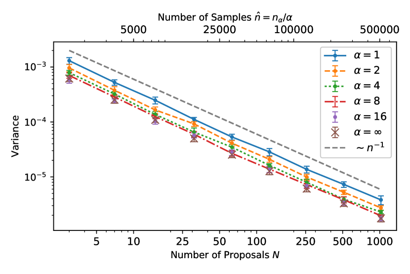
Figure 6: Variance convergence of the arithmetic mean from MP-MCMC with Riemannian SmMALA proposals on a one-dimensional standard Normal posterior for increasing proposal numbers $N$ and for changing number of accepted proposals per iteration $M=\operatorname{const}$ (right). Results based on $10$ MCMC simulations. The error bars corresponds to three times a standard deviation

In the limiting case, $M\rightarrow\infty$, the two approximations in (24)-(25) become equalities, and sampling from the finite state chain in one iteration corresponds in principle to accepting all proposals $\bm{y}_{1:N+1}$ but weighting each $\bm{y}_{i}$ according to $p(I=i|\bm{y}_{1:N+1})$. This can be formalised as an importance sampling approach for MCMC with multiple proposals. A visualisation of this method is given in Figure 7. Due to the considerations above, this approach typically produces a smaller variance than the standard MP-MCMC, where $p(I|\bm{y}_{1:N+1})$ is used to sample from the finite state chain in every iteration.

Figure 7: In IS-MP-MCMC, we associate to every proposal ${\bm{y}}^{(\ell)}_{i}$ its weight $w^{(\ell)}_{i}=p(I^{(\ell)}=i|\bm{y}_{1:N+1}^{(\ell)})$, thereby prioritising proposals that are most informative about the posterior

4.1.1 Waste-Recyling

Using a different heuristic, [Tje04] introduced the importance sampling technique from above, as well as [CCK77, Fre04, Fre06, DJ09]. In some of the literature, e.g. [Fre06], this technique is referred to as Waste-Recycling due to the fact that every proposal is used, including the ones rejected by MCMC. Compared to standard MP-MCMC, i.e. using Barker’s acceptance probabilities, and when $M=1$, IS-MP-MCMC has been shown to be superior in terms of asymptotic variance [DJ09]. However, [DJ09] construct an example for the single proposal case where importance sampling (Waste-recycling) can perform worse than the Metropolis-Hastings algorithm if Peskun’s acceptance probability is employed.

4.2 Importance sampling MP-MCMC Algorithms

We now present the importance sampling version of MP-MCMC to estimate the integral $\bm{\mu}=\bm{\mu}(f)=\int f(\bm{x})\pi(\bm{x})\mathrm{d}\bm{x}$ for a given function $f:\Omega\rightarrow\mathbb{R}^{d^{\prime}}$ for $d^{\prime}\in\mathbb{N}$. In every iteration, each proposal $f(\bm{y}_{i})$ is weighted according to the stationary distribution $p(I=i|\bm{y}_{1:N+1})$. The sum of weighted proposals yields an estimate for the mean $\bm{\mu}$. The resulting method is described by Algorithm 3.

Note that this defines a Markov chain driven algorithm: in every iteration, according to $p(\cdot|{{\bm{y}}}_{1:N+1})$ one sample from the $N+1$ proposals is drawn (line $6$), conditioned on which then $N$ new proposals are drawn in the subsequence iteration. This chain corresponds to the standard MP-MCMC with $M=1$. When we mention the underlying Markov chain corresponding to importance sampling MP-MCMC, we refer to this chain.

The importance sampling estimator $\bm{\mu}_{L}=\bm{\mu}_{L}(f)$ for $L\in\mathbb{N}$ can also be written as

$$\bm{\mu}_{L}=\frac{1}{L}\sum_{\ell=1}^{L}\sum_{i=1}^{N+1}w^{(\ell)}_{i}f({\bm{y}}_{i}^{(\ell)}),$$ (26)

where $w^{(\ell)}_{i}=p(I=i|{{\bm{y}}}_{1:N+1}^{(\ell)})$ for $i=1,...,N+1$ and $\ell=1,...,L$.

Input: Initialise starting point (proposal) $\bm{y}_{1}\in\Omega$, number of proposals $N$, auxiliary variable $I=1$, integrand $f$ and initial mean estimate $\bm{\mu}_{1}=\bm{\mu}_{1}(f)$;

1 for each MCMC iteration $\ell=1,2,...$ do

2       Sample ${\bm{y}}_{\setminus I}$ conditioned on $I$, i.e., draw $N$ new points from the proposal kernel $\kappa({\bm{y}}_{I},\cdot)=p({\bm{y}}_{\setminus I}|{\bm{y}}_{I})$ ;

3       Calculate the stationary distribution of $I$ conditioned on ${\bm{y}}_{1:N+1}$, i.e. $\forall$ $i=1,...,N+1$, $p(I=i|{{\bm{y}}}_{1:N+1})=$ $\pi({{\bm{y}}}_{i})\kappa({{\bm{y}}}_{{i}},{{\bm{y}}}_{\setminus{i}})/\sum_{j}\pi({{\bm{y}}}_{j})\kappa({{\bm{y}}}_{{j}},{{\bm{y}}}_{\setminus{j}})$, which can be done in parallel;

4       Compute $\tilde{\bm{\mu}}_{\ell+1}=\sum_{i}p(I=i|{{\bm{y}}}_{1:N+1})f({{\bm{y}}}_{i})$;

5       Set $\bm{\mu}_{\ell+1}=\bm{\mu}_{\ell}+\frac{1}{\ell+1}\left(\tilde{\bm{\mu}}_{\ell+1}-\bm{\mu}_{\ell}\right)$;

6       Sample new $I$ via the stationary distribution $p(\cdot|{{\bm{y}}}_{1:N+1})$;

7      

8 end for

Algorithm 3 Importance sampling MP-MCMC
All code altered compared to original MP-MCMC, Algorithm 1, is highlighted

4.2.1 Lack of samples representing $\pi$

Despite the amenable properties of the importance sampling approach for MP-MCMC, compared to the standard MP-MCMC, Algorithm 3 has the disadvantage that it does not produce samples that are directly informative and approximately distributed according to a target, but rather an approximation of an integral with respect to the target instead.

4.2.2 Adaptive importance sampling

In many situations, it may make sense to adaptively learn the proposal kernel about the target, based on the past history of the algorithm. We therefore extend Algorithm 3 to make use of importance sampling, which is described in Algorithm 4. This can be achieved by making use of estimates for global parameters which are informative about the target, e.g. mean and covariance. Clearly, the Markov property of the stochastic process resulting from this approach will not hold. This is generally problematic for convergence, and thus for the consistency of the importance sampling estimate. However, given the usual diminishing adaptation condition, i.e. when the difference in subsequent updates converges to zero, and some further assumptions on the transition kernel, referring to Section 3.7, consistency can be shown. Since in the importance sampling method there are no actual samples generated following the target distribution asymptotically, but an estimate for an integral over the target, we understand asymptotic unbiasedness of the resulting estimate when we talk about consistency ([DJ09]).

With the same notation as in Section 4.3, we assume that the proposal kernel $\kappa=\kappa_{\gamma}$ depends on a parameter $\gamma$ belonging to some space $\mathcal{Y}$. Examples of $\gamma$ are mean and covariance estimates of the posterior distribution. A proof for asymptotic unbiasedness in the case where $\kappa$ is the Normal distribution is given in Corollary 4.2. In the particular case where sampling proposals depends on previous samples only though the adaptation parameters but is otherwise independent, i.e. $\kappa_{\gamma}(\bm{x},\cdot)=\kappa_{\gamma}(\cdot)$ $\forall\bm{x}\in\Omega$, we found the use of adaptivity most beneficial in applications for the Bayesian logistic regression from 5.5 and Bayesian linear regression from 5.5, compared to dependent proposals.

Input: Initialise starting point (proposal) $\bm{y}_{1}$, number of proposals $N$, auxiliary variable $I=1$, integrand $f$, initial mean estimate $\bm{\mu}_{1}=\bm{\mu}_{1}(f)$ and covariance estimate $\Sigma_{1}$;

1 for each MCMC iteration $\ell=1,2,...$ do

2       Sample ${\bm{y}}_{\setminus I}$ conditioned on $I$ and $\Sigma_{\ell}$, i.e., draw $N$ new points from the proposal kernel $\kappa_{\text{\lx@texthl@color{$\Sigma_{\ell}$}}}({\bm{y}}_{I},\cdot)=p({\bm{y}}_{\setminus I}|{\bm{y}}_{I},$$\Sigma_{\ell})$ ;

3       Calculate the stationary distribution of $I$ conditioned on ${\bm{y}}_{1:N+1}$ and $\Sigma_{\ell}$, i.e. $\forall$ $i=1,...,N+1$, $p(I=i|{{\bm{y}}}_{1:N+1},$$\Sigma_{\ell}$)$=$ $\pi({{\bm{y}}}_{i})\kappa_{\text{\lx@texthl@color{$\Sigma_{\ell}$}}}({\bm{y}}_{i},{{\bm{y}}}_{\setminus{i}})/\sum_{j}\pi({{\bm{y}}}_{j})\kappa_{\text{\lx@texthl@color{$\Sigma_{\ell}$}}}({\bm{y}}_{j},{{\bm{y}}}_{\setminus{j}})$, which can be done in parallel;

4       Compute $\tilde{\bm{\mu}}_{\ell+1}=\sum_{i}p(I=i|{{\bm{y}}}_{1:N+1}$, $\Sigma_{\ell}$$)f({{\bm{y}}}_{i})$;

5       Set $\bm{\mu}_{\ell+1}=\bm{\mu}_{\ell}+\frac{1}{\ell+1}\left(\tilde{\bm{\mu}}_{\ell+1}-\bm{\mu}_{\ell}\right)$;

6       Sample new $I$ via the stationary distribution $p(\cdot|{{\bm{y}}}_{1:N+1},$ $\Sigma_{\ell})$;

7       Compute $\tilde{{\Sigma}}_{\ell+1}=\sum_{i}p(I=i|{\bm{y}}_{1:N+1},{{\Sigma}}_{\ell})[{\bm{y}}_{i}-\bm{\mu}_{\ell+1}][{\bm{y}}_{i}-\bm{\mu}_{\ell+1}]^{T}$;

8       Set ${\Sigma}_{\ell+1}={\Sigma_{\ell}}+\frac{1}{\ell+1}(\tilde{{\Sigma}}_{\ell+1}-{\Sigma}_{\ell})$;

9      

10 end for

Algorithm 4 Adaptive importance sampling MP-MCMC
All code altered compared to IS-MP-MCMC, Algorithm 3, is highlighted

4.3 Asymptotic unbiasedness of IS-MP-MCMC

In this section, we prove the asymptotic unbiasedness of mean and covariance estimates from Algorithm 3 and Algorithm 4, respectively. We further refer to an existing result in the literature which states the asymptotic normality of the IS-MP-MCMC mean estimator.

Lemma 4.1 (Asymptotic unbiasedness of IS-MP-MCMC).

Given that the underlying Markov chain is positive Harris,, the IS-MP-MCMC sequence of estimators $(\bm{\mu}_{L})_{L\geq 1}$ from Algorithm 3 is asymptotically unbiased.

Proof.

The statement is proven in Appendix C.4. ∎

Lemma 4.1 states that after having discarded a sufficiently large burn-in period of (weighted) samples, the importance sampling estimator defined by the remaining samples is unbiased.

Corollary 4.2 (Asymptotic unbiasedness of adaptive IS-MP-MCMC).

Under any of the conditions stated in Theorem 3.6, Theorem 3.8 or Theorem 3.10, the sequence of estimators $(\bm{\mu}_{L})_{L\geq 1}$ from Algorithm 4 is asymptotically unbiased.

Proof.

Ergodicity of the adaptive MP-MCMC follows by the respective theorem used. Thus, we may argue analogously to the proof of Lemma 4.1. ∎

Corollary 4.3.

Under the same conditions as in Lemma 4.1, the sequence of covariance estimates $({\Sigma}_{L})_{L\geq 1}$ from Algorithm 2 and Algorithm 4 is asymptotically unbiased.

Proof.

For a proof, we refer to Appendix C.5. ∎

The following result states that IS-MP-MCMC produces asymptotically normal estimates, that outperform standard MP-MCMC (using Barker’s acceptance probabilities (14)) for $M=1$ in terms of their asymptotic variance. Thus, making use of all proposals in every iteration is better than accepting only a single one per iteration.

Lemma 4.4 (Proposition 4.1, [DJ09]).

The IS-MP-MCMC sequence of estimators $(\bm{\mu}_{L})_{L\geq 1}$ from Algorithm 3 is asymptotically normal. Its asymptotic variance is smaller or equal to the asymptotic variance of MP-MCMC with $M=1$.

4.4 Bayesian logistic regression

In what follows we consider the Bayesian logistic regression model as formulated in [GC11]. The dependent variable $y$ is categorical with binary outcome. The probability of $y$ is based on predictor variables defined by the design matrix $X\in\mathbb{R}^{n\times d}$, and is given by $P(y=1|X,\bm{\theta})=\sigma(X\bm{\theta})$ and $P(y=0|X,\theta)=1-\sigma(X\theta)$, where $\sigma$ denotes the logistic function. Our goal is to perform inference over the regression parameter $\bm{\theta}\in\mathbb{R}^{d}$, which has the Gaussian prior $\pi(\theta)=\mathcal{N}(\bm{0},\alpha\mathbf{I}_{d})$, with $\alpha=100$. For further details, we refer to [GC11]. For the above mentioned logistic regression, there are overall $5$ different underlying data sets of varying dimensionality at our disposal, which we denote by Ripley (d=3), Pima (d=8), Heart (d=14), Australian (d=15) and German (d=25). For brevity, we consider only the lowest-dimensional model data in the following experiments. In later experiments where we use a QMC seed to run the above introduced MCMC algorithms, we investigate their performance on all data sets.

4.4.1 Empirical results

We now compare the performance of IS-MP-MCMC and adaptive IS-MP-MCMC in the context of the Bayesian logistic regression model introduced above. As a reference we also consider the standard, i.e. single proposal, random-walk Metropolis-Hastings algorithm. To ensure fairness the total number of samples $n$ produced by the single and multiple proposal algorithms are equal, i.e. $n=LN$ if $L$ denotes the number if iterations and $N$ the number of proposals in the multiple proposal case.

In all algorithms we choose a Gaussian proposal sampler. For the importance sampling methods, proposals are generated independently of previous samples. As an initial proposal mean and covariance a rough estimate of the posterior mean and covariance is employed. The former is used to initialise the Metropolis-Hastings algorithm. In the adaptive algorithm, proposal mean and covariance estimates are iteratively updated after every iteration. The results for the empirical variance associated to the posterior mean estimates in the above mentioned algorithms are displayed in Figure 8. The importance sampling algorithms outperform Metropolis-Hastings by over an order of magnitude. Further, the adaptive algorithm produces slightly better results than the non-adaptive importance sampler, with an average empirical variance reduction of over $20\%$.

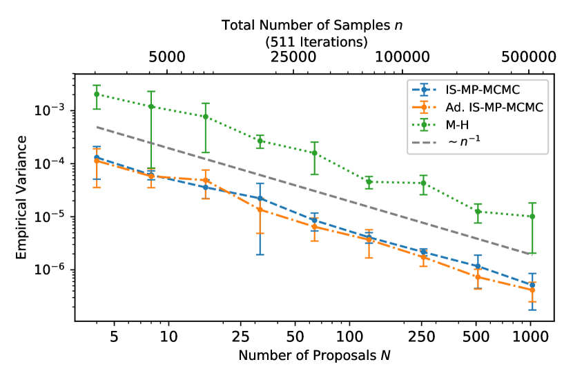
Figure 8: Empirical variance of the arithmetic mean for IS-MP-MCMC and adaptive IS-MP-MCMC in the Bayesian logistic regression model from [GC11] ($d=3$) for increasing proposal numbers $N$ and total number of samples $n$; also displayed is Metropolis-Hastings (M-H) for reference. Here, M-H was tuned to an approximately optimal acceptance rate of $20$-$25\%$. Results are based on $25$ MCMC simulations. The error bars correspond to three times a standard deviation

5 Combining QMC with MP-MCMC

In this section, we introduce a general framework for using CUD numbers in the context of MP-MCMC, leading to a method we shall call MP-QMCMC. The motivation for this is that since in each iteration $N$ proposals are provided as alternatives to any current state, all of which contribute to the exploration of the underlying local region of state space, we might reasonably expect a higher gain using QMC points for these than for the single proposal case, where there is always only one alternative to the current state. We prove the consistency of our proposed method and illustrate in numerical experiments an increased performance. We also extend our methodology to importance sampling, for which we observe an improved rate of convergence of close to $n^{-2}$ in simulations, instead of the standard MCMC rate of $n^{-1}$ in MSE. Summarising, we generalise Algorithms 1, 3 and 4 to using any choice of CUD numbers as the driving sequence.

5.1 MP-QMCMC

We now introduce the above mentioned MP-QMCMC algorithm, and subsequently prove its consistency based on regularity conditions. Moreover, we investigate the algorithm’s performance by simulations based on the Bayesian logistic regression model introduced in Section 4.4 and $5$ different underlying data sets. We conclude the section with some practical advice on effectively harvesting the benefits of QMC based MCMC algorithms.

5.1.1 Algorithm description

We exchange the usual driving sequence of pseudo-random numbers by CUD numbers. In every iteration, this comprises two situations: in the first, proposals are generated, and in the second one, given the transition matrix for the finite state chain on the proposed states, auxiliary variables are generated. In order to create the $N$ new proposals in $\Omega\subset\mathbb{R}^{d}$ we utilise $Nd$ numbers from a CUD sequence in $(0,1)$. Further, to sample from the finite state chain $M$ times we utilise another $M$ numbers from the underlying CUD sequence. Our algorithm is designed such that the entire CUD sequence is used, thereby making full use of the spatial homogeneity. A pseudo-code description of the resulting MP-QMCMC is given in Algorithm 5, which represents an extension of Algorithm 1 to using any choice of CUD numbers as the driving sequence.

The function $\Psi_{\bm{y}_{I}}$ in line three of the algorithm denotes the inverse of the cumulative distribution function (CDF) of the proposal distribution. Thus, given $N$ vectors $\bm{u}_{i}\in(0,1)^{d}$, represented by the joint vector $\bm{u}=(\bm{u}_{1},...,\bm{u}_{N})$, $\Psi_{\bm{y}_{I}}$ assigns $\bm{u}$ to $N$ new proposals $\bm{y}_{\setminus{I}}\in\Omega^{N}$. Practically, each sub-vector $\bm{u}_{i}$ of $\bm{u}$ is assigned to one new proposal. For $d>1$, sampling via inversion can be expressed as iteratively sampling from the one-dimensional conditional proposal distribution, i.e. sampling the first coordinate of the new proposal via inversion of the conditional CDF of the first coordinate, then given that coordinate sampling the second one accordingly and so on.

Input: Initialise starting point ${\bm{x}}_{0}=\bm{y}_{1}\in\Omega$, number of proposals $N$, number of accepted samples per iteration $M$, auxiliary variable $I=1$, counter $n=1$ and number of MCMC iterations $L$;

1 Generate a CUD sequence $u_{1},...,u_{L(Nd+M)}\in(0,1)$;

2 for each MCMC iteration $\ell=1,...,$$L$  do

3       Set $\bm{u}=(u_{(\ell-1)(Nd+M)+1},...,u_{(\ell-1)(Nd+M)+Nd})\in(0,1)^{Nd}$, and sample $\bm{y}_{\setminus I}$ conditioned on $I$, i.e., draw $N$ new points from $\kappa(\bm{y}_{I},\cdot)=p(\bm{y}_{\setminus I}|\bm{y}_{I})$ by the inverse $\Psi_{\bm{y}_{I}}(\bm{u})$ ;

4       Calculate the stationary distribution of $I$ conditioned on $\bm{y}_{1:N+1}$, i.e. $\forall$ $i=1,...,N+1$, $p(I=i|\bm{y}_{1:N+1})=$ $\pi(\bm{y}_{i})\kappa(\bm{y}_{i},\bm{y}_{\setminus{i}})/\sum_{j}\pi(\bm{y}_{j})\kappa(\bm{y}_{j},\bm{y}_{\setminus{j}})$, which can be done in parallel;

5       Set $\bm{v}^{\prime}=(u_{(\ell-1)(Nd+M)+Nd+1},...,u_{\ell(Nd+M)})\in(0,1]^{M}$;

6       for $m=1,...,M$ do

7             If $v^{\prime}_{m}\in(\gamma_{j-1},\gamma_{j}]$, where $\gamma_{j}=\sum_{i=1}^{j}p(I=i|\bm{y}_{1:N+1})$ for $j=1,...,N+1$ and $\gamma_{0}:=0$, set $x_{n+m}=\bm{y}_{j}$;

8            

9       end for

10      Update counter $n=n+M$

11 end for

Algorithm 5 MP-QMCMC
All code altered compared to original (pseudo-random) MP-MCMC, Algorithm 1, is highlighted

5.1.2 Consistency

In the following section we prove that MP-MCMC driven by CUD numbers instead of pseudo-random numbers produces samples according to the correct stationary distribution under regularity conditions. In general, using CUD points is not expected to yield consistency for any MCMC algorithm that is not ergodic when sampling with IID numbers [CDO⁺11]. Similar to Chen et al., our proof is based on the so called Rosenblatt-Chentsov transformation.

Rosenblatt-Chentsov transformation

Let us assume that there is a generator $\psi_{\pi}$ that produces samples according to the target distribution $\pi$, i.e. $\psi_{\pi}(\bm{u})=\bm{x}\sim\pi$ if $\bm{u}\sim\mathcal{U}[0,1]^{d}$. For example, $\psi_{\pi}$ could be based on the inversion method applied to the one-dimensional conditional distributions of the target, assumed that they are available. For $n=LM$ the $N$-proposal Rosenblatt-Chentsov transformation of $\bm{u}_{0}\in(0,1)^{d}$ and a finite sequence of points $u_{1},...,u_{L(Nd+M)}\in(0,1)$ is defined as the finite sequence $\bm{x}_{0},\bm{x}_{1},...\bm{x}_{LM}\in\Omega$, where $\bm{x}_{0}=\psi_{\pi}(\bm{u}_{0})$ and $\bm{x}_{1},...\bm{x}_{LM}$ are generated according to Algorithm 5 using $u_{1},...,u_{L(Nd+M)}\in(0,1)$ as driving sequence and $\bm{x}_{0}$ as initial point.

Since the standard version of MP-MCMC fulfills the detailed balance condition, updating samples preserves the underlying stationary distribution $\pi$. Thus, whenever one sample follows $\pi$, all successive samples follow $\pi$. That means, whenever $\bm{x}_{0}\sim\pi$, all points generated by MP-MCMC follow $\pi$. If the sequence of points $u_{1},...,u_{L(Nd+M)}$ in the $N$-proposal Rosenblatt-Chentsov transformation are uniformly distributed, then this holds for the samples generated by Algorithm 5, too. This observation will be used in the following to show the consistency of MP-QMCMC. Before that, we formulate some regularity condition that will be used in the proof.

Regularity conditions

Similarly to [CDO⁺11], the consistency proof which is given below relies on two regularity conditions. The first one defines coupling properties of the sampling method, and the second one suitable integrability over the sample space.

1) Coupling: Let $\phi(\tilde{\bm{x}}_{M},(u_{1},...,u_{Nd+M}))=(\bm{x}_{1},...,\bm{x}_{M})$ denote the innovation operator of MP-MCMC, which assigns to the last sample $\tilde{\bm{x}}_{M}$ of the current iteration the $M$ new samples from the subsequent iteration. Let $\mathcal{C}\subset(0,1)^{Nd+M}$ have positive Jordan measure. If for any $\bm{u}\in\mathcal{C}$ it holds $\phi(\bm{x},\bm{u})=\phi(\bm{x}^{\prime},\bm{u})$ $\forall$ $\bm{x},\bm{x}^{\prime}\in\Omega$, then $\mathcal{C}$ is called a coupling region.
Let $\bm{z}_{i}=\phi(\bm{x},\bm{u}_{i})$ and $\bm{z}_{i}^{\prime}=\phi(\bm{x}^{\prime},\bm{u}_{i})$ be two iterations from Algorithm 5 based on the same innovations $\bm{u}_{i}\in(0,1)^{Nd+M}$ but possibly different current states $\bm{x}$ and $\bm{x}^{\prime}$, respectively.. If $\bm{u}_{i}\in\mathcal{C}$, then $\bm{z}_{j}=\bm{z}_{j}^{\prime}$ for any $j\geq i$. In other words, if $\bm{u}_{i}\in\mathcal{C}$, two chains with the same innovation operator but potentially different starting points coincide for all $j\geq i$. As a non-trivial example, standard MP-MCMC with independent proposal sampler has a coupling see Lemma 5.2.

2) Integrability: For $k\geq 1$, let $\bm{x}_{k}=\bm{x}^{i}_{j}=\bm{x}^{i}_{j}(\bm{u}^{1},...,\bm{u}^{i})$ with $i\geq 1,1\leq j\leq M$ and $k=(i-1)M+j$ denote the $k$th $N$-proposal MCMC update, i.e. the $j$th sample in the $i$th iteration, according to Algorithm 5. The method is called regular if the function $g:(0,1)^{i(Nd+M)}\rightarrow\mathbb{R}$, defined by $g(\bm{u^{1}},\ldots,\bm{u}^{i})=f(\bm{x}_{k}(\bm{u^{1}},\ldots,\bm{u}^{i}))$, is Riemann integrable for any bounded and continuous scalar-valued $f$ defined on $\Omega$.

With reference to [CDO⁺11], it may seem odd at first to use the Riemann integral instead of the Lebesgue integral in the previous formulation. However, QMC numbers are typically designed to meet equi-distribution criteria over rectangular sets or are based upon a spectral condition, such that both have a formulation that is naturally closely related to the Riemann integral.

The following theorem is the main result of this section, and states that under the above conditions MP-MCMC is consistent when driven by CUD numbers.

Theorem 5.1.

Let $\bm{x}_{0}\in\Omega$. For $k\geq 1$, let $\bm{x}_{k}=\bm{x}^{i}_{j}$ with $i\geq 1,1\leq j\leq M$ be the $k$th $N$-proposal MCMC update according to Algorithm 5, which is assumed to be positive Harris with stationary distribution $\pi$ for an IID random seed. The method is also assumed to be regular and to have a coupling region $\mathcal{C}$. Further, let

$$\bm{u}^{i}=(v^{i}_{1},...,v^{i}_{Nd+M}),$$

for a CUD sequence $(v_{i})_{i\geq 0}$ with $v^{i}_{\ell}:=v_{i(Nd+M)+\ell}$ for $i\geq 0$ and $\ell=1,...,Nd+M$. Then, the sequence $(\bm{x}_{k})_{k\geq 1}$ consistently samples $\pi$.

Proof.

A proof can be found in Appendix D. ∎

Instead of requiring a coupling region, consistency for a continuous but bounded support $\Omega$ of $\pi$ can be achieved in the classical single proposal case by using a contraction argument [Che11, CDO⁺11]. Given an update function both continuous on the last state and the innovations, one further requires continuity and integrability conditions.

In the following lemma, we show that standard MP-MCMC, i.e. Algorithm 1, has a coupling region when proposals are sampled independently of previous samples.

Lemma 5.2 (Coupling region for MP-MCMC with independent sampler).

Let $\Psi_{\bm{y_{I}}}$ denote the inverse of the proposal distribution and $\bm{y}_{I}$ the last accepted sample from the previous MP-MCMC iteration, i.e.

$$\Psi_{\bm{y_{I}}}(\bm{u}_{1},\ldots,\bm{u}_{N})=\bm{y}_{\setminus{I}},$$ (27)

are the new proposals in one MCMC iteration, where $\bm{u}_{i}\in(0,1)^{d}$ for $i=1,...,N$, and $I\neq 1$ without loss of generality. We assume that proposals are sampled independently of previous samples, i.e. $\Psi_{\bm{y_{I}}}=\Psi$ and $\kappa(\bm{y}_{I},\bm{y}_{\setminus{I}})=\kappa(\bm{y}_{\setminus{I}})$. The proposal $\bm{y}_{1}$ is always accepted, i.e. $\phi(\bm{y_{I}},(\bm{u}_{1},\ldots,\bm{u}_{N},\bm{\tilde{u}}))=(\bm{y}_{1},...,\bm{y}_{1})$ with $\bm{\tilde{u}}\in(0,1)^{M}$, if

$$0\leq\tilde{u}_{m}\leq\frac{\pi(\bm{y}_{1})K(\bm{y}_{\setminus 1})}{\sum_{i}\pi(\bm{y}_{i})\kappa(\bm{y}_{\setminus i})}\quad\quad\text{for all }m=1,...,M.$$

Let us assume that

$$\rho=\sup_{\bm{y}_{1},\ldots,\bm{y}_{N+1}\in\Omega}\frac{\sum_{i=1}^{N+1}\pi(\bm{y}_{i})}{\kappa(\bm{y}_{\setminus 1})}<\infty.$$ (28)

Moreover, let us assume that there is a rectangle $[\bm{a},\bm{b}]\subset[0,1]^{Nd}$ of positive volume with

$$\eta=\inf_{\begin{subarray}{c}(\bm{u}_{1},\ldots,\bm{u}_{N})\in[\bm{a},\bm{b}],\\ \bm{y}_{I}\in\Omega\end{subarray}}\frac{\pi(\Psi(\bm{u}_{1}))}{\prod_{j\neq I}\kappa(\Psi(\bm{u}_{j}))+\sum_{i\neq I}\kappa(\bm{y}_{I})\prod_{j\neq i,I}\kappa(\Psi(\bm{u}_{j}))\cdot}>0.$$ (29)

Then, $\mathcal{C}:=[\bm{a},\bm{b}]\times[0,\eta/\rho]^{M}$ is a coupling region.

Proof.

Let us assume that $(\bm{u}_{1},...,\bm{u}_{N},\bm{\tilde{u}})\in\mathcal{C}$, where $\bm{u}_{i}\in(0,1)^{d}$ for $i=1,...,N$ and $\bm{\tilde{u}}\in(0,1)^{M}$. The set $\mathcal{C}$ has by definition positive Jordan measure. Note that by the definition of $\rho$ and $\eta$, and equation (27), it holds

$$\kappa(\bm{y}_{\setminus 1})\geq\frac{1}{\rho}\sum_{i=1}^{N+1}\pi(\bm{y}_{i}),\quad\text{and},\quad\quad\pi(\bm{y}_{1})\geq\eta\sum_{i=1}^{N+1}K(\bm{y}_{\setminus i}).$$ (30)

Therefore,

$$\pi(\bm{y}_{1})\kappa(\bm{y}_{\setminus 1}) \geq\eta\sum_{i=1}^{N+1}\kappa(\bm{y}_{\setminus i})\cdot\frac{1}{\rho}\sum_{i=1}^{N+1}\pi(\bm{y}_{i})$$

$$\geq\tilde{u}_{m}\sum_{i=1}^{N+1}\pi(\bm{y}_{i})\kappa(\bm{y}_{\setminus i})$$

for any $m=1,...,M$. Hence, $\phi(\bm{y}_{I},\bm{u}_{1},\ldots,\bm{u}_{N},\bm{\tilde{u}})=(\bm{y}_{1},...,\bm{y}_{1})$ for any $\bm{y}_{I}\in\Omega$. ∎

Following a similar argumentation to Section 5.3 and 5.4 in [CDO⁺11], one can prove that the Rosenblatt-Chentsov transformation is regular under continuity and boundedness assumptions.

Theorem 5.3.

If boundedness and continuity holds for the generator $\Psi_{\pi}$, the inverse CDF $\Psi_{\cdot}:\Omega\times(0,1)^{Nd}\rightarrow\Omega^{N}$, the proposal density $\kappa$ and the target density $\pi$, then the Rosenblatt-Chentsov transformation is regular.

Proof.

Here, we refer to Theorem 6 in [CDO⁺11]. The idea of the proof is to use that the composition of a continuous function defined on a bounded interval with Riemann integrable functions leads again to a Riemann integrable function, and that the sampling step on the finite state chain does not break Riemann integrability. ∎

Example 5.4 (MP-MCMC with independent Gaussian proposals).

Let the proposals be Gaussian, and independently sampled from previous samples. Further, let the target distribution be bounded and continuous. According to Lemma 5.2 and Theorem 5.3, the resulting MP-MCMC satisfies the regularity conditions that ensure consistency when run by a CUD driving sequence.

5.1.3 Empirical Results: Bayesian logistic regression

In Figure 9 we compare the performance of SmMALA MP-MCMC with its CUD driven counterpart on a Bayesian logistic regression problem from Section 4.4 for increasing proposal numbers and sample sizes. What we compare is the empirical variance and the squared bias of estimates for the posterior mean. Since the actual posterior mean is not analytically available, we computed a gold-standard mean based on $25$ simulations of approximately $8\cdot 10^{6}$ weighted proposals according to Algorithm 6. The bias is then calculated using the gold-standard mean estimate. Here, a proposal mechanism is applied that makes use of an auxiliary proposed state, as described in Section 3.5.1. More precisely, in a first step of the proposal procedure, an auxiliary point is generated independently of previous samples. In a second step, based on geometric information on the auxiliary point, the $N$ proposals, from which MP-MCMC samples are drawn, are generated using the SmMALA kernel (16). Note that formally, this algorithm has an independent proposal sampler, which is why this algorithm satisfies the coupling region condition according to Lemma 5.2 and therefore consistently samples from the posterior.

In the lower dimensional models, we see a slight improvement in the rate of convergence for increasing proposal numbers and sample sizes between pseudo-random and QMC driven SmMALA MP-MCMC. However, the improvement basically disappears in higher dimensions. This may first seem as a setback in exploring beneficial aspects of QMC driven MCMC methods since actually we hope for significantly improved rates of convergence. However, some further thought may explain the observed behaviour, which is done in what follows, and identify its source. As a result we are able to implement a methodology presented later in this work that circumvents the problem and therefore allows for significantly improved convergence rates for certain QMC driven MCMC methods compared to pseudo-random methods.

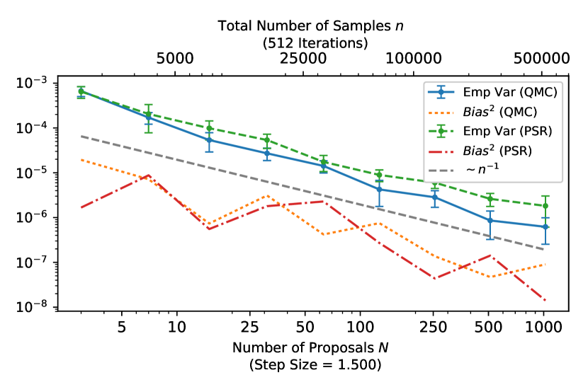
(a) Ripley, $d=3$

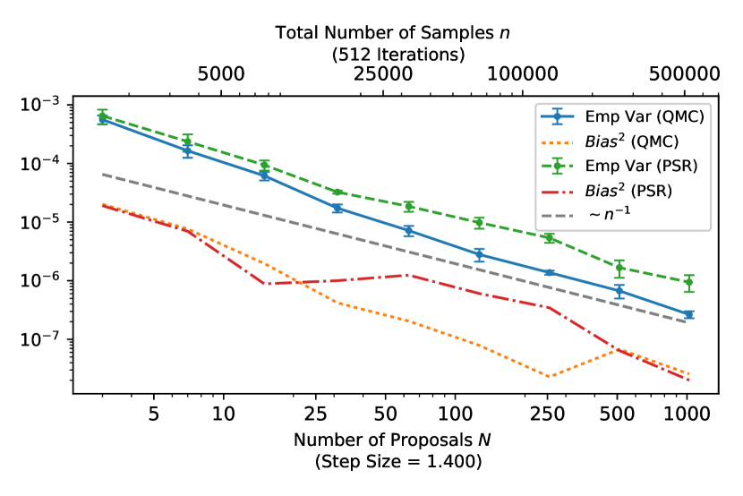
(b) Pima, $d=8$

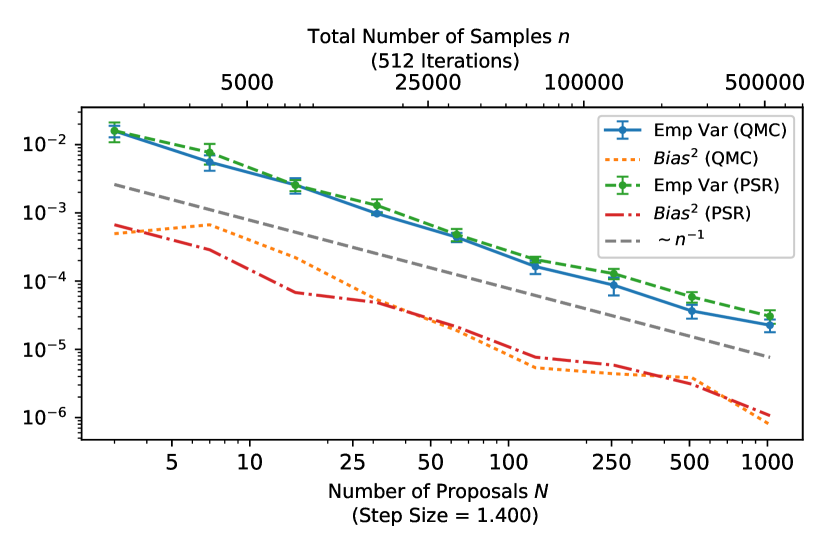
(c) Heart, $d=14$

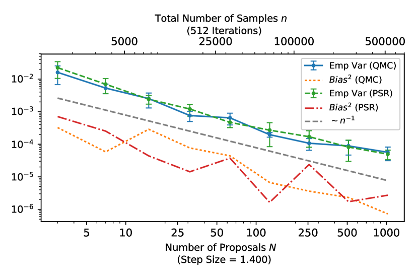
(d) Australian, $d=15$

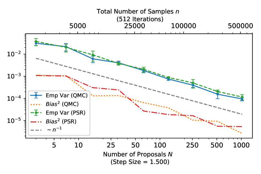
(e) German, $d=25$

Figure 9: Empirical variance and squared bias considered in an estimation associated to the Bayesian logistic regression problem from [GC11] using a pseudo-random (PSR) vs. CUD (QMC) seed, resp., for increasing proposal numbers and sample sizes. The results are based on $25$ MCMC simulations and the error bars correspond to three times a standard deviation

5.1.4 The “right” way of using CUD numbers

Due to the acceptance threshold in standard MP-MCMC, some proposals are accepted at least once while others are not accepted at all. In the latter case, the underlying QMC points that generate such proposals and that contribute to the homogeneous spatial coverage of the hypercube of QMC points are neglected. Since this homogeneity is the core of performance gain due to QMC, we do not expect the best results using CUD points when applying it to standard MP-MCMC. More successful approaches do not exhibit any discontinuity due to an acceptance threshold, e.g. Gibbs sampling [OT05, TO08]. Our approach for making use of all information carried by the underlying CUD sequence is by incorporating all proposals, which is achieved using the importance sampling approach for MP-MCMC introduced in Section 4. Indeed, as we will see in the following section, with standard MP-MCMC we achieve only a reduction in the constant associated to the rate $n^{-1}$, whereas using importance sampling there are situations where the convergence rate improves to close to $n^{-2}$.

5.2 IS-MP-QMCMC

As previously discussed in Section 5.1.4, importance sampling seems to be a solid approach in the context of MP-MCMC driven by CUD numbers, since it respects all proposals and therefore all numbers in the underlying sequence, thereby making full use of its spatial homogeneity. We now introduce IS-MP-QMCMC, prove its consistency and show an improved convergence rate compared to standard MP-MCMC or other MCMC methods in numerical experiments. The two algorithms introduced here are extensions of Algorithms 3 and 4 to using any CUD sequence as their driving sequences.

5.2.1 Algorithm description

Analogously to pseudo-random IS-MP-MCMC, introduced in Section 4, all proposals from one iteration are accepted. Thus, only a single sample of $I$ from the finite state Markov chain is generated, which determines the distribution from which the subsequent $N$ proposals are generated. The resulting method is displayed as Algorithm 6, which can be viewed as an extension of Algorithm 3 to the CUD case.

Input: Initialise starting point (proposal) $\bm{y}_{1}\in\Omega$, number of proposals $N$, auxiliary variable $I=1$, integrand $f$, initial mean estimate $\bm{\mu}_{1}=\bm{\mu}_{1}(f)$ and number of MCMC iterations $L$ ;

1 Generate a CUD sequence $u_{1},...,u_{L(Nd+1)}\in(0,1)$;

2 for each MCMC iteration $\ell=1,...,$$L$  do

3       Set $\bm{u}=(u_{(\ell-1)(Nd+M)+1},...,u_{(\ell-1)(Nd+1)+Nd})\in(0,1)^{Nd}$, and sample ${\bm{y}}_{\setminus I}$ conditioned on $I$, i.e., draw $N$ new points from $\kappa({\bm{y}}_{I},\cdot)=p({\bm{y}}_{\setminus I}|{\bm{y}}_{I})$ by the inverse $\Psi_{\bm{y}_{I}}(\bm{u})$ ;

4       Calculate the stationary distribution of $I$ conditioned on ${\bm{y}}_{1:N+1}$, i.e. $\forall$ $i=1,...,N+1$, $p(I=i|{{\bm{y}}}_{1:N+1})=$ $\pi({{\bm{y}}}_{i})\kappa({{\bm{y}}}_{{i}},{{\bm{y}}}_{\setminus{i}})/\sum_{j}\pi({{\bm{y}}}_{j})\kappa({{\bm{y}}}_{{j}},{{\bm{y}}}_{\setminus{j}})$, which can be done in parallel;

5       Compute $\tilde{\bm{\mu}}_{\ell+1}=\sum_{i}p(I=i|{{\bm{y}}}_{1:N+1})f({{\bm{y}}}_{i})$;

6       Set $\bm{\mu}_{\ell+1}=\bm{\mu}_{\ell}+\frac{1}{\ell+1}\left(\tilde{\bm{\mu}}_{\ell+1}-\bm{\mu}_{\ell}\right)$;

7       Set $v^{\prime}=u_{\ell(Nd+1)}\in(0,1]$;

8       If $v^{\prime}\in(\gamma_{j-1},\gamma_{j}]$, where $\gamma_{j}=\sum_{i=1}^{j}p(I=i|\bm{y}_{1:N+1})$ for $j=1,...,N+1$ and $\gamma_{0}:=0$, set $I=j$;

9      

10 end for

Algorithm 6 Importance sampling MP-QMCMC
We highlight all altered code compared to (pseudo-random) IS-MP-MCMC, Algorithm 3

5.2.2 Asymptotic unbiasedness of IS-MP-QMCMC

Corollary 5.5 (Asymptotic unbiasedness of IS-MP-QMCMC).

Under the conditions of Theorem 5.1, the IS-MP-QMCMC sequence of estimators $(\bm{\mu}_{L})_{L\geq 1}$ from Algorithm 6 is asymptotically unbiased.

Proof.

Due to the consistency of the underlying MP-QMCMC chain we may argue analogously to Lemma 4.1. ∎

5.2.3 Empirical results: Bayesian linear regression

Let us consider the standard linear regression problem, in which the conditional distribution of an observation $\bm{y}\in\mathbb{R}^{n}$, given a design matrix $X\in\mathbb{R}^{n\times d}$, is specified by

$$\bm{y}=X\bm{\beta}+\bm{\varepsilon},$$

where $\bm{\beta}\in\mathbb{R}^{d}$, and $\bm{\varepsilon}\sim\mathcal{N}(\bm{0},\sigma^{2}\mathbf{I}_{n})$ denotes the $n$-dimensional noise term. Each row of the matrix $X$ is a predictor vector. The resulting likelihood function is given by

$$\pi(\bm{y}|\beta,X,\sigma^{2})\propto(\sigma^{2})^{-n/2}\exp\left(-\frac{1}{2\sigma^{2}}\left(\bm{y}-X\bm{\beta}\right)^{T}\left(\bm{y}-X\bm{\beta}\right)\right).$$

In a Bayesian context, we are interested in the distribution of the weight vector $\bm{\beta}$ conditioned on the design matrix $X$, the observation $\bm{y}$, the noise variance $\sigma^{2}$ and some prior information on $\bm{\beta}$. More precisely, given the above we would like to estimate the expectation of $\bm{\beta}$. Our a priori knowledge about $\bm{\beta}$ is expressed by the prior distribution

$$\pi(\bm{\beta}|\sigma^{2})\propto|\det(\Sigma_{0})|^{-1}\exp\left(-\frac{1}{2}\bm{\beta}^{T}\Sigma_{0}^{-1}\bm{\beta}\right),$$

where $\Sigma_{0}=\sigma^{2}/g(X^{T}X)^{-1}$ with $g=1/n$. Thus, $\pi(\bm{\beta}|\sigma^{2})$ denotes Zellner’s g-prior according to [Zel86]. To estimate $\mathbb{E}_{\pi}[\bm{\beta}|\bm{y},X,\sigma^{2}]$ under the resulting posterior distribution,

$$\pi(\bm{\beta}|\bm{y},X,\sigma^{2})\propto\pi(\bm{\beta}|\sigma^{2})\pi(\bm{y}|\bm{\beta},X,\sigma^{2}),$$

the importance sampling MP-QMCMC, described in Algorithm 6, is applied. The underlying data consisting of $X$ and $\bm{y}$ is simulated according to $X\sim\mathcal{N}(\bm{0},\Sigma_{X})$ and $\bm{y}=X^{T}\bm{\beta^{*}}+\bm{\varepsilon}$, where $\bm{\beta^{*}}=(1,...,1)^{T}\in\mathbb{R}^{d}$, and $\Sigma_{X}\in\mathbb{R}^{n\times n}$ has non-negligible entries off its diagonal. Referring to Table 3, experiments are performed for dimensionalities between $d=1$ and $d=500$.

The bias of the underlying MP-MCMC methods can hereby be computed exactly as the posterior is available analytically and is given by the Gaussian $\pi(\bm{\beta}|\bm{y},X,\sigma^{2})=\mathcal{N}(\bm{\mu},\Sigma)$, where

$$\bm{\mu}=\left(X^{T}X+\Sigma_{0}\right)^{-1}\left(X^{T}X\bm{\hat{\beta}}+\Sigma_{0}\bm{\mu}_{0}\right),\quad\text{and}\quad\Sigma=\sigma\left(X^{T}X+\Sigma_{0}\right).$$

Here, $\bm{\hat{\beta}}=\left(X^{T}X\right)^{-1}X^{T}\bm{y}$ denotes the ordinary least squares solution for $\bm{\beta}$, where we made use of the Moore-Penrose pseudo-inverse for $X^{T}X$.

To generate proposals we make use of the SmMALA kernel defined in (16). Since samples from a current iteration are therefore dependent on samples from the previous iteration, the consistency of the resulting method using a CUD seed is not covered by Corollary 5.5. However, as we can see in Figure 10 and from the results for the MSE reductions given in Table 2, convergence of the MSE seems to hold true. Furthermore, using the importance sampling formulation of MP-QMCMC, together with the CUD driving sequence, results in an improved variance convergence rate of close to $n^{-2}$, compared to $n^{-1}$ when using an IID seed.

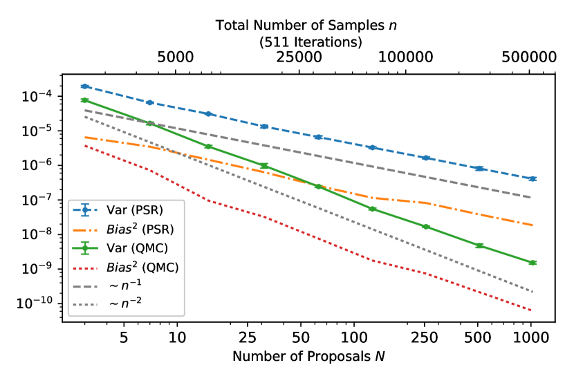
Figure 10: Empirical variance and squared bias of the sample mean in $100$-dimensional Bayesian linear regression based on IS-MP-QMCMC (SmMALA) using a pseudo-random (PSR) vs. CUD (QMC) seed, resp., for increasing proposal numbers and sample sizes. The results are based on $25$ MCMC simulations, and the error bars correspond to twice a standard deviation

Table 2: Comparison of MSE convergence rates for IS-MP-MCMC (SmMALA) using a pseudo-random (PSR) vs. a CUD (QMC) seed, resp., in Bayesian linear regression for increasing dimensionality. Displayed is also the associated reduction factor in MSE by the use of the deterministic instead of the pseudo-random seed, resp.

Dimension	MSE Rate		Reduction by using QMC
	PSR	QMC		$N=3$	$N=63$	$N=1023$
1	-1.06	-1.90		2.5	24.0	508.0
2	-1.09	-1.97		1.6	45.7	319.8
5	-1.03	-1.88		1.9	35.2	234.1
10	-1.03	-1.89		2.1	26.4	375.4
25	-1.04	-1.86		2.7	32.0	247.2
50	-1.04	-1.89		2.2	26.2	271.3
100	-1.04	-1.88		2.5	27.2	269.2
250	-1.03	-1.90		1.8	31.5	263.7
500	-1.04	-1.79		2.7	15.7	173.3

5.3 Adaptive IS-MP-QMCMC

Finally, we introduce an importance sampling method that is based on MP-QMCMC proposals with adaptation of the proposal distribution. As a result we receive Algorithm Algorithm 7, which states a direct extension of Algorithm 4 to the general CUD case.

5.3.1 Algorithm description

In every MCMC iteration, the proposal distribution is updated. More precisely, the mean and covariance of the proposal distribution, which is assumed to have a multivariate Gaussian distribution, is determined in each iteration by the average of the weighted sum mean and covariance estimates, respectively, based on previous iterations including the present one. The resulting mean estimate after the final iteration is the output of this algorithm.

Input: Initialise starting point (proposal) $\bm{y}_{1}\in\Omega$, number of proposals $N$, auxiliary variable $I=1$, integrand $f$, initial mean estimate $\bm{\mu}_{1}=\bm{\mu}_{1}(f)$, initial covariance estimate $\Sigma_{1}$ and number of MCMC iterations $L$;

1 Generate a CUD sequence $u_{1},...,u_{LNd}\in(0,1)$;

2 for each MCMC iteration $\ell=1,...,$$L$  do

3       Set $\bm{u}=(u_{(\ell-1)Nd+1},...,u_{\ell Nd})\in(0,1)^{Nd}$, and sample ${\bm{y}}_{\setminus I}$ conditioned on $I$ and $\Sigma_{\ell}$, i.e., draw $N$ new points from $\kappa_{\Sigma_{\ell}}({\bm{y}}_{I},\cdot)=p({\bm{y}}_{\setminus I}|{\bm{y}}_{I},\Sigma_{\ell})$ by the inverse $\Psi_{\bm{y}_{I}}(\bm{u}|\Sigma_{\ell})$ ;

4       Calculate the stationary distribution of $I$ conditioned on ${\bm{y}}_{1:N+1}$ and $\Sigma_{\ell}$, i.e. $\forall$ $i=1,...,N+1$, $p(I=i|{{\bm{y}}}_{1:N+1},\Sigma_{\ell})=$ $\pi({{\bm{y}}}_{i})\kappa_{\Sigma_{\ell}}({{\bm{y}}}_{{i}},{{\bm{y}}}_{\setminus{i}})/\sum_{j}\pi({{\bm{y}}}_{j})\kappa_{\Sigma_{\ell}}({{\bm{y}}}_{{j}},{{\bm{y}}}_{\setminus{j}})$, which can be done in parallel;

5       Compute $\tilde{\bm{\mu}}_{\ell+1}=\sum_{i}p(I=i|{{\bm{y}}}_{1:N+1},\Sigma_{\ell})f({{\bm{y}}}_{i})$;

6       Set $\bm{\mu}_{\ell+1}=\bm{\mu}_{\ell}+\frac{1}{\ell+1}\left(\tilde{\bm{\mu}}_{\ell+1}-\bm{\mu}_{\ell}\right)$;

7       Set $v^{\prime}=u_{\ell(Nd+1)}\in(0,1]$;

8       If $v^{\prime}\in(\gamma_{j-1},\gamma_{j}]$, where $\gamma_{j}=\sum_{i=1}^{j}p(I=i|\bm{y}_{1:N+1},\Sigma_{\ell})$ for $j=1,...,N+1$ and $\gamma_{0}:=0$, set $I=j$;

9       Compute $\tilde{{\Sigma}}_{\ell+1}=\sum_{i}p(I=i|{\bm{y}}_{1:N+1},{{\Sigma}}_{\ell})[{\bm{y}}_{i}-\bm{\mu}_{\ell+1}][{\bm{y}}_{i}-\bm{\mu}_{\ell+1}]^{T}$;

10       Set ${\Sigma}_{\ell+1}={\Sigma_{\ell}}+\frac{1}{\ell+1}(\tilde{{\Sigma}}_{\ell+1}-{\Sigma}_{\ell})$;

11      

12 end for

Algorithm 7 Adaptive importance sampling MP-QMCMC
All code altered compared to (pseudo-random) adaptive IS-MP-MCMC, Algorithm 4, is highlighted

5.3.2 Asymptotic unbiasedness of adaptive IS-MP-QMCMC

Corollary 5.6 (Asymptotic unbiasedness of adaptive IS-MP-QMCMC).

Under the conditions of Theorem 5.1, and under any of the conditions stated in Theorem 3.6, Theorem 3.8 or Theorem 3.10, the sequence of estimators $(\bm{\mu}_{L})_{L\geq 1}$ from Algorithm 7 is asymptotically unbiased.

Proof.

Consistency of the adaptive MP-QMCMC follows by the respective theorem used and Theorem 5.1. Thus, we may argue analogously to the proof of Corollary 4.2. ∎

5.4 Empirical Results: Simple Gaussian example

As a simple reference problem, we consider the estimation of the posterior mean in a generic $1$-dimensional numerical example analogously to [OT05], in which the posterior is just a standard Gaussian. For this problem, [OT05] compared the Metropolis-Hastings algorithm using a pseudo-random seed to using a QMC seed, respectively, in terms of the resulting MSEs of the estimated posterior mean. The independent sampler is given by $\mathcal{N}(0,2.4^{2})$ and the random walk sampler by $\mathcal{N}(x,2.4^{2})$, where $x\in\mathbb{R}$ denotes the last accepted sample. Here, we additionally compare those algorithms with the IS-MP-QMCMC and its adaptive version introduced in Section 5.2 and Section 5.3, respectively. In the case of the independent sampler, we apply adaptivity within AIS-MP-QMCMC not only in the proposal covariance but also in the proposal mean, according to the estimate in line 6 from Algorithm 7. For the random walk case, we do not make use of adaptivity in the mean, as the proposal sampler mean is just a sampled point from the finite state chain from one iteration. The low-discrepancy sequence used in [OT05] is based on a LCG, while the QMC construction used here is based on the LFSR introduced in [CMNO12], see Section 2.1.5 for details. Nevertheless, we receive similar results in the reduction of MSE between standard Metropolis-Hastings and its QMC-driven counterpart as [OT05] did: for the independent sampler, the MSE is reduced by a factor $\approx 7.0$, and for the random walk sampler by a factor $\approx 2.3$, respectively. In the independent sampler case, the additional performance gain using the importance sampling approaches is significant: compared to standard Metropolis-Hastings, the maximum MSE reduction is $\approx 112.2$, i.e. more than an order of magnitude (factor $\approx 16.1$) reduction compared to QMC-driven Metropolis-Hastings. Note that the performance of the multiple proposal methods increases with number of proposals used, thereby making use of less number of iterations to result in the same total number of samples. In the case of random walk proposals, the additional gain is less substantial. Compared to standard Metropolis-Hastings we receive a maximum MSE reduction of $\approx 6.3$, i.e. a decrease of $\approx 2.7$ compared to QMC-driven Metropolis-Hastings.

Table 3: Comparison of standard Metropolis-Hastings with different QMC driven MCMC algorithms for independent and random walk proposals on a 1-dimensional Gaussian numerical example with $65535$ samples. The numbers in the brackets correspond to three-times a standard deviation

Method	Independence		Random Walk
	Mean	MSE		Mean	MSE
PSR Metropolis-Hastings	$-1.64\times 10^{-4}$	$3.60\times 10^{-5}(\pm 6.96\times 10^{-6})$		$-8.76\times 10^{-5}$	$6.76\times 10^{-5}(\pm 6.56\times 10^{-6})$
QMC Metropolis-Hastings	$1.96\times 10^{-4}$	$5.17\times 10^{-6}(\pm 1.61\times 10^{-6})$		$1.17\times 10^{-4}$	$2.88\times 10^{-5}(\pm 6.68\times 10^{-6})$
IS-MP-QMCMC (4)	$-1.97\times 10^{-4}$	$3.56\times 10^{-6}(\pm 3.56\times 10^{-7})$		$-1.20\times 10^{-3}$	$2.74\times 10^{-5}(\pm 7.70\times 10^{-6})$
Adapt. IS-MP-QMCMC (4)	$-1.64\times 10^{-4}$	$4.31\times 10^{-6}(\pm 2.94\times 10^{-7})$		$-1.44\times 10^{-3}$	$2.81\times 10^{-5}(\pm 8.11\times 10^{-6})$
IS-MP-QMCMC (32)	$-2.10\times 10^{-5}$	$7.72\times 10^{-7}(\pm 1.53\times 10^{-7})$		$-2.63\times 10^{-4}$	$1.07\times 10^{-5}(\pm 1.52\times 10^{-6})$
Adapt. IS-MP-QMCMC (32)	$-1.15\times 10^{-4}$	$7.83\times 10^{-7}(\pm 1.60\times 10^{-7})$		$-5.62\times 10^{-4}$	$1.26\times 10^{-5}(\pm 1.44\times 10^{-6})$
IS-MP-QMCMC (256)	$9.44\times 10^{-5}$	$5.32\times 10^{-7}(\pm 1.29\times 10^{-7})$		$-4.39\times 10^{-4}$	$1.21\times 10^{-5}(\pm 2.78\times 10^{-6})$
Adapt. IS-MP-QMCMC (256)	$-1.29\times 10^{-5}$	$3.21\times 10^{-7}(\pm 6.17\times 10^{-8})$		$-3.29\times 10^{-4}$	$1.07\times 10^{-5}(\pm 1.35\times 10^{-6})$

5.5 Empirical Results: Bayesian logistic regression

We now apply the proposed adaptive important sampling method as described in Algorithm 7 to the Bayesian logistic regression from Section 4.4. As proposal sampler, we apply a Gaussian kernel that samples independently of previous samples and adaptively updates its mean and covariance according to the weighted estimates from Algorithm 7, respectively. Note that no gradient information about the posterior is needed in this case. We compare the performance of the respective QMC algorithm to its pseudo-random version in terms of the empirical variance of their posterior mean estimates. As a reference, we perform the same experiments also for standard Metropolis-Hastings and SmMALA Metropolis-Hastings. Thereby, we employ the same total number of samples $n$ as the respective multiple proposal algorithms produce, i.e. $n=LN$, where $L$ denotes the number of iterations and $N$ the number of proposals used. This guarantees a fair comparison between the single and multiple proposal algorithms. The results for the datasets of varying dimension and increasing proposal numbers (total number of samples) are displayed in Figure 11. Again, we observe an improved convergence rate in the empirical variance of our estimator, which in many cases is close to $n^{-2}$. Further, Table 4 displays the associated reductions in empirical variance between the adaptive IS-MP-QMCMC and the other algorithms. Due to the improved convergence, the reductions increase with increasing proposal numbers and thus total numbers of proposals, leading to significant reductions in all models and compared to all algorithms for a large number of proposals. In some situations, a reduction of more than $4$ orders of magnitude compared to standard Metropolis-Hastings can be observed, and more than $2$ orders of magnitude compared to the SmMALA Metropolis-Hastings as well as compared to pseudo-random IS-MP-MCMC. For any model and throughout all number of proposals employed, the reduction compared to the two reference algorithms is significant.

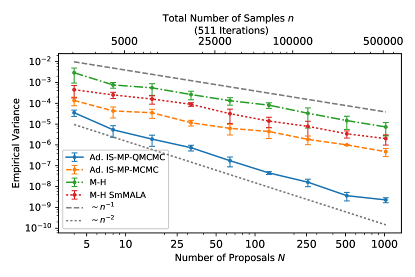
(a) Ripley, $d=3$

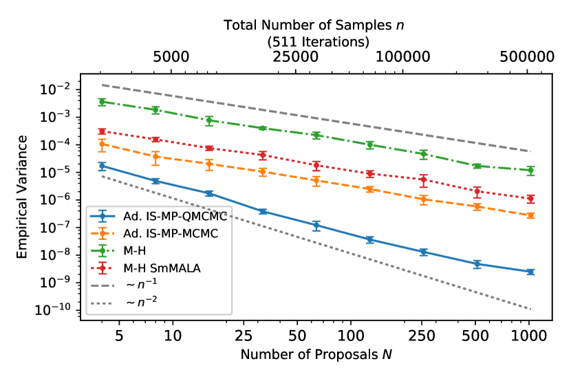
(b) Pima, $d=8$

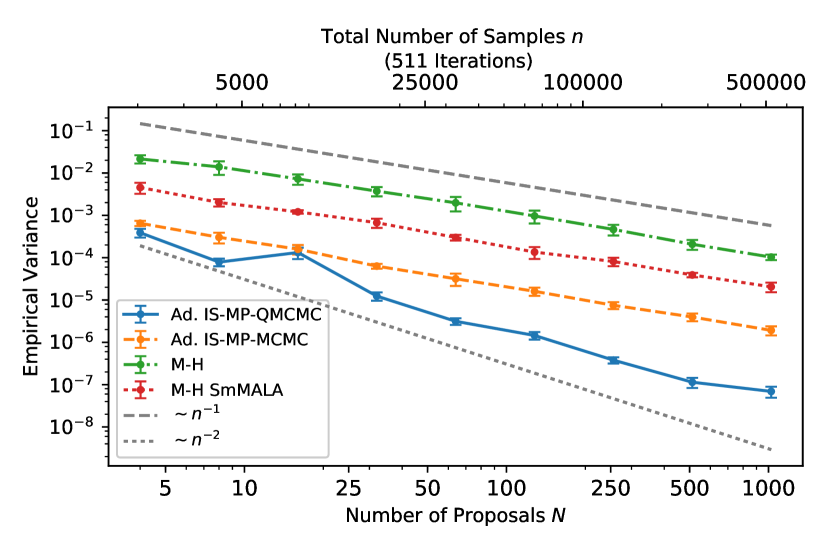
(c) Heart, $d=14$

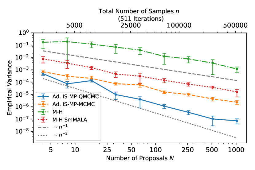
(d) Australian, $d=15$

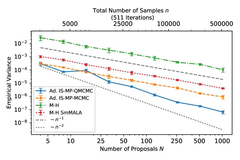
(e) German, $d=25$

Figure 11: Empirical variance of adaptive IS-MP-QMCMC compared to adaptive IS-MP-MCMC, SmMALA Metropolis-Hastings (M-H SmMALA) and standard Metropolis-Hastings (M-H), resp., for the Bayesian logistic regression problem from 4.4. Here, M-H SmMALA was tuned to an approximately optimal acceptance rate of $50$-$60\%$, and M-H to $20$-$25\%$. For the adaptive methods, a Burn-In of between 0-8192 samples, increasing with dimensionality $d$, was discarded. The results are based on $25$ MCMC simulations and the errors bands correspond to three times a standard deviation

Table 4: Ratio of empirical variances of adaptive IS-MP-QMCMC compared to adaptive IS-MP-MCMC, SmMALA Metropolis-Hastings (M-H SmMALA) and standard Metropolis-Hastings (M-H), resp., for the Bayesian logistic regression problem from 4.4. Here, M-H SmMALA was tuned to an approximately optimal acceptance rate of $50$-$60\%$, and M-H to $20$-$25\%$. The results are based on $25$ MCMC simulations

	Ad. IS-MP-QMCMC	Ratio in empirical variance for $N=$
	VS		$4$	$8$	$16$	$32$	$64$	$128$	$256$	$512$	$1024$
	Ad. IS-MP-MCMC		$3.9$	$8.1$	$18.5$	$15.8$	$35.7$	$97.7$	$113.5$	$274.7$	$207.1$
Ripley	M-H SmMALA		$12.7$	$47.5$	$84.0$	$121.0$	$179.9$	$309.7$	$479.4$	$933.2$	$880.7$
	M-H		$82.8$	$142.8$	$290.8$	$356.8$	$759.3$	$1794.6$	$2040.6$	$4040.5$	$3191.7$
	Ad. IS-MP-MCMC		$6.2$	$7.6$	$11.7$	$27.5$	$41.7$	$67.6$	$81.1$	$120.2$	$110.3$
Pima	M-H SmMALA		$18.1$	$32.0$	$43.7$	$110.8$	$148.5$	$244.7$	$422.7$	$430.8$	$448.9$
	M-H		$211.3$	$378.5$	$445.3$	$1038.2$	$1837.7$	$2739.3$	$3561.0$	$3568.3$	$4808.5$
	Ad. IS-MP-MCMC		$1.6$	$3.9$	$1.2$	$5.1$	$10.1$	$11.0$	$19.8$	$34.7$	$27.7$
Heart	M-H SmMALA		$11.7$	$25.6$	$9.1$	$54.2$	$95.8$	$93.2$	$213.9$	$342.0$	$296.1$
	M-H		$55.2$	$177.7$	$54.8$	$301.7$	$629.2$	$665.3$	$1225.1$	$1815.6$	$1486.8$
	Ad. IS-MP-MCMC		$1.4$	$4.1$	$1.5$	$7.5$	$15.2$	$13.9$	$28.2$	$42.1$	$32.8$
Australian	M-H SmMALA		$15.9$	$46.7$	$11.4$	$46.6$	$76.0$	$125.1$	$193.7$	$367.5$	$222.5$
	M-H		$359.6$	$2664.2$	$917.4$	$7017.4$	$9842.3$	$10985.6$	$21625.8$	$34043.2$	$16010.5$
	Ad. IS-MP-MCMC		$1.0$	$2.2$	$0.8$	$2.6$	$3.1$	$6.1$	$12.2$	$9.4$	$14.0$
German	M-H SmMALA		$3.4$	$8.1$	$2.8$	$10.0$	$11.2$	$26.5$	$48.3$	$46.5$	$62.6$
	M-H		$92.1$	$195.0$	$64.8$	$255.7$	$301.0$	$622.9$	$1076.5$	$1465.6$	$1595.2$

5.6 Empirical Results: Bayesian inference in non-linear differential equations

An important category of inverse problems concern the study of uncertainty quantification in dynamical systems given by a set of ordinary differential equations (ODEs). Typically, such a system can be formalised by $M$ coupled ODEs and a model parameter $\bm{\theta}\in\mathbb{R}^{d}$, which describes the dynamics of the system’s state $\bm{x}\in\mathbb{R}^{M}$ in terms of its time derivative by $\mathrm{d}\bm{x}/\mathrm{d}t=\bm{f}(\bm{x},\bm{\theta},t)$. Given state observations $\bm{y}(t)$ at $T$ distinct points in time, our aim is to infer about the underlying parameter $\bm{\theta}$ and, more specifically, about integral quantities $\int g(\bm{\theta})\mathrm{d}\bm{\theta}$ for an integrable scalar-valued function $g$. An observation $\bm{y}(t)$ at time $t$ is usually subject to a measurement error, which can be modeled as $\bm{y}(t)=\bm{x}(t)+\bm{\varepsilon}(t)$, where $\bm{\varepsilon}(t)\in\mathbb{R}^{M}$ states a suitable multivariate noise variate at time $t$. Often, $\bm{\varepsilon}(t)$ is Gaussian with zero mean and standard deviation $\sigma_{m}$ in the $n$th component for $m=1,...,M$. Given $T$ distinct observations, the observed system can be summarised in matrix notation by $Y=X+E$, where $Y,X,E$ denote $T\times M$ matrices whose rows correspond to the observation process at the distinct $T$ points in time. To generate a sample $X$ one needs to solve the underlying set of ODEs given the model parameter $\bm{\theta}$ and an initial condition $\bm{x}_{0}$, i.e. $X=X(\bm{\theta},\bm{x}_{0})$. If $\pi(\bm{\theta})$ denotes the prior for $\bm{\theta}$, the posterior density of $\bm{\theta}|Y$ can then be expressed as

$$\pi(\bm{\theta}|Y)\propto\pi(\bm{\theta})\prod_{m}\mathcal{M}\left(Y_{1:T,m}|X(\bm{\theta},\bm{x}_{0})_{1:T,m},\Sigma_{n}\right).$$ (31)

In the following, experiments based on the adaptive importance sampling QMCMC scheme for multiple proposals introduced in Section 5.3 are performed for two different ODE models, namely the Lotka-Volterra and the FitzHugh-Nagumo model.

5.6.1 Lotka-Volterra

The Lotka-Volterra equations are a set of two non-linear ODEs that describe the interaction between two species in a predator-prey relationship. Formally, this can be expressed as

$$\frac{\mathrm{d}u}{\mathrm{d}t} =\alpha u-\beta uv$$ (32)

$$\frac{\mathrm{d}v}{\mathrm{d}t} =\gamma uv-\delta v,$$ (33)

where $u$ and $v$ represent the population of prey and predators, respectively, and $\alpha,\beta,\gamma,\delta>0$ determine the interaction between the two species given $\mathrm{d}u/\mathrm{d}t$ and $\mathrm{d}v/\mathrm{d}t$.

We used 400 data points generated by the respective models between $t\in[0,8]$. The respective model parameters were chosen as $\alpha=1.8,\beta=0.5,\gamma=2.5$ and $\delta=1$, and the initial conditions as $u(0)=10$ and $v(0)=5$. To the model state outcomes was then added a Gaussian noise with standard deviation equal to $0.25$. In Figure 12, the underlying true state trajectories together with their noisy measurements are displayed.

5.6.2 FitzHugh–Nagumo

The FitzHugh-Nagumo model is a set of two non-linear ODEs that describe the dynamics of an excitable system in terms of two states, namely a membrane voltage $u$ and a recovery variable $v$, defined by

$$\frac{\mathrm{d}u}{\mathrm{d}t} =\gamma\left(u-\frac{u^{3}}{3}+v\right)$$ (34)

$$\frac{\mathrm{d}v}{\mathrm{d}t} =-\left(\frac{u-\alpha+\beta v}{\gamma}\right).$$ (35)

Here, $\alpha,\beta$ and $\gamma$ serve as scaling parameters and to determine the unstable equilibrium state value.

The underlying data consists of 200 data points produced by the FitzHugh-Nagumo model between $t\in[0,2]$ with model parameters $\alpha=0.5,\beta=0.5,\gamma=1.5$ and initial conditions $u(0)=-1$ and $v(0)=1$. A Gaussian noise with standard deviation $1$ was then added to the model outcomes. Figure 12 (b) shows the model outcomes and the associated noisy observations.

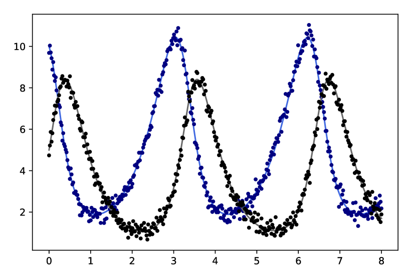
(a) Lotka-Volterra

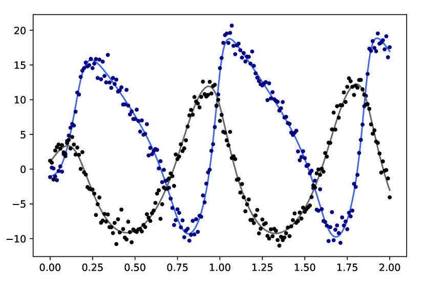
(b) FitzHugh-Nagumo

Figure 12: Output for both states $u$ and $v$ in (a) the Lotka-Volterra model with parameters $\alpha=1.8,\beta=0.5,\gamma=2.5$ and $\delta=1$, and in (b) the FitzHugh-Nagumo model with parameters $\alpha=0.5,\beta=0.5$ and $\gamma=1.5$, respectively; the dots correspond to the respective noisy data

5.6.3 Numerical results

The performance of using QMC numbers compared to using pseudo-random numbers as driving sequence is investigated numerically for the adaptive IS-MP-MCMC algorithm. As a reference, the respective simulations are also performed for a random-walk Metropolis-Hastings within Gibbs algorithm, which corresponds to performing a Metropolis-Hastings step within each directional component update in a Gibbs sampler. The standard Metropolis-Hastings algorithm suffers severely from low mixing for the considered problems, and therefore did not qualify as a performance reference. To satisfy fairness of comparison, the Metropolis-Hastings within Gibbs algorithm produces the same number $n$ of total samples as the multiple proposal algorithms, i.e. $n=LN$ with $L$ denoting the number of iterations and $N$ the number of proposals.

Non-linear ODEs generally produce corresponding non-linear features in the posterior distribution, which can result in the emergence of multiple local maxima. It is therefore germane to ensure for an underlying MCMC method not to dwell in a wrong mode. However, to allow for the comparison of sampling efficiency measured by the empirical variance of estimates, we employ the respective MCMC methods initialised on the true mode. As initial proposal mean and covariance in the adaptive IS-MP-MCMC algorithms a rough posterior mean and covariance estimate was used. The former further served as initial value for the Metropolis-Hastings within Gibbs algorithm, whose steps sizes for individual components was chosen to meet an acceptance rate between $20$-$40\%$.

The outcomes of the numerical experiments associated to the inference problems for the ODE models introduced above are shown in Figure 13 and Table 5. As a prior, a Gamma distribution with shape parameter equal to $1$ and scale parameter equal to $3$, truncated at zero, was employed in both model problems. A clear improvement in the rate of convergence, being close to $n^{-2}$ in both the Lotka-Volterra and the FitzHugh-Nagumo case can be observed. In addition, we observe significant reductions in empirical variance for increasing numbers of proposals for adaptive IS-MP-QMCMC compared to its pseudo-random version and the reference Metropolis-Hastings within Gibbs algorithm. Compared to the latter, a maximal reduction of over $6$ orders of magnitude could be achieved.

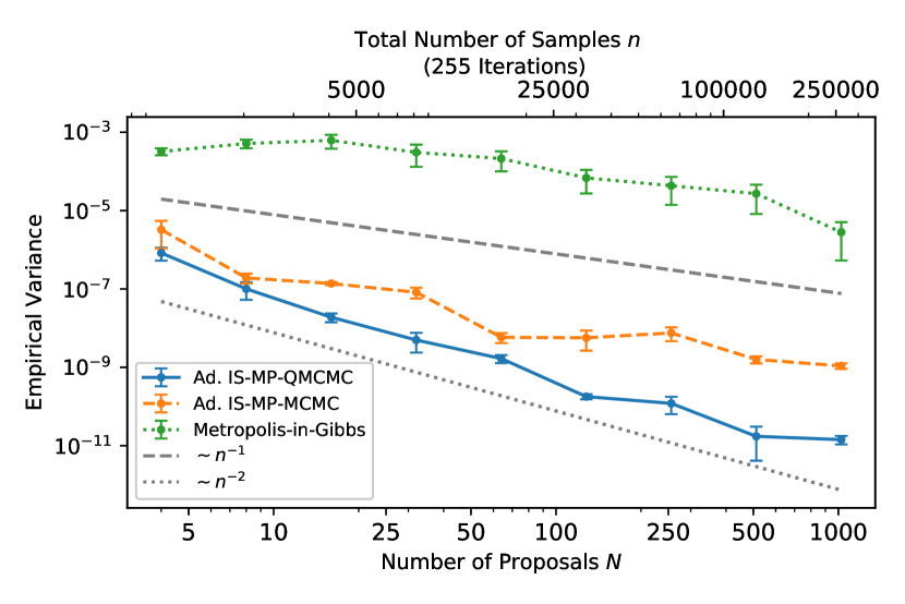
(a) Lotka-Volterra

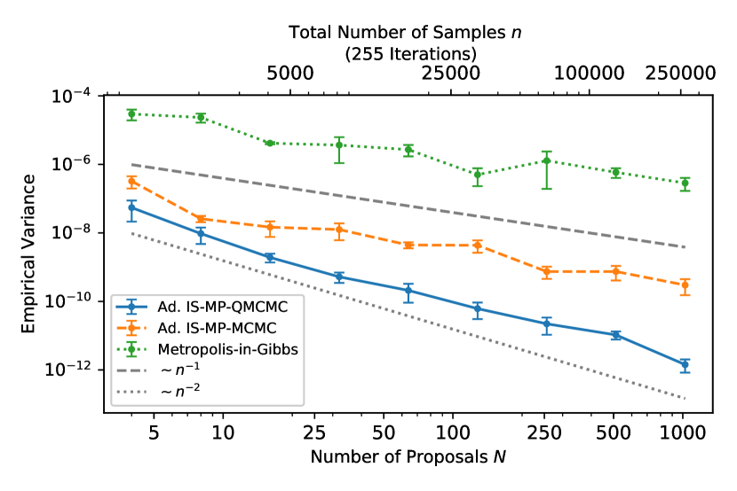
(b) FitzHugh-Nagumo

Figure 13: Empirical variance of the posterior mean estimate associated to the (a) Lotka-Volterra and (b) FitzHugh-Nagumo model inference problem, using a pseudo-random (PSR) vs. CUD (QMC) seed, resp., for increasing proposal numbers and sample sizes; also displayed are the results for the random-walk Metropolis-Hastings within Gibbs as a reference, tuned to an acceptance rate between $20$-$40\%$. The results are based on $10$ MCMC simulations. The error band correspond to twice a standard deviation

Table 5: Ratio of empirical variances of adaptive IS-MP-QMCMC compared to adaptive IS-MP-MCMC and random-walk Metropolis-Hastings within Gibbs (M-H in Gibbs), resp., for the ODE model inference problems from 5.6.1 and 5.6.2, respectively. Here, Metropolis-Hasting within Gibbs was tuned to an acceptance rate between $20$-$40\%$. The results are based on $10$ MCMC simulations

	Ad. IS-MP-QMCMC	Ratio in empirical variance for $N=$
	VS		$4$	$8$	$16$	$32$	$64$	$128$	$256$	$512$	$1024$
Lotka-Volterra	Ad. IS-MP-MCMC		$3.9$	$1.9$	$7.3$	$16.5$	$3.5$	$31.6$	$62.7$	$91.5$	$76.2$
	M-H in Gibbs		$389.3$	$5129.5$	$32677.7$	$61495.1$	$127050.1$	$381491.6$	$358768.2$	$1559126.1$	$196450.0$
FitzHugh-Nagumo	Ad. IS-MP-MCMC		$5.9$	$2.7$	$7.6$	$24.0$	$21.1$	$70.5$	$33.5$	$70.9$	$209.6$
	M-H in Gibbs		$540.3$	$2455.1$	$2160.8$	$7005.2$	$12887.9$	$8128.5$	$57942.5$	$55702.0$	$199902.3$

5.7 Intuition for increased convergence using importance sampling and QMC combined

Vanilla MP-MCMC has, independently of the underlying driving sequence, an acceptance mechanism that works similarly to classical Metropolis-Hastings: some proposals are accepted while others are refused, according to some acceptance ratio. This procedure can be viewed as introducing a discontinuity in the mapping between seed and actual samples. This can be explained more precisely as follows. Every proposal of dimensionality $d$ is generated based on a tupel of size $d$ from the underlying driving sequence. If the driving sequence is QMC, then it is homogeneously distributed on the unit interval. To refuse a proposal means to discard the underlying tupel from the driving sequence that created it. However, discarding points means figuratively speaking creating holes in the otherwise equidistributed point set, which damages its homogeneity. Since this homogeneity is the core of performance gain brought by QMC we cannot expect vanilla MP-QMCMC to converge at a faster rate. In contrast to this, in the extension to importance sampling every proposal is accepted and weighted such that the entire underlying seed is respected. Therefore the previously mentioned discontinuity is removed. Convergence rates close to $n^{-2}$ known from vanilla QMC are then possible as our numerical experiments illustrate.

5.8 Pros and Cons of using CUD numbers in MCMC

Whenever the regularity conditions formulated in Section 3.2 are satisfied, consistency of the resulting MCMC algorithm is guaranteed. However, in applications where these do not hold true, e.g. in the algorithm used in 5.2.3, numerical experiments suggest that the resulting samples asymptotically still follow the target distribution. In none of the experiments that we performed the CUD version of MP-MCMC along with its extensions (importance sampling, MALA, nonreversible kernels, etc.) has performed significantly worse than standard MCMC using a pseudo-random seed. However, in many simulations the benefit of using CUD numbers as driving sequence compared to IID numbers is substantial, see Sections 5.2.3, 5.4, 5.5 and 5.6.

The downside of using CUD numbers is that one relies on a construction that must first be developed, implemented and computed previous to running any MCMC experiments. The implementation might become expensive when the number of required samples is large. However, once a finite sequence is constructed, it can be reused for as many applications and experiments as one requires. Further, many CUD constructions do not allow a user-defined specific length of the sequence, but rather certain unique lengths. For example, some CUD constructions correspond to PRNGs with a short period $p$. In the case of this work, an LFSR construction was used which has a period of $p=2^{s}-1$ for $s\in\mathbb{N}$. Thus, sample sizes that differ by roughly a factor of two can be achieved, which limits the general applicability in the case of user-defined sample sizes.

6 Discussion and Conclusions

There is a rich history of research in QMC, importance sampling and MCMC methods, however these have tended to take different paths and have developed into somewhat separate research communities. This paper adds to the growing literature that ties together these complementary directions, and provides a demonstration that combining these ideas can result in computationally efficient and practically useful methodology, which we hope will prompt much more research into the intersection of these Monte Carlo techniques.

6.1 Contributions

We have significantly built upon a recent generalisation of Metropolis-Hastings, which allows for straight-forward parallelisation of MCMC by making multiple proposals at each iteration, and we have proposed numerous methodological extensions and proven some fundamental theoretical results. In particular, we investigated the use of non-reversible and optimised transition kernels within the proposal sub-sampling step of this method, and compared the relative performance of these approaches through a simulation study. We then extended this basic algorithm to make use of adaptivity of the proposal kernel and importance sampling, which can be considered as the limiting case of sampling from the finite state Markov chain on the multiple proposals. In addition, for the seven proposed algorithms, we have proven a variety of theoretical results, including limit theorems, asymptotic unbiasedness of the proposed importance sampling based estimators and ergodicity of the proposed adaptive samplers.

We then showed how this general framework offers a principled and effective way of incorporating CUD numbers from the quasi-Monte Carlo literature into Markov chain Monte Carlo. In the case of using a driving sequence of CUD numbers, we prove consistency and asymptotic unbiasedness of our method under suitable regularity conditions. Furthermore, we demonstrated that the use of importance sampling based estimators together with CUD numbers results in an MCMC method, whose mean square error empirically converges at a rate closer to $n^{-2}$ rather than the standard ${n^{-1}}$ of pseudo-randomly driven MCMC algorithms. We argue that importance sampling removes the discontinuity induced by the acceptance threshold inherent in standard Metropolis-Hastings, thereby incorporating all points from the underlying homogeneously distributed CUD driving sequence. This leads to a smaller discrepancy, which is generally the basis of an increased performance when using QMC over pseudo-random numbers.

6.2 Further research directions

The work we have presented in this paper offers many interesting and potentially very useful theoretical, methodological and practical avenues for further research that tie together ideas from the MCMC and QMC literature.

We have provided strong numerical evidence of the increased convergence rates that are possible by incorporating CUD numbers within a highly parallelisable multiple proposal MCMC algorithm, and so a natural question is whether theoretical results on the convergence rate for IS-MP-QMCMC are possible? While it appears to be a very challenging problem to tackle theoretically, some initial results on the convergence rate of CUD driven MCMC are given in [Che11], which may potentially be extended. The proofs we derive in this paper depend on the existence of a coupling region, which exists for an independent sampler, as well as asymptotically when incorporating adaptivity. Empirical results suggest that this should also hold for dependent proposals, however a coupling region does not appear to be available for such an argument. Further research could therefore investigate whether there exists a consistency proof that does not rely on the coupling region condition, perhaps based on the contraction condition in [CDO⁺11] instead.

From a methodological perspective, there are many ways in which our work could be extended, for example investigating the use of variational approximations as proposal distributions, or indeed the use of optimal transport approximations for highly non-Gaussian target densities. With the advent of RKHS and low-discrepancy sequences tailored to the underlying integrand, more challenging integration problems in very high-dimensional spaces can be more efficiently solved using QMC, circumventing the curse of dimensionality. In light of this development, the use of QMC in MCMC becomes significantly more relevant, and this link is worthy of further investigation. Furthermore, in this work we have used one particular construction of CUD numbers, although there is much research currently taking place in this area. Could other constructions perhaps offer even greater efficiency gains within the proposed framework?

Finally, there are many practical avenues of the above suggestions for research, including investigation of this methodology across a wider range of statistical models, experimental comparisons of different CUD constructions, and eventually the development of robust implementations in software to allow a wider range of practitioners to benefit more easily from the increased convergence rates and parallelisation offered by these multiple proposal quasi-Markov chain Monte Carlo methods.

Appendix A Transition kernel derivation, Section 3.1

Here, we derive the equations from Section 3.1.2 and Section 3.1.4 for the transition probabilities based on the formulation of the Markov chain defined on the product space of proposals and auxiliary variables per iteration, and on the space of accepted variables per iteration, respectively, in detail. We thereby make use of the same notation as in the respective sections above.

A.1 Derivation in Section 3.1.2

A more thorough derivation of equation (8), using the notation from Section 3.1.2 is,

$$\hat{P}(\tilde{z},z) =\hat{P}((\tilde{\bm{y}}_{1:N+1},\tilde{I}_{1:M}=\tilde{i}_{1:M}),(\bm{y}_{1:N+1},I_{1:M}=i_{1:M}))$$

$$=\kappa(\tilde{\bm{y}}_{\tilde{i}_{M}},\bm{y}_{\setminus{i_{M}}})p(I_{1:M}=i_{1:M}|\bm{y}_{1:N+1},\tilde{I}_{M}=\tilde{i}_{M})$$

$$=\kappa(\bm{y}_{i_{0}},\bm{y}_{\setminus{i_{0}}})\prod_{m=1}^{M}p(I_{m}=i_{m}|\bm{y}_{1:N+1},I_{m-1}=i_{m-1})$$

$$=\kappa(\bm{y}_{i_{0}},\bm{y}_{\setminus{i_{0}}})\prod_{m=1}^{M}A(i_{m-1},{i_{m}}),$$

where we used that $\tilde{i}_{M}=i_{0}$ and $\tilde{\bm{y}}_{\tilde{i}_{M}}=\bm{y}_{i_{0}}$. If the latter is not assumed, we need to add the term $\delta_{\tilde{\bm{y}}_{\tilde{i}_{M}}}(\bm{y}_{i_{0}})$ to the expression of the transition kernel. Equation (9) then follows in detail, as

$$\hat{P}(\tilde{z},B) =\hat{P}((\tilde{\bm{y}}_{1:N+1},\tilde{I}_{1:M}=\tilde{i}_{1:M}),C_{1:{N+1}}\times D_{1:M})$$

$$=\int_{C_{1:N+1}}\kappa(\bm{y}_{i_{0}},\bm{y}_{\setminus{i_{0}}})\delta_{\tilde{\bm{y}}_{\tilde{i}_{M}}}(\bm{y}_{i_{0}})\sum_{i_{1:M}\in D_{1:M}}\prod_{m=1}^{M}A(i_{m-1},i_{m})\mathrm{d}\bm{y}_{1:N+1}$$

$$=\chi_{C_{i_{0}}(\tilde{\bm{y}}_{\tilde{i}_{M}})}\int_{C_{\setminus{i_{0}}}}\kappa(\bm{y}_{i_{0}}=\tilde{\bm{y}}_{\tilde{i}_{M}},\bm{y}_{\setminus{i_{0}}})\sum_{i_{1:M}\in D_{1:M}}\prod_{m=1}^{M}A(i_{m-1},i_{m}|\bm{y}_{i_{0}}=\tilde{\bm{y}}_{\tilde{i}_{M}})\mathrm{d}\bm{y}_{\setminus{i_{0}}},$$

where we used the same notation as in Section 3.1.2.

A.2 Transition kernel derivation, Section 3.1.4

In order to derive equation (10) in more detail, we consider the relationship between the transition kernel $\hat{P}$ on the product space of proposals and auxiliary variables and the transition kernel $P$ on the space of accepted samples more thoroughly. First, let us treat the case of $M=N=1$, which corresponds to standard Metropolis-Hastings. Based on the current sample $\tilde{\bm{x}}$, or in terms of $\hat{P}$ any state $(\tilde{\bm{y}}_{1:2},\tilde{I}=\tilde{i})$ with $\tilde{\bm{y}}_{\tilde{i}}=\tilde{\bm{x}}$, for the next accepted sample it holds $\bm{x}\in B\in\mathcal{B}(\Omega)$, either if $\tilde{\bm{x}}\in B$ and the additional proposal is refused or the additional proposal is $\in B$ and is moreover accepted, i.e.

$$P(\tilde{\bm{x}},B) =\chi_{B}(\tilde{\bm{x}})\int_{\mathbb{R}^{d}}\kappa(\bm{y}_{i_{0}}=\tilde{\bm{x}},\bm{y}_{\setminus{i_{0}}})\left[1-A(i_{0},{\setminus{i_{0}}}|\bm{y}_{i_{0}}=\tilde{\bm{x}})\right]\mathrm{d}\bm{y}_{\setminus{i_{0}}}$$

$$\quad+\int_{B}\kappa(\bm{y}_{i_{0}}=\tilde{\bm{x}},\bm{y}_{\setminus{i_{0}}})A(i_{0},{\setminus{i_{0}}}|\bm{y}_{i_{0}}=\tilde{\bm{x}})\mathrm{d}\bm{y}_{\setminus{i_{0}}}$$

$$=\int_{B}\int_{\mathbb{R}^{d}}\delta_{\tilde{\bm{x}}}(\bm{y}_{i_{0}})\kappa(\bm{y}_{i_{0}},\bm{y}_{\setminus{i_{0}}})\left[1-A(i_{0},{\setminus{i_{0}}})\right]\mathrm{d}\bm{y}_{\setminus{i_{0}}}\mathrm{d}\bm{y}_{i_{0}}$$

$$\quad+\int_{\mathbb{R}^{d}}\int_{B}\delta_{\tilde{\bm{x}}}(\bm{y}_{i_{0}})\kappa(\bm{y}_{i_{0}},\bm{y}_{\setminus{i_{0}}})A({i_{0}},{\setminus{i_{0}}})\mathrm{d}\bm{y}_{\setminus{i_{0}}}\mathrm{d}\bm{y}_{i_{0}}$$

$$=\hat{P}\left(\tilde{\bm{x}},\left[B\times\mathbb{R}^{d}\times\{i_{0}\}\right]\ \cup\ \left[\mathbb{R}^{d}\times B\times\{\setminus i_{0}\}\right]\right).$$

The case $M=1$, and general $N\in\mathbb{N}$, can be treated in a similar fashion. In order to have $\bm{x}\in B\in\mathcal{B}(\Omega)$, either $\tilde{\bm{x}}\in B$ and all $N$ additional proposals are refused, or one of the additional proposals is $\in B$ and is moreover accepted, the latter case factorising into $N$ separate cases:

$${P}(\tilde{\bm{x}},B) =\chi_{B}(\tilde{\bm{x}})\int_{\Omega^{N}}\kappa(\bm{y}_{i_{0}}=\tilde{\bm{x}},\bm{y}_{\setminus{i_{0}}})\bigg{[}1-\sum_{i\neq i_{0}}A(i_{0},i|\bm{y}_{i_{0}}=\tilde{\bm{x}})\bigg{]}\mathrm{d}\bm{y}_{\setminus{i_{0}}}$$

$$\quad+\sum_{i=1}^{N}\int_{\Omega^{(i-1)d}\times B\times\Omega^{(N-i)d}}\kappa(\bm{y}_{i_{0}}=\tilde{\bm{x}},\bm{y}_{\setminus{i_{0}}})A(i_{0},i|\bm{y}_{i_{0}}=\tilde{\bm{x}})\mathrm{d}\bm{y}_{\setminus{i_{0}}}$$

$$=\sum_{i=1}^{N+1}\int_{\Omega^{(i-1)d}\times B\times\Omega^{(N+1-i)d}}\delta_{\tilde{\bm{x}}}(\bm{y}_{i_{0}})\kappa(\bm{y}_{i_{0}},\bm{y}_{\setminus{i_{0}}})A(i_{0},i)\mathrm{d}\bm{y}_{1:N+1}$$

$$=\hat{P}\bigg{(}\tilde{\bm{x}},\bigcup_{i=1}^{N+1}\left[\Omega^{(i-1)d}\times B\times\Omega^{(N+1-i)d}\times\{i\}\right]\bigg{)},$$

The general case of $M,N\in\mathbb{N}$, corresponding to equation (10) now follows from carefully considering what composition of sets allow for $\bm{x}_{1:M}\in B\in\Omega^{M}\subset\mathbb{R}^{Md}$.

Appendix B Proof of MP-MCMC limit theorems, Section 3.6

We now prove the law of large numbers and the central limit theorem for MP-MCMC.

B.1 Proof of Lemma 3.1, LLN for MP-MCMC

Proof.

It was proven that the Markov chain on the product space on variables $(\bm{y}_{1:N+1},I)$ has an invariant distribution that is preserved by the updating kernel due to detailed balance. According to 3.1.3, the same chain can be described on the accepted samples $\bm{x}_{1:M}\in\Omega^{M}$ in one iteration or on the product space of proposals and auxiliary variables $(\bm{y}_{1:N+1},I_{1:M})\in\Omega^{N+1}\times\{1,...,N+1\}^{M}$ in one iteration. The resulting stationary distribution on any of the respective spaces, we denote for simplicity by $p$. We apply Theorem 17.0.1 and Theorem 17.1.6 from [MT12], which state that for any scalar-valued, integrable function $F$ on $\mathbb{R}^{Md}$ it holds $\hat{\mu}_{F,n}\rightarrow\mu_{F}$ a.s., where

$$\hat{\mu}_{F,n} =\frac{1}{n}\sum_{\ell=1}^{n}F(\bm{x}_{1:M}^{(\ell)}),\text{ and},$$

$$\mu_{F} =\mathbb{E}_{p}\left[F(\bm{x}_{1:M})\right].$$

Let us define

$$F(\bm{x}_{1:M})=\frac{1}{M}\sum_{m=1}^{M}f(\bm{x}_{m}).$$

Thus, $\hat{\mu}_{F,n}=\hat{\mu}_{n,M,N}$, as defined in (17). Further, note that $\bm{x}_{m}^{(\ell)}=\bm{y}_{I_{m}^{(\ell)}}^{(\ell)}$, with the usual notation, for any $\ell=1,...,n\in\mathbb{N}$. Therefore, $F(\bm{x}_{1:M})=1/M\sum_{m}f(\bm{y}_{I_{m}})$, and,

$$\mu_{F} =\frac{1}{M}\sum_{m=1}^{M}\int_{\Omega^{M}}f(\bm{x}_{m})p(\bm{x}_{1:M})\mathrm{d}\bm{x}_{1:M}$$

$$=\frac{1}{M}\sum_{m=1}^{M}\int_{\Omega}f(\bm{x}_{m})p(\bm{x}_{m})\mathrm{d}\bm{x}_{m}$$

$$=\frac{1}{M}\sum_{m=1}^{M}\sum_{i_{m}=1}^{N+1}\int_{\Omega^{N+1}}f(\bm{y}_{i_{m}})p(y_{1:N+1},I_{m}=i_{m})\mathrm{d}\bm{y}_{1:N+1}$$

$$=\frac{1}{M}\sum_{m=1}^{M}\sum_{i_{m}=1}^{N+1}\int_{\Omega^{N+1}}f(\bm{y}_{i_{m}})\frac{1}{N+1}\pi(\bm{y}_{i_{m}})\kappa(\bm{y}_{i_{m}},\bm{y}_{\setminus{i_{m}}})\mathrm{d}\bm{y}_{1:N+1}$$

$$=\frac{1}{N+1}\sum_{i=1}^{N+1}\int_{\Omega^{N+1}}f(\bm{y}_{i})\pi(\bm{y}_{i})\kappa(\bm{y}_{i},\bm{y}_{\setminus{i}})\mathrm{d}\bm{y}_{1:N+1}$$

$$=\frac{1}{N+1}\sum_{i=1}^{N+1}\int_{\Omega}f(\bm{y}_{i})\pi(\bm{y}_{i})\left[\int_{\Omega^{N}}\kappa(\bm{y}_{i},\bm{y}_{\setminus{i}})\mathrm{d}\bm{y}_{\setminus{i}}\right]\mathrm{d}\bm{y}_{i}$$

$$=\mu,$$

where in the last line, we used $\int\kappa(\bm{y}_{i},\bm{y}_{\setminus{i}})\mathrm{d}\bm{y}_{\setminus{i}}=1$ for any $i=1,...,N+1$. This concludes the proof. ∎

B.2 Proof of Lemma 3.2, CLT for MP-MCMC

Before proving the CLT we specify a condition under which the Markov chain on the accepted samples per iteration, defined by MP-MCMC, is well-behaved, i.e. such that the asymptotic variance can be represented by the limit of the variances at iteration $n$ for $n\rightarrow\infty$, and is well-defined and positive. Referring to the proof of the CLT in [MT12], such a condition can be formulated by $V$-uniform ergodicity of the underlying Markov chain defined on the $M$ accepted samples per iteration: an ergodic Markov chain on $\bm{z}\in\Omega^{M}\subset\mathbb{R}^{Md}$ with limiting distribution $p$ and transition function $P^{n}$ for $n=1,2,...$ is called $V$-uniformly ergodic, with a positive function $1\leq V<\infty$, if

$$\|P^{n}-p\|_{V}\rightarrow 0\quad\text{for}\quad n\rightarrow\infty,$$ (36)

where

$$\|P_{1}-P_{2}\|_{V}:=\sup_{\bm{z}\in\Omega^{M}}\frac{\|P_{1}(\bm{z},\cdot)-P_{2}(\bm{z},\cdot)\|_{V}}{V(\bm{z})},.$$ (37)

In (36), we set $p(\bm{z},B)=p(B)$ for any $B\in\mathcal{B}(\mathbb{R}^{Md}),\bm{z}\in\Omega^{M}$. Note that $p$ is in this case understood as the probability measure associated with the stationary distribution of the Markov chain on the accepted samples. Moreover, the norm in (37) is defined by

$$\|\nu\|_{V}=\sup_{U\leq V}\left|\int_{X}U(\bm{z})\nu(\mathrm{d}\bm{z})\right|.$$

Let us define $\gamma_{F}^{2}$ by

$$\gamma_{F}^{2} =\mathbb{E}_{p}\left[\bar{F}^{2}\left(\bm{z}^{(1)}\right)\right]$$

$$\quad\quad+2\sum_{k=2}^{\infty}\mathbb{E}_{p}\left[\bar{F}\left(\bm{z}^{(1)}\right)\bar{F}\left(\bm{z}^{(k)}\right)\right]$$

where $\bar{F}=F-\int F(\bm{z})p(\bm{z})\mathrm{d}\bm{z}$, and $\bm{z}^{(n)}$ denotes the state of the chain in the $n$th iteration for $n\in\mathbb{N}$. Under the assumption that $F^{2}\leq V$, the constant $\gamma_{F}^{2}$ is well-defined, non-negative and finite according to Theorem 17.0.1 from [MT12], if the underlying Markov chain is V-uniformly ergodic. Further, if $\gamma_{F}^{2}>0$, then the CLT holds true for that chain, i.e., which is defined on the $M$ accepted samples per iteration. Note that we aim on deriving a CLT for individual accepted states of MP-MCMC, which follows now.

Proof of Lemma 3.2, CLT for MP-MCMC.

Since detailed balance holds true, the joint distribution $p$ is the invariant distribution of the chain on the product space, as defined by MP-MCMC. Therefore, we can apply Theorem 17.0.1 and Theorem 17.3.6 from [MT12], which ensure the CLT to hold true on this chain. Thus,

$$\sqrt{n}\left(\hat{\mu}_{F,n}-\mu\right)\xrightarrow{\mathcal{D}}\mathcal{N}\left(0,\sigma_{F}^{2}\right),$$ (38)

where $\sigma_{F}^{2}$ denotes the asymptotic variance of the sequence of samples $(F(\bm{x}_{1:M}^{(i)}))_{i\geq 1}$, which, in real problems, cannot be determined exactly but can be estimated by the same run (several runs in the case where batch method and ESS estimate cannot be applied) of the Markov chain that produced the estimate $\hat{\mu}_{F,n}$. The variance $\sigma_{F,n}^{2}$ of the expression on the left hand side of (38) is given by

$$\sigma_{F,n}^{2} =\frac{1}{n}\sum_{i=1}^{n}\operatorname{Var}\left(F(\bm{x}_{1:M}^{(i)})\right)$$

$$\quad\quad+\frac{2}{n}\sum_{1\leq i<j\leq n}\operatorname{Cov}\left(F(\bm{x}_{1:M}^{(i)}),F(\bm{x}_{1:M}^{(j)})\right).$$

According to Theorem 17.1.6 from [MT12], if the CLT holds true for a particular initial distribution of the Markov chain, then it automatically holds true for every initial distribution. Thus, as the asymptotic behaviour of the Markov chain does not depend on the initial distribution, we may assume the target distribution as initial distribution. It follows the stationarity of the sequence $(F(\bm{x}_{1:M}^{(i)}))_{i\geq 1}$, which implies

$$\gamma^{(0)}:=\operatorname{Var}\left((F(\bm{x}_{1:M}^{(i)})\right)$$

is the same for any $i=1,2,...$, and similarly,

$$\gamma^{(k)}:=\operatorname{Cov}\left(F(\bm{x}_{1:M}^{(i)}),F(\bm{x}_{1:M}^{(i+k)})\right)$$

depends only on the lag $k$ between two samples on the product space. We call $\gamma^{(k)}$ the lag-$k$ auto-covariance of the series $(F(\bm{x}_{1:M}^{(i)}))_{i\geq 1}$. Due to stationarity we have

$$\sigma_{F,n}^{2} =\gamma^{(0)}+2\sum_{k=1}^{n-1}\frac{n-k}{n}\gamma^{(k)}$$

$$\quad\xrightarrow{n\rightarrow\infty}\gamma^{(0)}+2\sum_{k=1}^{\infty}\gamma^{(k)}=\sigma_{F}^{2},$$

and the limit is well-defined and positive. We now want to derive an expression for the asymptotic variance $\sigma^{2}$ in terms of the function of interest $f$. In order to do so note that

$$M\gamma^{(0)} =\frac{1}{M}\sum_{m=1}^{M}\operatorname{Var}\left(f(\bm{x}_{m})\right)+\frac{2}{M}\sum_{1\leq\ell<m\leq M}\operatorname{Cov}\left(f(\bm{x}_{\ell}),f(\bm{x}_{m})\right)$$

$$=\zeta^{(0)}+\frac{2}{M}\sum_{1\leq\ell<m\leq M}\zeta^{(0)}_{\ell,m},$$

where $\zeta^{(0)}=\operatorname{Var}(f(\bm{x}_{m}))$ is independent of $m$, and $\zeta_{\ell,m}^{(0)}=\operatorname{Cov}(f(\bm{x}_{\ell}),f(\bm{x}_{m}))$. Here, we used the stationarity of the Markov chain on the product space. Similarly, for any $k\geq 1$,

$$M\gamma^{(k)} =\frac{1}{M}\sum_{\ell,m=1}^{M}\operatorname{Cov}\left(f(\bm{x}_{\ell}^{(i)},f(\bm{x}_{m}^{(i+k)})\right)$$

$$=\frac{1}{M}\sum_{\ell,m=1}^{M}\zeta^{(k)}_{\ell,m},$$

where $\zeta^{(k)}_{\ell,m}=\operatorname{Cov}(f(\bm{x}_{\ell}^{(i)},f(\bm{x}_{m}^{(i+k)}))$ for any $i\geq 1$. Summarising, we have

$$\sqrt{nM}\left(\hat{\mu}_{n,M,N}-\mu\right)\xrightarrow{\mathcal{D}}\mathcal{N}(0,\sigma^{2})\quad\text{for}\quad n\rightarrow\infty,$$

where the asymptotic variance can be expressed as

$$\sigma^{2} =M\sigma_{F}^{2}$$

$$=M\left[\gamma^{(0)}+2\sum_{k=1}^{\infty}\gamma^{(k)}\right]$$

$$=\zeta^{(0)}+2\sum_{1\leq\ell<m\leq M}\zeta^{(0)}_{\ell,m}+\frac{2}{M}\sum_{k=1}^{\infty}\sum_{\ell,m=1}^{M}\zeta^{(k)}_{\ell,m}.$$

∎

Appendix C Proofs for ergodicity of adaptive MP-MCMC

In the following, we show ergodicity of adaptive MP-MCMC under the conditions given by Theorem 3.6, Theorem, 3.8 and Theorem 3.10.

C.1 Ergodicity proof of adaptive MP-MCMC, Theorem 3.6

Proof.

We shall use Theorem 3.4 to prove ergodicity. Diminishing adaptation can be shown analogously to the proofs of Theorem 3.10 and Theorem 3.8. We still need to prove the containment condition. It was shown in [RR07] that simultaneous strongly aperiodic geometric ergodicity implies containment, which we will use in what follows.

Definition C.1.

A family of transition kernels $\{P_{\gamma}:\gamma\in\mathcal{Y}\}$ is simultaneous strongly aperiodic geometric ergodic (S.S.A.G.E.) if there is $C\in\mathcal{B}(\Omega^{M})$, a function $V:\Omega^{M}\rightarrow[1,\infty)$ and $\delta>0,\lambda<1$, $b<\infty$ such that $\sup_{\bm{z}\in C}V(\bm{z})<\infty$, and

1. $\forall\ \gamma\in\mathcal{Y}\ \exists$ a probability measure $\nu_{\gamma}$ on $C$ such that $P_{\gamma}(\bm{z},\cdot)\geq\delta\nu_{\gamma}(\cdot)$ for all $\bm{z}\in C$, and

2. $P_{\gamma}V(\bm{z})\leq\lambda V(\bm{z})+b\mathbbm{1}_{C}(\bm{z})$ for all $\gamma\in\mathcal{Y},\bm{z}\in\Omega^{M}$,

where $P_{\gamma}V(\bm{z}):=\mathbb{E}[V(\bm{Z}_{1})|\bm{Z}_{0}=\bm{z}]$.

In order to show S.S.A.G.E., set $C=\Omega^{M}$ and $V\equiv 1$. Since the proposal distribution is independent of previous samples, we may set $\delta=1$ and $\nu_{\gamma}=P_{\gamma}$. Further, by setting $\lambda=1/2$ and $b=1$ we have

$$P_{\gamma}V(\bm{z})=1\leq\lambda\cdot 1+b=\lambda V(\bm{z})+b\mathbbm{1}_{C}(\bm{z}),$$

which implies S.S.A.G.E., and the proof is complete. ∎

C.2 Ergodicity proof of adaptive MP-MCMC, Theorem 3.8

Proof.

Without loss of generality we set the state space of accepted samples per iteration to the restriction $S\subset\mathbb{R}^{Md}$, i.e. $\Omega^{M}=S$, of states in $\mathbb{R}^{Md}$ that have positive probability with respect to the stationary probability $p$. The support of $\pi$ is bounded by assumption. Further, it is closed since the support of a continuous function is the closure of sets on which it is non-zero. Hence, the support of $\pi$ is compact, and so is $S$. The theorem is proven using Theorem 3.4. Diminishing adaptation follows in the same way as in the proof of Theorem 3.10, where it is used that $\mathcal{Y}$ is bounded, which follows from the bounded support assumption.

It remains to show the containment condition, which follows via S.S.A.G.E., which we prove now. Let $C=S$. We need to find $\delta>0$ and $\nu_{\gamma}$ such that ${P}_{\gamma}(\bm{z},B)\geq\delta\nu_{\gamma}(B)$ for all $B\in\mathcal{B}(C)$ and for all $\bm{z}\in C,\gamma\in\mathcal{Y}$. Let

$$\tilde{C}=\bigcup_{m=1}^{M}C_{m}.$$

Clearly, $\tilde{C}$ is compact. Since $\pi$ is positive on $C$ and assumed to be continuous, and since $\mathcal{Y}$ is bounded, there is a $c_{A}>0$ such that

$$c_{A}\leq\frac{\pi({\bm{y}}_{i})N_{{\gamma}}({\bm{y}}_{i},{\bm{y}}_{\setminus{i}})}{\sum_{j=1}^{N+1}\pi({\bm{y}}_{j})N_{{\gamma}}({\bm{y}}_{j},{\bm{y}}_{\setminus{j}})},$$ (39)

for all $\bm{y}_{1},...,\bm{y}_{N+1}\in\tilde{C}$ and all $\gamma\in\mathcal{Y}$. Similarly, there is a $c_{N}>0$ such that

$$c_{N}\leq N_{\gamma}({\bm{y}}_{i},{\bm{y}}_{\setminus{i}}),$$

for all $\bm{y}_{1},...,\bm{y}_{N+1}\in\tilde{C}$ and all $\gamma\in\mathcal{Y}$. Without loss of generality, let $i_{0}=1$ and thus $\bm{x}_{M}=\bm{y}_{1}$. Further, let ${i}_{1},...,{i}_{M}\in\{2,...,N+1\}$ be chosen fixed. With $S_{i_{m}}(B)$ from (11) and $T_{i_{m}}(B)$, defined by

$$T_{i_{m}}(B)=\{\bm{y}_{\setminus{i_{0}}}\in\Omega^{N}:\bm{y}_{i_{m}}\in B_{m},\text{ and }\bm{y}_{\setminus{i_{m}}}\in\Omega^{N}\},$$ (40)

for $m=1,...,M$ and $i_{m}=1,...,N+1$, we have

$${P}(\bm{z},B) \geq P\Big{(}\bm{x}_{M},\bigcap_{m=1}^{M}S_{i_{m}}(B)\Big{)}$$ (41)

$$=\int_{\bigcap_{m}{T_{i_{m}}(B)}}N_{\gamma}(\bm{y}_{i_{0}},\bm{y}_{\setminus{i_{0}}})\prod_{m=1}^{M}A({i_{m-1}},{{i_{m}}})\mathrm{d}\bm{y}_{\setminus{i_{0}}}$$

$$\geq c_{A}^{M}\int_{\bigcap_{m}{T_{i_{m}}(B)}}N_{\gamma}(\bm{y}_{i_{0}},\bm{y}_{\setminus{i_{0}}})\mathrm{d}\bm{y}_{\setminus{i_{0}}}$$

$$\geq c_{A}^{M}c_{N}\lambda\left(\bigcap_{m}T_{i_{m}}(B)\right)$$

$$=\delta\nu(B),$$

where $\delta:=c_{A}^{M}c_{N}>0$, $\nu(B):=\lambda(\bigcap_{m}T_{i_{m}}(B))$, and $\lambda(\cdot)$ denotes the Lebesgue measure. This concludes the first condition in the S.S.A.G.E. definition C.1. The second condition follows immediately by setting $\lambda=1/2$, $b=1$ and $V\equiv 1$, which concludes the proof. ∎

C.3 Ergodicity proofs of adaptive MP-MCMC, Theorem 3.10

Proof.

In the following, we consider MP-MCMC as a single Markov chain over the space $\Omega^{M}\subset\mathbb{R}^{Md}$ of accepted samples in each iteration, as introduced in Section 3.1.4. Referring to Theorem 3.4, there are two things that we need to show: diminishing adaptation and containment.

Diminishing adaptation: Let $B=B_{1:M}\in\mathcal{B}(\Omega^{M})$ and $\bm{z}\in\Omega^{M}\subset\mathbb{R}^{Md}$ be arbitrary. For an arbitrary but fixed $i_{0}\in\{1,...,N+1\}$, let $T_{i_{m}}(B)\in\mathcal{B}(\Omega^{N})$ defined as in (40) for $m=1,...,M$ and $i_{m}=1,...,N+1$. Further, let $\tilde{B}\in\mathcal{B}(\Omega^{N})$ be defined by

$$\tilde{B}=\bigcup_{i_{1},...,i_{M}=1}^{N+1}\bigcap_{m=1}^{M}T_{i_{m}}(B).$$

Using the formulas for the transition kernel for the MP-MCMC in (9) and (10), and the notation $\bm{z}=\bm{x}_{1:M}$, $\bm{y}_{i_{0}}=\bm{x}_{M}$, then yields

$$\quad\quad\|P_{\Gamma_{n+1}}(\bm{z},B)-P_{\Gamma_{n}}(\bm{z},B)\|$$ (42)

$$\leq\int_{\tilde{B}}\left[N_{\Sigma_{n+1}}(\bm{y}_{i_{0}},\bm{y}_{\setminus{i_{0}}}^{\prime})-N_{\Sigma_{n}}(\bm{y}_{i_{0}},\bm{y}_{\setminus{i_{0}}}^{\prime})\right]\sum_{i_{1},...,i_{M}=1}^{N+1}\prod_{m=1}^{M}A(i_{m-1},i_{m})\mathrm{d}\bm{y}_{\setminus{i_{0}}}$$ (43)

$$\leq(N+1)^{M}\int_{\Omega^{N}}\Big{|}N_{\Sigma_{n+1}}(\bm{y}_{i_{0}},\bm{y}_{\setminus{i_{0}}}^{\prime})-N_{\Sigma_{n}}(\bm{y}_{i_{0}},\bm{y}_{\setminus{i_{0}}}^{\prime})\Big{|}\mathrm{d}\bm{y}_{\setminus{i_{0}}}$$

$$=(N+1)^{M}\int_{\Omega^{N}}\Big{|}\prod_{\ell=1}^{N}N_{\Sigma_{n+1}}(\bm{y}_{\ell})-\prod_{\ell=1}^{N}N_{\Sigma_{n}}(\bm{y}_{\ell})\Big{|}\mathrm{d}\bm{y}_{1:N}$$

$$\leq(N+1)^{M}\int_{\Omega^{N}}\int_{0}^{1}\Big{|}\frac{\mathrm{d}}{\mathrm{d}s}\prod_{\ell=1}^{N}N_{\Sigma_{n}+s(\Sigma_{n+1}-\Sigma_{n})}(\bm{y}_{\ell})\Big{|}\mathrm{d}s\ \mathrm{d}y_{1:N}$$ (44)

$$=(\star),$$

where we used that $A(i_{m-1},i_{m})\leq 1$ for any $m=1,...,M$ and any $i_{1},...,i_{M}=1,...,N+1$, and $\tilde{B}\subset\Omega^{N}$. Note that the smaller-or-equal sign becomes an equal sign in (43) if $\bm{x}_{M}\in B_{m}$ for any $m=1,...,M$. Further, setting $A_{n}(s)=\Sigma_{n}+s(\Sigma_{n+1}-\Sigma_{n})$ leads to

$$\prod_{\ell=1}^{N}N_{\Sigma_{n}+s(\Sigma_{n+1}-\Sigma_{n})}(\bm{y}_{\ell})=(2\pi)^{dN/2}\det\left(A_{n}(s)\right)^{-N/2}\exp\left(-\frac{1}{2}\sum_{\ell=1}^{N}\bm{y}_{\ell}^{T}A_{n}(s)^{-1}\bm{y}_{\ell}\right).$$ (45)

For the first of the two individual terms of derivatives of the product on the right hand side of (45), we have

$$\quad\ \Big{|}\frac{\mathrm{d}}{\mathrm{d}s}\left[(2\pi)^{dN/2}\det\left(A_{n}(s)\right)^{-N/2}\right]\Big{|}$$

$$=\Big{|}(2\pi)^{dN/2}\frac{N}{2}\det\left(A_{n}(s)\right)^{-N/2-1}\frac{\mathrm{d}}{\mathrm{d}s}\left[\det(A_{n}(s))\right]\Big{|}$$

$$=\Big{|}(2\pi)^{dN/2}\frac{N}{2}\det\left(A_{n}(s)\right)^{-N/2-1}\det(A_{n}(s))\operatorname{tr}\left(A_{n}(s)^{-1}(\Sigma_{n+1}-\Sigma_{n})\right)\Big{|}$$

$$\leq\operatorname{const}\left\|\Sigma_{n+1}-\Sigma_{n}\right\|,$$ (46)

where in the third line we used Jacobi’s formula, and in the last line we used $0<c_{1}\leq\det(A_{n}(s))\leq c_{2}<\infty$ for any $n\in\mathbb{N}$, which is a consequence of $c_{1}I\leq\gamma\leq c_{2}I$ for any $\gamma\in\mathcal{Y}$, i.e. the boundedness of $\mathcal{Y}$. Moreover, we used

$$\operatorname{tr}\left(A_{n}(s)^{-1}(\Sigma_{n+1}-\Sigma_{n})\right) =\langle A_{n}(s)^{-1},\Sigma_{n+1}-\Sigma_{n}\rangle_{F}$$

$$\leq\|A_{n}(s)^{-1}\|_{F}\|\Sigma_{n+1}-\Sigma_{n}\|_{F}$$

$$\leq\operatorname{const}\|\Sigma_{n+1}-\Sigma_{n}\|,$$ (47)

where $\langle\cdot,\cdot\rangle_{F}$ denotes the Frobenius inner product and $\|\cdot\|_{F}$ the associated Frobenius norm, for which we made use of the Cauchy-Schwarz inequality. For the last estimate, i.e. the boundedness of the Frobenius norm of $A_{n}(s)^{-1}$ we refer to the calculations below. Note that we do not need to further define the norm used in (46) and (47) since all norms are equivalent over finite-dimensional linear spaces. For the second term of derivatives on the right hand side of (45) we have

$$\quad\ \Big{|}\frac{\mathrm{d}}{\mathrm{d}s}\left[\exp\left(-\frac{1}{2}\sum_{\ell=1}^{N}\bm{y}_{\ell}^{T}A_{n}(s)^{-1}\bm{y}_{\ell}\right)\right]\Big{|}$$

$$=\Big{|}\exp\left(-\frac{1}{2}\sum_{\ell=1}^{N}\bm{y}_{\ell}^{T}A_{n}(s)^{-1}\bm{y}_{\ell}\right)\sum_{\ell=1}^{N}\bm{y}_{\ell}^{T}A_{n}(s)^{-1}(\Sigma_{n+1}-\Sigma_{n})A_{n}(s)^{-1}\bm{y}_{\ell}\Big{|}$$

$$\leq\operatorname{const}\cdot\sum_{\ell=1}^{N}\bm{y}^{T}_{\ell}\bm{y}_{\ell}\exp\left(-\frac{1}{2}\sum_{\ell=1}^{N}\bm{y}_{\ell}^{T}A_{n}(s)^{-1}\bm{y}_{\ell}\right)\|\Sigma_{n+1}-\Sigma_{n}\|,$$

where we in the last line we used some basic properties of the Schur complement of submatrices in

$$B_{n}(s)=\begin{bmatrix}A_{n}(s)&I\\ I&c_{1}^{-1}I\end{bmatrix},$$

referring to [Zha06]. More precisely, since $c_{1}^{-1}I>0$ and $B_{n}(s)/c_{1}^{-1}I=A_{n}(s)-c_{1}I\geq 0$ for any $s\in[0,1]$, it follows that $B_{n}(s)\geq 0$. As $A_{n}(s)^{-1}>0$, this is equivalent to $B_{n}(s)/A_{n}(s)=c_{1}^{-1}I-A_{n}(s)^{-1}\geq 0$, the latter being also used in equation (47). Since $A_{n}(s)^{-1}$ is symmetric and positive definite, there is a unique symmetric square root of $A_{n}(s)^{-1}$, and therefore

$$\bm{y}^{T}(A_{n}(s)^{-1})^{2}\bm{y} =([A_{n}(s)^{-1}]^{1/2}\bm{y})^{T}A_{n}(s)^{-1}([A_{n}(s)^{-1}]^{1/2}\bm{y})$$

$$\leq c_{1}^{-1}([A_{n}(s)^{-1}]^{1/2}\bm{y})^{T}([A_{n}(s)^{-1}]^{1/2}\bm{y})$$

$$=c_{1}^{-1}\bm{y}^{T}A_{n}(s)^{-1}\bm{y}$$

$$\leq c_{1}^{-2}\bm{y}^{T}\bm{y}\quad\quad\forall\ \bm{y}\in\mathbb{R}^{d}.$$

Finally, using Fubini for interchanging integration, the boundedness of moments of the Normal distribution and the again the boundedness of $\mathcal{Y}$, we have

$$(\star)\leq\operatorname{const}\|\Sigma_{n+1}-\Sigma_{n}\|\leq\operatorname{const}\cdot\frac{1}{n}\rightarrow 0\quad\text{ for }\quad n\rightarrow\infty,$$

which proves diminishing adaptation.

Containment follows immediately by applying Theorem 21 from [CGŁ⁺15], under the assumptions formulated in 1 and 2. This concludes the proof.

∎

C.4 Asymptotic unbiasedness proof for IS-MP-MCMC, Lemma 4.1

Proof.

Due to the ergodicity of MP-MCMC and since the asymptotic behaviour of the Markov chain is independent of its initial distribution we may assume the stationary distribution $p$ on $(\bm{y}_{1:N+1},I)$ as initial distribution. It follows the stationarity of the Markov chain, which implies,

$$\mathbb{E}_{p}\left[\bm{\mu}_{L}\right] =\sum_{i=1}^{N+1}\mathbb{E}\left[w_{i}f({\bm{y}}_{i})\right]$$

$$=\sum_{i=1}^{N+1}\int w_{i}f(\bm{y}_{i})p(\bm{y}_{1:N+1})\mathrm{d}\bm{y}_{1:N+1}$$

$$=\sum_{i=1}^{N+1}\int w_{i}f(\bm{y}_{i})\sum_{j=1}^{N+1}p(I=j)p(\bm{y}_{1:N+1}|I=j)\mathrm{d}\bm{y}_{1:N+1}$$

$$=\sum_{i=1}^{N+1}\int w_{i}f({\bm{y}}_{i})\sum_{j=1}^{N+1}\frac{1}{N+1}\pi({\bm{y}}_{j})K({\bm{y}}_{j},{\bm{y}}_{\setminus{j}})\mathrm{d}{\bm{y}}_{1:N+1}$$

$$=\frac{1}{N+1}\sum_{i=1}^{N+1}\int\frac{\pi({\bm{y}}_{i})K({\bm{y}}_{i},\bm{y}_{\setminus{i})})}{\sum_{k=1}^{N+1}\pi(\bm{y}_{k})K(\bm{y}_{k},\bm{y}_{\setminus{k}})}f(\bm{y}_{i})\sum_{j=1}^{N+1}\pi({\bm{y}}_{j})K({\bm{y}}_{j},{\bm{y}}_{\setminus{j}})\mathrm{d}\bm{y}_{1:N+1}$$

$$=\frac{1}{N+1}\sum_{i=1}^{N+1}\int f(\bm{y}_{i})\pi(\bm{y}_{i})\left(\int K(\bm{y}_{i},\bm{y}_{\setminus{i}})\mathrm{d}\bm{y}_{\setminus{i}}\right)\mathrm{d}\bm{y}_{i}$$

$$=\frac{1}{N+1}\sum_{i=1}^{N+1}\int f(\bm{y}_{i})\pi(\bm{y}_{i})\mathrm{d}\bm{y}_{i}$$

$$=\mathbb{E}_{\pi}\left[f(\bm{y})\right],$$

where for the first and fourth equality we used stationarity, and in the penultimate line the kernel property. The statement follows now immediately by the ergodic theorem. ∎

C.5 Asymptotic unbiasedness of the covariance estimate, Corollary 4.3

Proof.

Due to ergodicity, and since the asymptotic behaviour of the Markov chain is independent of its initial distribution we may set the stationary distribution $p$ on $(\bm{y}_{1:N+1},I)$ as initial distribution. Stationarity of the chain follows, and thus, for any $j,k\in\{1,...,d\}$ we have

$$\mathbb{E}_{p}\left[({\Sigma}_{L})_{j,k}\right] =\frac{1}{L}\sum_{\ell=1}^{L}\mathbb{E}\Bigg{[}\sum_{i=1}^{N+1}w_{i}^{(\ell)}\bigg{[}\left((y_{i}^{(\ell)})_{j}-\mu_{j}\right)-\Big{(}({\mu}_{L})_{j}-\mu_{j}\Big{)}\bigg{]}$$

$$\quad\quad\quad\quad\quad\cdot\bigg{[}\left((y_{i}^{(\ell)})_{k}-\mu_{k}\right)-\Big{(}({\mu}_{L})_{k}-\mu_{k}\Big{)}\bigg{]}\Bigg{]}$$

$$=\frac{1}{L}\sum_{\ell=1}^{L}\mathbb{E}\Bigg{[}\sum_{i=1}^{N+1}w_{i}^{(\ell)}\bigg{\{}\Big{(}(y_{i}^{(\ell)})_{j}-\mu_{j}\Big{)}\Big{(}(y_{i}^{(\ell)})_{k}-\mu_{k}\Big{)}$$

$$\quad\quad-\Big{(}(y_{i}^{(\ell)})_{j}-\mu_{j}\Big{)}\Big{(}({\mu}_{L})_{k}-\mu_{k}\Big{)}-\Big{(}({\mu}_{L})_{j}-\mu_{j}\Big{)}\Big{(}(y_{i}^{(\ell)})_{k}-\mu_{k}\Big{)}$$

$$\quad\quad+\Big{(}({\mu}_{L})_{j}-\mu_{j}\Big{)}\Big{(}({\mu}_{L})_{k}-\mu_{k}\Big{)}\bigg{\}}\Bigg{]}$$

$$=\frac{1}{L}\sum_{\ell=1}^{L}\Bigg{(}\mathbb{E}\Bigg{[}\sum_{i=1}^{N+1}w_{i}^{(\ell)}\Big{(}(y_{i}^{(\ell)})_{j}-\mu_{j}\Big{)}\Big{(}(y_{i}^{(\ell)})_{k}-\mu_{k}\Big{)}\Bigg{]}$$

$$\quad\quad-\mathbb{E}\bigg{[}\Big{(}({\mu}_{L})_{j}-\mu_{j}\Big{)}\Big{(}({\mu}_{L})_{k}-\mu_{k}\Big{)}\bigg{]}\Bigg{)}$$

$$=\operatorname{Cov}_{\pi}\left(x_{j},x_{k}\right)-\operatorname{Cov}_{p}\left(({\mu}_{L})_{j},({\mu}_{L})_{k}\right),$$

where $x_{i}$ denotes the $i$th component of the random vector $\bm{x}\sim\pi$. In the last line we applied Lemma 4.1. For $L\rightarrow\infty$, $\bm{\mu}_{L}$ converges to the constant mean vector $\bm{\mu}$. Hence, for any $j,k\in\{1,...,d\}$,

$$\operatorname{Cov}\left(({\mu}_{L})_{j},({\mu}_{L})_{k}\right)\rightarrow 0\quad\text{for }L\rightarrow\infty.$$

Applying the ergodic theorem concludes the proof. ∎

Appendix D Proof of consistency of MP-QMCMC, Theorem 5.1

In the following, consistency of MP-QMCMC, as displayed in Algorithm 5, is proven. We assume the special case of when the underlying state space is one-dimensional, i.e. $d=1$. The general case can however be derived from this in a straightforward fashion. Before going to the proof of Theorem 5.1, we need a technical result on CUD points, which is similar to Lemma 6 in [CDO⁺11].

Lemma D.1 (Auxiliary technicality).

For $i\geq 1$ and $1\leq j\leq d$, let $v^{i}_{j}\in[0,1]$. For any $d,i,k\in\mathbb{N}$, let

$$\bm{x}_{i}=(v_{1}^{i},\ldots,v_{d}^{i},\ldots,v_{1}^{i+k-1},\ldots,v_{d}^{i+k-1})\in[0,1]^{dk}.$$

If $v^{i}_{j}=v_{id+j}$, and $(v_{i})_{i}$ is CUD, then $(\bm{x}_{i})_{i}$ are uniformly distributed on $[0,1]^{dk}$ in the sense that

$$\frac{1}{n}\sum_{i=1}^{n}\mathbbm{1}_{(\bm{a},\bm{b}]}(\bm{x}_{i})\rightarrow\operatorname{Vol}\left((\bm{a},\bm{b}]\right),$$

for any rectangular set $[\bm{a},\bm{b}]\subset[0,1]^{dk}$.

Proof.

Let $\bm{c}\in[0,1]^{dk}$ and let $v:=\prod_{i=1}^{dk}c_{i}$ be the volume of $(\bm{0},\bm{c}]$. For $r\in\mathbb{N}$ define $f_{r}:[0,1]^{d(k+r)}\rightarrow[0,\infty)$ by

$$f_{r}(\bm{w}) =f_{r}\left((w_{1}^{1},\ldots,w_{d}^{1},\ldots,w_{1}^{r+k},\ldots,w_{d}^{r+k})\right)$$

$$=\sum_{j=0}^{r-1}\mathbbm{1}_{(\bm{0},\bm{c}]}\left((w_{1}^{j+1},\ldots,w_{d}^{j+1},\ldots,w_{1}^{j+k},\ldots,w_{d}^{j+k})\right).$$

The Riemann-integral of $f_{r}$ over $[0,1]^{d(k+r)}$ equals $rv$ as we sum up $r$ integral of $\mathbbm{1}_{(\bm{0},\bm{c}]}$ over the unit hypercube. Using $f_{r}$ on non-overlapping blocks of size $d(k+r)$ of $v^{i}_{j}$ yields

$$\frac{1}{n}\sum_{i=1}^{n}\mathbbm{1}_{(\bm{0},\bm{c}]}(\bm{x}_{i}) =\frac{1}{n}\sum_{i=1}^{n}\mathbbm{1}_{(\bm{0},\bm{c}]}\left((v_{1}^{i},\ldots,v_{d}^{i},\ldots,v_{1}^{i+k-1},\ldots,v_{d}^{i+k-1})\right)$$

$$\begin{split}&\geq\frac{1}{n}\sum_{i=1}^{\lfloor n/r\rfloor}\sum_{j=0}^{r-1}\mathbbm{1}_{(\bm{0},\bm{c}]}\left((v_{1}^{(i-1)r+j+1},\ldots,v_{d}^{(i-1)r+j+1},\right.\end{split}$$ (48)

$$\quad\quad\quad\quad\quad\quad\quad\quad\left.\ldots,v_{1}^{(i-1)r+j+k},\ldots,v_{d}^{(i-1)r+j+k})\right)$$

$$=\frac{1}{n}\sum_{i=1}^{\lfloor n/r\rfloor}f_{r}\left((v_{1}^{(i-1)(r+k)+1},\ldots,v_{d}^{(i-1)(r+k)+1},\right.$$

$$\left.\quad\quad\quad\quad\quad\quad\quad\quad\ldots,v_{1}^{i(r+k)},\ldots,v_{d}^{i(r+k)})\right)$$

$$\rightarrow v,\quad\text{as }n\rightarrow\infty,$$

where in the second line we split up the sum from line one into $\lfloor r/n\rfloor$ segments of sums. For the convergence we used (4). Note that equality holds in (48) if and only if $n/r\in\mathbb{N}$. From the calculation above we conclude

$$\liminf_{n\rightarrow\infty}\frac{1}{n}\sum_{i=1}^{n}\mathbbm{1}_{(\bm{0},\bm{c}]}(\bm{x}_{i})\geq v.$$

and therefore

$$\liminf_{n\rightarrow\infty}\frac{1}{n}\sum_{i=1}^{n}\mathbbm{1}_{(\bm{a},\bm{b}]}(\bm{x}_{i})\geq\operatorname{Vol}\left((\bm{a},\bm{b}]\right),$$ (49)

for any rectangular set $(\bm{a},\bm{b}]\subset[0,1]^{dk}$. But this implies

$$\limsup_{n\rightarrow\infty}\frac{1}{n}\sum_{i=1}^{n}\mathbbm{1}_{(\bm{0},\bm{c}]}(\bm{x}_{i}) =1-\liminf_{n\rightarrow\infty}\frac{1}{n}\sum_{i=1}^{n}\mathbbm{1}_{(\bm{0},\bm{c}]^{\operatorname{C}}}(\bm{x}_{i})$$

$$\leq 1-\operatorname{Vol}\left((\bm{0},\bm{c}]^{\operatorname{C}}\right)$$

$$=v,$$

since $(\bm{0},\bm{c}]^{\operatorname{C}}$ can be written as the union

$$(\bm{0},\bm{c}]^{\operatorname{C}}=\bigcup_{i=1}^{dk}(\bm{a}_{i},\bm{b}_{i}],$$

of disjoint sets

$$(\bm{a}_{i},\bm{b}_{i}]=[0,1]\times\ldots\times[0,1]\times[c_{i},1]\times(0,c_{i+1}]\times\ldots\times(0,c_{dk}].$$

Hence, it also holds

$$\limsup_{n\rightarrow\infty}\frac{1}{n}\sum_{i=1}^{n}\mathbbm{1}_{(\bm{a},\bm{b}]}(\bm{x}_{i})\leq\operatorname{Vol}\left((\bm{a},\bm{b}]\right).$$ (50)

Combining equations (49) and (50) concludes the proof. ∎

D.1 Proof of Theorem 5.1

Proof.

Let $\varepsilon>0$. Let $m,n\in\mathbb{N}$ and for $i=1,\ldots,n$, let

$$x^{i,m,0}_{1},\ldots,x^{i,m,0}_{M},\ldots,x^{i,m,m}_{1},\ldots,x^{i,m,m}_{M}\in\Omega\subset\mathbb{R},$$ (51)

be the Rosenblatt-Chentsov transformation of $\bm{u}^{i},\ldots,\bm{u}^{i+m}$. Let $f$ be a bounded and continuous function on $\mathbb{R}$. One can write

$$\int_{\Omega}f(x)\pi(x)\mathrm{d}x-\frac{1}{nN}\sum_{\begin{subarray}{c}i=1,\ldots,n\\ j=1,\ldots,M\end{subarray}}f(x^{i}_{j})=\Sigma_{1}+\Sigma_{2}+\Sigma_{3},$$

where

$$\Sigma_{1} =\int_{\Omega}f(x)\pi(x)\mathrm{d}x-\frac{1}{nM}\sum_{i,j}f(x^{i,m,m}_{j}),$$

$$\Sigma_{2} =\frac{1}{nM}\sum_{i,j}\left(f(x^{i,m,m}_{j})-f(x^{i+m}_{j})\right),$$

$$\Sigma_{3} =\frac{1}{nM}\sum_{i,j}\left(f(x^{i+m}_{j})-f(x^{i}_{j})\right).$$

Note that when driven by IID random numbers in $[0,1]$, MP-MCMC is assumed to be ergodic. It also satisfies the detailed balance condition. Hence, it samples from the stationary distribution $\pi$, that is,

$$x^{i,m,m}_{j}\sim\pi\quad\forall j,\quad\text{ if }\quad(v^{i}_{1},\ldots,v^{i}_{N+M},\ldots v^{i+m}_{1},\ldots,v^{i+m}_{N+M})\sim\mathcal{U}[0,1]^{(m+1)(N+M)}.$$

Lemma D.1 with $d=N+M$ and $k=m+1$ implies

$$\frac{1}{n}\sum_{i=1}^{n}\mathbbm{1}_{(\bm{a},\bm{b}]}\left((v^{i}_{1},\ldots,v^{i}_{N+M},\ldots v^{i+m}_{1},\ldots,v^{i+m}_{N+M})\right)\rightarrow\operatorname{Vol}\left((\bm{a},\bm{b}]\right),$$ (52)

Using (52) and the MCMC regularity, it therefore holds

$$\frac{1}{nM}\sum_{i,j}f(x^{i,m,m}_{j})\xrightarrow{n\to\infty}\int_{\Omega}f(x)\pi(x)\mathrm{d}x.$$

Hence, we have $\Sigma_{1}\rightarrow 0$ as $n\rightarrow\infty$.
Considering $\Sigma_{2}$, note that the only non-zero terms in the sum arise when $x^{i,m,m}_{j}\neq x^{i+m}_{j}$. This case occurs whenever the coupling region $\mathcal{C}$ is avoided $m$ consecutive times, namely by $\bm{u}^{i+1},\ldots,\bm{u}^{i+m}$. Then,

$$(v^{i+1}_{1},\ldots,v^{i+1}_{N+M},\ldots,v^{i+m}_{1},\ldots,v^{i+m}_{N+M})$$

belongs to an area $A\subset[0,1]^{m(N+M)}$ of volume at most $\left(1-\operatorname{Vol}(\mathcal{C})\right)^{m}$. Thus,

$$\limsup_{n\rightarrow\infty}\Sigma_{2} \leq\int_{A}\left[f(x^{i,m,m}_{j}(\bm{u}))-f(x^{i+m}_{j}(\bm{u}))\right]\mathrm{d}\bm{u}$$

$$\leq\left(1-\operatorname{Vol}(\mathcal{C})\right)^{m}\cdot\max_{x,x^{\prime}\in\Omega}\left|f(x)-f(x^{\prime})\right|$$

$$<\varepsilon,$$

for $m$ chosen sufficiently large and since the maximising term is bounded by assumption.
For $\Sigma_{3}$, it holds

$$\Sigma_{3}\leq\frac{1}{nM}\sum_{\begin{subarray}{c}i=1,\ldots,n\\ j=1,\ldots,M\end{subarray}}\left(f(x^{i+m}_{j})-f(x^{i}_{j})\right)\leq 2\frac{m}{n}\max_{x,x^{\prime}\in\Omega}\left|f(x)-f(x^{\prime})\right|\xrightarrow{n\to\infty}0.$$

Combining the results for $\Sigma_{1},\Sigma_{2}$ and $\Sigma_{3}$ yields

$$\left|\int_{\Omega}f(x)\pi(x)\mathrm{d}x-\lim_{n\rightarrow\infty}\frac{1}{nM}\sum_{\begin{subarray}{c}i=1,\ldots,n\\ j=1,\ldots,M\end{subarray}}f(x^{i}_{j})\right|<\varepsilon,$$

which concludes the proof since $\varepsilon>0$ was chosen arbitrarily. ∎

References

- [AC93] J. H. Albert and S. Chib. Bayesian analysis of binary and polychotomous response data. Journal of the American statistical Association, 88(422):669–679, 1993.
- [AD11] A. Agarwal and J. C. Duchi. Distributed delayed stochastic optimization. In Advances in Neural Information Processing Systems, pages 873–881, 2011.
- [AFMP11] Y. Atchade, G. Fort, E. Moulines, and P. Priouret. Adaptive Markov chain Monte Carlo: Theory and Methods. 2011.
- [AKW12] S. Ahn, A. Korattikara, and M. Welling. Bayesian posterior sampling via stochastic gradient Fisher scoring. arXiv preprint arXiv:1206.6380, 2012.
- [AM+06] C. Andrieu, É. Moulines, et al. On the ergodicity properties of some adaptive MCMC algorithms. The Annals of Applied Probability, 16(3):1462–1505, 2006.
- [AT08] C. Andrieu and J. Thoms. A tutorial on adaptive MCMC. Statistics and Computing, 18(4):343–373, 2008.
- [Bar65] A. Barker. Monte Carlo calculations of the radial distribution functions for a proton electron plasma. Australian Journal of Physics, 18(2):119–134, 1965.
- [BEB17] R. Brown, D. Eddelbuettel, and D. Bauer. Dieharder: a random number test suite (v 3.31. 1). Accessed: December, 2017.
- [BO16] K. Basu and A. B. Owen. Transformations and Hardy–Krause Variation. SIAM Journal on Numerical Analysis, 54(3):1946–1966, 2016.
- [BRR11] Y. Bai, G. O. Roberts, and J. S. Rosenthal. On the containment condition for adaptive Markov chain Monte Carlo algorithms. 21, 01 2011.
- [Cal14] B. Calderhead. A general construction for parallelizing Metropolis-Hastings algorithms. Proceedings of the National Academy of Sciences of the United States of America, 111(49):17408–17413, 2014.
- [CCK77] D. Ceperley, G. Chester, and M. Kalos. Monte Carlo simulation of a many-fermion study. Physical Review B, 16(7):3081, 1977.
- [CDO+11] S. Chen, J. Dick, A. B. Owen, et al. Consistency of Markov chain quasi-Monte Carlo on continuous state spaces. The Annals of Statistics, 39(2):673–701, 2011.
- [CGŁ+15] R. V. Craiu, L. Gray, K. Łatuszyński, N. Madras, G. O. Roberts, J. S. Rosenthal, et al. Stability of adversarial Markov chains, with an application to adaptive MCMC algorithms. The Annals of Applied Probability, 25(6):3592–3623, 2015.
- [Cha04] S. K. Chaudhary. Acceleration of Monte Carlo methods using low discrepancy sequences. PhD thesis, UCLA, 2004.
- [Che67] N. Chentsov. Pseudorandom numbers for modelling Markov chains. USSR Computational Mathematics and Mathematical Physics, 7(3):218–233, 1967.
- [Che11] S. Chen. Consistency and convergence rate of Markov chain quasi-Monte Carlo with examples. Stanford University, 2011.
- [CL07] R. V. Craiu and C. Lemieux. Acceleration of the multiple-try Metropolis algorithm using antithetic and stratified sampling. Statistics and Computing, 17(2):109, 2007.
- [CMNO12] S. Chen, M. Matsumoto, T. Nishimura, and A. B. Owen. New inputs and methods for Markov chain quasi-Monte Carlo. In Monte Carlo and quasi-Monte Carlo methods 2010, pages 313–327. Springer, 2012.
- [CMO97] R. E. Caflisch, W. J. Morokoff, and A. B. Owen. Valuation of mortgage backed securities using Brownian bridges to reduce effective dimension. Department of Mathematics, University of California, Los Angeles, 1997.
- [CP76] R. Cranley and T. N. Patterson. Randomization of number theoretic methods for multiple integration. SIAM Journal on Numerical Analysis, 13(6):904–914, 1976.
- [Dev86] L. Devroye. Non-uniform random variate generation. Springer New York, 1986.
- [DF09] B. Doerr and T. Friedrich. Deterministic random walks on the two-dimensional grid. Combinatorics, Probability and Computing, 18(1-2):123–144, 2009.
- [Dic09] J. Dick. On quasi-Monte Carlo rules achieving higher order convergence. In Monte Carlo and Quasi-Monte Carlo Methods 2008, pages 73–96. Springer, 2009.
- [Dic11] J. Dick. Higher order scrambled digital nets achieve the optimal rate of the root mean square error for smooth integrands. The Annals of Statistics, 39(3):1372–1398, 2011.
- [DJ09] J.-F. Delmas and B. Jourdain. Does waste recycling really improve the multi-proposal Metropolis-Hastings algorithm? An analysis based on control variates. Journal of Applied Probability, 46(4):938–959, 2009.
- [DKS13] J. Dick, F. Y. Kuo, and I. H. Sloan. High-dimensional integration: the quasi-Monte Carlo way. Acta Numerica, 22:133–288, 2013.
- [DP10] J. Dick and F. Pillichshammer. Digital nets and sequences: discrepancy theory and quasi–Monte Carlo integration. Cambridge University Press, 2010.
- [EHL98] K. Entacher, P. Hellekalek, and P. L’Ecuyer. Quasi-Monte Carlo node sets from linear congruential generators. Monte Carlo and Quasi-Monte Carlo Methods, pages 188–198, 1998.
- [Fin47] D. Finney. The estimation from individual records of the relationship between dose and quantal response. Biometrika, 34(3/4):320–334, 1947.
- [Fre04] D. Frenkel. Speed-up of Monte Carlo simulations by sampling of rejected states. Proceedings of the National Academy of Sciences of the United States of America, 101(51):17571–17575, 2004.
- [Fre06] D. Frenkel. Waste-recycling Monte Carlo. In Computer Simulations in Condensed Matter Systems: From Materials to Chemical Biology Volume 1, pages 127–137. Springer, 2006.
- [GC11] M. Girolami and B. Calderhead. Riemann manifold Langevin and Hamiltonian Monte Carlo methods. Journal of the Royal Statistical Society: Series B (Statistical Methodology), 73(2):123–214, 2011.
- [GS90] A. E. Gelfand and A. F. Smith. Sampling-based approaches to calculating marginal densities. Journal of the American statistical Association, 85(410):398–409, 1990.
- [GSW09] M. Gnewuch, A. Srivastav, and C. Winzen. Finding optimal volume subintervals with k points and calculating the star discrepancy are NP-hard problems. Journal of Complexity, 25(2):115–127, 2009.
- [Has70] W. K. Hastings. Monte Carlo sampling methods using Markov chains and their applications. Biometrika, 57(1):97–109, 1970.
- [Hla61] E. Hlawka. Funktionen von beschränkter Variation in der Theorie der Gleichverteilung. Annali di Matematica Pura ed Applicata, 54(1):325–333, 1961.
- [HLMS06] H. Haario, M. Laine, A. Mira, and E. Saksman. DRAM: efficient adaptive MCMC. Statistics and Computing, 16(4):339–354, 2006.
- [HST+01] H. Haario, E. Saksman, J. Tamminen, et al. An adaptive Metropolis algorithm. Bernoulli, 7(2):223–242, 2001.
- [Kok42] J. F. Koksma. A general theorem from the theory of uniform distribution modulo 1. Mathematica, Zutphen, B:11:7–11, 1942.
- [KS05] F. Y. Kuo and I. H. Sloan. Lifting the curse of dimensionality. Notices of the AMS, 52(11):1320–1328, 2005.
- [LB14] D. P. Landau and K. Binder. A guide to Monte Carlo simulations in statistical physics. Cambridge university press, 2014.
- [Lec99] P. Lecuyer. Tables of linear congruential generators of different sizes and good lattice structure. Mathematics of Computation of the American Mathematical Society, 68(225):249–260, 1999.
- [Lev99] M. B. Levin. Discrepancy estimates of completely uniformly distributed and pseudorandom number sequences. International Mathematics Research Notices, 1999(22):1231–1251, 1999.
- [Lia98] J. Liao. Variance reduction in Gibbs sampler using quasi random numbers. Journal of Computational and Graphical Statistics, 7(3):253–266, 1998.
- [Liu08] J. S. Liu. Monte Carlo strategies in scientific computing. Springer Science & Business Media, 2008.
- [LLT06] P. L’Ecuyer, C. Lécot, and B. Tuffin. Randomized quasi-Monte Carlo simulation of Markov chains with an ordered state space. In Monte Carlo and Quasi-Monte Carlo Methods 2004, pages 331–342. Springer, 2006.
- [LLT08] P. L’Ecuyer, C. Lécot, and B. Tuffin. A randomized quasi-Monte Carlo simulation method for Markov chains. Operations Research, 56(4):958–975, 2008.
- [LMLT18] P. L’Ecuyer, D. Munger, C. Lécot, and B. Tuffin. Sorting methods and convergence rates for Array-RQMC: some empirical comparisons. Mathematics and Computers in Simulation, 143:191–201, 2018.
- [ŁRR13] K. Łatuszyński, G. O. Roberts, and J. S. Rosenthal. Adaptive Gibbs samplers and related MCMC methods. The Annals of Applied Probability, 23(1):66–98, 2013.
- [LS06] C. Lemieux and P. Sidorsky. Exact sampling with highly uniform point sets. Mathematical and Computer Modelling, 43(3):339–349, 2006.
- [LS07] P. L’Ecuyer and R. Simard. TestU01: AC library for empirical testing of random number generators. ACM Transactions on Mathematical Software, 33(4):22, 2007.
- [MC93] W. J. Morokoff and R. E. Caflisch. A quasi-Monte Carlo approach to particle simulation of the heat equation. SIAM Journal on Numerical Analysis, 30(6):1558–1573, 1993.
- [MT12] S. P. Meyn and R. L. Tweedie. Markov chains and stochastic stability. Springer Science & Business Media, 2012.
- [NB99] M. Newman and G. Barkema. Monte Carlo Methods in Statistical Physics chapter 1-4. Oxford University Press: New York, USA, 1999.
- [NC06] D. Nuyens and R. Cools. Fast component-by-component construction, a reprise for different kernels. In Monte Carlo and Quasi-Monte Carlo Methods 2004, pages 373–387. Springer, 2006.
- [Nie77] H. Niederreiter. Pseudo-random numbers and optimal coefficients. Advances in Mathematics, 26(2):99–181, 1977.
- [Nie92] H. Niederreiter. Random number generation and quasi-Monte Carlo methods, volume 63. Siam, 1992.
- [NWX13] W. Neiswanger, C. Wang, and E. Xing. Asymptotically exact, embarrassingly parallel MCMC. arXiv preprint arXiv:1311.4780, 2013.
- [O+97] A. B. Owen et al. Scrambled net variance for integrals of smooth functions. The Annals of Statistics, 25(4):1541–1562, 1997.
- [OT05] A. B. Owen and S. D. Tribble. A quasi-Monte Carlo Metropolis algorithm. Proceedings of the National Academy of Sciences of the United States of America, 102(25):8844–8849, 2005.
- [Owe97] A. B. Owen. Monte Carlo variance of scrambled net quadrature. SIAM Journal on Numerical Analysis, 34(5):1884–1910, 1997.
- [Owe05] A. B. Owen. Multidimensional variation for quasi-Monte Carlo. In Contemporary Multivariate Analysis And Design Of Experiments: In Celebration of Professor Kai-Tai Fang’s 65th Birthday, pages 49–74. World Scientific, 2005.
- [Pes73] P. H. Peskun. Optimum Monte-Carlo sampling using Markov chains. Biometrika, 60(3):607–612, 1973.
- [PG10] C. Pasarica and A. Gelman. Adaptively scaling the Metropolis algorithm using expected squared jumped distance. Statistica Sinica, pages 343–364, 2010.
- [PT+95] S. H. Paskov, J. F. Traub, et al. Faster valuation of financial derivatives. Journal of Portfolio Management, 22(1):113, 1995.
- [PW96] J. G. Propp and D. B. Wilson. Exact sampling with coupled Markov chains and applications to statistical mechanics. Random structures and Algorithms, 9(1-2):223–252, 1996.
- [RC04] C. Robert and G. Casella. Monte Carlo Statistical Methods. Springer-Verlag New York, 2004.
- [Ric57] B. Richard. Dynamic programming. Princeton University Press, 89:92, 1957.
- [RR07] G. O. Roberts and J. S. Rosenthal. Coupling and ergodicity of adaptive Markov chain Monte Carlo algorithms. Journal of Applied Probability, 44(2):458–475, 2007.
- [RR09] G. O. Roberts and J. S. Rosenthal. Examples of adaptive MCMC. Journal of Computational and Graphical Statistics, 18(2):349–367, 2009.
- [Sch18] T. Schwedes. Python Code for CUD constructions. https://doi.org/10.5281/zenodo.1255042, May 2018.
- [Sha63] I. F. Sharygin. A lower estimate for the error of quadrature formulae for certain classes of functions. USSR Computational Mathematics and Mathematical Physics, 3(2):489–497, 1963.
- [SKJ02] I. H. Sloan, F. Y. Kuo, and S. Joe. Constructing randomly shifted lattice rules in weighted Sobolev spaces. SIAM Journal on Numerical Analysis, 40(5):1650–1665, 2002.
- [SN10] A. Smola and S. Narayanamurthy. An architecture for parallel topic models. Proceedings of the VLDB Endowment, 3(1-2):703–710, 2010.
- [Sob74] I. M. Sobol’. Pseudo-random numbers for constructing discrete Markov chains by the Monte Carlo method. Zhurnal Vychislitel’noi Matematiki i Matematicheskoi Fiziki, 14(1):36–44, 1974.
- [ST10] H. Suwa and S. Todo. Markov chain Monte Carlo method without detailed balance. Physical review letters, 105(12):120603, 2010.
- [SW98] I. H. Sloan and H. Woźniakowski. When are quasi-Monte Carlo algorithms efficient for high dimensional integrals? Journal of Complexity, 14(1):1–33, 1998.
- [Tje04] H. Tjelmeland. Using all Metropolis–Hastings proposals to estimate mean values. Technical Report, Norwegian University of Science and Technology, Trondheim, 4, 2004.
- [TO08] S. D. Tribble and A. B. Owen. Construction of weakly CUD sequences for MCMC sampling. Electronic Journal of Statistics, 2:634–660, 2008.
- [TS13] S. Todo and H. Suwa. Geometric allocation approaches in Markov chain Monte Carlo. In Journal of Physics: Conference Series, volume 473, page 012013. IOP Publishing, 2013.
- [VdC35] J. Van der Corput. Verteilungsfunktionen I, II. Nederl. Akad. Wetensch. Proc. 38, 1935.
- [WD13] X. Wang and D. B. Dunson. Parallelizing MCMC via Weierstrass sampler. arXiv preprint arXiv:1312.4605, 2013.
- [WF03] X. Wang and K.-T. Fang. The effective dimension and quasi-Monte Carlo integration. Journal of Complexity, 19(2):101–124, 2003.
- [WT11] M. Welling and Y. W. Teh. Bayesian learning via stochastic gradient Langevin dynamics. In Proceedings of the 28th International Conference on Machine Learning (ICML-11), pages 681–688, 2011.
- [Yao82] A. C. Yao. Theory and application of trapdoor functions. In Foundations of Computer Science, 1982. SFCS’08. 23rd Annual Symposium on, pages 80–91. IEEE, 1982.
- [Zel86] A. Zellner. On Assessing Prior Distributions and Bayesian Regression Analysis with g-Prior Distributions. In Bayesian Inference and Decision Techniques: Essays in Honor of Bruno de Finetti, pages 233–243. Elsevier Science Publishers, 1986.
- [Zha06] F. Zhang. The Schur complement and its applications, volume 4. Springer Science & Business Media, 2006.