Precision modelling of the matter power spectrum in a Planck-like Universe

Abstract

We use a suite of high-resolution $N$-body simulations and state-of-the-art perturbation theory to improve the code halofit, which predicts the nonlinear matter power spectrum. We restrict attention to parameters in the vicinity of the Planck Collaboration’s best fit. On large-scales ($k\lesssim 0.07\,h\,{\rm Mpc}^{-1}$), our model evaluates the 2-loop calculation from the Multi-point Propagator Theory of Bernardeau et al. (2012). On smaller scales ($k\gtrsim 0.7\,h\,{\rm Mpc}^{-1}$), we transition to a smoothing-spline-fit model, that characterises the differences between the Takahashi et al. (2012) recalibration of halofit2012 and our simulations. We use an additional suite of simulations to explore the response of the power spectrum to variations in the cosmological parameters. In particular, we examine: the time evolution of the dark energy equation of state ($w_{0}$, $w_{a}$); the matter density $\Omega_{m}$; the physical densities of CDM and baryons $(\omega_{c},\omega_{b})$; and the primordial power spectrum amplitude $A_{s}$, spectral index $n_{s}$, and its running $\alpha$. We construct correction functions, which improve halofit’s dependence on cosmological parameters. Our newly calibrated model reproduces all of our data with $\lesssim 1\%$ precision. Including various systematic errors, such as choice of $N$-body code, resolution, and through inspection of the scaled second order derivatives, we estimate the accuracy to be $\lesssim 3\%$ over the hyper-cube: $w_{0}\in\{-1.05,-0.95\}$, $w_{a}\in\{-0.4,0.4\}$, $\Omega_{\rm m,0}\in\{0.21,0.4\}$, $\omega_{\rm c}\in\{0.1,0.13\}$, $\omega_{\rm b}\in\{2.0,2.4\}$, $n_{\rm s}\in\{0.85,1.05\}$, $A_{s}\in\{1.72\times 10^{-9},2.58\times 10^{-9}\}$, $\alpha\in\{-0.2,0.2\}$ up to $k=9.0\,h\,{\rm Mpc}^{-1}$ and out to $z=3$. Outside of this range the model reverts to halofit2012. We release all power spectra data with the C-code NGenHalofit at: https://CosmologyCode@bitbucket.org/ngenhalofitteam/ngenhalofitpublic.git.

1 Introduction

The power spectrum of matter fluctuations contains a wealth of information about the cosmological model and the initial distribution of density perturbations in the early universe. Its accurate measurement and evolution is therefore one of the main goals of modern cosmology. In recent years a number of different methods have been devised to extract this information: galaxy clustering (Davis & Peebles, 1983; Feldman, Kaiser & Peacock, 1994, e.g.), cluster counts (White et al., 1993; Lima & Hu, 2004), shear-shear correlation functions (e.g. Miralda-Escude, 1991; Kaiser, 1992), correlations of absorption features in the Lyman alpha forest (Croft et al., 1998), correlations in the 21cm emission from neutral hydrogen (Loeb & Zaldarriaga, 2004), etc. Each of these observables has a number of problematic modelling issues, however one commonality is the need to understand the matter density power spectrum in the nonlinear regime. Currently, following this to high accuracy over a wide range of scales can only be achieved using $N$-body methods. However, computation of the nonlinear power spectrum for all of the cosmological models of interest is currently prohibitively expensive.

On large-scales, before shell-crossing, one can use Eulerian perturbative methods to follow the evolution of density and velocity divergence perturbations in to the weakly nonlinear regime (Juszkiewicz, 1981; Vishniac, 1983; Goroff et al., 1986; Makino, Sasaki & Suto, 1992; Jain & Bertschinger, 1994). Until relatively recently such methods (described as Standard Perturbation Theory SPT), were hindered by the fact that the so-called ‘loop corrections’ would result from the cancellation of large positive and negative higher order terms to produce a small correction to the linear spectrum. Extending this to higher orders would result in even more fine cancellations. However, in the last decade significant progress was made on this problem through the development of renormalised perturbation theory (Crocce & Scoccimarro, 2006b, a, hereafter RPT) and the multi-point propagator approach (Bernardeau, Crocce & Scoccimarro, 2008, hereafter MPT). In this framework certain diagrams in the perturbative series could be summed to include an infinite number of terms, leaving a sequence that involved the summation of positive terms that were of decreasing importance on a given quasi-linear scale. In this approach the power spectrum can be modelled at $z=0.0$ to subpercent accuracy on scales $k<0.2\,h\,{\rm Mpc}^{-1}$. Currently, work is ongoing to develop an effective field theory approach to modelling the nonlinear evolution of the cosmic fields (Carrasco, Hertzberg & Senatore, 2012). This treats the coarse grained phase space perturbatively, with the small scale smoothed components of the phase-space generating an effective sound speed, and thus requiring the modelling of a stress tensor. It has been claimed by Carrasco et al. (2014) that this method can yield predictions accurate to better than 1% on scales $k<0.6\,h\,{\rm Mpc}^{-1}$. However, recent work by Baldauf, Mercolli & Zaldarriaga (2015) suggests that, owing to the scale-dependence of the effective-sound-speed parameter $c_{\rm s}$, the gains are more likely to be limited to $k<0.3\,h\,{\rm Mpc}^{-1}$. Ultimately, it likely that the perturbative approaches will be limited to the scales associated with shell-crossing.

To probe deeper into the nonlinear regime various semi-analytic methods have also been developed: Hamilton et al. (1991) developed a scaling ansatz for the integrated correlation function, that was extended to the power spectrum by Peacock & Dodds (1994, 1996). In this approach it was assumed that the power spectrum on a given scale was a function of the linear spectrum on a remapped scale that was based on continuity arguments. At the turn of the Millennium the halo model was developed by various authors (Seljak, 2000; Peacock & Smith, 2000; Ma & Fry, 2000), in which the large-scale contribution arises from the correlations between different haloes, and the small-scale one from the correlation of dark matter particles in the same halo. Elements of these ideas and the SPT were melted together in the halofit code developed in Smith et al. (2003). This method was further improved by Takahashi et al. (2012) who recalibrated the fitting function and introduced an explicit dependence on the dark energy equation of state parameter $w_{0}$. The current claimed precision is $5\%$ for $k<1\,h\,{\rm Mpc}^{-1}$ for $z<10$ and 10% for $1\leq k\leq 10\,h\,{\rm Mpc}^{-1}$.

More recently, several empirical approaches have been developed, largely inspired by techniques borrowed from the field of machine learning. An example of such an approach is the Neural Network model of Agarwal et al. (2012, 2014). They mapped a six parameter cosmological parameter space using more than 6380 simulations and claim that their PkANN code can generate power spectra with better than 1% precision on scales $k<0.9\,h\,{\rm Mpc}^{-1}$ for redshifts $z\leq 2$. However, the simulations are, relatively speaking, of low resolution and of small volume ($N=256^{3}$, $L=200\,h^{-1}{\rm Mpc}$) by modern standards. The small boxes mean that they do not accurately capture large-scale nonlinearities associated with the Baryon Acoustic Oscillations (Smith, Scoccimarro & Sheth, 2007; Crocce & Scoccimarro, 2008). Furthermore, as was demonstrated in Heitmann et al. (2010) and more recently Schneider et al. (2016), such low-resolution runs are unlikely able to capture the small-scale structure ($k>1\,h\,{\rm Mpc}^{-1}$) with the accuracy required for lensing surveys. This unfortunately reduces the practical utility of PkANN.

Another impressive development is the Coyote Universe project, which has led to the construction of various emulators and in particular the CosmicEMU code for predicting nonlinear matter power spectra (Heitmann et al., 2009, 2010; Lawrence et al., 2010; Heitmann et al., 2014). In Heitmann et al. (2010) it was claimed that the CosmicEMU code captured the matter power spectrum to better than 1% precision for $k<1\,{\rm Mpc}^{-1}$ ($k\lesssim 1.4\,\,h\,{\rm Mpc}^{-1}$). This was upgraded in Heitmann et al. (2014) to include variations in the Hubble parameter and an extension to smaller scales $k<8.6\,{\rm Mpc}$ ($k\lesssim 12.3\,\,h\,{\rm Mpc}^{-1}$).

Lastly, another important contribution is the work of Mead et al. (2015, 2016) who takes yet again a different approach to the problem. In their work they assume that the halo model is broadly correct at generating nonlinear power spectra. However they argue that it is wrong in detail and introduce several phenomenological modifications, which they argue accounts for missing physics from the model: first, BAO suppression is introduced through a Gaussian damping à la RPT; a graceful vanishing of the 1-Halo term on large scales to guarantee linear theory; halo oblation – to account for the fact that not all haloes are spherical NFW profiles (Navarro, Frenk & White, 1997). These modifications introduce 2 new free parameters. Using the node points of the CosmicEMU code to calibrate these, they find that their HMCODE can recover power spectra at the level of a few percent for $k<10\,h\,{\rm Mpc}^{-1}$. The main advantage of this approach is that it enables physically motivated extrapolation beyond the constrictive grids of models required by the machine learning codes. It also enables flexibility for the inclusion of new physics, such as baryonic effects and modifications to the dark matter model and gravity.

The aim of this paper is to examine a number of these tools and confront them with a new series of relatively high-resolution $N$-body runs that are centred around the Planck CMB mission’s best fit cosmological parameter set (Planck Collaboration et al., 2014). Furthermore, we aim to build a power spectrum tool that enables accurate and precise predictions of the power spectra in this region of parameter space. The requirements of the method are that: it must use an accurate Einstein-Boltzmann solver linear input power spectrum, such as can be provided by CAMB (Lewis, Challinor & Lasenby, 2000); it must evaluate a state-of-the-art perturbation theory scheme to generate predictions on large-scales that are suitable for modelling evolution of BAO; it must interpolate to state-of-the-art $N$-body simulations on small scales; lastly, it must gracefully return to one of the lower precision methods outside of the Planck parameter region; it must be fast to evaluate and cover $k<10\,h\,{\rm Mpc}^{-1}$ and $z<5$. One further requirement is that it must be able to describe a time evolving dark energy $w$CDM parameter space and with the inclusion of a potential running of the primordial power spectral index.

The paper breaks down as follows: In §2 we provide an overview of key theoretical concepts, define the cosmological framework and identify 8 cosmological parameters that we wish to constrain from data. In §3 we describe the suite of cosmological simulations and provide an overview of their generation. In §4 we describe how we estimate the power spectra and construct a composite fiducial spectrum from various runs. We also validate the initial conditions. In §5 we make a comparison between our spectra and parameter-free predictions from the 2-loop MPT. In §6 we compare our fiducial runs with the predictions from various semi-analytic and fitting function methods. In §7 we present our new semi-analytic model and show how well it can model results from our fiducial set of runs. In §8 we explore the dependence of the nonlinear power spectrum on the cosmological parameters and in §9 we build the cosmology dependent corrections for our new model and test them. Finally, in §10 we summarise our findings, conclude and discuss future improvements to the method.

2 Theoretical background

2.1 The power spectrum

The density field of matter at spatial position ${\bf x}$ and at time $t$ is written as $\rho({\bf x},t)$. We denote the spatial mean of this field as $\bar{\rho}(t)$. We are mostly interested in the matter density contrast (or overdensity field sometimes simply referred to as the density field):

$$\delta({\bf x},t)\equiv\frac{\rho({\bf x},t)-\bar{\rho}(t)}{\bar{\rho}(t)}\ ,$$ (1)

where the above field is by definition mean zero, i.e. $\left<\delta({\bf x},t)\right>=0$, where angled brackets denote an ensemble average process at fixed coordinate time. A complete statistical description of the $\delta$–field can be obtained through determining the $N$-point correlation functions (Scherrer & Bertschinger, 1991): where for example $\left<\delta({\bf x})\delta({\bf x}+{\bf r})\right>=\xi({\bf r})$ is the two-point correlation function. For a number of reasons we will prefer to work in Fourier space, with the transform convention:

$$\delta({\bf x}) = {V_{\mu}}\int\frac{{\rm d}^{3}{\bf k}}{(2\pi)^{3}}\delta({\bf k})\exp\left[-i{\bf k}\cdot{\bf x}\right]\ ;$$ (2)

$$\delta({\bf k}) = \frac{1}{{V_{\mu}}}\int{\rm d}^{3}{\bf x}\,\delta({\bf x})\exp\left[i{\bf k}\cdot{\bf x}\right]\ ,$$ (3)

where ${V_{\mu}}$ is a sufficiently large volume that the coherence length of the correlators is $\ll{V_{\mu}}^{1/3}$. On assuming that the two-point correlation function is statistically homogeneous (i.e. $\left<\delta({\bf x})\delta({\bf x}+{\bf r})\right>=\left<\delta({\bf 0})\delta({\bf r})\right>$), one can easily show that the Fourier space dual of the correlation function is the power spectrum:

$${V_{\mu}}^{2}\langle\delta({\bf k}_{1})\delta({\bf k}_{2})\rangle=(2\pi)^{3}\delta^{\rm D}({\bf k}_{1}+{\bf k}_{2})P({\bf k}_{1})\,;$$ (4)

where $\delta^{\rm D}$ denotes the Dirac delta function and the power spectrum is given by:

$$P({\bf k})\equiv\int{\rm d}^{3}{\bf x}\,\xi({\bf x})\exp\left[i{\bf k}\cdot{\bf x}\right]\ .$$ (5)

For the case of statistically isotropic fields, the power spectrum depends only on the magnitude of $|{\bf k}|$. For the case of a Gaussian Random Field all of the statistical information is fully captured in the power spectrum. This makes the power spectrum the lowest order clustering statistic of interest for cosmology and it is the main subject of interest for this paper. In real surveys it is usually not measured directly but it can be extracted modulo reasonable modelling assumptions.

2.2 Cosmological model and fiducial parameters:

The various combinations of large-scale structure data (Alam et al., 2017), weak lensing data (Köhlinger et al., 2017; DES Collaboration et al., 2017), CMB data (Planck Collaboration et al., 2014) and Type Ia Supernovae data (Betoule et al., 2014), have identified the flat, time evolving, dark energy dominated cold dark matter model (hereafter $w$CDM) as the cosmological model of interest. One of the major challenges for modern cosmology is to accurately determine the best fit parameters in this model. The flat $w$CDM model can be characterised by 8 parameters:

$$\bm{\theta}=\{w_{0},w_{a},\Omega_{\rm DE},\Omega_{c}h^{2},\Omega_{b}h^{2},A_{s},n_{s},\alpha_{s}\}\ ,$$ (6)

where $w_{0}$ and $w_{a}$ are the parameters that govern the time evolution of the equation of state for dark energy, assuming that the equation of state can be parameterised in the form:

$$w(a)=w_{0}+w_{a}(1-a)\ ;$$ (7)

$\Omega_{\rm DE}$ denotes the present day energy density of dark energy; $w_{\rm c}\equiv\Omega_{\rm c}h^{2}$ and $w_{\rm b}\equiv\Omega_{\rm b}h^{2}$ are the physical densities in cold dark matter and baryons today – $h$ being the dimensionless Hubble parameter. Note that owing to the assumed flatness, other parameters can be derived from the above set: the matter density parameter is $\Omega_{\rm m}=1-\Omega_{\rm DE}$, and the Hubble parameter is $h=\sqrt{(w_{\rm c}+w_{\rm b})/\Omega_{\rm m}}$.

The matter power spectrum is initialised by specifying the primordial power spectrum of curvature perturbations and we make use of the following form (Komatsu et al., 2009; Planck Collaboration et al., 2014):

$$\Delta^{2}_{\mathcal{R}}(k)=A_{\rm s}\left(\frac{k}{k_{\rm p}}\right)^{(n_{\rm s}-1)+\alpha_{\rm s}\log(k/k_{\rm p})/2}\ ,$$ (8)

where $A_{\rm s}$ is the primordial amplitude, $n_{\rm s}$ and $\alpha_{\rm s}$ are the spectral index and the running of the spectral index, all of which are determined at the pivot scale $k_{\rm p}$. The running of the spectral index can also be equivalently written as:

$$\alpha_{\rm s}\equiv\left.\frac{dn_{\rm s}}{d\log k}\right|_{k=k_{\rm p}}\ ,$$ (9)

and is interesting to include, since placing constraints on this may help constrain inflationary models (Vieira, Byrnes & Lewis, 2017). Hence, the matter power spectrum can be written in terms of primordial quantites as (for a discussion of the relation between the primordial curvature power spectrum and the matter power spectrum see Smith & Simon, 2019, in prep.):

$$P_{\rm m}(k,a)=\frac{8\pi^{2}}{25}\frac{a^{2}g^{2}(a_{\rm early},a)}{\Omega_{\rm m}^{2}}\frac{c^{4}}{H_{0}^{4}}\,T^{2}(k,a)\,k\Delta^{2}_{\mathcal{R}}(k)\ ,$$ (10)

where $g(a_{\rm early},a)$ is the growth supression factor from an early epoch $a_{\rm early}$ to $a$, $T(k,a)$ is the matter transfer function at epoch $a$ (note this should become unity as $k\rightarrow 0$) and $c/H_{0}$ gives the Hubble scale today.

In this work we will examine the dependence of the nonlinear matter power spectrum on these parameters and also develop a semi-empirical approach that will improve the accuracy of current modelling. In what follows we will assume as out fiducial model parameters that are close to the best fit set obtained from the Planck Collaboration et al. (2014): $w_{0}=1.0$, $w_{a}=0.0$, $\Omega_{\rm DE}=0.693$, $\Omega_{c}h^{2}=0.119$, $\Omega_{b}h^{2}=0.0222$, $A_{s}=2.145\times 10^{-9}$, $n_{s}=0.9611$, $\alpha_{s}=0.0$. Before continuing, we note that we are not aware of any recent study that has explored the dependence of the nonlinear power spectrum on $\alpha_{s}$ using $N$-body simulations. In what follows we shall present results for $\alpha_{s}\neq 0$.

Simulation	$w_{0}$	$w_{a}$	$\Omega_{DE}$	$\omega_{c}$	$\omega_{b}$	$n_{s}$	$A_{s}[\times 10^{-9}]$	$\alpha$
Fiducial	-1.0	0.0	0.6914	0.11889	0.022161	0.9611	2.14818	0.0
V1	-1.1	0.0	0.6914	0.11889	0.022161	0.9611	2.14818	0.0
V2	-0.9	0.0	0.6914	0.11889	0.022161	0.9611	2.14818	0.0
V3	-1.0	-0.2	0.6914	0.11889	0.022161	0.9611	2.14818	0.0
V4	-1.0	0.2	0.6914	0.11889	0.022161	0.9611	2.14818	0.0
V5	-1.0	0.0	0.72597	0.11889	0.022161	0.9611	2.14818	0.0
V6	-1.0	0.0	0.65683	0.11889	0.022161	0.9611	2.14818	0.0
V7	-1.0	0.0	0.6914	0.124835	0.022161	0.9611	2.14818	0.0
V8	-1.0	0.0	0.6914	0.112945	0.022161	0.9611	2.14818	0.0
V9	-1.0	0.0	0.6914	0.11889	0.0232691	0.9611	2.14818	0.0
V10	-1.0	0.0	0.6914	0.11889	0.021053	0.9611	2.14818	0.0
V11	-1.0	0.0	0.6914	0.11889	0.022161	1.00916	2.14818	0.0
V12	-1.0	0.0	0.6914	0.11889	0.022161	0.913045	2.14818	0.0
V13	-1.0	0.0	0.6914	0.11889	0.022161	0.9611	2.363	0.0
V13	-1.0	0.0	0.6914	0.11889	0.022161	0.9611	1.93336	0.0
V15	-1.0	0.0	0.6914	0.11889	0.022161	0.9611	2.14818	0.01
V16	-1.0	0.0	0.6914	0.11889	0.022161	0.9611	2.14818	-0.01

Table 1: Dämmerung cosmological parameters – Columns are: (1) and (2) denote the equation of state parameter for the dark energy $P_{w}=w\rho_{\rm w}=w_{0}+(1-a)w_{a}$; (3) density parameter for dark energy; (4) and (5) physical densities of CDM and baryons (where $\omega_{c}\equiv\Omega_{c}h^{2}$ and $\omega_{b}\equiv\Omega_{b}h^{2}$; (6), (7) and (8) the spectral index, amplitude and running of the primordial curvature power spectrum. Note that since we are assuming flatness, the following parameters are derived quantities: the matter density is obtained through $\Omega_{\rm m}=1-\Omega_{\rm DE}$; the Hubble parameter is obtained via $h=\sqrt{(\omega_{c}+\omega_{b})/(1-\Omega_{\rm DE})}$.

Simulation	$N_{\rm part}$	$L\ [\,h^{-1}{\rm Mpc}]$	$l_{\rm soft}\ [\,h^{-1}{\rm Mpc}]$	$p_{\rm mass}\ [10^{9}h^{-1}M_{\odot}]$	${\rm PMGRID}$	$N_{\rm ensemble}$	$z_{\rm IC}$	${\rm\#\,snapshots}$
F1 (Big Box)	$2048^{3}$	3000.0	0.05	269.0	$2048^{3}$	1	49.0	63
F1–F10	$2048^{3}$	500.0	0.008	1.246	$2048^{3}$	10	49.0	63
V1	$2048^{3}$	500.0	0.008	1.246	$2048^{3}$	1	49.0	63
V2	$2048^{3}$	500.0	0.008	1.246	$2048^{3}$	1	49.0	63
V3	$2048^{3}$	500.0	0.008	1.246	$2048^{3}$	1	49.0	63
V4	$2048^{3}$	500.0	0.008	1.246	$2048^{3}$	1	49.0	63
V5	$2048^{3}$	500.0	0.008	1.107	$2048^{3}$	1	49.0	63
V6	$2048^{3}$	500.0	0.008	1.386	$2048^{3}$	1	49.0	63
V7	$2048^{3}$	500.0	0.008	1.246	$2048^{3}$	1	49.0	63
V8	$2048^{3}$	500.0	0.008	1.246	$2048^{3}$	1	49.0	63
V9	$2048^{3}$	500.0	0.008	1.246	$2048^{3}$	1	49.0	63
V10	$2048^{3}$	500.0	0.008	1.246	$2048^{3}$	1	49.0	63
V11	$2048^{3}$	500.0	0.008	1.246	$2048^{3}$	1	49.0	63
V12	$2048^{3}$	500.0	0.008	1.246	$2048^{3}$	1	49.0	63
V13	$2048^{3}$	500.0	0.008	1.246	$2048^{3}$	1	49.0	63
V14	$2048^{3}$	500.0	0.008	1.246	$2048^{3}$	1	49.0	63
V15	$2048^{3}$	500.0	0.008	1.246	$2048^{3}$	1	49.0	63
V16	$2048^{3}$	500.0	0.008	1.246	$2048^{3}$	1	49.0	63

Table 2: The Dämmerung simulation parameters and current run status. Important run parameters were set as follows: ErrTolIntAccuracy=0.015, MaxRMSDisplacementFac=0.2; MaxSizeTimestep=0.02; MinSizeTimestep=0.00; ErrTolTheta=0.5; ErrTolForceAcc=0.005; RCUT=4.5 ; ASMTH=1.25

3 The Däemmerung Simulations

We have generated a series of $N$-body simulations to explore cosmic structure formation in the nonlinear regime.

3.1 Overview of fiducial runs

For our fiducial simulations we have generated two types of run: small box runs that have high resolution and a large volume run to capture large-scale nonlinearities. Each of the simulations was generated as follows: first, we adopted a fiducial cosmological model and for this we chose cosmological parameters that were consistent with the Planck CMB analysis best-fit (Planck Collaboration et al., 2014). The exact values that we used were presented in §2.2 and are also repeated in the first row of Table 2. We then ran the Einstein-Boltzmann solver code CAMB to generate the linear theory matter power spectrum at $z=0$ for the fiducial model. This was used as the input linear power spectrum for our upgrade of the publicly available 2LPT C-code developed in Scoccimarro et al. (2012) – our upgrade makes various modifications to the original code, in particular the use of FFTW3 MPI parallel Fourier Transform libraries and the code has been tested for particle loads up to $N=4096^{3}$. The linear power spectrum was rescaled back to $z=49$ using the appropriate linear growth factor (for further details as to how we calculate this for all our models see §3.3). The $N$-body particles were distributed onto a cubical lattice of size $N=2048^{3}$ and the particles were then displaced off their lattice points using the 2LPT recipe.

The $N$-body simulations were then evolved under gravity in an expanding universe framework using the OpenMPI, parallel Tree–PM code Gadget-3 developed by Springel (2005) and Angulo et al. (2012) and used for the generation of the Millennium XXL Virgo run. The upgraded features of the code meant that halo and sub-halo catalogues along with various statistical measures, including the matter power spectra, were calculated ‘on-the-fly’. Each of the small-box runs was performed with $N=2048^{3}$ dark matter particles, in a comoving box of size $L=500\,h^{-1}{\rm Mpc}$, yielding a mass per particle of $m_{\rm p}=1.2\times 10^{9}h^{-1}M_{\odot}$. The large-box runs also followed $N=2048^{3}$ dark matter particles, but in a comoving box of size $L=3000\,h^{-1}{\rm Mpc}$, yielding a mass per particle of $m_{\rm p}=2.69\times 10^{11}h^{-1}M_{\odot}$.

We output 60 snapshots between $z=49$ and $z=0$, with a hybrid linear-logarithmic output spacing that matched the Millennium Run I simulation (Springel et al., 2005). The simulations were run on the SuperMUC machine at the Leibniz Rechnum Zentrum in Garching and also the MPG Hydra cluster in Garching. The full particle data storage per run was of the order 20 TB. Various properties of interest for the runs are presented in Table 2. For the small-box runs we adopted this particle mass resolution and box-size for the reason that this would lead to converged 1% precision results on the power spectrum on scales $\gtrsim 1\,h\,{\rm Mpc}^{-1}$ (Schneider et al., 2016) and that it would also enable accurate tracking of sub-structures that are required for semi-analytic galaxy formation modelling.

For completeness we have also included in Table 2 a list of the Gadget-3 code parameter settings that we used. As was shown in Reed et al. (2013) and Smith et al. (2014) a careful choice of these parameters is required to keep numerical errors below the percent level. Here, in order to increase integration accuracy, we have chosen a relatively small-timestep, which was set through the parameter $\eta={\tt ErrTolIntAccuracy}=0.015$, and where $\Delta t\propto\eta^{1/2}$. We have used this for all runs and a typical small box run required several thousand timesteps to complete.

   

Figure 1: Evolution of the linear growth factor as a function of expansion factor. The left and right sub-figures show the results for variations in $w_{0}$ and $w_{a}$, respectively. The top panels show the growth normalised to the initial time and the lower panels show the ratio of the variations in the cosmological model with respect to the fiducial model. In all panels the solid lines denote the 4th order Runge-Kutta solution of Eq. (14), the dashed lines denote the approximate expression from Linder (2005) and the dotted lines denote the Heath (1977) expression, which is only exact for presureless fluids. The green lines denote the fiducial model, the red lines show $w_{0}-0.9$ (let panel) and $w_{a}=-0.2$ (right panel), and the blue lines denote $w_{0}=-1.1$ (let panel) and $w_{a}=0.2$ (right panel).

3.2 Overview of cosmology variations

In order to explore the dependence of the nonlinear structure formation on the cosmological parameters we have generated a further set of 16 small-box simulations. Rather than sample our 8-dimensional parameter space for maximum coverage, as has been done for example in the Coyote Universe Project, where a Latin hypercube approach was adopted, we instead focus on the idea of generating a Taylor expansion model around our fiducial point, but relative to some preexisting theoretical model. For our 8 parameters this can be done to good accuracy by running an extra two simulations for each parameter: one that represents a small positive increase in the parameter and another that gives the response for a negative change. The exact values of the cosmological parameters that we have used for each variation are listed in Table 2.

The procedure for generating each of the variational simulations was exactly as described for the case of the small-box fiducial runs. In order to minimise large-scale cosmic variance between runs we have matched the Fourier mode phase distribution of each run to those of the first fiducial small-box run.

As stated, all of the variation simulations were performed using the standard Gadget-3 code, with the exception of the runs that explore variations in the time evolution of the dark energy equation of state parameter $w(a)=w_{0}+(1-a)w_{a}$. In order to perform these runs we made the following modifications to the Gadget-3 code. First, we made the global replacement of the parameter ${\tt OmegaLambda}\rightarrow{\tt OmegaDE}$ throughout the code. Second, we introduced two new free parameters w0 and wa into the structure global_data_all_processors and the snapshot header structure io_header, ensuring that the total byte size remained the same. Third, we made the following global replacement for the Hubble parameter, contained in the darkenergy.c file accessed through double INLINE_FUNC hubble_function(double a)]:

$$H^{2}(a)=H^{2}_{0}\left[\frac{}{}\Omega_{\rm m,0}a^{-3}+\Omega_{{\Lambda},0}+\Omega_{k,0}a^{-2}\right]\$$

$$\Longrightarrow H^{2}(a)=H^{2}_{0}\left[\frac{}{}\Omega_{\rm m,0}a^{-3}+\Omega_{\rm DE,0}f(a)a^{-3}+\Omega_{k,0}a^{-2}\right]$$ (11)

and where we have defined

$$f(a)\equiv a^{-3(w_{0}+w_{a})}\exp\left[3w_{a}\left(a-1\right)\right]\ ,$$ (12)

and $\Omega_{k,0}=(1-\sum_{i}\Omega_{\rm i,0})$ is the curvature density parameter. Finally, some additional small adjustments were also necessary to the following parts of the code io.c, begrun.c and read_ic.c, which was mainly for I/O of the new parameters.

3.3 Linear growth factor

In generating the initial particle distributions using the 2LPT algorithm we need to evolve back the $z=0$ linear theory power spectrum (from CAMB) to the start redshift, which for all our runs was $z=49$. We do this by computing the linear growth factor and for all of the models that we consider this can be done as follows.

At early times the matter density $\delta_{\rm m}=f_{\rm b}\delta_{\rm b}+f_{\rm c}\delta_{\rm c}$, can be expressed as:

$$\delta_{\rm m}(a,{\bf x})=\frac{D(a)}{D(a_{i})}\delta_{\rm m}(a_{i},{\bf x})\ ,$$ (13)

where $D(a)$ gives the time evolution of the density perturbation in the growing mode and $a_{i}$ gives the normalised expansion factor at the initial time. Under the assumption that CDM and baryon fluctuations are unbiased with respect to each other (see Somogyi & Smith, 2010, for a discussion), this function can be obtained by solving the second order, ordinary differential equation (ODE) that results for a single collisionless fluid (Linder & Jenkins, 2003):

$$D^{\prime\prime}(a)+\Gamma_{1}(a)D^{\prime}(a)+\Gamma_{2}(a)D(a)=0$$ (14)

where ${}^{\prime}\equiv d/da$ indicates derivatives with respect to the expansion factor and for the case of our time evolving dark energy model given by Eq. (7), the time dependent coefficients are:

$$\Gamma_{1}(a) = \frac{3}{2a}\left[1-\frac{w_{0}+(1-a)w_{a}}{1+X(a)}\right]\ ;$$ (15)

$$\Gamma_{2}(a) = -\frac{3}{2a^{2}}\left[\frac{X(a)}{1+X(a)}\right]\ ;$$ (16)

$$X(a) = \frac{\Omega_{\rm m,0}}{1-\Omega_{\rm m,0}}f(a)\ .$$ (17)

In Appendix A we show how one can use a 4th order Runge-Kutta algorithm to solve the above differential equation to obtain the growing solution $D(t)$ and as a by product the logarithmic growth rate $f(a)\equiv d\log D/d\log a$. The appendix shows that the relative error in the solution is $10^{-5}$ for all times of interest.

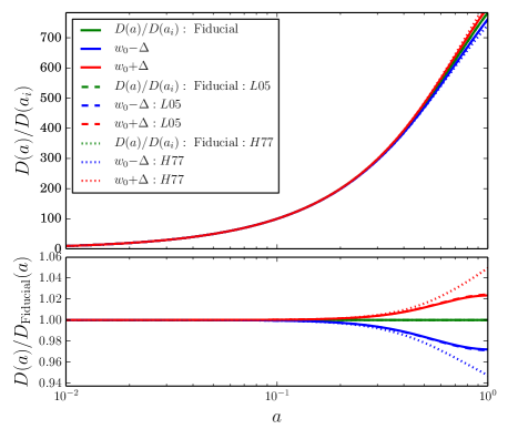
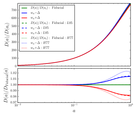
Figure 1 compares the time evolution of the linear growth factor for the four dark energy models listed in Table 2 with that of our fiducial model. The left panel shows the results for the two constant $w_{0}$ models and the right panel the same but for the $w_{a}\neq 0$ models. All of the growth functions have been normalised to have the same amplitude at the initial time $a_{i}$. The solid line denotes the results from the 4th order Runge-Kutta method. We see that a 10% variation in $w_{0}$ will lead to growth variations of $\pm 2.5\%$ and that variations in $w_{a}=\pm 0.2$ lead to variations of the order $\pm 1.5\%$, and roughly double that for their impact on the power spectrum.

The figure also shows the growth functions that you would get if you were to assume that the solution of Heath (1977) would hold for the case of pressured fluids (for more details and discussion see Appendix A). As the figure clearly shows, the growth functions from the Heath approach are inaccurate at the level of several percent for the dark energy models of interest and so should not be used for model building and predictions where high accuracy is required.

Lastly, the figure also shows the result of evaluating the approximate expression (dashed lines in Fig. 1):

$$D(a)=ag(a)=a\exp\left[\int_{a_{i}}^{a}\frac{da}{a}\left(\Omega_{\rm m}^{\gamma}(a)-1\right)\right]\ ,$$ (18)

where $\gamma=0.55+0.05\left[1-w(a=0.5)\right]$ (Linder, 2005). This provides an excellent description (of the order $\sim$0.1% precision) of the variations in the growth for the dark energy models considered. However, since this also involves a numerical integral we recommend the reader to code up the Runge-Kutta solution, since it is more general and flexible.

4 The measured power spectra

4.1 Estimating the power spectrum

For a given realisation of the density field, an estimator for the power in a given Fourier mode is:

$$\hat{P}({\bf k}_{1},{\bf k}_{2})={V_{\mu}}\delta({\bf k}_{1})\delta({\bf k}_{2})\delta^{K}_{{\bf k}_{1}+{\bf k}_{2}=\bf 0}\ ,$$ (19)

where $V_{\mu}=L^{3}$ is the volume of the simulation. However, the noise in such an estimate is very large and in order to overcome this one must sum over a set of Fourier wavemodes in a thin $k$-shell. Introducing the binning function $\tilde{\Pi}_{k}({\bf q})=1$ for $|{\bf q}|\in[k-\Delta k/2,k+\Delta k/2]$ and zero otherwise, the power spectrum estimate averaged over a bin of width, $\Delta k$, is given by

$$\hat{P}(k)=\int d^{3}{\bf q}_{1}\int d^{3}{\bf q}_{2}\,\delta^{D}\!({\bf q}_{1}+{\bf q}_{2})\frac{\hat{P}({\bf q}_{1},{\bf q}_{2})\tilde{\Pi}_{k}({\bf q}_{1})\tilde{\Pi}_{k}({\bf q}_{2})}{V_{P}(k)}\$$

$$\ =\int d^{3}{\bf q}_{1}\frac{\hat{P}({\bf q}_{1},-{\bf q}_{1})\tilde{\Pi}_{k}({\bf q}_{1})\tilde{\Pi}_{k}(-{\bf q}_{1})}{V_{P}(k)}$$

$$\ =\frac{{V_{\mu}}}{V_{P}(k)}\int d^{3}{\bf q}_{1}\left|\delta({\bf k}_{1})\right|^{2}\tilde{\Pi}_{k}(q_{1})\ ,$$ (20)

where

$$V_{P}(k) \equiv \!\!\int d^{3}{\bf q}_{1}\int d^{3}{\bf q}_{2}\delta_{D}({\bf q}_{1}+{\bf q}_{2})\tilde{\Pi}_{k}({\bf q}_{1})\tilde{\Pi}_{k}({\bf q}_{2})$$ (21)

$$= \!\!\int d^{3}{\bf q}_{1}\tilde{\Pi}_{k}({\bf q}_{1})\tilde{\Pi}_{k}(-{\bf q}_{1})$$

$$= \!\!\int d^{3}{\bf q}_{1}\tilde{\Pi}_{k}({\bf q}_{1})=4\pi k^{2}\Delta k\left[1+\frac{1}{12}\left(\frac{\Delta k}{k}\right)^{2}\right]\$$

is the volume of a spherical shell satisfying these conditions. A practical implementation of the above estimator for $N$-body simulations is described in Smith et al. (2003) and Jing (2005).

The computation of the power spectrum that we employ is embedded in the Gadget-3 code itself and so makes efficient use of the built-in domain decomposition routines and also the fast MPI parallel FFTs as implemented by FFTW (Johnson & Frigo, 2008). In brief, the simulation particles are distributed on to a cubical lattice. The particles are then assigned to the FFT mesh using the ‘cloud-in-cell’ (CIC) mass assignment scheme (note that we reuse the PM force grid for this so the grid size is specified by PMGRID). This gives $\delta_{W}^{\rm d}({\bf x})$ the discrete density field convolved with the CIC window. This we Fourier transform using the FFT algorithm to obtain $\delta_{W}^{\rm d}({\bf k})$. The CIC scheme is then deconvolved using (Jing, 2005):

$$\delta^{\rm d}({\bf k})=\frac{\delta_{W}^{\rm d}({\bf k})}{W_{\rm CIC}({\bf k})}$$ (22)

where

$$W_{\rm CIC}({\bf k})=\prod_{i\in\{x,y,z\}}\left\{\rm Sinc\left(\frac{\pi k_{i}}{2k_{\rm Ny}}\right)\right\}^{2}\ ,$$ (23)

where ${\rm Sinc}(x)\equiv\sin x/x$. The power spectrum of the point-sampled field is then estimated using Eq. (20):

$$\hat{P}^{\rm d}(k)=\frac{{V_{\mu}}}{N_{k}}\sum_{i=1}^{N_{k}}\left|\delta^{\rm d}({\bf k}_{i})\right|^{2}\ ,$$ (24)

where $N_{k}=V_{P}(k)/(2\pi)^{3}/L^{3}$ is the number of Fourier modes in a $k$-space shell.

Following Peebles (1980) the above estimate of the true power spectrum is biased by the addition of the variance from the point sampling procedure. However, this can be corrected for using:

$$P^{d}(k)=P^{c}(k)+\frac{1}{\bar{n}}\ ,$$ (25)

where $P^{c}$ is the power spectrum of the underlying continuous field.

In what follows, we use FFT grids with $N_{\rm grid}=2048$ cells per dimension, and this sets the minimum and maximum spatial frequencies for a given power spectrum to: $k_{\rm min}=2\pi/L$ and $k_{\rm Ny}=\pi N_{\rm grid}/L$. In practice, the power on length scales $k>k_{\rm Ny}$ will get ‘aliased’ to larger spatial scales (Jing, 2005), and so we take the rule of thumb $k_{\rm max}=k_{\rm Ny}/2$. Thus for the $L=500\,h^{-1}{\rm Mpc}$ runs the low-$k$ and high-$k$ cut-offs for the power spectra are $k^{500}_{\rm fun}=0.012\,h\,{\rm Mpc}^{-1}$ and $k^{500}_{\rm max}=6.4\,h\,{\rm Mpc}^{-1}$, respectively. For the $L=3000\,h^{-1}{\rm Mpc}$ box run the cut-offs are: $k^{3000}_{\rm fun}=0.0021\,h\,{\rm Mpc}^{-1}$ and $k^{3000}_{\rm max}=1.072\,h\,{\rm Mpc}^{-1}$.

     

     

     

     

Figure 2: Ratio of the power spectra of the 2LPT initial conditions for the variational runs with the corresponding power spectrum from the fiducial run. All spectra were measured at $z=30$. The points show the measurements from the simulations and the lines show the linear theory from CAMB. The red and blue points denote the positive and negative variation in the particular parameter from the fiducial, which is shown in green. From left to right, the top row shows the variations in $\{w_{0},\,w_{a},\,\Omega_{\rm DE}\}$, the middle row, $\{w_{c}=\Omega_{\rm c}h^{2},\,w_{b}=\Omega_{\rm b}h^{2},\,n_{s}\}$, the bottom row $\{A_{s},\,\alpha_{s}\}$.

4.2 Validation of the initial conditions

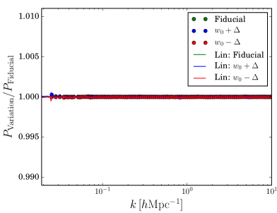
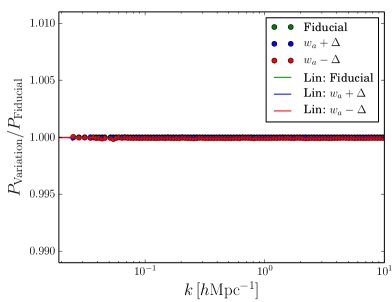
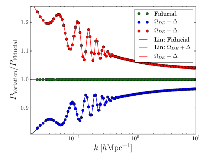
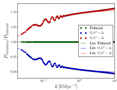
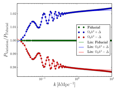
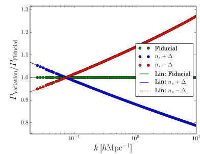
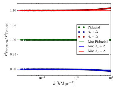
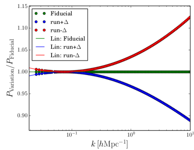
In Figure 2 we present the ratios of the initial power spectra for the variational runs with respect to the fiducial model as generated by our 2LPT code and evolved using Gadget-3 to $z=30$. Each of the eight panels shows the results for variations in one of the cosmological parameters, with all of the others frozen. The positive/negative variation in each of the cosmological parameters is denoted by the red/blue points. The solid red and blue lines denote the predictions from linear theory as obtained from the CAMB code. One can see that taking the ratio with matched phase initial condition means that the cosmic variance has been cancelled on large-scales. We also note that the measured data points and linear predictions agree to very high accuracy, validating the initial density spectra for each simulation.

   

   

Figure 3: Evolution of the nonlinear matter power spectra for the Fiducial Planck-like model as a function of spatial wavenumber. The top left, top-right, bottom left, bottom right sub-figures show the spectra for $z=0$, $z=0.5$, $z=1.0$, and $z=2.0$, respectively. In all panels, the red points with error bars show the mean power spectrum and its 1$\sigma$ errors for the small-box runs ($L=500\,h^{-1}{\rm Mpc}$). The blue points show the results for the large-box run ($L=3000\,h^{-1}{\rm Mpc}$). The shaded blue region gives the predictions for the Gaussian error on the blue points. The dash line shows the linear theory prediction according to CAMB.

   

   

Figure 4: Same as Figure. 4 only showing the composite spectrum generated from the combination of the big-box and small-box runs.

4.3 Evolution of the raw fiducial power spectra

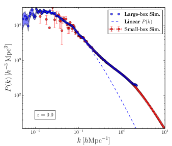
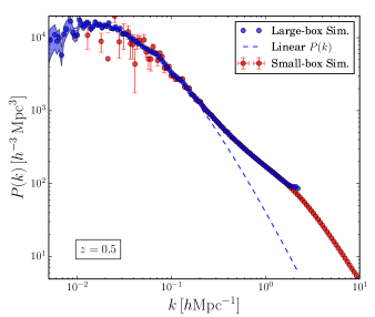
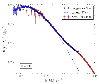
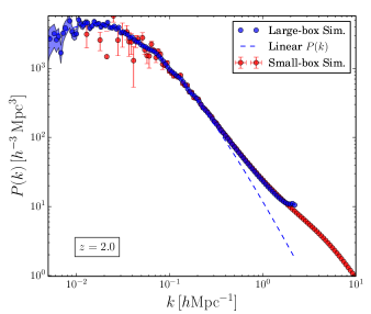
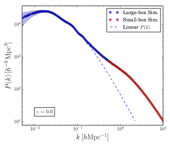
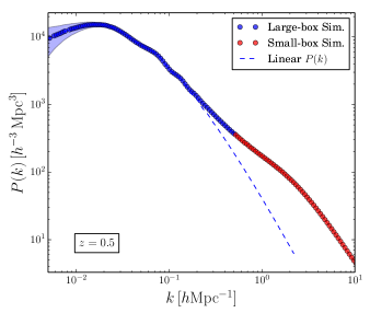
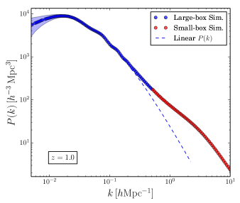
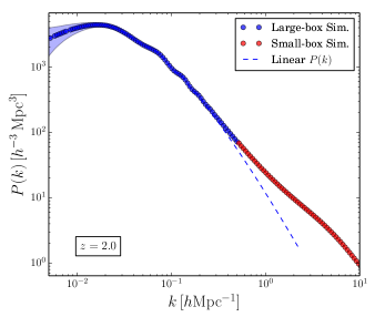
In Figure 4 we show the evolution of the raw matter power spectra measured over several redshifts. In each panel the red points denote the mean of the small-box runs and the error bars are the standard deviation as determined from the 10 realisations. The blue points denote the results from the large-box run and the shaded blue region shows the predicted 1–$\sigma$ error bar that results from assuming the density field is Gaussianly distributed (see for example Scoccimarro, Zaldarriaga & Hui, 1999; Smith, 2009):

$$\sigma^{2}_{P}(k)=\frac{2}{N_{k}}\left[P(k)+\frac{1}{\bar{n}}\right]^{2}\ ,$$ (26)

where $N_{k}$ is the number of Fourier modes in a given $k$-space shell $N_{k}\approx{V_{\mu}}4\pi k^{2}\Delta k\left[1+\left(\Delta k/k\right)^{2}/12\right]/(2\pi)^{3}$ and where $\Delta k$ is the spacing of the $k$-space shell. The dashed blue lines denote linear theory predictions.

We see that there is very good agreement between the large-box and small-box runs on large and quasi-linear scales. There is an increase in the power associated with the big-box relative to the small-box runs at around $k\sim 2\,h\,{\rm Mpc}^{-1}$. This can be attributed to the effects of aliasing. These effects can be mitigated by only considering scales $k<k_{\rm Ny}/2$, where $k_{\rm Ny}=\pi N_{\rm g}/L$, with $N_{\rm g}$ being the size of the FFT grid.

4.4 Construction of the composite fiducial spectra

Rather than using the raw spectra in what follows we construct a super composite of the large- and small-box fiducial runs. We do this by selecting a partition scale $k_{\rm p}$ and then we select all of the modes from the Big-box run with $k<k_{\rm p}$ and all of the data that have $k>k_{\rm p}$ from the small-box runs. We expect a small discontinuity at the partition scale owing to the fact that the large-box runs are more than a factor of 200 times lower resolution than the small-box runs, which means that on small scales we expect the large-box runs to be slightly lower in amplitude. For all spectra we take $k_{\rm p}=0.6\,\,h\,{\rm Mpc}^{-1}$.

In Figure 4 we show the result of the construction of the composite spectrum. We have colour coded the points with $k<k_{\rm p}$ using blue and those with $k\geq k_{\rm p}$ with red. In this plot we have also removed some of the large-scale cosmic variance by rescaling the spectrum of each realisation in the following way:

$$P^{\rm NoCV}(k_{i},a)\!\! = \!\!W(k_{i}|k^{\prime})\hat{P}^{\rm Sim}(k_{i},a)\left[\frac{P^{\rm Lin}(k_{i},a)}{D^{2}(a)P^{\rm Sim}(k,a_{i})}\right]$$ (27)

$$+\left[1-W(k_{i}|k^{\prime})\right]\hat{P}^{\rm Sim}(k_{i})\ ,$$

where we take $k^{\prime}=0.05\,h\,{\rm Mpc}^{-1}$. Note that the shaded region gives the 1$\sigma$ error region computed before any rescaling takes place. The end result is that the composite spectrum smoothly covers more than three orders of magnitude and cuts off at $k\sim 10\,h\,{\rm Mpc}^{-1}$.

5 Comparison with analytic perturbation theory

5.1 Perturbative methods

As the Universe expands small primordial matter over-densities aggregate through gravitational instability. When averaged over sufficiently large enough scales, and on scales smaller than the horizon, the evolution of these fluctuations can be modelled using the Newtonian fluid equations expressed in expanding coordinates. As the system evolves, nonlinear mode coupling takes place and the presence of large-scale wave-modes modulates the growth of structure on all scales (Peebles, 1980; Bernardeau et al., 2002).

As mentioned earlier, in recent years there has been significant progress in developing methods to improve the range of applicability of nonlinear perturbation theory. Of particular note are the RPT and MPT approaches (Crocce & Scoccimarro, 2006b, a; Bernardeau, Crocce & Scoccimarro, 2008). Subsequent research has focused on various extensions of these schemes. We note that currently much interest surrounds the construction of an Effective Field Theory for large-scale structure (Carrasco, Hertzberg & Senatore, 2012). However, we will not explore this here, since as has been shown in Baldauf, Mercolli & Zaldarriaga (2015), the additional complexity and need for a, possibly scale-dependent, free-parameter means that this technique is not generally applicable ‘right out of the box’. Moreover, even when fully calibrated this approach would offer improvements over MPT only on scales where, in this work, we will look to $N$-body simulations for the correct answer. In what follows, we will therefore focus on implementing and testing the MPT method against our runs.

  

Figure 5: Nonlinear power spectrum on large-scales as a function of wavenumber. Left figure, top panel: the absolute power at $z=0$. The solid blue points present the results from our large-box simulation ($L=3000\,h^{-1}{\rm Mpc}$, $N=2048^{3}$) of our Fiducial model. The light shaded band shows the Gaussian prediction of the 1-$\sigma$ errors on the measured data given by Eq. (26). The thick solid line shows the predictions from MPT theory. The thin blue line shows linear theory and the dashed, dotted and dot-dashed lines show the individual contributions to the MPT predictions from the 1-, 2- and 3-point propagators, respectively. The thick solid yellow/gold line presents the correction to the MPTbreeze recipe described in §5.4. Left figure, bottom panel: The ratio of the measurements and MPT theory with respect to the linear theory predictions. Right figure: the same as left figure, but for $z=1$.

5.2 The power spectrum in the Multi-point Propagator Theory

In this theory the matter power spectrum can be expressed as an infinite sum over nonlinear $n$-point propagators:

$$P_{\rm MPT}(k,z)\!\!\! = \!\!\!\sum_{n\geq 1}n!\int\frac{{\rm d}^{3}{\bf q}_{1}}{(2\pi)^{3}}\ldots\frac{{\rm d}^{3}{\bf q}_{n}}{(2\pi)^{3}}\,\delta^{\rm D}({\bf k}-{\bf q}_{1}\dots-{\bf q}_{n})$$ (28)

$$\times\left[\Gamma^{(n)}({\bf q}_{1},\ldots,{\bf q}_{n};z)\right]^{2}P_{0}(q_{1})\ldots P_{0}(q_{n})\ ,$$

where $P_{0}$ denotes the initial matter power spectrum determined at some initial time. The $\Gamma^{(n)}$ are the ‘multi-point propagators’, which can loosely be understood as the memory that the final field at a given point retains from multiple connections to the initial field. More formally, they can be defined:

$$\frac{1}{n!}\,\left<\frac{\delta^{n}\Psi_{a}({\bf k},z)}{\delta\phi_{b_{1}}({\bf q}_{1},z_{i})\dots\delta\phi_{b_{n}}({\bf q}_{n},z_{i})}\right>$$ (29)

$$\equiv\frac{}{}\delta^{\rm D}({\bf k}-{\bf q}_{1}-\dots-{\bf q}_{n})\ \Gamma^{(n)}_{ab_{1}\dots b_{n}}\left({\bf q}_{1},\dots,{\bf q}_{n},z\right),$$

where $\Psi_{a}({\bf k},z)=\{\delta({\bf k},z),\theta({\bf k},z)\}$ is a doublet which denotes the late time density and velocity divergence fields and where $\phi_{a}({\bf k},z_{i})\equiv\Psi_{a}({\bf k},z_{i})$ denotes the doublet at some initial time and when the initial fields are set to start in the growing mode we have that $\phi_{a}({\bf k},z_{i})=u_{a}\delta_{0}({\bf k})$ with $u_{a}=\{1,1\}$. The operation on the left-hand-side of Eq. (29) means take the $n$th functional derivative of the final state with respect to $n$ initial states. The angle brackets mean compute the expectation of the resultant expression. Lastly the above definition for the $n$-point propagators can be connected to the term $\Gamma^{(n)}$ in Eq. (28) through the expression:

$$\Gamma^{(n)}({\bf q}_{1},\ldots,{\bf q}_{t})=\Gamma^{(n)}_{1c_{1}\ldots c_{t}}({\bf q}_{1},\ldots,{\bf q}_{n})\,u_{c_{1}}\ldots u_{c_{t}},$$ (30)

where repeated indices are summed over.

As can be understood from inspection of Eq. (28) one major advantage of the MPT expansion over the standard perturbation theory scheme is that all of the terms in the expansion are clearly positive. Further, as the order $n$ is increased the contributions to the power spectrum appear to contribute to increasingly small scales. Hence, on large-scales, one can confidently truncate the sequence at a finite number of ‘loops’.

5.3 MPT recipe à la MPTbreeze:

In this work we will desire to use the MPT approach to describe the power spectrum in the weakly nonlinear regime, and in order to do this we follow Crocce, Scoccimarro & Bernardeau (2012) and truncate the propagator expansion after the first three terms in Eq. (28). In the diagrammatic language this corresponds to renormalised versions of tree level, one and two loop corrections, respectively. Explicitly, this is:

$$P_{\rm MPT}(k,z) \approx \left[\Gamma^{(1)}(k;z,z_{i})\right]^{2}P_{0}(k,z_{i})$$ (31)

$$+2\int\frac{d^{3}{\bf q}}{(2\pi)^{3}}\left[\Gamma^{(2)}({\bf k}-{\bf q},{\bf q};z,z_{i})\right]^{2}P_{0}(|{\bf k}-{\bf q}|,z_{i})P_{0}(q,z_{i})$$

$$+6\int\frac{d^{3}{\bf q}_{1}}{(2\pi)^{3}}\int\frac{d^{3}{\bf q}_{2}}{(2\pi)^{3}}\,\left[\Gamma^{(3)}({\bf k}-{\bf q}_{1}-{\bf q}_{2},{\bf q}_{1},{\bf q}_{2};z,z_{i})\right]^{2}$$

$$\times P_{0}(|{\bf k}-{\bf q}_{1}-{\bf q}_{2}|,z_{i})P_{0}(q_{1},z_{i})P_{0}(q_{2},z_{i})\ ,$$

and where the 1-, 2- and 3-point propagators are given by:

$$\Gamma^{(1)}\!\! = \!\!D(z,z_{i})F^{(\rm s)}_{1}({\bf q}_{1})e^{\left[f(|{\bf q}_{1}|)D^{2}(z,z_{i})\right]}\ ;$$ (32)

$$\Gamma^{(2)}\!\! = \!\!D^{2}(z,z_{i})F_{2}^{(\rm s)}({\bf q}_{1},{\bf q}_{2})e^{\left[f(|{\bf q}_{1}+{\bf q}_{2}|)D^{2}(z,z_{i})\right]}\ ;$$ (33)

$$\Gamma^{(3)}\!\! = \!\!D^{3}(z,z_{i})F^{(\rm s)}_{3}({\bf q}_{1},{\bf q}_{2},{\bf q}_{3})e^{\left[f(|{\bf q}_{1}+{\bf q}_{2}+{\bf q}_{3}|)D^{2}(z,z_{i})\right]}$$ (34)

where for brevity we have suppressed the arguments of the $\Gamma^{(n)}$ functions. The symmetrised gravitational mode coupling kernels $F_{n}^{(\rm s)}$ up to third order and the function $f(q)$ are given in Appendix B.

Considering Eq. (31), the first term on the right-hand side is directly proportional to the linear power spectrum and the square of the 1-point propagator, which is a direct indicator of the ‘memory’ of the initial conditions on a particular scale to that same scale at late times. The second term is the ‘one-loop’ correction, this term can be simplified as follows: firstly, a quick inspection of the $F^{(\rm s)}_{2}({\bf q}_{1},{\bf q}_{2})$ kernel indicates that it depends only on the magnitudes of the two vector arguments and the cosine of the angle between them. Hence, on choosing the ${\bf k}$ vector to denote the $z$-axis of a spherical polar coordinate system one can immediately integrate out the azimuthal angle. Secondly, the exponential term depends on the sum of the two vector arguments, and by momentum conservation we have that the sum always results in $k$, hence it may be factored out of the integrals. This leaves us with:

$$P_{\rm MPT}^{(1\ell)}(k,z) = \frac{4\pi D^{4}(z,z_{i})}{(2\pi)^{3}}\exp\left[2f(k)D^{2}(z,z_{i})\right]$$ (35)

$$\times\int_{0}^{\infty}dqq^{2}\int_{-1}^{1}d\mu\left[\tilde{F}_{2}^{(\rm s)}(q,k,\mu)\right]^{2}P_{0}(k\psi(y,\mu))P_{0}(q)\ ,$$

where

$$\tilde{F}_{2}^{(\rm s)}=\frac{5}{7}+\frac{1}{2}\left[\frac{\mu-y}{\psi(y,\mu)}\right]\left[\frac{y}{\psi(y,\mu)}+\frac{\psi(y,\mu)}{y}\right]+\frac{2}{7}\left[\frac{\mu-y}{\psi(y,\mu)}\right]^{2}\ ,$$ (36)

with $\psi(y,\mu)\equiv\left(1+y^{2}-2y\mu\right)^{1/2}$ and $y\equiv q/k$. We are thus left with an integration in 2-D which can be rapidly evaluated with a standard Gaussian quadrature routine and we employ repeated use of the GSL standard library routine gsl_integration_qag.

Consider the third term on the right-hand-side of Eq. (31), this is termed the ‘two-loop’ correction and in order evaluate this we first substitute $\Gamma^{(3)}$ in. Again, we notice that exponential term can be extracted. Next, we follow Crocce, Scoccimarro & Bernardeau (2012) and reduce the dimensionality of the integration by one integral through noting the following: without loss of generality we can fix the ${\bf k}$ to lie along the $z$-axis. Next we can restrict ${\bf q}_{1}$ to lie in the $x-z$ plane. Finally, ${\bf q}_{2}$ must be unrestricted. With these choices, the relevant vectors in spherical polar coordinates as:

$${\bf k} = k\,\,(0,0,1)$$

$${\bf q}_{1} = q_{1}(\sin\theta_{1},0,\cos\theta_{1})$$

$${\bf q}_{2} = q_{2}(\sin\phi_{2}\sin\theta_{2},\cos\phi_{2}\sin\theta_{2},\cos\theta_{2}).$$

On integrating out the redundant azimuthal angle $\phi_{1}$ of the ${\bf q}_{1}$ vector we are left with the following 5-D integral

$$P_{\rm MPT}^{(2\ell)}(k,z) = \frac{12\pi D^{6}(z,z_{i})}{(2\pi)^{6}}\exp\left[2f(k)D^{2}(z,z_{i})\right]$$ (38)

$$\times\int_{0}^{\infty}dq_{1}q_{1}^{2}\int_{0}^{\infty}dq_{2}q_{2}^{2}\int_{-1}^{1}d\mu_{1}\int_{-1}^{1}d\mu_{2}\int_{0}^{2\pi}d\phi_{2}\,$$

$$\times\left[\frac{}{}F_{3}^{(\rm s)}({\bf k}-{\bf q}_{1}-{\bf q}_{2},{\bf q}_{1},{\bf q}_{2};z)\right]^{2}$$

$$\times\frac{}{}P_{0}(|{\bf k}-{\bf q}_{1}-{\bf q}_{2}|)P_{0}(q_{1})P_{0}(q_{2})\ ,$$

were $\mu_{1}=\cos\theta_{1}$ and $\mu_{2}=\cos\theta_{2}$. This integral can be efficiently computed using Monte Carlo integration techniques and we employ the Vegas algorithm supplied by the CUBA-4.2 package (Hahn, 2016). Note that in the numerical implementation of the integrals Eqs (35) and (38) we perform the radial integrals over the restricted domain: $q_{i}\in\left[k_{\rm min},k_{\rm max}\right]$ where the lower bound is fixed at $k_{\rm min}=0.001\,h\,{\rm Mpc}^{-1}$ and the upper limit varies according to $k_{\rm max}={\rm max}\left[20k,2\pi\right]$.

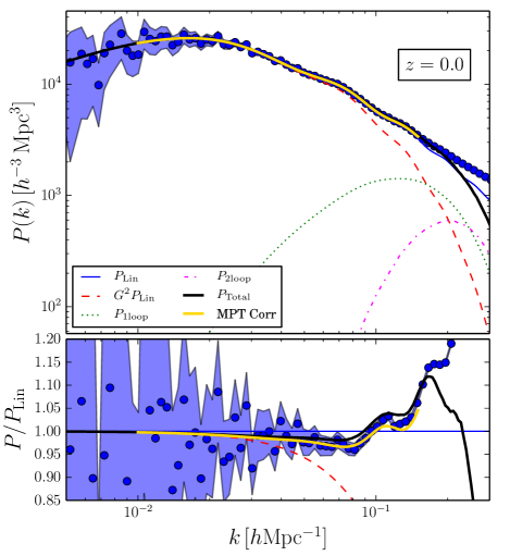
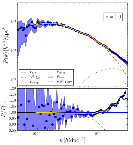
Figure 5 shows the 2-loop calculation of the MPT power spectrum of Eq. (31) evaluated using the above procedure and for our Planck-like fiducial model. The left panel shows $z=0$ and the right $z=1$. The upper panel of each figure shows the absolute power and one can see that the sum of the MPT propagators adds signal to the spectrum at increasingly higher wavemodes. It is interesting to note that at $z=0$, relative to linear theory, there is a 2–3% suppression of power on very large scales ($k\sim 0.07\,h\,{\rm Mpc}^{-1}$), followed by an amplification that starts around $k\sim 0.1\,h\,{\rm Mpc}^{-1}$. In addition, while the 1-point propagator shows tens of percent difference from linear theory at $k\sim 0.1\,h\,{\rm Mpc}^{-1}$, the sum of the 1- and 2-point propagators gives an amplitude that is coincidentally only different by a percent or so.

Figure 5 also compares the theoretical predictions with the composite power spectrum blue points. The shaded blue region shows the 1–$\sigma$ error region, obtained assuming that the density field is a Gaussian random field (c.f. Eq. (26)). The lower panels in the figure show the ratio of the spectra with respect to the linear theory. We see that the MPT calculation describes the results of the simulation up to $k\lesssim 0.15\,h\,{\rm Mpc}^{-1}$ with relatively good accuracy. There are however some small but notable differences, in particular, we see that for the $z=0$ data at $k\gtrsim 0.075\,h\,{\rm Mpc}^{-1}$ the MPT predictions slightly over-predict the data by $\gtrsim 1\%$. For the case of the $z=1$ data this discrepancy is pushed to slightly higher wavenumbers. We therefore explored whether we might correct for this.

5.4 An ad hoc correction to MPT

We found that the MPT predictions and the data could be brought into better agreement by introducing the following ad hoc correction. Considering again the propagator expansion of the power spectrum Eq. (28), we note that if we were to slightly increase the amount of decorrelation of the initial conditions with the final conditions, then this would reduce the predictions on the relevant scales. We find that this can most easily be achieved by recomputing $f(q)$ that appears in Eq. (32) with a nonlinear matter power spectrum model such as halofit2012, which we might call $f_{\rm NL}$ i.e. in Eq. (93) we make the replacement $P_{0}(q)\rightarrow P_{\rm halofit}(q)$ (see Eq. (94)).

Unfortunately, since the resumed 1-point propagator multiplies all of the higher order propagators (see Eqs (33) and (34)), this alteration has the effect of considerably damping all of the loop terms. We obviate this by only using $f_{\rm NL}(q)$ in the computation of the 1-point propagator:

$$\Gamma^{(1)}=D(z,z_{i})F^{(\rm s)}_{1}({\bf q}_{1})e^{\left[f(|{\bf q}_{1}|)D^{2}(z,z_{i})\right]}$$

$$\hskip 2.84544pt\Longrightarrow\Gamma^{(1)}_{\rm NL}=D(z,z_{i})F^{(\rm s)}_{1}({\bf q}_{1})e^{\left[f_{\rm NL}(|{\bf q}_{1}|)D^{2}(z,z_{i})\right]}$$ (39)

and leaving $\Gamma^{(2)}$ and $\Gamma^{(3)}$ unchanged. In implementing this approach we had to pay special attention to the limits of the integral for $f_{\rm NL}(q)$ since we found that the amount of damping was sensitive to the upper limit. After some trial and error we found that adopting the upper limit $k=1.0\,h\,{\rm Mpc}^{-1}$ produced acceptable results. A higher value for this cut-off would lead to too much damping.

In Figure 5 we indicate our correction to the MPT power spectrum implementation by the solid yellow/gold lines. Up to $k=0.1\,h\,{\rm Mpc}^{-1}$ we see that for both of the redshifts considered this recipe leads to improved predictions. We shall therefore adopt this corrected MPT formulation as the means for generating the nonlinear matter power spectrum on scales $k\lesssim 0.1\,h\,{\rm Mpc}^{-1}$. Before continuing, we also point out that our large-box simulation has a volume of $27\,h^{-3}\,{\rm Gpc}^{3}$, and since typical surveys cover a smaller volume we expect that the modelling errors on these large-scales would fall below sample variance errors.

   

   

Figure 6: Evolution of the ratio of the measured nonlinear matter power spectra with the predictions from the halofit2012 model of Takahashi et al. (2012) as a function of spatial wavenumber. The top left, top-right, bottom left, bottom right sub-figures show the spectra for $z=0$, $z=0.5$, $z=1.0$, and $z=2.0$, respectively. In all panels, the red points with error bars show the mean and 1$\sigma$ errors for the power spectra measured from the Planck-2013-like fiducial model simulations in boxes of side $L=500\,h^{-1}{\rm Mpc}$. The solid blue line presents our NGenHalofit model, the dotted line shows the updated halofit2012 model of Takahashi et al. (2012), the dot-dash line shows the original halofit model of Smith et al. (2003), and the dash line shows the linear theory.

6 Comparison with semi-analytic methods

We now compare the power spectra measured from our $N$-body runs with various semi-analytic and emulator methods.

Figure 7: Transition functions as a function of wavenumber. Left panel: variation of transition functions $W$ and $1-W$ with the choice of the cut-scale parameter $k_{\rm cut}$ centred on our fiducial choice. Right panel: same as right panel, but this time showing variation with respect to the width parameter $\sigma_{\rm cut}$. In both panels, the solid lines denote $W$ and the dotted ones give $1-W$.

Figure 8: Transition functions as a function of wavenumber. Left panel: variation of transition functions $W$ and $1-W$ with the choice of the cut-scale parameter $k_{\rm cut}$ centred on our fiducial choice. Right panel: same as right panel, but this time showing variation with respect to the width parameter $\sigma_{\rm cut}$. In both panels, the solid lines denote $W$ and the dotted ones give $1-W$.

6.1 Comparison with halofit and halofit2012

The perturbative methods such as SPT and MPT are unable to describe the evolution of structure once shell-crossing takes place. This we shall refer to as the deeply nonlinear regime. In order to understand how structures collapse and evolve on these scales we need to make use of fully non-perturbative schemes such as $N$-body simulations and study the phenomenology of the structures formed.

The halofit prescription for modelling the nonlinear matter power spectrum, originally developed in Smith et al. (2003) has the following form for the power spectrum:

$$P_{\rm halofit}(k,z|{\bm{\theta}})=P_{\rm L}(k,z|{\bm{\theta}}){\mathcal{G}}(k,z|\bm{\theta})+P_{\rm H}(k,z|\bm{\theta})$$ (40)

where ${\mathcal{G}}(k,z|\bm{\theta})$ represents the quasi-linear suppression and amplification of nonlinear structures that are loosely associated with the phenomenological effects arising from a 2-halo like term and $P_{\rm H}(k,z|\bm{\theta})$ is a 1-halo shot-noise like term (borrowing loosely from the language of the halo model). Parameterised analytic forms for these two functions were devised in Smith et al. (2003) and the best fit parameters were established through fitting to the root mean square difference between the model and a suite of power spectra from $N$-body simulations on small scales and 1-loop SPT on large scales. This approach was recently upgraded in the work of Takahashi et al. (2012) who recalibrated the fitting parameters against a series of improved simulations and extended the method to include a time evolving dark energy equation of state.

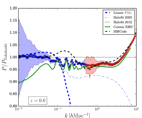
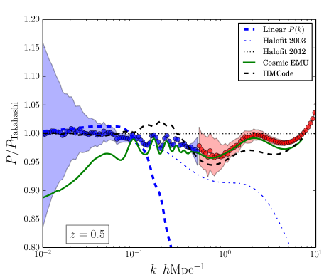
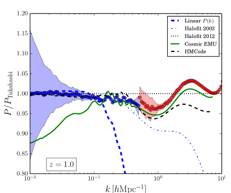
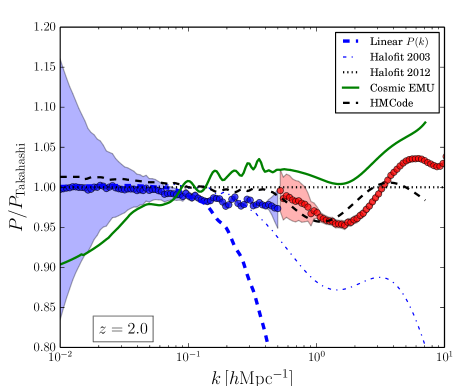
Figure 6 shows the ratio of the composite power spectra derived from our fiducial runs, with the updated halofit model of Takahashi et al. (2012). In all of the panels the blue and red points with error bars denote the composite spectrum from the simulations. The blue dashed line shows the linear theory prediction, which is clearly a poor fit to the measured data for most of the scales of interest. The original halofit algorithm is given by the blue dot-dashed line. This appears to underestimate the true nonlinear power on scales $k>0.2\,h\,{\rm Mpc}^{-1}$ at $z=0$ by roughly 10%. For $k>3\,h\,{\rm Mpc}^{-1}$ this discrepancy rises sharply.

On the other hand, the recalibrated halofit2012 model of Takahashi et al. (2012) provides a good description of the data at the 5% level on all scales. This rises slightly at $k>8\,h\,{\rm Mpc}^{-1}$, however this discrepancy is likely owing to the fact that our data approaches the Nyquist frequency of the FFT mesh at $k\sim 12\,h\,{\rm Mpc}^{-1}$, which leads to a small increase in the power. However, it fails to capture the BAO oscillations on large scales, and also seems to overpredict the amount of structure on quasi-linear scales by $\lesssim 5\%$. This is entirely consistent with the claimed accuracy of the fitting function.

6.2 Comparison with CosmicEMU

We now examine how the predictions from the CosmicEMU model (Heitmann et al., 2014) compare with the estimates from our simulations. We obtained the latest version of the code (Version 3), which included updated constraints from the “Mira-Titan Universe” runs (for details see Lawrence et al., 2017). Since the code returns $P(k)$ in ${\rm Mpc^{3}}$ and $k$ in units of ${\rm Mpc}^{-1}$, we multiply the returned power spectra by $h^{3}$ and the returned wavemodes by $h$ to obtain our standard units. In Figure 6 the results from the CosmicEMU code are presented as the solid green lines. We see that on quasi-linear and nonlinear scales ($k>0.1\,h\,{\rm Mpc}^{-1}$) the emulator does an excellent job to predict the nonlinear power at high precision. At $z=0$ the differences are at the level of a few percent. At $z=0.5$ and $1.0$ the results are in even better agreement. At $z=2$ the results begin to disagree at roughly $\lesssim 5\%$.

On large scales, however, the model appears to be less accurate. For $k<0.1\,h\,{\rm Mpc}^{-1}$ we find that the predictions underestimate the true power by between 5% and 10%. We speculate that this owes to the fact that the CosmicEMU code does not use an externally computed linear theory power spectrum – something that the other methods do by design – but instead interpolates over a set of pre-generated linear spectra (the 37+1 models used to calibrate the fitting function) to make predictions.

6.3 Comparison with HMCode

In Figure 6 we also compare our fiducial runs with the predictions from the HMCode of Mead et al. (2015) (denoted as the black dashed lines in all panels). We use the latest version of CAMB to evaluate this model for our fiducial cosmological model. As can be seen from the figure, this semi-analytic model provides perhaps the best description of our data overall. On large scales it exactly recovers the linear theory. On small scales it is calibrated to the CosmicEMU model, which as we noted above, provides a precise match to our data on these scales. Its main shortcoming appears to be the precise modelling of the quasi-nonlinear regime, in particular the nonlinear processing of the baryon acoustic oscillations in the interval $k\in[0.07\,h\,{\rm Mpc}^{-1},0.5\,h\,{\rm Mpc}^{-1}]$, especially for the $z=0$ data.

Note that we do not consider the PkANN code of Agarwal et al. (2014), since as discussed earlier the quite restrictive set of scales of applicability ($k<1\,h\,{\rm Mpc}^{-1}$) means that this neural network approach, whilst very promising is of limited use for the applications of interest.

Before moving on we also note that in Figure 6 as one goes to higher redshift, a small systematic offset between the spectra from the small- and large-scale box runs emerges. Our investigations of the Millennium Run and Millennium-XXL simulations has shown similar results (see Smith & Simon, 2019). This led us to the conclusion that our simulations suffer from mass-resolution effects (for detailed studies see Heitmann et al., 2010; Schneider et al., 2016). Based on the difference beween the small and large-box runs at the joining scale we therefore estimate that there will be a systematic error in our fiducial spectra of the order $\sim 3\%$. This means that some of the differences that we have noted above may be entirely driven by resolution effects. We also note that we investigated a more elaborate joining scale criterion that was set by finding the $k$-mode at which the size of the sample variance error-bar equalled the error due to Poisson shot-noise. However, this did not yield better results than the empirical joining scale that we adopted through inspection of the power spectral ratios – one obvious problem with this more sophisticated approach was the need to know a priori the nonlinear power spectrum.

7 A new angle on synthesising nonlinear power spectra

Based on the insufficiencies of the previous methods we now describe a new approach to improving the accuracy of the current methods for a wide range of cosmological models, but especially in the vicinity of the peak of the posterior for the Planck data.

7.1 The NGenHalofit method

To start, we assert that on large scales $k<k_{\rm cut}$ the power spectrum can, to high accuracy, be described by a 2-loop MPT calculation and that on smaller scales $k\geq k_{\rm cut}$ it can be well represented by a nonlinear fitting function (we will use the corrected MPT expressions described at the end of §5). Thus our new scheme must enable us to interpolate between these two regimes and we do this using,

$$P_{\rm NGenHalofit}(k,z|\bm{\theta}) = W(k|k_{\rm cut})P_{\rm MPT}(k,z|\bm{\theta})$$ (41)

$$+\left[1-W(k|k_{\rm cut})\right]P_{\rm true}(k,z|\bm{\theta})\ ,$$

where $P_{\rm true}(k)$ is the ‘true’ nonlinear matter power spectrum given the cosmological model and redshift, and is free from noise. For the interpolation function we adopt a scaled error function form,

$$W(k|k_{\rm cut})=\frac{1}{2}\left(1-{\rm Erf}\left[\frac{\log_{10}(k/k_{\rm cut})}{\sqrt{2}\sigma_{\rm cut}}\right]\right)\ ,$$ (42)

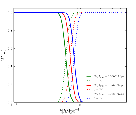
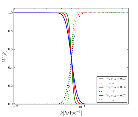
where $k_{\rm cut}$ controls the scale at which the filter $W(k|k_{\rm cut})$ acts as a low-pass filter and $1-W(k|k_{\rm cut})$ acts as a high-pass filter. The strength of the transition is controlled by the parameter $\sigma_{\rm cut}$. Figure 8 shows how the transition functions $W$ and $1-W$ behave for various choices for $k_{\rm cut}$ and $\sigma_{\rm cut}$. After experimenting with various values we found $k_{\rm cut}=0.07\,h\,{\rm Mpc}^{-1}$ and $\sigma_{\rm cut}=0.05$ gave the desired transition scale and speed.

In order to proceed further all we need is the true nonlinear model power spectrum! Unfortunately we do not have access to this, however what we do have access to is discrete realisations of this under the assumption that the simulations provide a proxy for the “truth”. We also have analytic models that are accurate to $<10\%$. Let us denote these as $P_{\rm model}(k)$. One can thus rewrite our desired true spectrum as:

$$P_{\rm true}(k,z|\bm{\theta}) = P_{\rm model}(k,z|\bm{\theta})\frac{P_{\rm true}(k,z|\bm{\theta})}{P_{\rm model}(k,z|\bm{\theta})}$$ (43)

$$= P_{\rm model}(k,z|\bm{\theta})y(k,z|\bm{\theta})\ ,$$

where we have defined a function $y(k,z|\bm{\theta})$ that characterises the deviations from the known analytic model and $|y-1|<0.1$. Let us next perform a Taylor expansion of the deviation function $y(k,z|\bm{\theta})$ with respect to the cosmological parameters $\bm{\theta}$, about some fiducial model $\bm{\theta}_{0}$, whereupon

$$\frac{P_{\rm true}(k,z|\bm{\theta})}{P_{\rm model}(k,z|\bm{\theta})} = y(k,z|\bm{\theta}_{0})+\sum_{i}\left.\frac{\partial y(k,z|\bm{\theta}_{0})}{\partial\theta_{i}}\right|_{\bm{\theta}_{0}}\Delta\theta_{i}$$ (44)

$$+\frac{1}{2}\sum_{ij}\left.\frac{\partial^{2}y(k,z|\bm{\theta}_{0})}{\partial\theta_{i}\partial\theta_{j}}\right|_{\bm{\theta}_{0}}\Delta\theta_{i}\Delta\theta_{j}+\dots\ .$$

If we now factor out the first term from the square brackets on the right-hand-side, then we see that the true power spectrum can be written as:

$$\frac{P_{\rm true}(k,z|\bm{\theta})}{P_{\rm model}(k,z|\bm{\theta})}\!\! = \!\!y(k,z|\bm{\theta}_{0})\left[1+\sum_{i}{\mathcal{R}}_{i}^{(1)}(k,z|{\bm{\theta}_{0}})\Delta\theta_{i}\right.$$ (45)

$$\left.+\frac{1}{2}\sum_{i,j}{\mathcal{R}}_{ij}^{(2)}(k,z|{\bm{\theta}_{0}})\Delta\theta_{i}\Delta\theta_{j}+\dots\right]$$

where we have defined the 1st and 2nd order, power spectral ratio, logarithmic derivative functions as:

$${\mathcal{R}}^{(1)}_{i}(k,z|{\bm{\theta}}) \equiv \frac{\partial\log y(k,z|\bm{\theta})}{\partial\theta_{i}}\ ;$$ (46)

$${\mathcal{R}}^{(2)}_{ij}(k,z|{\bm{\theta}}) \equiv \frac{1}{y(k,z|\bm{\theta})}\frac{\partial^{2}y(k,z|\bm{\theta})}{\partial\theta_{i}\partial\theta_{j}}\ .$$ (47)

Finally, if we back substitute for $y(k,z|\bm{\theta}_{0})$ in the above expression, then on keeping all terms up to quadratic order we arrive at the approximate formula:

$$\frac{P_{\rm true}(k,z|\bm{\theta})}{P_{\rm model}(k,z|\bm{\theta})}\!\! \approx \!\!\frac{P_{\rm true}(k,z|\bm{\theta}_{0})}{P_{\rm model}(k,z|\bm{\theta}_{0})}\left[1+\sum_{i}{\mathcal{R}}_{i}^{(1)}(k,z|{\bm{\theta}}_{0})\Delta\theta_{i}\right.$$ (48)

$$\left.+\frac{1}{2}\sum_{i,j}{\mathcal{R}}_{ij}^{(2)}(k,z|{\bm{\theta}}_{0})\Delta\theta_{i}\Delta\theta_{j}\right]\ .$$

Several points are worth noting: first, if we are exactly evaluating the fiducial model, then $\Delta\theta_{i}=0$ and the bracketed terms vanish, leaving only $y(k,z|\bm{\theta}_{0})$ to recalibrate the $P_{\rm model}$. This can be obtained directly from a set of simulations of the same cosmological model as the fiducial point. Second, the more accurately our assumed model describes the simulated data, the more rapidly our series of derivative functions will converge to zero, i.e. ${\mathcal{R}}^{(1)}\rightarrow 0$ and ${\mathcal{R}}^{(2)}\rightarrow 0$. Third, if $|{\mathcal{R}}^{(1)}|<0.1$ then a 10% calibration would produce power spectrum predictions that are $\lesssim 1\%$ accurate for parameter differences $|\Delta\theta|=\sqrt{\theta_{1}^{2}+\dots+\theta_{N}^{2}}<0.1$. Fourth, in this work we assume that $P_{\rm true}$ can be obtained from $N$-body simulations and on large scales MPT. In the future, it is hoped that if and when new improved analytic models and simulations are available, these ingredients should be easy to interchange, thus providing a rapid upgrade path for this approach.

One can implement this method at several levels. The zeroth order implementation would simply be to drop all of the response functions and so recalibrate our model at the fiducial point. The 1st order implementation would be to include ${\mathcal{R}}^{(1)}$. To do this one needs to generate the vector of first order partial derivatives of the simulated power spectrum with respect to each of the cosmological parameters at the fiducial point. The 2nd order would be to build the Hessian of the power spectrum with respect to the parameters. In this work we will aim to achieve the 1st order correction, but also a hybrid between 1st and 2nd order corrections, since we can populate the diagonal entry of the Hessian using our current data.

7.2 Practical issues

In what follows we shall take $P_{\rm model}\rightarrow P_{\rm Halofit}$ as the approximate model, using the recalibrated model of Takahashi et al. (2012). The recalibration of the approximate model and the nonlinear response functions can be computed from a small set of $N$-body simulations, which we will describe in the following section. However, before we do this there are a few obstacles to overcome in order for the above approach to be practicable.

$\bullet$ Parameter space coverage: One of the above virtues, can also prove to be a drawback to this approach: if one considers large deviations from the fiducial point $\bm{\theta}_{0}$, such that $\Delta\theta_{i}\gtrsim 1$, then the Taylor expansion will break down. Hence, if one desires to perform cosmological parameter estimation using an uninformative prior, then the accuracy of the theoretical model will vary across the parameter space. This gives rise to the pitfall: a blind application of this method may lead to artificially good constraints on the posterior in the regions around the fiducial model where the model is good (see for example the discussion in Marian et al. 2018, in prep. for more details about this effect). We overcome this by making the following modification to the procedure: we replace the second term in the bracket on the right-hand-side of Eq. (48) with:

$$\sum_{i}{\mathcal{R}}_{i}^{(1)}(k,z|{\bm{\theta}_{0}})\Delta\theta_{i}\rightarrow W_{\rm STH}(\bm{\theta})\sum_{i}{\mathcal{R}}_{i}^{(1)}(k,z|{\bm{\theta}_{0}})\Delta\theta_{i}\ ,$$ (49)

where

$$W_{\rm STH}(\bm{\theta}|\bm{\theta}_{\rm cut},\bm{\sigma}^{\theta}_{{\rm cut}})\equiv\prod_{j=1}^{N_{\rm par}}W_{\rm STH}(\Delta\theta_{j}|\theta_{{\rm cut},j},\sigma^{\theta}_{{\rm cut},j})$$ (50)

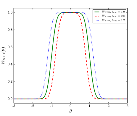
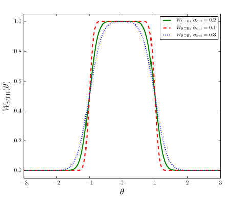
and where $N_{\rm par}$ is the number of cosmological parameters and the function $W_{\rm STH}(\Delta\theta_{j}|\theta_{{\rm cut},j},\sigma^{\theta}_{{\rm cut},j})$ behaves as a smoothed top-hat function centred on the fiducial parameter choice. A similar transition function multiplies the term involving ${\mathcal{R}}_{i}^{(2)}$. In what follows we use the form:

$$W_{\rm STH}(\theta)\!\!\! = \!\!\!-\frac{1}{2}\left\{{\rm Erf}\left[\frac{\theta-\theta_{\rm cut}}{\sqrt{2}\sigma^{\theta}_{\rm cut}}\right]+{\rm Erf}\left[\frac{-\theta-\theta_{\rm cut}}{\sqrt{2}\sigma^{\theta}_{\rm cut}}\right]\right\}\ .$$ (51)

For models with $|\Delta\theta|>\theta_{\rm cut}$, this procedure will guarantee a smooth transition (modulated by $\sigma^{\theta}_{\rm cut}$) to the original theoretical model $P_{\rm model}(k,a|{\bm{\theta}})$, but recalibrated at the fiducial point ${\bm{\theta}_{0}}$. It therefore will enable $P_{\rm model}(k,a|{\bm{\theta}})$ to cover the full parameter space beyond where the Taylor expansion breaks down. Within the vicinity of the fiducial model the theory will become significantly more accurate.

Figure 8 demonstrates how the smoothed top-hat function behaves for an arbitrary parameter for various choices of $\theta_{\rm cut}$ and $\sigma^{\theta}_{\rm cut}$. We discuss how we choose the values of $\theta_{\rm cut}$ in §9.2.

$\bullet$ Smooth functions: As written in Eq. (48), one needs to possess a smooth analytic model for the function $P_{\rm true}(k,z|\bm{\theta}_{0})$ – i.e. the true nonlinear power spectrum at the Fiducial point in our parameter space. Secondly, one also needs the same thing for the response functions ${\mathcal{R}}_{i}^{(1)}(k,z|{\bm{\theta}_{0}})$ – where one function obtains for every cosmological parameter that we consider – and similarly for ${\mathcal{R}}_{i}^{(2)}(k,z|{\bm{\theta}_{0}})$, but this time giving $N(N+1)/2$ functions.

Considering $P_{\rm true}(k,z|\bm{\theta}_{0})$, let us assume that an accurate $N$-body simulation can measure this function over a set of scales $(k_{\rm min}<k<k_{\rm max})$ and over a range of expansion factors $(a_{\rm min}<a<a_{\rm max})$, but that we only have this information at a discrete set of lattice points:

$${\textsf{\bf{P}}_{\rm true}}=\left(\begin{array}[]{ccc}P_{\rm true}(a_{M},k_{1})&\dots&P_{\rm true}(a_{M},k_{N})\\ \vdots&\vdots&\vdots\\ P_{\rm true}(a_{1},k_{1})&\dots&P_{\rm true}(a_{1},k_{N})\end{array}\right)\ ,$$ (52)

where we have suppressed the dependence on the cosmological parameters $\bm{\theta}_{0}$. At this point one might consider using a bicubic interpolation scheme between the lattice points. However, there is a small degree of ambiguity as to how one should do this since the growth between two timesteps is not linear – for instance on large scales we know that $P\propto D^{2}(a)$. One way to obviate such problems is to rescale the elements of the above matrix by the factor $P_{\rm model}(k,z|\bm{\theta}_{0})$:

$${\textsf{\bf{Y}}}=\left(\begin{array}[]{ccc}y(a_{N},k_{1})&\dots&y(a_{M},k_{N})\\ \vdots&\vdots&\vdots\\ y(a_{1},k_{1})&\dots&y(a_{1},k_{N})\end{array}\right)\ .$$ (53)

This ratio has the useful property that for spatial- and time-scales $k\in\{(a_{1},k_{1}),\dots,\,(a_{l},k_{i})\}$ that are large enough and early enough for linear theory to be accurate, $\textsf{\bf{Y}}_{ij}\rightarrow 1$. Nevertheless, provided the model is good, the $y(a_{i},k_{j})\approx 1+\epsilon$, where we will assume $\epsilon\lesssim 0.1$. In the absence of errors in the determination of the $y(a_{i},k_{j})$, one would then simply compute a bi-cubic spline interpolation of the data to obtain the model for $y(a,k)$.

$\bullet$ Noisy data: Our next concern is that the elements of the matrix Y have errors associated with them, since we do not obtain the true $y(a_{i},k_{j})$ directly, but only an estimate $\hat{y}(a_{i},k_{j})$ from an ensemble of simulations. The errors on large scales are dominated by cosmic variance and those on small scales by shot-noise. We may account for this by using ‘Basis splines’ or ‘B-spline’ functions. These differ from interpolating splines in that the resulting curve is not required to pass through each data point. Instead, one constructs a sequence of cubic polynomials that are piece-wise connected together at a set of carefully chosen node points, where the piece-wise polynomials are connected at the node points in such a way that the resultant function is continuous at the nodes. The free parameters that govern each piece-wise polynomial between two nodes are obtained in such a way to reproduce the data in a least squares sense – hence this is also called a smoothing spline (for a detailed discussion of B-splines see de Boor, 1978). In the NGenHalofit code we use the routines provided in the GSL libraries , in particular gsl_bspline_$\star$.

Owing to our desire to accurately capture the baryon acoustic oscillation features, we perform two separate B-spline fits to the data. The first was for the spectra over scales $0.05\,h\,{\rm Mpc}^{-1}<k<0.4\,h\,{\rm Mpc}^{-1}$, with ${\tt NCOEFFS=20}$ and therefore giving ${\tt NBREAK=NCOEFFS-2}=18$ logarithmically spaced spectra node points. This had the desired flexibility to capture rapid features, whilst still being coarse enough to filter out noise. The second B-spline was for the data over scales $0.4\,h\,{\rm Mpc}^{-1}<k<10\,h\,{\rm Mpc}^{-1}$, with ${\tt NCOEFFS=10}$ and therefore giving ${\tt NBREAK=NCOEFFS-2}=8$ logarithmically spaced spectra node points. The B-spline approach required us to specify the variance of the data points and for the small-box fiducial runs we used the errors from the ensemble, whereas for the large-box run we assumed these to follow the Gaussian error model of Eq. (26).

Owing to the fact that we are not aware of a publicly available bicubic B-spline routine, we overcome this problem by making use of the B-spline functions to model each row of the matrix Y. We then recompute the values $y(a_{i},k_{j})\rightarrow y_{\rm B-spline}(a_{i},k_{i})$ and so form the matrix: $\textsf{\bf{Y}}\rightarrow\textsf{\bf{Y}}_{\rm B-spline}$. For this smoothed matrix we are now able to use a bi-cubic spline routine to interpolate between the elements of the $(a_{i},k_{j})$ matrix. We use the bi-cubic spline routine as implemented in the GSL libraries as routines gsl_spline2d_$\star$.

Finally, the approach described above for modelling $y(a,k)$ can be implemented identically for the functions ${\mathcal{R}}_{i}^{(1)}(k,z|{\bm{\theta}_{0}})$ and ${\mathcal{R}}_{i}^{(2)}(k,z|{\bm{\theta}_{0}})$ etc, only one needs to generate arrays of such spline functions.

   

   

Figure 9: Evolution of the ratio of the measured nonlinear matter power spectra with the predictions from the halofit2012 model of Takahashi et al. (2012) as a function of spatial wavenumber. The top left, top-right, bottom left, bottom right sub-figures show the spectra for $z=0$, $z=0.5$, $z=1.0$, and $z=2.0$, respectively. In all panels, the red points with error bars show the mean and 1$\sigma$ errors for the power spectra measured from the Planck-2013-like fiducial model simulations in boxes of side $L=500\,h^{-1}{\rm Mpc}$. The solid blue line presents our NGenHalofit model, the dotted line shows the updated halofit2012 model of Takahashi et al. (2012), the dot-dash line shows the original halofit model of Smith et al. (2003), and the dash line shows the linear theory.

7.3 The new model compared to the fiducial data

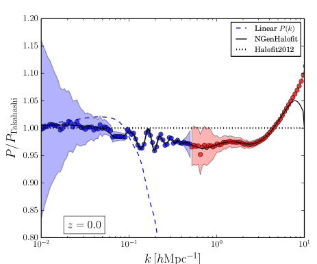
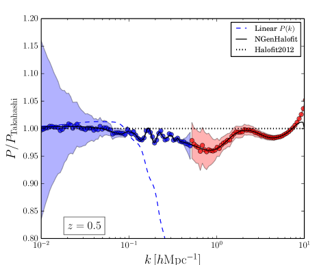
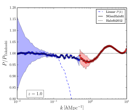
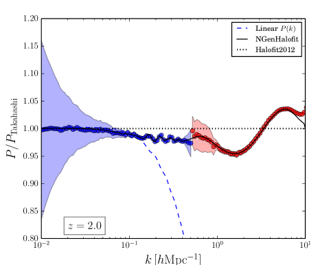
Figure 9 is similar to Fig. 6 and shows the evolution of the ratio of the nonlinear matter power spectrum with respect to the updated halofit2012 model developed by Takahashi et al. (2012). However, in this version of the figure we now compare the measured results with the predictions from our new NGenHalofit code. We see that the data and model predictions are in excellent agreement to high precision on all scales. This good agreement is not surprising, since our zeroth order correction to halofit2012, is to renormalise to match our fiducial simulations through the factor $y(k,z|\bm{\theta}_{0})$.

There are however, two key points to note: first, the solid lines in the figure have been evaluated for an arbitrary set of $k$-modes, meaning that our interpolation scheme is working correctly. Second, one can see that the smoothing spline reproduces most of the features in the data, especially the nonlinear processing of the baryon acoustic oscillations. On the other hand, it has enough restrictions that it is not reproducing all of the noise fluctuations seen in the figure, especially around the joining scale between the spectra from the large- and small-box runs.

8 Cosmology dependence

In this section we examine the cosmological dependence of the nonlinear matter power spectra as a function of scale.

   

   

   

   

Figure 10: Dependence of the power spectrum on variations in the cosmological parameters. All plots show the ratio of the variational models with respect to the fiducial model. Each panel shows the variations for a single parameter as a function of scale. The red and blue points show positive and negative variations, respectively and the point size increases with decreasing redshift, with $z\in\{2,1,0.5,0.0\}$. The dashed lines show the results for linear theory.

8.1 Spectral corrections

For some of our smaller box runs we found that there were some small $\sim 1\%$ deviations from linear theory on very large-scales. In Appendix A we performed an investigation to understand the origin of this error. In turned out to be due to two effects.

First, the code Gadget-3 does not dump snapshots exactly at the listed outputs. There can be small but significant deviations from the requested expansion factor – even for the case of the same cosmological model simulated with different initial conditions. Owing to that, we evolved all of the snapshots to exactly the same set of expansion factors. This was done by assigning a reference list of snapshot expansion factors, and for this we used the fiducial run1 small box set. For each simulation we then computed the linear growth factor to the exact output redshift of the snapshot and also the growth factor to the desired reference expansion factor. The corrected spectrum can then be obtained through linear extrapolation:

$$P^{(1)}_{\rm Sim}(k,a_{*})=\frac{D^{2}(a_{*})}{D^{2}(a_{\rm sim})}P^{(0)}_{\rm Sim}(k,a_{\rm sim})\ ,$$ (54)

where $a_{*}$ and $a_{\rm sim}$ are the desired reference and actual simulated expansion factors, respectively. Note that here we are assuming that the nonlinear spectrum does not evolve appreciably between $a_{\rm sim}$ and $a_{*}$. This is reasonable, since we are considering deviations of the order $\lesssim 1\%$ between $a_{\rm sim}$ and $a_{*}$.

Second, as the Appendix A shows, if one explores how the power spectral modes with $k<0.04\,h\,{\rm Mpc}^{-1}$ evolve compared to linear theory, then in most cases the results are $\lesssim 0.6\%$ agreement. However, for some cases, the differences could be as high as $1.5\%$ (in the appendix we speculate about the cause of this effect). We deal with this by applying a small correction to all of our variation spectra to guarantee that the large-scale modes $k<0.03\,h\,{\rm Mpc}^{-1}$ match linear theory exactly. We estimate the correction through reference to the ratio of the variation to the fiducial model, through:

$$C({\bm{\theta}},a)=\frac{1}{N_{<}}\sum^{N_{<}}_{i}\frac{[P_{\rm Lin}(k_{i},a|{\bm{\theta}})/P_{\rm Lin}(k_{i},a|{\bm{\theta}_{0}})]}{[P^{(1)}_{\rm Sim}(k_{i},a|{\bm{\theta}})/P^{(1)}_{\rm Sim}(k_{i},a|{\bm{\theta}_{0}}]}\ .$$ (55)

where $N_{<}$ are all the modes less than $k=0.03\,h\,{\rm Mpc}^{-1}$. Thus our second correction can be written:

$$P^{(2)}_{\rm Sim}(k,a|{\bm{\theta}})=C({\bm{\theta}},a)P^{(1)}_{\rm Sim}(k,a|{\bm{\theta}})\ ,$$ (56)

Clearly, this correction can only affect the runs with $\bm{\theta}\neq\bm{\theta}_{0}$, since for the fiducial runs $C({\bm{\theta}_{0}},a)\equiv 1$. No such correction is applied to the fiducial runs. On large-scales this is of no consequence, since we make use of the large-box run, for which the large-scale power very accurately reproduces linear theory. However, on small scales, where the small boxes are used, this may lead to a small ($\lesssim 0.5\%$) discontinuity between the large- and small-box solutions at the joining scale (The $z=2$ panel of Fig. 9 shows some evidence of this).

8.2 Power spectral ratios

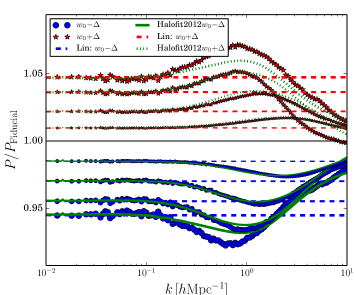
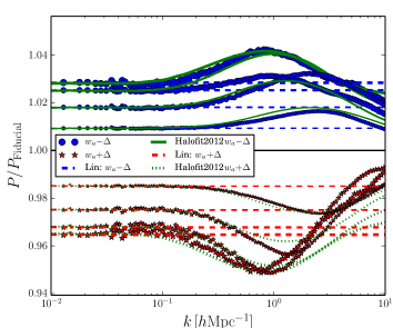
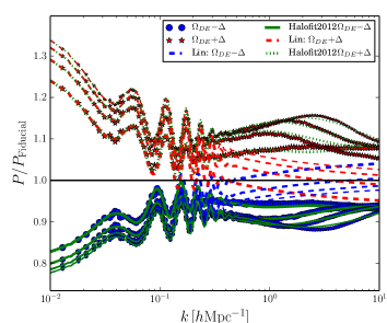
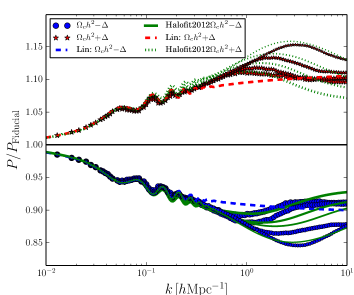
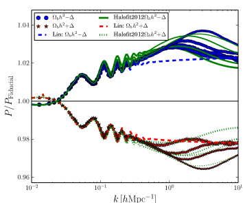
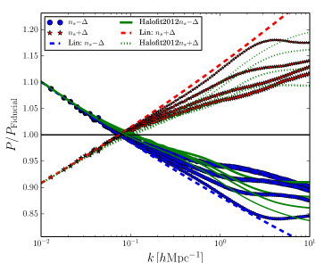
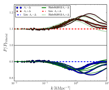
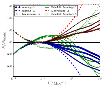
In Figure 10 we show the ratios of the measured nonlinear power spectra for the variations in the cosmological models described in Table 2 with the fiducial power spectrum, as a function of scale and for several epochs. While the absolute value of the power for any given simulation is very noisy on large-scales, owing to the fact that we have used the same phase realisation, the ratio with respect to the corresponding fiducial run cancels out most of the cosmic variance on large-scales, leaving a relatively noiseless quantity. Thus, after implementing the corrections described above, we see that in all of the panels the large-scale ratios accurately match linear theory predictions. Whilst the calibrations were made for scales $k<0.03\,h\,{\rm Mpc}^{-1}$ we clearly see good agreement with the linear theory ratios up to scales of the order $k\sim 0.1\,h\,{\rm Mpc}^{-1}$. On smaller scales, nonlinear evolution drives the measured ratios away from the linear theory prediction.

For the case of the dark energy variations we see that modifications to $w(a)$ primarily affect the linear growth rate on large-scales. However, as we see they also lead to increased/decreased nonlinear power as $w(a)$ becomes more/less negative (see also Linder & Jenkins, 2003). Considering the case of a running power spectral index, we see that for $\alpha$ positive/negative the power is boosted/suppressed on all scales compared to the fiducial model, with the exception of the pivot scale of the primordial power spectrum. For a variation $\alpha=\pm 0.01$ the nonlinear power can be boosted by several percent, with the correction increasing with increasing redshift.

It is interesting to note that the linear theory ratios reach deeper into the nonlinear regime than the absolute value of the linear theory – compare with Fig. 9, where 2-3% departures on scales of $k\sim 0.05\,h\,{\rm Mpc}^{-1}$ are already present for the absolute value.

In the plots we also show how well the halofit2012 mode does at matching the cosmological dependence of the suite of Dämmerung runs (depicted as the thin solid and dashed green lines in the panels). For the parameters $\{w_{0},w_{a},\Omega_{\rm m},\Omega_{\rm c}h^{2},A_{s}\}$ the model does excellently, with deviations being less than a few percent. However, for the parameters $\{\Omega_{\rm b}h^{2},n_{s},\alpha\}$, the prescription does less well with errors being of 5% or more, with the case of the running of the primordial power spectrum being especially bad.

   

   

   

   

Figure 11: Logarithmic derivative of the nonlinear matter power spectrum with respect 8 cosmological parameters considered in this paper as a function of scale. The blue points show the results from the Dämmerung simulations. The dashed lines show the results for linear theory and the solid green lines show the prediction from the updated version of halofit2012 from Takahashi et al. (2012). The point size and line thickness increases with decreasing redshift, with $z\in\{2,1,0.5,0.0\}$.

   

   

   

   

Figure 12: Similar to Fig. 11, except this time the matter power spectra have been rescaled by the predictions from the halofit2012 model before computing the derivative with respect to the cosmological parameters. The magenta solid lines denote the result of applying a smoothing spline function to the measured scaled derivatives. Once again, increasing line thickness and point size corresponds to decreasing redshift with $z\in\{2,1,0.5,0.0\}$.

   

   

   

   

Figure 13: Same as Fig. 12, except here we show the 2nd order derivatives of the power spectra scaled by the halofit2012 predictions with respect to the cosmological parameters.

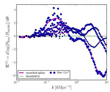
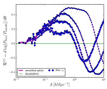
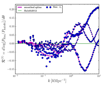
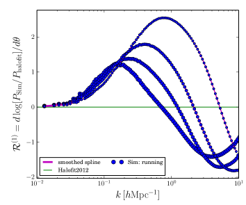
8.3 Derivatives with respect to cosmology

We next turn our attention to the derivatives of the power spectra with respect to the parameter variations. We construct the nonlinear derivatives at the fiducial point $\bm{\theta}_{0}$ in parameter space using the double sided derivative technique from Smith et al. (2014), and for a given cosmological parameter variation this means (suppressing the $k$ and $a$ dependence):

$$\widehat{\frac{\partial P(\bm{\theta})}{\partial\theta_{i}}}\approx\frac{\widehat{P}(\theta_{0,i}+\Delta\theta_{i})-\widehat{P}(\theta_{0,i}-\Delta\theta_{i})}{2\Delta\theta_{i}}+{\mathcal{O}}(\Delta\theta_{i}^{2})\ ,$$ (57)

where the estimate of the logarithmic derivative is given by:

$$\widehat{\frac{\partial\log P(\bm{\theta})}{\partial\theta_{i}}}=\frac{1}{\widehat{P}(\bm{\theta}_{0})}\widehat{\frac{\partial P(\bm{\theta})}{\partial\theta_{i}}}$$ (58)

Note that for the same set of simulations we can also construct the second order derivative:

$$\widehat{\frac{\partial^{2}P({\bm{\theta}})}{\partial\theta_{i}^{2}}} \approx \frac{\widehat{P}(\theta_{0,i}+\Delta\theta_{i})+\widehat{P}(\theta_{0,i}-\Delta\theta_{i})-2\widehat{P}(\theta_{0,i})}{(\Delta\theta_{i})^{2}}$$ (59)

$$+{\mathcal{O}}(\Delta\theta_{i}^{2})\ ,$$

Unfortunately, we do not have enough simulations to fully populate the Hessian matrix $\partial^{2}P(\theta_{i})/\partial\theta_{i}\partial\theta_{j}$ (see §10 for how one can obtain this).

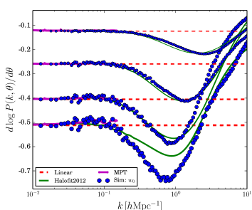
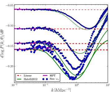
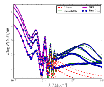
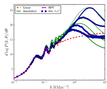
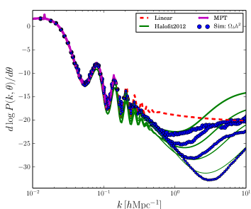
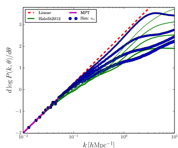
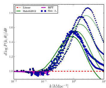
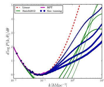
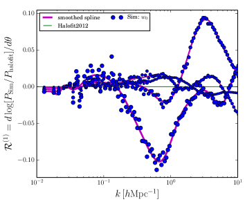
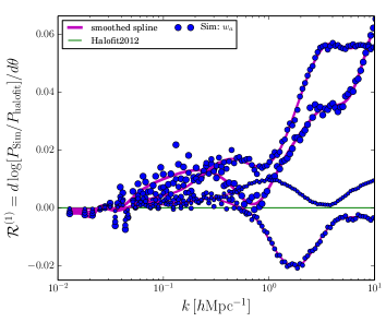
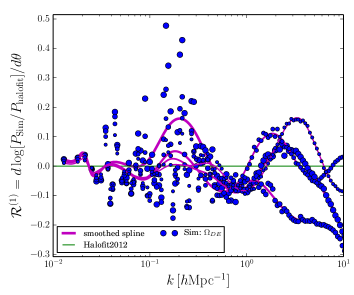
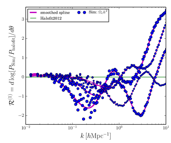
Figure 11 shows the logarithmic derivatives for the 8 cosmological parameter variations listed in Table 2. The blue points denote the measurements at a set of redshifts, with the point size decreasing with increasing redshift. In the each panel we also show the predictions from the linear theory as the red dashed lines and also the predictions from halofit2012 as the green solid lines. We see that on large scales the measured logarithmic derivatives exactly agree with both the linear and nonlinear predictions. This is not too surprising, owing to corrections we have implemented (see §8.1). However, as pointed out in the previous section, while our corrections were made using modes with $k<0.3\,h\,{\rm Mpc}^{-1}$, we see that the agreement between linear theory and the measurements remains very good all the way up to $k\sim 0.1\,h\,{\rm Mpc}^{-1}$. On smaller scales, there are significant deviations.

We also show the predictions for the 2-loop MPT theory calculation evaluated up to $k=0.15\,h\,{\rm Mpc}^{-1}$ as the solid magenta line. We see that the MPT model accurately describes the first order derivatives on these scales. Note that we pushed the calculation to $k=0.3\,h\,{\rm Mpc}^{-1}$ and found strong deviations from the measured results, leading us to believe that the 2-loop answer should be used with care for $k>0.15\,h\,{\rm Mpc}^{-1}$. In our current approach we transition between MPT and our corrected model on scales $k\sim 0.07\,h\,{\rm Mpc}^{-1}$. Nevertheless, one can see that the 2-loop calculation is more accurate than using linear theory, in particular for capturing the cosmology dependence of the nonlinear processing of the BAO features.

We also show the predictions for halofit2012 as the green solid lines. Whilst on the whole it provides a much better description of the measured derivatives, there are some noticeable deviations, and in particular for the parameters $\{\Omega_{\rm b}h^{2},n_{s},\alpha\}$, the model is quite poor.

8.4 Modelling the scaled 1st order and 2nd order derivatives

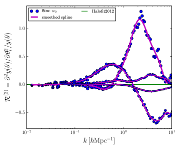
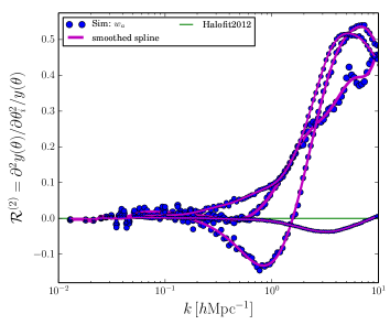
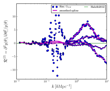
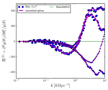
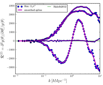
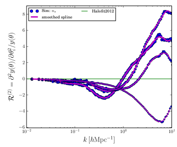
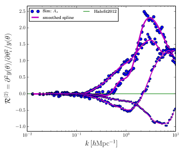
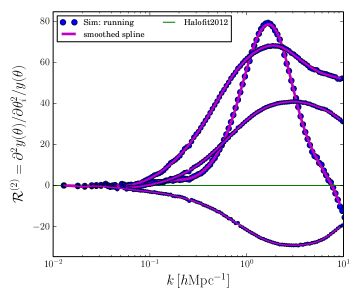
In Figures 12 and 13 we show the first and second order derivative of the power spectra scaled by the predictions from halofit2012 with respect to the cosmological parameters, respectively. If halofit2012 provided a perfect description of the nonlinear evolution, then all of the scaled derivatives would be zero. We see that on large scales ($k\lesssim 0.02\,h\,{\rm Mpc}^{-1}$), indeed the measured derivatives all converge to this value or scatter about it. For the cases of the parameters $\{w_{0},w_{a},\Omega_{\rm DE},n_{s},A_{s}\}$ and for $k<10.0\,h\,{\rm Mpc}^{-1}$ we have ${\mathcal{R}}^{(1)}_{i}=d\log y/d\theta_{i}<0.2$. This suggests that halofit2012 provides a very good description of the cosmology dependence of the nonlinear power spectrum with respect to these parameters.

On the other hand, for the parameters $\{\Omega_{\rm c}h^{2},\Omega_{\rm b}h^{2},\alpha\}$ we see that the scaled derivatives have values $\lesssim 4$ for the scales that we probe. One can also see in Fig. 13 that the scaled 2nd order derivatives for these parameters also have large values. This implies that halofit2012 does not describe the cosmological dependence of the nonlinear power spectrum for these parameters very well. However, we note that, for example, a 10% variation in $\Omega_{\rm c}h^{2}$ away from the fiducial value would imply at most a $\lesssim$40% error in the halofit prediction. Thus if we can calibrate the derivatives then we should produce a method that is significantly more accurate.

Following the approach described in §7.2 we have modelled the measured scaled derivatives using the B-spline approach. The results of this for each parameter are presented in Figures 12 and 13 as the solid magenta lines. Clearly, this smoothed spline function approach captures the trends seen in the data. These functions provide us with the smooth ${\mathcal{R}}_{i}^{(1)}(k,z|{\bm{\theta}}_{0})$ and ${\mathcal{R}}_{ii}^{(2)}(k,z|{\bm{\theta}}_{0})$ components for Eq. (48) on quasi-linear and nonlinear scales. We remind the reader that on large scales the nonlinear predictions are exactly those of the MPT theory.

9 Cosmology dependence of the new model

9.1 Comparison with variational runs

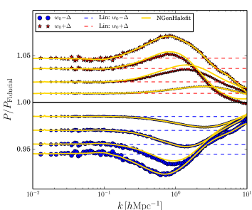
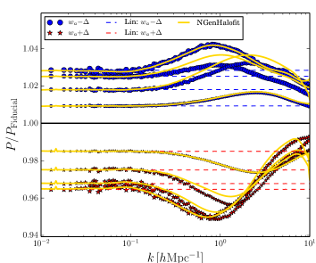
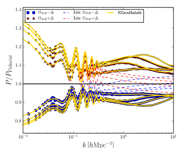
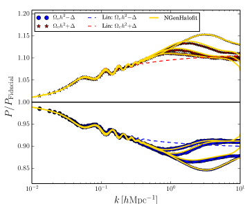
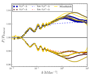
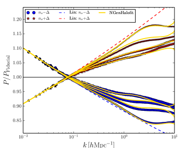
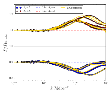
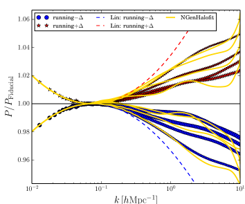
We now turn to the cosmology dependence of NGenHalofit. Figure 14 shows again the ratio of the variational runs with respect to the power spectra from run 1 of the fiducial model. However, this time we show the ability of NGenHalofit to predict the 16 ratios for the 8 parameters – this is shown as the set of solid black lines in each panel.

At first this may not sound like a very stringent test, since we used the variational results to construct the derivatives. However, there is no guarantee that this would enable each of the extreme variations to be accurately predicted, since we are not interpolating. For the case of the parameters $\{w_{0},\Omega_{\rm DE},\Omega_{\rm c}h^{2},n_{s},A_{s}\}$ the fits are virtually perfect. For the remaining parameters one can see that there are some small deviations between the model and the data. This stems from the fact that the linear response appears not to be sufficient to fully capture the variations in these cosmological models and one would need to add in the second order response function to improve this.

Nevertheless, on comparing these results with the predictions from halofit2012, we see that in all cases the predictions from NGenHalofit are better. In particular, for the running of the primordial spectral index, the new approach has significantly improved the predictions and appears to be highly accurate for $k<3\,h\,{\rm Mpc}^{-1}$.

Before moving on, although the ratio of the variation runs with respect to the fiducial model appear to be not too badly described by halofit2012, we point out that the ratio is insensitive to overall calibration errors, since:

$$\frac{P_{\rm true}(k,a|{\bm{\theta}})}{P_{\rm true}(k,a|{\bm{\theta}}_{0})} = 1+\sum_{i}{\mathcal{R}}_{i}^{(1)}(k,z|{\bm{\theta}_{0}})\Delta\theta_{i}$$ (60)

$$+\frac{1}{2}\sum_{i,j}{\mathcal{R}}_{ij}^{(2)}(k,z|{\bm{\theta}_{0}})\Delta\theta_{i}\Delta\theta_{j}+\dots$$

The combination of our exact 2-loop MPT modelling on large scales $(k<0.07\,h\,{\rm Mpc}^{-1})$, our precise modelling of the absolute value of the fiducial power spectra, as demonstrated in Fig. 9, and our again high precision modelling of ${\mathcal{R}}^{(1)}_{i}$ and ${\mathcal{R}}^{(2)}_{ii}$ as demonstrated in Fig. 14 mean that NGenHalofit provides, overall a very accurate description of the power spectra from the Dämmerung run $N$-body data.

   

   

   

   

Figure 14: Dependence of the power spectrum on variations in the cosmological parameters. All plots show the ratio of the variational models with respect to the fiducial model. Each panel shows the variations for a single parameter as a function of scale. The red and blue points show positive and negative variations, respectively and the point size increases with decreasing redshift, with $z\in\{2,1,0.5,0.0\}$. The dashed lines show the results for linear theory.

   

   

   

   

Figure 15: Cosmological parameter step-size below which the Taylor expansion approach is precise to 3%. $\Delta\theta$ is estimated from the simulations using Eq. (63) and we scale it in units of the variation step-sizes used in the Dämmerung runs, and we show this as a function of wavenumber and redshift. The 8 panels show results for each of the cosmological parameter variations simulated. The large red points show results for $z=0$ and the small green points show results for $z=0.5$. In panels 2–7, the blue dashed lines indicate the line $|\Delta\theta|\lesssim 2\left|\Delta\theta_{\rm sim}\right|$, and in panel 1 the line represents $|\Delta\theta|\lesssim 0.5\left|\Delta\theta_{\rm sim}\right|$.

9.2 Estimate of overall precision and accuracy

We now turn to the question of estimating the overall accuracy of the Taylor expansion approach. To do this recall Eq. (48), from this we see that we need both:

$$1>\sum_{i}{\mathcal{R}}_{i}^{(1)}(k,z|{\bm{\theta}}_{0})\Delta\theta_{i}>\frac{1}{2}\sum_{i,j}{\mathcal{R}}_{ij}^{(2)}(k,z|{\bm{\theta}}_{0})\Delta\theta_{i}\Delta\theta_{j}\ .$$ (61)

Let us focus on this relation for a single parameter, with all other parameters held fixed at their fiducial values. Since we are only including the diagonal terms of the Hessian one way to guarantee that the linear order expansion is reasonably accurate would be to require that the second order corrections are a small fraction compared to unity, i.e., for the $i$th parameter, for second order corrections to remain $\lesssim 3\%$ we would require:

$$0.03\lesssim\frac{1}{2}{\mathcal{R}}_{ii}^{(2)}(k,z|{\bm{\theta}}_{0})(\Delta\theta_{i})^{2}$$ (62)

and this would imply that we should take steps in the parameter space away from the fiducial that are given by the inequality:

$$\Longrightarrow\ \ \ \Delta\theta_{i}\lesssim 0.1\sqrt{\frac{6}{{\mathcal{R}}_{ii}^{(2)}(k,z|{\bm{\theta}}_{0})}}\ .$$ (63)

Since we do actually include the second order corrections (at least for variation of a single parameter), this should provide us with a conservative estimate of the precision for a single parameter. On the other hand, since we do not have access to the full matrix ${\mathcal{R}}_{ij}^{(2)}$, it is the case that anything else may be viewed circumspectly. We adopt the value of 3% for the second order correction, since in a recent study by Schneider et al. (2016) the systematic error between various $N$-body codes on small scales was shown to be of this order. Establishing which of the various $N$-body codes is of higher accuracy will be a task for future work.

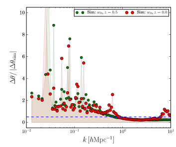
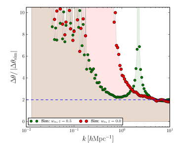
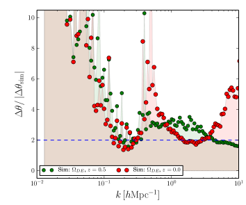
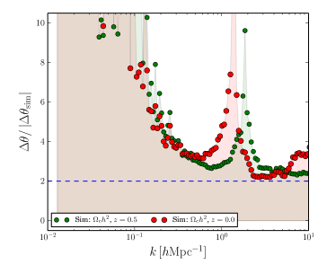
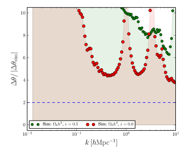
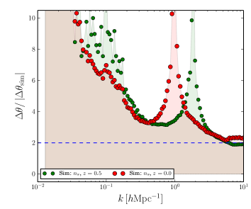
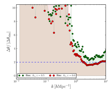
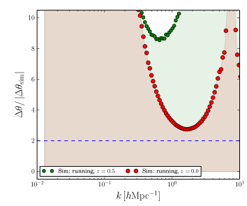
In figure 15 we show the value of $\Delta\theta_{i}$ that obtains from evaluating Eq. (63) and we scale this measured value in units of the parameter step sizes used in the Dämmerung runs. The results are shown as a function of wavenumber and for two redshifts. The plot clearly shows that for all of the parameters considered a step size of $|\Delta\theta|\lesssim 2\left|\Delta\theta_{\rm sim}\right|$ would guarantee that the second order corrections would be below the required value (indicated as the dashed blue line in each panel). The only exception is the case of $w_{0}$, which appears to require the more restricted range of $|\Delta\theta|\lesssim 0.5\left|\Delta\theta_{\rm sim}\right|$.

This leads us to estimate that NGenHalofit should be precise to better than 3% in the cubical region of parameter space given by the range of values: $w_{0}\in\{-1.05,-0.95\}$, $w_{a}\in\{-0.4,0.4\}$, $\Omega_{\rm m,0}\in\{0.21,0.4\}$, $\omega_{\rm c}\in\{0.1,0.13\}$, $\omega_{\rm b}\in\{2.0,2.4\}$, $n_{\rm s}\in\{0.85,1.05\}$, $A_{s}\in\{1.72\times 10^{-9},2.58\times 10^{-9}\}$, $\alpha\in\{-0.2,0.2\}$. When the model under investigation is outside of this region the code predictions smoothly revert back to halofit2012 and so the nominal values for that code apply. Note that we also set the transition speed to be,

$$\sigma^{\theta}_{{\rm cut},i}(k,z)=0.05\left[\theta_{{\rm cut},i}(k,z)-\theta_{0,i}\right]\ .$$ (64)

10 Conclusions & Discussion

In this paper we have generated a suite of 27 high-resolution, $N$-body simulations – the Dämmerung runs. These runs have enabled us to explore the nonlinear evolution of the matter power spectrum in the $w$CDM framework – that is a cosmological model with a time evolving dark energy equation of state. We chose as our fiducial model the best fit parameters from the (Planck Collaboration et al., 2014) data – this we covered with 11 simulations, 10 of which were of comparable resolution to the Millennium Run1 simulation of Springel et al. (2005). The remaining 16 runs modelled the variations in 8 cosmological parameters. We have also performed the first detailed study of the effects of a running primordial power spectral index $\alpha=dn/d\log k$ on the nonlinear matter power spectrum. Our simulations were described in §3 and §4.

In §5 and §6 we compared our measured nonlinear power spectra from the fiducial runs with various analytic and semi-analytic methods. We first explored the ability of MPT theory at the 2-loop level to describe our data. We found that the model reproduced the data to percent accuracy up to $k<0.15\,h\,{\rm Mpc}^{-1}$ at $z=0$. On scales smaller than this, it deviated strongly from the data. We compared our fiducial results with the upgraded halofit model of Takahashi et al. (2012), the EMU code of Heitmann et al. (2014) and the HMCode of Mead et al. (2015). We found that all of these methods described the data on small scales to a precision of 5% – with the EMU code providing the best description on small scales. However, somewhat surprisingly, this code was not able to accurately capture the input large-scale power spectrum, being in error at the level of $\sim 10\%$ on scales of the order $k\sim 0.01\,h\,{\rm Mpc}^{-1}$. Considering all scales, we found that HMCode best described our data overall, but it failed to accurately capture the nonlinear processing of the acoustic oscillations.

In §7 we showed how one could use a suite of simulations to recalibrate a nonlinear power spectrum model to accurately describe the 8-parameter cosmological model that we have examined. The explicit case that we have developed utilises halofit2012 as the underlying base mode, and therefore we dubbed our new improved model NGenHalofit. We also showed that this approach could work to high precision (<1%) for the case of the fiducial model for a range of redshifts and for scales $k<10\,h\,{\rm Mpc}^{-1}$.

In §8 we measured the ratio and logarithmic derivatives of the nonlinear power spectrum with respect to the cosmological parameters. We showed that halofit2012 captured well the dependence on parameters $\{w_{0},w_{a},\Omega_{\rm DE},n_{s},A_{s}\}$. However, in general, it showed variation of the order several percent. For the parameters $\{\Omega_{\rm c}h^{2},\Omega_{\rm b}h^{2},\alpha_{s}\}$ it provided a poor description. We also measured a scaled logarithmic derivative and also the diagonal terms entering the Hessian. This enabled us to build the cosmology dependent corrections for the NGenHalofit model.

We are also interested in constraining variations in the running of the primordial power spectral index $\alpha$ from future large-scale structure measurements, since placing constraints on this may help constrain inflationary models (Vieira, Byrnes & Lewis, 2017). Currently, the only models to do that is the Halofit2012 method. We demonstrated that this model was unable to describe such variations accurately, but that our updated approach enables significantly improved modelling of the impact of spectral running.

Finally, in §8 we used NGenHalofit to predict all of the measured nonlinear spectra ratios. We found that our new approach was able to capture the dependence of the spectrum on cosmology at a level of the order 1% precision.

Future work: The fact that ${\mathcal{R}}^{(1)}_{i}(k,a)\lesssim 4$ for the parameters $\{\Omega_{\rm c}h^{2},\Omega_{\rm b}h^{2},\alpha\}$ suggests that the underlying model halofit2012 did not describe the variations in these parameters as well as the other parameters. One obvious way to improve this implementation would be to include the off-diagonal components of the Hessian matrix. In order to compute these terms one needs to construct the following quantity:

$$\widehat{\frac{\partial^{2}P({\bm{\theta}})}{\partial\theta_{i}\partial\theta_{j}}} \approx \frac{1}{2\Delta\theta_{i}\Delta\theta_{j}}\left[\widehat{P}_{+i,+j}+\widehat{P}_{-i,-j}-2\widehat{P}_{0,0}\right.$$ (65)

$$-\left(\widehat{P}_{+i,0}+\widehat{P}_{-i,0}-2\widehat{P}_{0,0}\right)$$

$$\left.-\left(\widehat{P}_{0,+j}+\widehat{P}_{0,-j}-2\widehat{P}_{0,0}\right)\right]+{\mathcal{O}}(\Delta\theta_{i}\Delta\theta_{j})\ ,$$

where $(i\neq j)$ and where we have introduced the notation:

$$\widehat{P}_{+i,+j} \equiv \widehat{P}(\theta_{0,1},\dots,\theta_{0,i}+\Delta\theta_{i},\dots,\theta_{0,j}+\Delta\theta_{j},\dots,\theta_{0,N})$$

$$\widehat{P}_{+i,-j} \equiv \widehat{P}(\theta_{0,1},\dots,\theta_{0,i}+\Delta\theta_{i},\dots,\theta_{0,j}-\Delta\theta_{j},\dots,\theta_{0,N})$$

$$\widehat{P}_{+i,0} \equiv \widehat{P}(\theta_{0,1},\dots,\theta_{0,i}+\Delta\theta_{i},\dots,\theta_{0,j},\dots,\theta_{0,N})$$

$$\widehat{P}_{0,+j} \equiv \widehat{P}(\theta_{0,1},\dots,\theta_{0,i},\dots,\theta_{0,j}+\Delta\theta_{j},\dots,\theta_{0,N})$$

$$\widehat{P}_{0,0} \equiv \widehat{P}(\theta_{0,1},\dots,\theta_{0,i},\dots,\theta_{0,j},\dots,\theta_{0,N})$$

etc. and where the fiducial point in our $N$-dimensional parameter space is $\bm{\theta}_{0}=\{\theta_{0,1},\dots,\theta_{0,N}\}$. Thus in order to obtain the power spectrum Hessian with respect to the cosmological parameters, we would need to run an additional two simulations for every element of the matrix in the upper half matrix. That is for $N$ cosmological parameters we would need to compute $N(N-1)/2$ elements of the Hessian, each requiring an extra 2 simulations. For the 8 parameters that we are simulating that would mean an extra $8(8-1)/2\times 2=56$ simulations. If we limit this to the terms that depend on the 3 parameters that we have identified then a good approximation would be to add $3(3-1)/2\times 2=6$ runs, and set all other off-diagonal elements to zero. We will explore this in future work.

Another interesting avenue would be to increase parameter space coverage by stitching together Taylor expansion at various points in parameter space. This approach may have advantages over the alternate approach of building emulators using Latin hyper-cube sampling of parameter space, since if the validity of the Taylor expansions encompasses a larger range of parameter space at a given accuracy with fewer simulations than the emulator, then one may need fewer simulations overall to construct solutions over the entirety of the parameter space. We expect that this will be important for future Dark Energy missions like DESI, 4MOST, Euclid, LSST, and WFIRST. We shall leave further discussion of this topic for future work.

Finally, we recognise that in this work we have made no attempt to account for the impact of nonlinear late-time baryonic physics effects on the evolution of matter perturbations. A number of works have established, through theoretical analysis and detailed hydrodynamic simulations, various results (Zhan & Knox, 2004; Jing et al., 2006; Somogyi & Smith, 2010; van Daalen et al., 2011; Schneider et al., 2018). In most cases the inclusion of hot baryons can lead to a supression of the power by $\sim$10%. However, the precise value depends explicitly on the details of the feedback model, resolution of the simulations, the method for simulating the gas physics, and the physics treated. For instance the work of (Jing et al., 2006), besides showing a supression, showed that if radiative heating/cooling effects are turned-off, the matter power spectrum will in fact be enhanced on smaller scales. Similar results were noted in the work of van Daalen et al. (2011) and Semboloni et al. (2011), where gas cooling led to a boost in clustering on small scales. Owing to the fact that this is a very complex problem to disentangle, we shall defer a detailed examination of this area for future works, but note that in the meant time, one may follow the phenomenological approach that was advocated by Semboloni et al. (2011) to build a parameterised baryonic physics template whose physical effects can be marginalised over. We also note that we have neglected to take account the effects of massive neutrinos. We expect that this will also require careful corrections, but note that the work of Bird, Viel & Haehnelt (2012) should still be a viable extension to our model.

Appendix A Linear growth of density modes

A.1 4th order Runge-Kutta solution to linear growth equations

Following §3.3, we now describe how to solve Eq. (14) for the evolution of the linear growth factor. To begin, we introduce a new variable $s=D^{\prime}(a)$. One can now rewrite this second order ODE as a pair of coupled, linear, first order, ordinary differential equations:

$$D^{\prime}(a) = s(a)\ ;$$ (66)

$$s^{\prime}(a) = -\Gamma_{1}(a)s(a)-\Gamma_{2}(a)D(a)\ .$$ (67)

This system is evolved from the initial values $D(a_{i})=a_{i}$ and $s(a_{i})=1$, which owes to the fact that at early times in the evolution we know that $D(a)\propto a$, deep in the matter dominated era. We will solve Eqs (66) and (67) using a 4th order Runge-Kutta method. First let us rewrite the above equations more generally as

$$\frac{dq_{1}}{da} = A(q_{1},q_{2},a)\ ;$$ (68)

$$\frac{dq_{2}}{da} = B(q_{1},q_{2},a)\ ;$$ (69)

where it is the evolution of the variables $q_{1}$ and $q_{2}$ that we wish to solve for and where $A$ and $B$ may be general functions of $q_{1}$, $q_{2}$ and the scale factor $a$. In our case we have $q_{1}(a)=D(a)$ and $q_{2}(a)=s(a)$ and also $A(q_{1},q_{2},a)=q_{2}$ and $B(q_{1},q_{2},a)=-\Gamma_{1}(a)q_{2}-\Gamma_{2}(a)q_{1}$. The 4th order Runge-Kutta solution proceeds from time step $a^{(0)}$ to time step $a^{(1)}=a^{(0)}+\Delta a$ through the following algorithm:

$$k_{1}^{(1)} =A(q_{1}^{(0)},q_{2}^{(0)},a^{(0)})\ ; q_{1}^{(1)} =q_{1}^{(0)}+k_{1}^{(1)}(\Delta a/2)\ ;$$ (70)

$$k_{2}^{(1)} =B(q_{1}^{(0)},q_{2}^{(0)},a^{(0)})\ ; q_{2}^{(1)} =q_{2}^{(0)}+k_{2}^{(1)}(\Delta a/2)\ ;$$ (71)

$$k_{1}^{(2)} =A(q_{1}^{(1)},q_{2}^{(1)},a^{(0)}+\Delta a/2)\ ; q_{1}^{(2)} =q_{1}^{(0)}+k_{1}^{(2)}(\Delta a/2)\ ;$$ (72)

$$k_{2}^{(2)} =B(q_{1}^{(1)},q_{2}^{(1)},a^{(0)}+\Delta a/2)\ ; q_{2}^{(2)} =q_{2}^{(0)}+k_{2}^{(2)}(\Delta a/2)\ ;$$ (73)

$$k_{1}^{(3)} =A(q_{1}^{(2)},q_{2}^{(2)},a^{(0)}+\Delta a/2)\ ; q_{1}^{(3)} =q_{1}^{(0)}+k_{1}^{(3)}\Delta a\ ;$$ (74)

$$k_{2}^{(3)} =B(q_{1}^{(2)},q_{2}^{(2)},a^{(0)}+\Delta a/2)\ ; q_{2}^{(3)} =q_{2}^{(0)}+k_{2}^{(3)}\Delta a\ ;$$ (75)

$$k_{1}^{(4)} =A(q_{1}^{(3)},q_{2}^{(3)},a^{(0)}+\Delta a)\ ; q_{1}^{(4)} =q_{1}^{(0)}+k_{1}^{(4)}\Delta a\ ;$$ (76)

$$k_{2}^{(4)} =B(q_{1}^{(3)},q_{2}^{(3)},a^{(0)}+\Delta a)\ ; q_{2}^{(4)} =q_{2}^{(0)}+k_{2}^{(4)}\Delta a\ ,$$ (77)

where the final estimate of the functions propagated to the next time step is given by:

$$\hat{D}(a^{(0)}+\Delta a) = \hat{D}(a^{(0)})+\left(k_{1}^{(1)}+2k_{1}^{(2)}+2k_{1}^{(3)}+k_{1}^{(4)}\right)\frac{\Delta a}{6}\ ;$$ (78)

$$\hat{s}(a^{(0)}+\Delta a) = \hat{s}(a^{(0)})+\left(k_{2}^{(1)}+2k_{2}^{(2)}+2k_{2}^{(3)}+k_{2}^{(4)}\right)\frac{\Delta a}{6}\ ;$$ (79)

We take $a_{i}=0.001$ and employ 1000 timesteps to reach $a=1.0$. It is useful to note that the above solution for $D(a)$ also provides a solution for the logarithmic growth rate $f(a)\equiv d\log D(a)/d\log a$. Since:

$$\hat{f}(a)\equiv\frac{d\log\hat{D}}{d\log a}=a\frac{\hat{s}(a)}{\hat{D}(a)}\ .$$ (80)

Owing to the fact that the fiducial model is $\Lambda$CDM, we can compare our Runge-Kutta solution with the celebrated integral expression of Heath (1977) for presureless Friedmann-Lemaitre models

$$D_{+}(a)=\frac{5}{2}\Omega_{\rm m,0}H(a)\int_{0}^{a}\frac{da^{\prime}}{\left(a^{\prime}H(a^{\prime})\right)^{3}}\ \ .$$ (81)

Also we can compare this with the well known fitting formula given by Carroll, Press & Turner (1992):

$$D_{\rm CPT}(a)=ag_{\rm CPT}(a,\Omega_{\rm m}(a),\Omega_{\Lambda}(a))\ ,$$ (82)

where

$$g_{\rm CPT}(a,\Omega_{\rm m}(a),\Omega_{\Lambda}(a))\equiv\frac{5}{2}\Omega_{\rm m}(a)\left[\Omega_{\rm m}^{4/7}(a)-\Omega_{\Lambda}(a)+\left(1+\frac{\Omega_{\rm m}(a)}{2}\right)\left(1+\frac{\Omega_{\Lambda}(a)}{70}\right)\right]^{-1}\ .$$ (83)

We can also compare to the approximate growth factor expression from Linder (2005) given in Eq. (18).

The left panel of Figure 16 shows the evolution of $D(a)$ as a function of expansion factor $a$ for our Fiducial cosmological model. It compares the results from our 4th order Runge-Kutta solution (red solid line) with results from a 1st (dot-dashed violet), 2nd order (orange dashed) Runge-Kutta solution, and the Heath (1977) integral solution (green dotted) and the Carroll, Press & Turner (1992) (thin black solid), and the Linder (2005) approximation (thick dashed blue). We find the solutions are accurate to better than 0.1%. The right panel of panel of Figure 16 shows the evolution of the logarithmic growth rate $f(a)$ as a function of expansion factor $a$ for our Fiducial cosmological model. It again compares the results from our 1st, 2nd and 4th order Runge-Kutta solution, and the approximate solution of Linder (2005). The figure shows that the Runge-Kutta solutions are consistent and that the Linder approximation is accurate to better than 0.5%.

   

Figure 16: Left: Upper panel shows the linear growth factor normalised to unity at the present day as a function of the cosmic expansion factor. The red dotted line shows the results for our 4th order Runge-Kutta solution. The solid blue and orange dashed show the 1st and 2nd order Runge-Kutta solutions, respectively. The green dot-dashed lines shows the Heath (1977) integral solution, and the solid black line shows Carroll, Press & Turner (1992). The lower panel shows the ratio of the various results with respect to the 4th order Runge-Kutta solution, expressed as a percentage difference. Right: evolution of the linear growth rate as a function of expansion factor. Again we show the various Runge-Kutta solutions and approximation from Linder (2005). The line styles are as in the left panel.

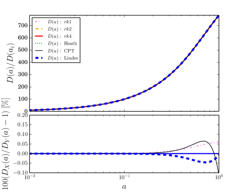
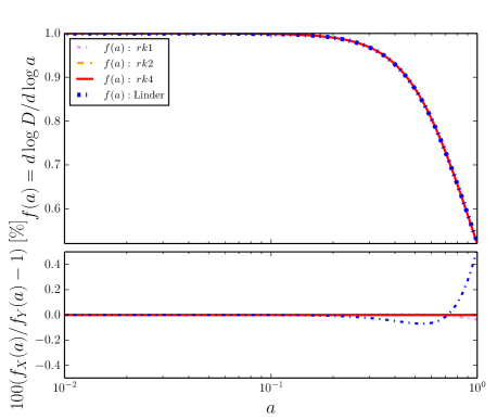
Figure 17 shows the evolution of the logarithmic growth rate as function of expansion factor for the dark energy models considered in this paper. The figure shows that the approximate method of Linder (2005) is an excellent description to our 4th order Runge-Kutta solution, being better than 0.5% for all the times of interest.

   

Figure 17: Logarithmic linear growth rate factor as a function of the cosmic expansion factor $a$. Left and right panels show the results for the four dark energy models listed in Table 2.

   

   

   

Figure 18: Testing the linear growth of the $N$-body simulations. The plot shows how the square of the growth function, normalised in terms of its amplitude at the initial time, divided by the ratio of the power spectrum normalised in terms of its initial value scales as a function of expansion factor. The top-left panel shows the results for the fiducial model: green circles shows results for the $L=500\,h^{-1}{\rm Mpc}$ box and for all scales $k<0.04\,h\,{\rm Mpc}^{-1}$; the blue points are for the $L=3000\,h^{-1}{\rm Mpc}$ run, with the crosses and stars denoting the results for all scales $k<0.04\,h\,{\rm Mpc}^{-1}$ and $k<0.01\,h\,{\rm Mpc}^{-1}$, respectively. The other 8 panels show the same but for the variational runs in the $L=500\,h^{-1}{\rm Mpc}$ boxes and with blue and red points denoting the lower and upper cosmological variation. All of these measurements were based on using all scales $k<0.04\,h\,{\rm Mpc}^{-1}$.

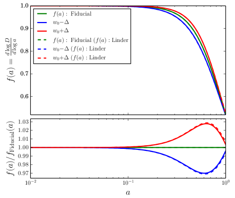
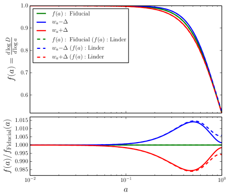
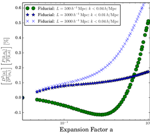
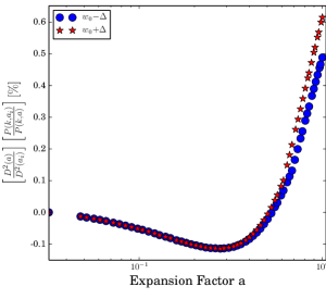
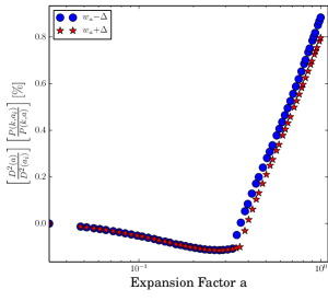
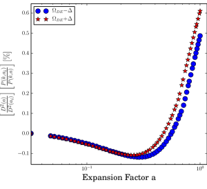
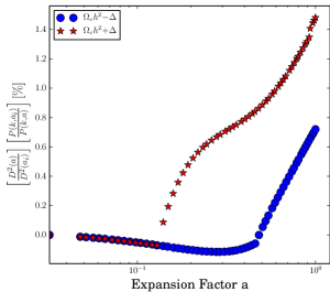
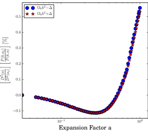
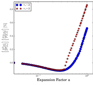
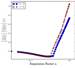
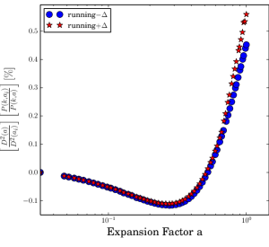
A.2 Linear growth and the Dämmerung simulations

Figure 18 demonstrates how well linear growth is preserved for the largest scale modes in the Dämmerung simulations. The y-axis of the plots shows:

$$r(a)=\frac{1}{N_{<}}\sum_{j\in N<}\frac{D^{2}(a)}{D^{2}(a_{i})}\frac{P(k_{j},a_{i})}{P(k_{j},a)}-1\ .$$ (84)

where $N_{<}$ are all modes with $k<0.04\,h\,{\rm Mpc}^{-1}$. We plot this ratio as a function of the expansion factor $a$ for all of our runs.

First, looking at the small-box fiducial runs (top left panel) we see that the ratio is less than 0.5% for the full range of epochs considered. For the larger box this measure has a higher amplitude. This suggests that there may be some nonlinear mode-coupling at these scales affecting $r$. Changing the cut-off scale from $k=0.04\,h\,{\rm Mpc}^{-1}$ to $k=0.01\,h\,{\rm Mpc}^{-1}$ we see that the linear theory growth is better preserved.

Considering some of the variations we see that same exact trend as for the fiducial run. There are however some outliers where the ratio $r$ deviates to 1.5% – see for example the plot showing the $\Omega_{\rm c}h^{2}+\Delta$ variation. There appears to be something of a discontinuity around $a=0.2$, where we see a sharp upturn in the deviations from linear growth. This seems somewhat nonphysical.

We speculate that this may arise in the following way. Owing to the fact that most super-computer facilities impose a maximum time policy on any one job it is likely that $N$-body runs will need to be restarted and this may happen more than once depending on the strength of clustering. With the code Gadget-3 it is possible to resume a run in one of two ways. The first is from a restartfile, and the second is to restart from a snapshot. In the latter case, position and velocities are synchronised, whereas in the former positions and velocities are different by a half time step, which owes to the structure of the leapfrog time integration. In addition, in the latter case the domain decomposition and tree-construction are done a new, whereas in the former case the exact particle load is preserved as if the simulation was not interrupted. In some cases, the simulations were resumed by starting from snapshot and so potentially this could lead to an error. However, without further investigation, which is beyond the scope of the paper a definitive answer is still to be found. We take these errors into account using the method described in Eq. (55).

Appendix B Auxiliary multi-point propagator theory functions

In order to implement the MPT 2-loop calculation the following results are required.

B.1 Standard perturbation theory kernels

Following Bernardeau et al. (2002, and references therein) the unsymmetrised SPT kernels that we require are:

$$F_{2}({\bf q}_{1},{\bf q}_{2}) = \frac{5}{7}\alpha({\bf q}_{1},{\bf q}_{2})+\frac{2}{7}\beta({\bf q}_{1},{\bf q}_{2})\ ;$$ (85)

$$G_{2}({\bf q}_{1},{\bf q}_{2}) = \frac{3}{7}\alpha({\bf q}_{1},{\bf q}_{2})+\frac{4}{7}\beta({\bf q}_{1},{\bf q}_{2})\ ;$$ (86)

$$F_{3}({\bf q}_{1},{\bf q}_{2},{\bf q}_{3}) = \frac{1}{18}\left[\frac{}{}7\alpha({\bf q}_{1},{\bf q}_{2}+{\bf q}_{3})F_{2}({\bf q}_{2},{\bf q}_{3})+2\beta({\bf q}_{1},{\bf q}_{2}+{\bf q}_{3})G_{2}({\bf q}_{2},{\bf q}_{3})\right.$$ (87)

$$\left.\frac{}{}+7\alpha({\bf q}_{1}+{\bf q}_{2},{\bf q}_{3})G_{2}({\bf q}_{1},{\bf q}_{2})+2\beta({\bf q}_{1}+{\bf q}_{2},{\bf q}_{3})G_{2}({\bf q}_{1},{\bf q}_{2})\right]\ ;$$

where the mode coupling kernels are:

$$\alpha({\bf q}_{1},{\bf q}_{2})\equiv\frac{({\bf q}_{1}+{\bf q}_{2})\cdot{\bf q}_{1}}{q_{1}^{2}}\ \ \ ;\ \ \ \beta({\bf q}_{1},{\bf q}_{2})\equiv\frac{\left[({\bf q}_{1}+{\bf q}_{2})\cdot({\bf q}_{1}+{\bf q}_{2})\right]({\bf q}_{1}\cdot{\bf q}_{2})}{2q_{1}^{2}q_{2}^{2}}\ .$$ (88)

The symmetrised kernels $F_{n}^{(s)}$ are obtained from unsymmetrised kernels by summing over all possible permutations of the arguments and dividing through by the number of permutations:

$$F_{2}^{(\rm s)}({\bf q}_{1},{\bf q}_{2}) = \frac{5}{7}+\frac{1}{2}\frac{{\bf q}_{1}\cdot{\bf q}_{2}}{q_{1}q_{2}}\left(\frac{q_{1}}{q_{2}}+\frac{q_{2}}{q_{1}}\right)+\frac{2}{7}\left[\frac{{\bf q}_{1}\cdot{\bf q}_{2}}{q_{1}q_{2}}\right]^{2}\ ;$$ (89)

$$G_{2}^{(\rm s)}({\bf q}_{1},{\bf q}_{2}) = \frac{3}{7}+\frac{1}{2}\frac{{\bf q}_{1}\cdot{\bf q}_{2}}{q_{1}q_{2}}\left(\frac{q_{1}}{q_{2}}+\frac{q_{2}}{q_{1}}\right)+\frac{4}{7}\left[\frac{{\bf q}_{1}\cdot{\bf q}_{2}}{q_{1}q_{2}}\right]^{2}\ ;$$ (90)

$$F^{(\rm s)}_{3}({\bf q}_{1},{\bf q}_{2},{\bf q}_{3}) = \frac{1}{6}\left[F_{3}({\bf q}_{1},{\bf q}_{2},{\bf q}_{3})+F_{3}({\bf q}_{2},{\bf q}_{1},{\bf q}_{3})+F_{3}({\bf q}_{3},{\bf q}_{1},{\bf q}_{2})\right.$$ (91)

$$\left.+F_{3}({\bf q}_{1},{\bf q}_{3},{\bf q}_{2})+F_{3}({\bf q}_{2},{\bf q}_{3},{\bf q}_{1})+F_{3}({\bf q}_{3},{\bf q}_{2},{\bf q}_{1})\right]\ .$$

The symmetrised version of the $F_{3}$ kernel can be developed further by repeated substitution of Eq. (87) into Eq. (91), to obtain:

$$F^{(\rm s)}_{3}({\bf q}_{1},{\bf q}_{2},{\bf q}_{3}) = \frac{7}{54}\alpha({\bf q}_{1},{\bf q}_{23})F_{2}^{(s)}({\bf q}_{2},{\bf q}_{3})+\frac{1}{27}\left[7\alpha({\bf q}_{23},{\bf q}_{1})+4\beta({\bf q}_{23},{\bf q}_{1})\right]G_{2}^{(\rm s)}({\bf q}_{2},{\bf q}_{3})+2{\rm cyc}\ .$$ (92)

B.2 Auxiliary function for the MPT propagators

In order to compute the MPT propagator damping factors given by Eqs (32)–(34) we need to evaluate the 1D integral:

$$f(k) = \int\frac{d^{3}q}{(2\pi)^{3}}P_{0}(q)\,\frac{1}{504k^{3}q^{5}}\left[6k^{7}q-79k^{5}q^{3}+50q^{5}k^{3}-21kq^{7}+\frac{3}{4}(k^{2}-q^{2})^{3}(2k^{2}+7q^{2})\ln\frac{|k-q|^{2}}{|k+q|^{2}}\,\right]\ .$$ (93)

We do this using the Gaussian quadrature routine gsl_integration_qag provided in the GSL standard library.

Our ad hoc correction to the $f(a)$ function is:

$$f_{\rm NL}(k) = \int_{0}^{q=1\,h\,{\rm Mpc}^{-1}}\!\!\!\frac{dqq^{2}}{2\pi^{2}}\,\frac{P_{\rm halofit2012}(q)}{504k^{3}q^{5}}\left[6k^{7}q-79k^{5}q^{3}+50q^{5}k^{3}-21kq^{7}+\frac{3}{4}(k^{2}-q^{2})^{3}(2k^{2}+7q^{2})\ln\frac{|k-q|^{2}}{|k+q|^{2}}\,\right]\ .$$ (94)

References

- Agarwal et al. (2012) Agarwal S., Abdalla F. B., Feldman H. A., Lahav O., Thomas S. A., 2012, MNRAS, 424, 1409
- Agarwal et al. (2014) Agarwal S., Abdalla F. B., Feldman H. A., Lahav O., Thomas S. A., 2014, MNRAS, 439, 2102
- Alam et al. (2017) Alam S. et al., 2017, MNRAS, 470, 2617
- Angulo et al. (2012) Angulo R. E., Springel V., White S. D. M., Jenkins A., Baugh C. M., Frenk C. S., 2012, MNRAS, 426, 2046
- Baldauf, Mercolli & Zaldarriaga (2015) Baldauf T., Mercolli L., Zaldarriaga M., 2015, PRD, 92, 123007
- Bernardeau et al. (2002) Bernardeau F., Colombi S., Gaztañaga E., Scoccimarro R., 2002, Phys. Rep. , 367, 1
- Bernardeau, Crocce & Scoccimarro (2008) Bernardeau F., Crocce M., Scoccimarro R., 2008, PRD, 78, 103521
- Betoule et al. (2014) Betoule M. et al., 2014, A&A, 568, A22
- Bird, Viel & Haehnelt (2012) Bird S., Viel M., Haehnelt M. G., 2012, MNRAS, 420, 2551
- Carrasco et al. (2014) Carrasco J. J. M., Foreman S., Green D., Senatore L., 2014, Journal of Cosmology and Astro-Particle Physics, 7, 057
- Carrasco, Hertzberg & Senatore (2012) Carrasco J. J. M., Hertzberg M. P., Senatore L., 2012, Journal of High Energy Physics, 9, 82
- Carroll, Press & Turner (1992) Carroll S. M., Press W. H., Turner E. L., 1992, Anual Reviews of Astronomy & Astrophys., 30, 499
- Crocce & Scoccimarro (2006a) Crocce M., Scoccimarro R., 2006a, PRD, 73, 063520
- Crocce & Scoccimarro (2006b) Crocce M., Scoccimarro R., 2006b, PRD, 73, 063519
- Crocce & Scoccimarro (2008) Crocce M., Scoccimarro R., 2008, PRD, 77, 023533
- Crocce, Scoccimarro & Bernardeau (2012) Crocce M., Scoccimarro R., Bernardeau F., 2012, MNRAS, 427, 2537
- Croft et al. (1998) Croft R. A. C., Weinberg D. H., Katz N., Hernquist L., 1998, ApJ, 495, 44
- Davis & Peebles (1983) Davis M., Peebles P. J. E., 1983, ApJ, 267, 465
- de Boor (1978) de Boor C., 1978, A Practical Guide to Splines. Springer-Verlag
- DES Collaboration et al. (2017) DES Collaboration et al., 2017, ArXiv e-prints
- Feldman, Kaiser & Peacock (1994) Feldman H. A., Kaiser N., Peacock J. A., 1994, ApJ, 426, 23
- Goroff et al. (1986) Goroff M. H., Grinstein B., Rey S.-J., Wise M. B., 1986, ApJ, 311, 6
- Hahn (2016) Hahn T., 2016, Comput. Phys. Commun., 207, 341
- Hamilton et al. (1991) Hamilton A. J. S., Kumar P., Lu E., Matthews A., 1991, ApJL, 374, L1
- Heath (1977) Heath D. J., 1977, MNRAS, 179, 351
- Heitmann et al. (2009) Heitmann K., Higdon D., White M., Habib S., Williams B. J., Lawrence E., Wagner C., 2009, ApJ, 705, 156
- Heitmann et al. (2014) Heitmann K., Lawrence E., Kwan J., Habib S., Higdon D., 2014, ApJ, 780, 111
- Heitmann et al. (2010) Heitmann K., White M., Wagner C., Habib S., Higdon D., 2010, ApJ, 715, 104
- Jain & Bertschinger (1994) Jain B., Bertschinger E., 1994, ApJ, 431, 495
- Jing (2005) Jing Y. P., 2005, ApJ, 620, 559
- Jing et al. (2006) Jing Y. P., Zhang P., Lin W. P., Gao L., Springel V., 2006, ApJL, 640, L119
- Johnson & Frigo (2008) Johnson S., Frigo M., 2008, http://www.fftw.org/
- Juszkiewicz (1981) Juszkiewicz R., 1981, MNRAS, 197, 931
- Kaiser (1992) Kaiser N., 1992, ApJ, 388, 272
- Köhlinger et al. (2017) Köhlinger F. et al., 2017, ArXiv e-prints
- Komatsu et al. (2009) Komatsu E. et al., 2009, ApJS, 180, 330
- Lawrence et al. (2017) Lawrence E. et al., 2017, ApJ, 847, 50
- Lawrence et al. (2010) Lawrence E., Heitmann K., White M., Higdon D., Wagner C., Habib S., Williams B., 2010, ApJ, 713, 1322
- Lewis, Challinor & Lasenby (2000) Lewis A., Challinor A., Lasenby A., 2000, Astrophys. J., 538, 473
- Lima & Hu (2004) Lima M., Hu W., 2004, PRD, 70, 043504
- Linder (2005) Linder E. V., 2005, PRD, 72, 043529
- Linder & Jenkins (2003) Linder E. V., Jenkins A., 2003, MNRAS, 346, 573
- Loeb & Zaldarriaga (2004) Loeb A., Zaldarriaga M., 2004, Physical Review Letters, 92, 211301
- Ma & Fry (2000) Ma C., Fry J. N., 2000, ApJ, 543, 503
- Makino, Sasaki & Suto (1992) Makino N., Sasaki M., Suto Y., 1992, PRD, 46, 585
- Mead et al. (2016) Mead A. J., Heymans C., Lombriser L., Peacock J. A., Steele O. I., Winther H. A., 2016, MNRAS, 459, 1468
- Mead et al. (2015) Mead A. J., Peacock J. A., Heymans C., Joudaki S., Heavens A. F., 2015, MNRAS, 454, 1958
- Miralda-Escude (1991) Miralda-Escude J., 1991, ApJ, 380, 1
- Navarro, Frenk & White (1997) Navarro J. F., Frenk C. S., White S. D. M., 1997, ApJ, 490, 493
- Peacock & Dodds (1994) Peacock J. A., Dodds S. J., 1994, MNRAS, 267, 1020
- Peacock & Dodds (1996) Peacock J. A., Dodds S. J., 1996, MNRAS, 280, L19
- Peacock & Smith (2000) Peacock J. A., Smith R. E., 2000, MNRAS, 318, 1144
- Peebles (1980) Peebles P. J. E., 1980, The large-scale structure of the universe. Research supported by the National Science Foundation. Princeton, N.J., Princeton University Press, 1980. 435 p.
- Planck Collaboration et al. (2014) Planck Collaboration et al., 2014, A&A, 571, A16
- Reed et al. (2013) Reed D. S., Smith R. E., Potter D., Schneider A., Stadel J., Moore B., 2013, MNRAS, 431, 1866
- Scherrer & Bertschinger (1991) Scherrer R. J., Bertschinger E., 1991, ApJ, 381, 349
- Schneider et al. (2016) Schneider A. et al., 2016, Journal of Cosmology and Astro-Particle Physics, 4, 047
- Schneider et al. (2018) Schneider A., Teyssier R., Stadel J., Chisari N. E., Le Brun A. M. C., Amara A., Refregier A., 2018, arXiv e-prints
- Scoccimarro et al. (2012) Scoccimarro R., Hui L., Manera M., Chan K. C., 2012, PRD, 85, 083002
- Scoccimarro, Zaldarriaga & Hui (1999) Scoccimarro R., Zaldarriaga M., Hui L., 1999, ApJ, 527, 1
- Seljak (2000) Seljak U., 2000, MNRAS, 318, 203
- Semboloni et al. (2011) Semboloni E., Hoekstra H., Schaye J., van Daalen M. P., McCarthy I. G., 2011, MNRAS, 417, 2020
- Smith (2009) Smith R. E., 2009, MNRAS, 1337
- Smith et al. (2003) Smith R. E. et al., 2003, MNRAS, 341, 1311
- Smith et al. (2014) Smith R. E., Reed D. S., Potter D., Marian L., Crocce M., Moore B., 2014, MNRAS, 440, 249
- Smith, Scoccimarro & Sheth (2007) Smith R. E., Scoccimarro R., Sheth R. K., 2007, PRD, 75, 063512
- Smith & Simon (2019) Smith R. E., Simon P., 2019, ArXiv e-prints
- Somogyi & Smith (2010) Somogyi G., Smith R. E., 2010, PRD, 81, 023524
- Springel (2005) Springel V., 2005, MNRAS, 364, 1105
- Springel et al. (2005) Springel V. et al., 2005, Nature, 435, 629
- Takahashi et al. (2012) Takahashi R., Sato M., Nishimichi T., Taruya A., Oguri M., 2012, ApJ, 761, 152
- van Daalen et al. (2011) van Daalen M. P., Schaye J., Booth C. M., Dalla Vecchia C., 2011, MNRAS, 415, 3649
- Vieira, Byrnes & Lewis (2017) Vieira J. P. P., Byrnes C. T., Lewis A., 2017, ArXiv e-prints
- Vishniac (1983) Vishniac E. T., 1983, MNRAS, 203, 345
- White et al. (1993) White S. D. M., Navarro J. F., Evrard A. E., Frenk C. S., 1993, Nature, 366, 429
- Zhan & Knox (2004) Zhan H., Knox L., 2004, ApJL, 616, L75