Null controllability of parabolic equations with interior degeneracy and one-sided control

Abstract.

For $\alpha\in(0,2)$ we study the null controllability of the parabolic operator

$$Pu=u_{t}-(|x|^{\alpha}u_{x})_{x}\qquad(1<x<1),$$

which degenerates at the interior point $x=0$, for locally distributed controls acting only one side of the origin (that is, on some interval $(a,b)$ with $0<a<b<1$). Our main results guarantees that $P$ is null controllable if and only if it is weakly degenerate, that is, $\alpha\in(0,1)$. So, in order to steer the system to zero, one needs controls to act on both sides of the point of degeneracy in the strongly degenerate case $\alpha\in[1,2)$.

Our approach is based on spectral analysis and the moment method. Indeed, we completely describe the eigenvalues and eigenfunctions of the associated stationary operator in terms of Bessel functions and their zeroes for both weakly and strongly degenerate problems. Hence, we obtain lower $L^{2}$ bounds for the eigenfunctions on the control region in the case $\alpha\in[0,1)$ and deduce the lack of observability in the case of $\alpha\in[1,2)$. We also provide numerical evidence to illustrate our theoretical results.

1. Introduction

1.1. Presentation of the problem and main results

Degenerate parabolic equations have received increasing attention in recent years because of their connections with several applied domains such as climate science ([12, 13], [65], [35], [23]), populations genetics ([26, 27]), vision ([52]), and mathematical finance ([8])—just to mention a few. Indeed, in all these fields, one is naturally led to consider parabolic problems where the diffusion coefficients lose uniform ellipticity. Different situations may occur: degeneracy (of uniform ellipticity) may take place at the boundary or in the interior of the space domain. Moreover, the equation may be degenerate on a small set or even on the whole domain.

From the point of view of control theory, interesting phenomena have been pointed out for degenerate parabolic equations. We refer the reader to [17, 18] and the discussion below for the study of null controllability of boundary-degenerate parabolic operators. A similar analysis for interior-degenerate equations, associated with certain classes of hypoelliptic diffusion operators, was developed in [5, 6] (see also [7]) for Grushin type structures, and in [4] for the Heisenberg operator.

In this paper, intrigued by numerical tests (section 8), we investigate the null controllability of a degenerate parabolic operator in one space dimension, which degenerates at a single point inside the space domain, under the action of a locally distributed control supported only on one side of the domain with respect to the point of degeneracy. In formulas, we consider the problem

(1.1) $$\begin{cases}u_{t}-(|x|^{\alpha}u_{x})_{x}=h(x,t)\chi_{(a,b)}(x),\quad x\in(-1,1)\\ u(-1,t)=0=u(1,t),\\ u(x,0)=u_{0}(x),\end{cases}$$

assuming either $0<a<b<1$ or $-1<a<b<0$. Observe that this is the most general form a locally distributed control can be reduced to for the above operator.

In brief, we will prove that null controllability:

• fails for $\alpha\in[1,2)$,

• holds true when $\alpha\in[0,1)$.

Consequently, the controllability properties of the above operator, when degeneracy occurs inside the domain, are quite different from those of boundary degeneracy described in [17, 18]. In particular, in order for (1.1) to be null controllable when $\alpha\in[1,2)$, the control support must lie on both sides of the degeneracy point. We now proceed to describe our results more precisely and comment on the literature on this subject.

The case of boundary degeneracy was addressed in [16, 17] for equations in one space dimension, that is, for the problem

(1.2) $$\begin{cases}u_{t}-(x^{\alpha}u_{x})_{x}=h(x,t)\chi_{(a,b)}(x),\quad x\in(0,1)\\ \begin{cases}u(0,t)=0=u(1,t)&\text{ if }\alpha\in[0,1),\\ (x^{\alpha}u_{x})(0,t)=0=u(1,t)&\text{ if }\alpha>1,\end{cases}\\ u(x,0)=u_{0}(x).\end{cases}$$

For the above equation, by deriving Carleman estimates with degeneracy-adapted weights, it was proved that null controllability holds if and only if $\alpha\in[0,2)$. These results were later extended in various directions—yet still limited to boundary degeneracy, see [18] and the references therein.

The analysis of problem (1.1) that we develop in the present paper, based on a detailed study of the associated spectral problem, allows us to discover some interesting properties, both positive and negative from the point of view of null controllability. More precisely, we obtain:

• Negative results for $\alpha\in[1,2)$. This fact is a little surprising if compared with the behaviour of the usual problem (1.2). The negative result we prove means that, when $\alpha\in[1,2)$, the degeneracy is too strong to allow the control to act on the other side of the domain with respect to the point of degeneracy. However, null controllability still holds true for those initial condition that are supported in the same region as the control.

• Positive results for $\alpha\in[0,1)$. The proof of the fact that the control is sufficiently strong to cross the degeneracy point does require to use fine properties of Bessel functions. We also give a sharp estimate of the blow-up rate of the null controllability cost as $\alpha\to 1^{-}$.

Degenerate parabolic equations with one (or more) degeneracy point inside the domain have also been studied by the flatness method developed by Martin-Rosier-Rouchon in [53, 54, 55] (see also Moyano [59] for some strongly degenerate equations). More specifically, one can use the null controllability result with boundary control derived in [55] to construct a locally distributed control which steers the initial datum to $0$ for $\alpha\in[0,1)$. On the other hand, neither our analysis of the cost in the weakly degnerate case, nor our negative result for the strongly degenerate case seem to be attainable by the flatness approach.

Parabolic equations with interior degeneracy were also considered by Fragnelli-Mugnai in [32, 33], where positive null controllability results were obtained for a general class of coefficients. Their approach, based on Carleman estimates, gives the controllability result when the control region is on both sides of the space domain with respect to the degeneracy point. Indeed, as our negative result shows, strongly degenerate problems ($\alpha\in[1,2)$) fail to be null controllable otherwise. On the other hand, for weakly degenerate problems, Carleman estimates do not seem to lead to null controllability results with the same generality as we obtain in this paper for problem (1.1) (see Proposition 2.8).

Our method is based on a careful analysis of the spectral problem associated with (1.2). As is known from the work of Kamke [41], the eigenvalues of problem (1.1) are related to the zeros of Bessel functions. Indeed this fact has been recently used in a clever way for a boundary control problem by Gueye [38]. When degeneracy occurs inside, the problem looks like a simplified version of the one studied in Zhang-Zuazua [70] in the case of a 1-D fluid-structure model: we solve the problem on both sides of the degeneracy, and we study the transmission conditions. Once the spectral problem is solved, negative results come quite immediately when $\alpha\in[1,2)$. For the positive part, we combine the moment method with general results obtained in [19] concerning the existence of biorthogonal families under general gap conditions on the square roots of the eigenvalues. Then, we complete the analysis with some $L^{2}$ lower bounds for the eigenfunctions on the control region.

The theoretical results of our foundings are completed with a final numerical work which concludes the paper (see section 8). Starting from the pioneering works of J.-L. Lions (see, e.g., [47]), numerical approximation of controllability problems for parabolic equations has become an established matter. Among the rich literature, we quote here the basic results in [50], devoted to the nondegenerate heat equation with boundary control, along with the more recent studies in [9] and the general framework provided in [43].

Most of the literature is concerned with semi-discretized problems and aims at constructing an approximation of the stabilizing control. We will rather use here a fully discrete approximation, and avoid the problem of convergence of approximate stabilizing controls to a limit solution, which is known to be a very ill-conditioned problem (see [10] for a study of the full discretization, as well as a review of the relevant literature). Therefore, the last section should be understood as a numerical illustration of the theoretical results, while a rigorous study of numerical approximations for this problem will be postponed to future works.

1.2. Plan of the paper

• In section 2, we state our results, distinguishing the weakly degenerate case ($\alpha\in[0,1)$) from the strongly degenerate one ($\alpha\in[1,2)$) (the eigenvalues and the eigenfunctions are not the same according to the case we are considering).

• In section 3, we prove the well-posedness of the problem in both cases.

• In section 4, we solve the spectral problem in the strongly degenerate case ($\alpha\in[1,2)$).

• In section 5, we prove our negative and positive null controllability result for the strongly degenerate case.

• In section 6, we solve the spectral problem associated with the weakly degenerate case ($\alpha\in[0,1)$).

• In section 7, we prove our positive null controllability result for the weakly degenerate case by combining gap estimates for the eigenvalues with a classical property for the $L^{2}$ norm of the eigenfunctions in the control region (in the spirit of Lagnese [44] for a nondegenerate setting).

• In section 8, we provide numerical examples illustrating the above positive and negative controllability results.

2. Main results

2.1. The strongly degenerate case: $\alpha\in[1,2)$

2.1.a. Functional setting and well-posedness when $\alpha\in[1,2)$

We consider

$$X=L^{2}(-1,1)$$

endowed with the natural scalar product

$$\forall f,g\in X,\quad\langle f,g\rangle=\int_{-1}^{1}fg.$$

For $1\leq\alpha<2$, we define

(2.1) $$H^{1}_{\alpha}(-1,1):=\Bigl{\{}u\in L^{2}(-1,1)\ \mid\ u\text{ locally absolutely continuous in }(0,1]\\ \text{ and in }[-1,0),\int_{-1}^{1}|x|^{\alpha}u_{x}^{2}\,dx<\infty\text{ and }u(-1)=0=u(1)\Bigr{\}}.\qquad\qquad$$

$H^{1}_{\alpha}(-1,1)$ is endowed with the natural scalar product

$$\forall f,g\in H^{1}_{\alpha}(-1,1),\quad(f,g)=\int_{-1}^{1}\bigl{(}|x|^{\alpha}f^{\prime}(x)g^{\prime}(x)+f(x)g(x)\bigr{)}\,dx.$$

Next, consider

$$H^{2}_{\alpha}(-1,1):=\Bigl{\{}u\in H^{1}_{\alpha}(-1,1)\ \mid\int_{-1}^{1}|(|x|^{\alpha}u^{\prime}(x))^{\prime}|^{2}\,dx<\infty\Bigr{\}},$$

and the operator $A:D(A)\subset X\to X$ will be defined by

$$D(A):=H^{2}_{\alpha}(-1,1)\quad\text{ and }\quad\forall u\in D(A),\quad Au:=(|x|^{\alpha}u_{x})_{x}.$$

Then the following results hold:

Proposition 2.1.

Given $\alpha\in[1,2)$, we have:

a) $H^{1}_{\alpha}(-1,1)$ is a Hilbert space.

b) $A:D(A)\subset X\to X$ is a self-adjoint negative operator with dense domain.

Hence, $A$ is the infinitesimal generator of an analytic semigroup of contractions $e^{tA}$ on $X$. Given a source term $h$ in $L^{2}((-1,1)\times(0,T))$ and an initial condition $v_{0}\in X$, consider the problem

(2.2) $$\begin{cases}v_{t}-(|x|^{\alpha}v_{x})_{x}=h(x,t),\\ v(-1,t)=0=v(1,t),\\ v(x,0)=v_{0}(x).\end{cases}$$

The function $v\in\mathcal{C}^{0}([0,T];X)\cap L^{2}(0,T;H^{1}_{\alpha}(-1,1))$ given by the variation of constant formula

$$v(\cdot,t)=e^{tA}v_{0}+\int_{0}^{t}e^{(t-s)A}h(\cdot,s)\,ds$$

is called the mild solution of (2.2). We say that a function

$$v\in\mathcal{C}^{0}([0,T];H^{1}_{\alpha}(-1,1))\cap H^{1}(0,T;L^{2}(-1,1))\cap L^{2}(0,T;D(A))$$

is a strict solution of (2.2) if $v$ satisfies $v_{t}-(|x|^{\alpha}v_{x})_{x}=h(x,t)$ almost everywhere in $(-1,1)\times(0,T)$, and the initial and boundary conditions for all $t\in[0,T]$ and all $x\in[-1,1]$. And one can prove the existence and the uniqueness of the strict solution.

Proposition 2.2.

If $v_{0}\in H^{1}_{\alpha}(-1,1)$, then the mild solution of (2.2) is the unique strict solution of (2.2).

2.1.b. The eigenvalue problem when $\alpha\in[1,2)$

The knowledge of the eigenvalues and associated eigenfunctions of the degenerate diffusion operator $u\mapsto-(|x|^{\alpha}u^{\prime})^{\prime}$, i.e., the nontrivial solutions $(\lambda,\Phi)$ of

(2.3) $$\begin{cases}-(|x|^{\alpha}\Phi^{\prime}(x))^{\prime}=\lambda\Phi(x)\qquad x\in(-1,1),\\ \Phi(-1)=0=\Phi(1),\end{cases}$$

will be essential for our purposes. It is well-known that Bessel functions play an important role in this problem, see, e.g., Kamke [41]. For $\alpha\in[1,2)$, let

$$\nu_{\alpha}:=\frac{|\alpha-1|}{2-\alpha}=\frac{\alpha-1}{2-\alpha},\qquad\kappa_{\alpha}:=\frac{2-\alpha}{2}.$$

Given $\nu$, we denote by $J_{\nu}$ the Bessel function of the first kind of order $\nu$ (see sections 4.1.b-4.1.e) and by $j_{\nu,1}<j_{\nu,2}<\dots<j_{\nu,n}<\dots$ the positive zeros of $J_{\nu}$.

When $\alpha\in[1,2)$, we have the following description of the spectrum of the associated operator:

Proposition 2.3.

The admissible eigenvalues $\lambda$ for problem (2.3) are given by

(2.4) $$\forall n\geq 1,\qquad\lambda_{\alpha,n}=\kappa_{\alpha}^{2}j_{\nu_{\alpha},n}^{2}.$$

The associated eigenspace is of dimension 2, and an orthonormal basis (in $L^{2}(-1,1))$) is given by the following eigenfunctions

(2.5) $$\tilde{\Phi}^{(r)}_{\alpha,n}(x):=\begin{cases}\frac{\sqrt{2\kappa_{\alpha}}}{|J^{\prime}_{\nu_{\alpha}}(j_{\nu_{\alpha},n})|}x^{(1-\alpha)/2}J_{\nu_{\alpha}}(j_{\nu_{\alpha},n}x^{\kappa_{\alpha}})\quad&\text{ if }x\in(0,1)\\ 0\quad&\text{ if }x\in(-1,0)\end{cases},$$

and

(2.6) $$\tilde{\Phi}^{(l)}_{\alpha,n}(x):=\begin{cases}0\quad&\text{ if }x\in(0,1)\\ \frac{\sqrt{2\kappa_{\alpha}}}{|J^{\prime}_{\nu_{\alpha}}(j_{\nu_{\alpha},n})|}|x|^{(1-\alpha)/2}J_{\nu_{\alpha}}(j_{\nu_{\alpha},n}|x|^{\kappa_{\alpha}})\quad&\text{ if }x\in(-1,0)\end{cases}.$$

Moreover $\{\tilde{\Phi}^{(r)}_{\alpha,n},\tilde{\Phi}^{(l)}_{\alpha,n},n\geq 1\}$ forms an orthonormal basis of $L^{2}(-1,1)$.

2.1.c. Null controllability when $\alpha\in[1,2)$

The following controllability result is a direct consequence of the above proposition.

Proposition 2.4.

Assume that $\alpha\in[1,2)$ and let $0<a<b<1$. Then null controllability fails, and the initial conditions that can be steered to $0$ in time $T$ are exactly those which are supported in $[0,1)$.

2.2. The weakly degenerate case: $\alpha\in[0,1)$

2.2.a. Functional setting and well-posedness when $\alpha\in[0,1)$

For $0\leq\alpha<1$, we consider

(2.7) $$H^{1}_{\alpha}(-1,1):=\Bigl{\{}u\in L^{2}(-1,1)\ \mid\ u\text{ absolutely continuous in }[-1,1],\\ \int_{-1}^{1}|x|^{\alpha}u_{x}^{2}\,dx<\infty\text{ and }u(-1)=0=u(1)\Bigr{\}}.\qquad\qquad$$

$H^{1}_{\alpha}(-1,1)$ is endowed with the natural scalar product

$$\forall f,g\in H^{1}_{\alpha}(-1,1),\quad(f,g)=\int_{-1}^{1}\bigl{(}|x|^{\alpha}f^{\prime}(x)g^{\prime}(x)+f(x)g(x)\bigr{)}\,dx.$$

Next, consider

$$H^{2}_{\alpha}(-1,1):=\Bigl{\{}u\in H^{1}_{\alpha}(-1,1)\ \mid\int_{-1}^{1}|(|x|^{\alpha}u^{\prime}(x))^{\prime}|^{2}\,dx<\infty\Bigr{\}},$$

and the operator $A:D(A)\subset X\to X$ will be defined in a similar way by

$$D(A):=H^{2}_{\alpha}(-1,1)\quad\text{ and }\quad\forall u\in D(A),\quad Au:=(|x|^{\alpha}u_{x})_{x}.$$

Then the following results hold:

Proposition 2.5.

Given $\alpha\in[0,1)$, we have the following:

a) $H^{1}_{\alpha}(-1,1)$ is a Hilbert space;

b) $A:D(A)\subset X\to X$ is a self-adjoint negative operator with dense domain.

Hence, once again, $A$ is the infinitesimal generator of an analytic semigroup of contractions $e^{tA}$ on $X$. Given a source term $h$ in $L^{2}((-1,1)\times(0,T))$ and an initial condition $v_{0}\in X$, consider the problem

(2.8) $$\begin{cases}v_{t}-(|x|^{\alpha}v_{x})_{x}=h(x,t),\\ v(-1,t)=0=v(1,t),\\ v(x,0)=v_{0}(x).\end{cases}$$

The function $v\in\mathcal{C}^{0}([0,T];X)\cap L^{2}(0,T;H^{1}_{\alpha}(-1,1))$ given by the variation of constant formula

$$v(\cdot,t)=e^{tA}v_{0}+\int_{0}^{t}e^{(t-s)A}h(\cdot,s)\,ds$$

is called the mild solution of (2.8). We say that a function

$$v\in\mathcal{C}^{0}([0,T];H^{1}_{\alpha}(-1,1))\cap H^{1}(0,T;L^{2}(-1,1))\cap L^{2}(0,T;D(A))$$

is a strict solution of (2.8) if $v$ satisfies $v_{t}-(|x|^{\alpha}v_{x})_{x}=h(x,t)$ almost everywhere in $(-1,1)\times(0,T)$, and the initial and boundary conditions are fulfilled for all $t\in[0,T]$ and all $x\in[-1,1]$. And once again one can prove the existence and the uniqueness of the strict solution.

Proposition 2.6.

If $v_{0}\in H^{1}_{\alpha}(-1,1)$, then the mild solution of (2.8) is the unique strict solution of (2.8).

2.2.b. Eigenvalues and eigenfunctions when $\alpha\in[0,1)$

Once again, the knowledge of the eigenvalues and associated eigenfunctions of the degenerate diffusion operator $u\mapsto-(|x|^{\alpha}u^{\prime})^{\prime}$, i.e. the solutions $(\lambda,\Phi)$ of

(2.9) $$\begin{cases}-(|x|^{\alpha}\Phi^{\prime}(x))^{\prime}=\lambda\Phi(x)\qquad x\in(-1,1),\\ \Phi(-1)=0=\Phi(1)\end{cases}$$

will be essential for our purposes. When $\alpha\in[0,1)$, let

$$\nu_{\alpha}:=\frac{|\alpha-1|}{2-\alpha}=\frac{1-\alpha}{2-\alpha},\qquad\kappa_{\alpha}:=\frac{2-\alpha}{2}.$$

Now we will need the zeros of the Bessel function $J_{\nu_{\alpha}}$, and also the zeros of the Bessel function of negative order $J_{-\nu_{\alpha}}$ (see subsection 4.1.e).

We prove the following description for (2.9):

Proposition 2.7.

When $\alpha\in[0,1)$, we have exactly two sub-families of eigenvalues and associated eigenfunctions for problem (2.9), that is:

• the eigenvalues of the form $\kappa_{\alpha}^{2}j_{\nu_{\alpha},n}^{2}$, associated with the odd functions

  (2.10) $$\Phi_{\alpha,n}^{(o)}(x)=\begin{cases}x^{\frac{1-\alpha}{2}}J_{\nu_{\alpha}}(j_{\nu_{\alpha},n}x^{\kappa_{\alpha}})\quad&\text{ if }x\in(0,1)\\ -|x|^{\frac{1-\alpha}{2}}J_{\nu_{\alpha}}(j_{\nu_{\alpha},n}|x|^{\kappa_{\alpha}})\quad&\text{ if }x\in(-1,0)\end{cases},$$

• the eigenvalues of the form $\kappa_{\alpha}^{2}j_{-\nu_{\alpha},n}^{2}$, associated with the even functions

  (2.11) $$\Phi_{\alpha,n}^{(e)}(x)=\begin{cases}x^{\frac{1-\alpha}{2}}J_{-\nu_{\alpha}}(j_{-\nu_{\alpha},n}x^{\kappa_{\alpha}})\quad&\text{ if }x\in(0,1)\\ |x|^{\frac{1-\alpha}{2}}J_{-\nu_{\alpha}}(j_{-\nu_{\alpha},n}|x|^{\kappa_{\alpha}})\quad&\text{ if }x\in(-1,0)\end{cases}.$$

Moreover, the family $\{\Phi_{\alpha,n}^{(o)},\Phi_{\alpha,n}^{(e)},n\geq 1\}$ forms an orthogonal basis of $L^{2}(-1,1)$.

2.2.c. Null controllability when $\alpha\in[0,1)$

Proposition 2.8.

Assume that $\alpha\in[0,1)$ and that $0<a<b<1$. Then null controllability holds: given $u_{0}\in L^{2}(-1,1)$, there exists a control $h$ that drives the solution $u$ to $0$ in time $T$.

2.2.d. Blow-up of the control cost as $\alpha\to 1^{-}$

Given $\alpha\in[0,1)$, $T>0$ and $u_{0}\in L^{2}(-1,1)$, consider $\mathcal{U}^{ad}(\alpha,T;u_{0})$ the set of admissible controls:

$$\mathcal{U}^{ad}(\alpha,T;u_{0}):=\Bigl{\{}h\in L^{2}((a,b)\times(0,T))\ |\ u^{(h)}(T)=0\Bigr{\}}.$$

Since null controllability holds if and only if $\alpha<1$, it is natural to expect that the null controllability cost

(2.12) $$C_{NC}(\alpha,T):=\sup_{\|u_{0}\|_{L^{2}(-1,1)}}\inf_{h\in\mathcal{U}^{ad}(\alpha,T;u_{0})}\|h\|_{L^{2}((a,b)\times(0,T))}$$

blows up when $\alpha\to 1^{-}$. This is the object of the following result:

Theorem 2.1.

a) Estimate from above: there exists some $C>0$ independent of $\alpha\in[0,1)$ and of $T>0$ such that

(2.13) $$C_{NC}(\alpha,T)\leq\frac{C}{(1-\alpha)^{2}}e^{-T/C}e^{C/T};$$

b) Estimate from below: there exists some $C^{\prime}>0$ independent of $\alpha\in[0,1)$ and of $T>0$ such that

(2.14) $$C_{NC}(\alpha,T)\geq\frac{C^{\prime}}{(1-\alpha)\sqrt{T}}e^{-T/C^{\prime}}.$$

Note that Theorem 2.1 proves that the null controllability cost blows up when $\alpha\to 1^{-}$, and when $T\to 0^{+}$. Moreover:

• with respect to $\alpha$: we have a good estimate of the behavior when $\alpha\to 1^{-}$, but the upper and lower estimates are not of the same order;

• with respect to $T$: in [20] we prove that the blow-up of the null controllability cost is of the order $e^{C/T}$; here we only obtain a weak blow-up estimate, of the order $1/\sqrt{T}$; we conjecture that the blow-up rate is of the form $e^{C/T}$.

It would be interesting to have better blow-up estimates, with respect to $\alpha\to 1^{-}$ and $T\to 0^{+}$.

3. Well-posedness: proof of Propositions 2.1 and 2.5

3.1. The strongly degenerate case

3.1.a. Proof of Proposition 2.1, part a)

Let us verify that $H^{1}_{\alpha}(-1,1)$, defined in (2.1), is complete. Take $(f_{j})_{j}$ a Cauchy sequence in $H^{1}_{\alpha}(-1,1)$. Then $(f_{j})_{j}$ is a Cauchy sequence in $L^{2}_{\alpha}(-1,1)$ and in $W^{1,2}(\varepsilon,1)$ and $W^{1,2}(-1,-\varepsilon)$ for all fixed positive $\varepsilon$. Thus $(f_{j})_{j}$ converges to some limit $f$, which has to be in $L^{2}_{\alpha}(-1,1)$ and in $W^{1,2}(\varepsilon,1)$ and $W^{1,2}(-1,-\varepsilon)$ for all $\varepsilon\in(0,1)$. Hence $f$ is locally absolutely continuous on $(0,1]$ and $[-1,0)$. Moreover,

$$\int_{\varepsilon}^{1}|x|^{\alpha}f^{\prime}(x)^{2}\,dx\leq\liminf_{j}\int_{\varepsilon}^{1}|x|^{\alpha}f^{\prime}_{j}(x)^{2}\,dx,$$

which implies that $f\in H^{1}_{\alpha}(-1,1)$. Finally, $f_{j}\to f$ in $H^{1}_{\alpha}(-1,1)$: indeed, since $(f_{j})_{j}$ is a Cauchy sequence in $H^{1}_{\alpha}(-1,1)$, we have

$$\forall\varepsilon>0,\exists n_{0}:\quad i,j\geq n_{0}\quad\implies\quad\|f_{i}-f_{j}\|_{H^{1}_{\alpha}(-1,1)}\leq\varepsilon.$$

If $(f_{j})_{j}$ does not converge to $f$ in $H^{1}_{\alpha}(-1,1)$, then there exists $\varepsilon_{0}>0$ and a subsequence $(f_{j^{\prime}})_{j^{\prime}}$ such that

$$\|f_{j^{\prime}}-f\|_{H^{1}_{\alpha}(-1,1)}\geq\varepsilon_{0}.$$

Using the Cantor diagonal process, one can find a subsequence $(f_{j^{\prime\prime}})_{j^{\prime\prime}}$ such that

$$f^{\prime}_{j^{\prime\prime}}\to f^{\prime}\quad a.e.(-1,1).$$

Then, with the Cauchy criterion applied with $\varepsilon<\varepsilon_{0}$, we have

$$\|f_{j^{\prime\prime}}-f_{i^{\prime\prime}}\|_{H^{1}_{\alpha}(-1,1)}\leq\varepsilon$$

if $i^{\prime\prime},j^{\prime\prime}$ are large enough. So, using Fatou’s lemma, we obtain

$$\|f_{j^{\prime\prime}}-f\|_{H^{1}_{\alpha}(-1,1)}\leq\varepsilon<\varepsilon_{0},$$

which is a contradiction. Hence $(f_{j})_{j}$ converges to $f$ in $H^{1}_{\alpha}(-1,1)$. This concludes the proof of Proposition 2.1, part a). ∎

3.1.b. Integration by parts

Let us prove the following integration by parts formula:

Lemma 3.1.

(3.1) $$\forall f,g\in H^{2}_{\alpha}(-1,1),\quad\int_{-1}^{1}(|x|^{\alpha}f^{\prime}(x))^{\prime}\,g(x)\,dx=-\int_{-1}^{1}|x|^{\alpha}\,f^{\prime}(x)\,g^{\prime}(x)\,dx.$$

Proof of Lemma 3.1. If $f\in H^{2}_{\alpha}(-1,1)$, then

$$F(x):=|x|^{\alpha}f^{\prime}(x)\in H^{1}(-1,1).$$

Take $g\in H^{2}_{\alpha}(-1,1)$, and $\varepsilon\in(0,1)$. Decompose

$$\int_{-1}^{1}F^{\prime}(x)g(x)\,dx=\int_{-1}^{-\varepsilon}F^{\prime}(x)g(x)\,dx+\int_{-\varepsilon}^{\varepsilon}F^{\prime}(x)g(x)\,dx+\int_{\varepsilon}^{1}F^{\prime}(x)g(x)\,dx.$$

Then, since $g\in H^{2}_{\alpha}(-1,1)\subset H^{1}_{0}(-1,1)$, the usual integration by parts formula gives

$$\int_{-1}^{-\varepsilon}F^{\prime}(x)g(x)\,dx=[F(x)g(x)]_{-1}^{-\varepsilon}-\int_{-1}^{-\varepsilon}F(x)g^{\prime}(x)\,dx,$$

and

$$\int_{\varepsilon}^{1}F^{\prime}(x)g(x)\,dx=[F(x)g(x)]_{\varepsilon}^{1}-\int_{\varepsilon}^{1}F(x)g^{\prime}(x)\,dx.$$

Now, since $F$ and $g^{\prime}$ belong to $L^{2}(-1,1)$, we have

$$\int_{-1}^{-\varepsilon}F(x)g^{\prime}(x)\,dx+\int_{\varepsilon}^{1}F(x)g^{\prime}(x)\,dx\to\int_{-1}^{1}F(x)g^{\prime}(x)\,dx\quad\text{ as }\varepsilon\to 0,$$

and since $F^{\prime}$ and $g$ belong to $L^{2}(-1,1)$, we have

$$\int_{-\varepsilon}^{\varepsilon}F^{\prime}(x)g(x)\,dx\to 0\quad\text{ as }\varepsilon\to 0.$$

It remains to study the boundary terms: first, because of Dirichlet boundary conditions at $\pm 1$, we have

$$[F(x)g(x)]_{-1}^{-\varepsilon}=F(-\varepsilon)g(-\varepsilon)\quad\text{ and }\quad[F(x)g(x)]_{\varepsilon}^{1}=-F(\varepsilon)g(\varepsilon).$$

Now we note that

$$\forall x\in(0,1),\quad(F(x)g(x))^{\prime}=F^{\prime}(x)g(x)+F(x)g^{\prime}(x)\\ =F^{\prime}(x)g(x)+(x^{\alpha/2}f^{\prime}(x))(x^{\alpha/2}g^{\prime}(x)),$$

and since $F^{\prime}$, $g$, $x^{\alpha/2}f^{\prime}$, $x^{\alpha/2}g^{\prime}$ belong to $L^{2}(0,1)$, we see that $(Fg)^{\prime}\in L^{1}(0,1)$. Hence $Fg$ is absolutely continuous on $(0,1]$. Therefore it has a limit as $x\to 0$, there exists $L$ such that

$$F(x)g(x)\to L\text{ as }x\to 0^{+}.$$

In fact, we claim that $L=0$. Indeed:

• first, the function $x\mapsto x^{\alpha}f^{\prime}(x)$ belongs to $H^{1}(-1,1)$, hence it has a limit as $x\to 0^{+}$:

  $$x^{\alpha}f^{\prime}(x)\to\ell\quad\text{ as }x\to 0^{+};$$

• if $\ell\neq 0$,

  $$x^{\alpha/2}f^{\prime}(x)\sim\frac{\ell}{x^{\alpha/2}}\quad\text{ as }x\to 0^{+};$$

  but since $\alpha\geq 1$, we have that $\frac{\ell}{x^{\alpha/2}}\notin L^{2}(0,1)$; so $\ell=0$;

• then

  $$\forall x\in(0,1),\quad x^{\alpha}f^{\prime}(x)=\int_{0}^{x}(s^{\alpha}f^{\prime}(s))^{\prime}\,ds$$

  and using the Cauchy-Schwarz inequality, one has

  $$\forall x\in(0,1),\quad|x^{\alpha}f^{\prime}(x)|\leq C\sqrt{x};$$

• finally,

  $$\forall x\in(0,1),\quad|x^{\alpha}f^{\prime}(x)g(x)|\leq C\sqrt{x}|g(x)|,$$

  hence

  $$\forall x\in(0,1),\quad|F(x)g(x)|\leq C\sqrt{x}|g(x)|;$$

  if $L\neq 0$, then if $x$ is sufficiently close to $0$ we have

  $$|g(x)|\geq\frac{CL}{2\sqrt{x}},$$

  which is in contradiction with $g\in L^{2}(-1,1)$. Hence $L=0$.

This implies that

$$[F(x)g(x)]_{\varepsilon}^{1}=-F(\varepsilon)g(\varepsilon)\to 0\quad\text{ as }\varepsilon\to 0^{+}.$$

Same property holds on $[-1,0)$, hence

$$[F(x)g(x)]_{-1}^{\varepsilon}\to 0\quad\text{ as }\varepsilon\to 0^{+}.$$

This concludes the proof of Lemma 3.1. ∎

3.1.c. Proof of Proposition 2.1, part b)

First we note that it is clear that $D(A)$ is dense, since it contains all the functions of class $C^{\infty}$, compactly supported in $(-1,1)$.

Next we derive from Lemma 3.1 that

$$\forall f\in D(A),\quad\langle Af,f\rangle=\int_{-1}^{1}(|x|^{\alpha}f^{\prime}(x))^{\prime}f(x)\,dx=-\int_{-1}^{1}|x|^{\alpha}f^{\prime}(x)^{2}\,dx\leq 0,$$

hence $A$ is dissipative.

In order to show that $A$ is symmetric, we apply Lemma 3.1 twice to obtain that

$$\forall f,g\in D(A),\quad\langle Af,g\rangle=\int_{-1}^{1}(|x|^{\alpha}f^{\prime}(x))^{\prime}g(x)\,dx=-\int_{-1}^{1}|x|^{\alpha}f^{\prime}(x)g^{\prime}(x)\,dx\\ =-\int_{-1}^{1}(|x|^{\alpha}g^{\prime}(x))f^{\prime}(x)\,dx=\int_{-1}^{1}(|x|^{\alpha}g^{\prime}(x))^{\prime}f(x)\,dx=\langle f,Ag\rangle.$$

Finally, we check that $I-A$ is surjective. Let $f\in X$. Then, by Riesz theorem, there exists one and only one $u\in H^{1}_{\alpha}(-1,1)$ such that

$$\forall v\in H^{1}_{\alpha}(-1,1),\quad\int_{-1}^{1}\bigl{(}uv+|x|^{\alpha}u^{\prime}v^{\prime}\bigr{)}=\int_{-1}^{1}fv.$$

In particular the above relation holds true for all $v$ of class $C^{\infty}$, compactly supported in $(-1,1)$. Hence, $x\mapsto|x|^{\alpha}u^{\prime}$ has a weak derivative given by

$$\Bigl{(}|x|^{\alpha}u^{\prime}\Bigr{)}^{\prime}=-(f-u);$$

since $f-u\in L^{2}(-1,1)$, we obtain that $(|x|^{\alpha}u^{\prime})^{\prime}\in L^{2}(-1,1)$. Hence $u\in H^{2}_{\alpha}(-1,1)$. Then $(I-A)u=f$. So the operator $I-A$ is surjective. This concludes the proof of Proposition 2.1, part b). ∎

3.2. The weakly degenerate case

3.2.a. Proof of Proposition 2.5, part a)

We have to check that $H^{1}_{\alpha}(-1,1)$ defined by (2.7) is complete. Take a Cauchy sequence $(f_{j})_{j}$ in $H^{1}_{\alpha}(-1,1)$. Then $(f_{j})_{j}$ is also a Cauchy sequence in $L^{2}(-1,1)$, $(|x|^{\alpha/2}f^{\prime}_{j})_{j}$ is a Cauchy sequence in $L^{2}(-1,1)$, and since

$$\forall f\in H^{1}_{\alpha}(-1,1),\quad\int_{-1}^{1}|f^{\prime}(x)|\,dx\leq\Bigl{(}\int_{-1}^{1}\frac{1}{|x|^{\alpha}}\,dx\Bigr{)}^{1/2}\Bigl{(}\int_{-1}^{1}|x|^{\alpha}|f^{\prime}(x)|^{2}\,dx\Bigr{)}^{1/2},$$

we see that $(f_{j})_{j}$ is also a Cauchy sequence in $W^{1,1}(-1,1)$. Hence there exists $f\in L^{2}(-1,1)\cap W^{1,1}(-1,1)$ such that

$$f_{j}\to f\text{ in }L^{2}(-1,1),\quad f^{\prime}_{j}\to f^{\prime}\text{ in }L^{1}(-1,1).$$

It remains to check that $|x|^{\alpha/2}f^{\prime}\in L^{2}(-1,1)$. This comes from the following remark: up to a sequence, we have

$$f^{\prime}_{j}\to f^{\prime}\quad\text{ a.e. on }(-1,1),$$

hence

$$|x|^{\alpha}|f^{\prime}_{j}(x)|^{2}\to|x|^{\alpha}|f^{\prime}(x)|^{2}\quad\text{ a.e. on }(-1,1),$$

and the Fatou Lemma implies that

$$\int_{-1}^{1}|x|^{\alpha}|f^{\prime}(x)|^{2}\,dx\leq\liminf_{j}\int_{-1}^{1}|x|^{\alpha}|f^{\prime}_{j}(x)|^{2}\,dx,$$

hence $|x|^{\alpha/2}f^{\prime}\in L^{2}(-1,1)$. Finally, $f_{j}\to f$ in $H^{1}_{\alpha}(-1,1)$, using the same kind of arguments as in Proposition 2.1, part a). This concludes the proof of Proposition 2.5, part a). ∎

3.2.b. Integration by parts

Let us prove the following integration by parts formula:

Lemma 3.2.

(3.2) $$\forall f,g\in H^{2}_{\alpha}(-1,1),\quad\int_{-1}^{1}(|x|^{\alpha}f^{\prime}(x))^{\prime}\,g(x)\,dx=-\int_{-1}^{1}|x|^{\alpha}\,f^{\prime}(x)\,g^{\prime}(x)\,dx.$$

Proof of Lemma 3.2. If $f\in H^{2}_{\alpha}(-1,1)$, then

$$F(x):=|x|^{\alpha}f^{\prime}(x)\in H^{1}(-1,1).$$

Take $g\in H^{2}_{\alpha}(-1,1)$, and $\varepsilon\in(0,1)$. Decompose

$$\int_{-1}^{1}F^{\prime}(x)g(x)\,dx=\int_{-1}^{-\varepsilon}F^{\prime}(x)g(x)\,dx+\int_{-\varepsilon}^{\varepsilon}F^{\prime}(x)g(x)\,dx+\int_{\varepsilon}^{1}F^{\prime}(x)g(x)\,dx.$$

Then, since $g\in H^{2}_{\alpha}(-1,1)\subset H^{1}_{0}(-1,1)$, the usual integration by parts formula gives

$$\int_{-1}^{-\varepsilon}F^{\prime}(x)g(x)\,dx=[F(x)g(x)]_{-1}^{-\varepsilon}-\int_{-1}^{-\varepsilon}F(x)g^{\prime}(x)\,dx,$$

and

$$\int_{\varepsilon}^{1}F^{\prime}(x)g(x)\,dx=[F(x)g(x)]_{\varepsilon}^{1}-\int_{\varepsilon}^{1}F(x)g^{\prime}(x)\,dx.$$

Now, since $F$ and $g^{\prime}$ belong to $L^{2}(-1,1)$, we have

$$\int_{-1}^{-\varepsilon}F(x)g^{\prime}(x)\,dx+\int_{\varepsilon}^{1}F(x)g^{\prime}(x)\,dx\to\int_{-1}^{1}F(x)g^{\prime}(x)\,dx\quad\text{ as }\varepsilon\to 0,$$

and since $F^{\prime}$ and $g$ belong to $L^{2}(-1,1)$, we have

$$\int_{-\varepsilon}^{\varepsilon}F^{\prime}(x)g(x)\,dx\to 0\quad\text{ as }\varepsilon\to 0.$$

It remains to study the boundary terms: first, because of Dirichlet boundary conditions at $\pm 1$, we have

$$[F(x)g(x)]_{-1}^{-\varepsilon}=F(-\varepsilon)g(-\varepsilon)\quad\text{ and }\quad[F(x)g(x)]_{\varepsilon}^{1}=-F(\varepsilon)g(\varepsilon).$$

Now we note that $G$ and $g$ are absolutely continuous on $[-1,1]$, hence $Fg$ is also absolutely continuous on $[-1,1]$, hence, and therefore it has a limit as $x\to 0$: there exists $L$ such that

$$F(x)g(x)\to L\text{ as }x\to 0,$$

which implies that

$$[F(x)g(x)]_{-1}^{-\varepsilon}+[F(x)g(x)]_{\varepsilon}^{=}F(-\varepsilon)g(-\varepsilon)-F(\varepsilon)g(\varepsilon)\to 0\text{ as }\varepsilon\to 0.$$

3.2.c. Proof of Proposition 2.1, part b)

It is similar to the proof of Proposition 2.1, part b), using the integration by parts formula given by Lemma 3.2. ∎

4. The Sturm-Liouville problem in the strongly degenerate case

The goal of this section is to prove Proposition 2.3: we study the spectral problem (2.3) and the properties of the eigenvalues and eigenfunctions when $\alpha\in[1,2)$.

First, one can observe that if $\lambda$ is an eigenvalue, then $\lambda>0$: indeed, multiplying (2.3) by $\Phi$ and integrating by parts, then

$$\lambda\int_{-1}^{1}\Phi^{2}=\int_{-1}^{1}|x|^{\alpha}\Phi_{x}^{2},$$

which implies first $\lambda\geq 0$, and next that $\Phi=0$ if $\lambda=0$.

Now we make the following observation: if $(\lambda,\Phi)$ solves (2.3), then

(4.1) $$\begin{cases}-(x^{\alpha}\Phi^{\prime}(x))^{\prime}=\lambda\Phi(x)\qquad x\in(0,1),\\ \Phi(1)=0,\end{cases},$$

and

(4.2) $$\begin{cases}-(|x|^{\alpha}\Phi^{\prime}(x))^{\prime}=\lambda\Phi(x)\qquad x\in(-1,0),\\ \Phi(-1)=0\end{cases}.$$

In the following, we study (4.1) and (4.2), and then we will be able to solve (2.3).

4.1. The study of (4.1)

4.1.a. The link with the Bessel’s equation

There is a change a variables that allows one to transform the eigenvalue problem (4.1) into a differential Bessel’s equation (see in particular Kamke [41, section 2.162, equation (Ia), p. 440], Gueye [38]) and [20]: assume that $\Phi$ is a solution of (4.1) associated to the eigenvalue $\lambda$; then one easily checks that the function $\Psi$ defined by

(4.3) $$\Phi(x)=:x^{\frac{1-\alpha}{2}}\Psi\Bigl{(}\frac{2}{2-\alpha}\sqrt{\lambda}x^{\frac{2-\alpha}{2}}\Bigr{)}$$

is solution of the following boundary problem:

(4.4) $$\begin{cases}y^{2}\Psi^{\prime\prime}(y)+y\Psi^{\prime}(y)+(y^{2}-(\frac{\alpha-1}{2-\alpha})^{2})\Psi(y)=0,\quad y\in(0,\frac{2}{2-\alpha}\sqrt{\lambda}),\\ \Psi\Bigl{(}\frac{2}{2-\alpha}\sqrt{\lambda}\Bigr{)}=0.\end{cases}$$

This is exactly the Bessel’s equation of order $\frac{\alpha-1}{2-\alpha}$. For reader convenience, we recall here the definitions concerning Bessel’s equation and functions together with some useful properties of these functions and of their zeros. Throughout this section, we assume that $\nu\in\mathbb{R}_{+}$.

4.1.b. Bessel’s equation and Bessel’s functions of order $\nu$

The Bessel’s functions of order $\nu$ are the solutions of the following differential equation (see [69, section 3.1, eq. (1), p. 38] or [46, eq (5.1.1), p. 98]):

(4.5) $$y^{2}\Psi^{\prime\prime}(y)+y\Psi^{\prime}(y)+(y^{2}-\nu^{2})\Psi(y)=0,\qquad y\in(0,+\infty).$$

The above equation is called Bessel’s equation for functions of order $\nu$. Of course the fundamental theory of ordinary differential equations says that the solutions of (4.5) generate a vector space $S_{\nu}$ of dimension 2. In the following we recall what can be chosen as a basis of $S_{\nu}$.

4.1.c. Fundamental solutions of Bessel’s equation when $\nu\notin\mathbb{N}$

Assume that $\nu\notin\mathbb{N}$. When looking for solutions of (4.5) of the form of series of ascending powers of $x$, one can construct two series that are solutions:

$$\sum_{m\geq 0}\frac{(-1)^{m}}{m!\ \Gamma(\nu+m+1)}\left(\frac{y}{2}\right)^{\nu+2m}\ \text{ and }\ \sum_{m\geq 0}\frac{(-1)^{m}}{m!\ \Gamma(-\nu+m+1)}\left(\frac{y}{2}\right)^{-\nu+2m},$$

where $\Gamma$ is the Gamma function (see [69, section 3.1, p. 40]). The first of the two series converges for all values of $y$ and defines the so-called Bessel function of order $\nu$ and of the first kind which is denoted by $J_{\nu}$:

(4.6) $$J_{\nu}(y):=\sum_{m=0}^{\infty}\frac{(-1)^{m}}{m!\ \Gamma(m+\nu+1)}\left(\frac{y}{2}\right)^{2m+\nu}=\sum_{m=0}^{\infty}c_{\nu,m}^{+}y^{2m+\nu},\qquad y\geq 0,$$

(see [69, section 3.1, (8), p. 40] or [46, eq. (5.3.2), p. 102]). The second series converges for all positive values of $y$ and is $J_{-\nu}$:

(4.7) $$J_{-\nu}(y):=\sum_{m=0}^{\infty}\frac{(-1)^{m}}{m!\ \Gamma(m-\nu+1)}\left(\frac{y}{2}\right)^{2m-\nu}=\sum_{m=0}^{\infty}c_{\nu,m}^{-}y^{2m-\nu},\qquad y>0.$$

When $\nu\not\in\mathbb{N}$, the two functions $J_{\nu}$ and $J_{-\nu}$ are linearly independent and therefore the pair $(J_{\nu},J_{-\nu})$ forms a fundamental system of solutions of (4.5), (see [69, section 3.12, eq. (2), p. 43]).

4.1.d. Fundamental solutions of Bessel’s equation when $\nu=n\in\mathbb{N}$

Assume that $\nu=n\in\mathbb{N}$. When looking for solutions of (4.5) of the form of series of ascending powers of $y$, one sees that $J_{n}$ and $J_{-n}$ are still solutions of (4.5), where $J_{n}$ is still given by (4.6) and $J_{-n}$ is given by (4.7); when $\nu=n\in\mathbb{N}$, $J_{-n}$ can be written

(4.8) $$J_{-n}(y)=\sum_{m\geq n}\frac{(-1)^{m}}{m!\ \Gamma(m-n+1)}\left(\frac{y}{2}\right)^{-n+2m}.$$

However now $J_{-n}(y)=(-1)^{n}J_{n}(y)$, hence $J_{n}$ and $J_{-n}$ are linearly dependent, (see [69, section 3.12, p. 43] or [46, eq. (5.4.10), p. 105]). The determination of a fundamental system of solutions in this case requires further investigation. In this purpose, one introduces the Bessel’s functions of order $\nu$ and of the second kind: among the several definitions of Bessel’s functions of second order, we recall here the definition by Weber. The Bessel’s functions of order $\nu$ and of second kind are denoted by $Y_{\nu}$ and defined by (see [69, section 3.54, eq. (1)-(2), p. 64] or [46, eq. (5.4.5)-(5.4.6), p. 104]):

(4.9) $$\begin{cases}\forall\nu\not\in\mathbb{N},&\qquad Y_{\nu}(y):=\displaystyle{\frac{J_{\nu}(y)\cos(\nu\pi)-J_{-\nu}(y)}{\sin(\nu\pi)}},\\ \forall n\in\mathbb{N},&\qquad Y_{n}(y):=\lim_{\nu\to n}Y_{\nu}(y).\end{cases}$$

For any $\nu\in\mathbb{R}_{+}$, the two functions $J_{\nu}$ and $Y_{\nu}$ are always linearly independent, see [69, section 3.63, eq. (1), p. 76]. In particular, in the case $\nu=n\in\mathbb{N}$, the pair $(J_{n},Y_{n})$ forms a fundamental system of solutions of the Bessel’s equation for functions of order $n$.

In the case $\nu=n\in\mathbb{N}$, it will be useful to expand $Y_{n}$ under the form of a series of ascending powers. This can be done using Hankel’s formula, see [69, section 3.52, eq. (3), p. 62] or [46, eq. (5.5.3), p. 107]:

(4.10) $$\forall n\in\mathbb{N}^{\star},\qquad Y_{n}(y)=\frac{2}{\pi}J_{n}(y)\log\left(\frac{y}{2}\right)-\frac{1}{\pi}\sum_{m=0}^{n-1}\frac{(n-m-1)!}{m!}\left(\frac{y}{2}\right)^{2m-n}\\ -\frac{1}{\pi}\sum_{m=0}^{+\infty}\frac{(-1)^{m}}{m!(n+m)!}\left(\frac{y}{2}\right)^{n+2m}\left[\frac{\Gamma^{\prime}(m+1)}{\Gamma(m+1)}+\frac{\Gamma^{\prime}(m+n+1)}{\Gamma(m+n+1)}\right],$$

where $\frac{\Gamma^{\prime}}{\Gamma}$ is the logarithmic derivative of the Gamma function, and satisfies $\frac{\Gamma^{\prime}(1)}{\Gamma(1)}=-\gamma$ (here $\gamma$ denotes Euler’s constant) and

$$\frac{\Gamma^{\prime}(m+1)}{\Gamma(m+1)}=1+\frac{1}{2}+\ldots\frac{1}{m}-\gamma\ \text{ for all }m\in\mathbb{N}.$$

In the case $n=0$, the first sum in (4.10) should be set equal to zero.

4.1.e. Zeros of Bessel functions of order $\nu$ of the first kind, and of order $-\nu$

The function $J_{\nu}$ has an infinite number of real zeros which are simple with the possible exception of $y=0$ ([69, section 15.21, p. 478-479 applied to $C_{\nu}=J_{\nu}$] or [46, section 5.13, Theorem 2, p. 127]). We denote by $(j_{\nu,n})_{n\geq 1}$ the strictly increasing sequence of the positive zeros of $J_{\nu}$:

$$0<j_{\nu,1}<j_{\nu,2}<\dots<\ j_{\nu,n}<\dots$$

and we recall that

$$j_{\nu,n}\to+\infty\text{ as }n\to+\infty.$$

and the following bounds on the zeros, proved in Lorch and Muldoon [51]:

(4.11) $$\forall\nu\in[0,\frac{1}{2}],\forall n\geq 1,\quad\pi(n+\frac{\nu}{2}-\frac{1}{4})\leq j_{\nu,n}\leq\pi(n+\frac{\nu}{4}-\frac{1}{8}),$$

and

(4.12) $$\forall\nu\geq\frac{1}{2},\forall n\geq 1,\quad\pi(n+\frac{\nu}{4}-\frac{1}{8})\leq j_{\nu,n}\leq\pi(n+\frac{\nu}{2}-\frac{1}{4}).$$

Assume that $\nu\notin\mathbb{N}$. Then, as an application of the classical Sturm theorem, the function $J_{-\nu}$ has at least one zero between two consecutive zeros of $J_{\nu}$, and at most one, otherwise $J_{\nu}$ would have at least another zero inside, which is not possible. Hence $J_{-\nu}$ has an increasing sequence of positive zeros, interlaced with the ones of $J_{\nu}$. We will denote them $(j_{-\nu,n})_{n\geq 1}$.

4.1.f. The solutions of (4.1) when $\alpha\in[1,2)$

We are going to prove the following

Lemma 4.1.

Assume that $\Phi$ solves (2.3). Define

$$\nu_{\alpha}:=\frac{\alpha-1}{2-\alpha},\quad\kappa_{\alpha}:=\frac{2-\alpha}{2}.$$

Then there exists some $C_{+}\in\mathbb{R}$ (possibly equal to $0$), and some $m\geq 1$ such that

(4.13) $$\forall x\in(0,1),\quad\Phi(x)=C_{+}x^{\frac{1-\alpha}{2}}J_{\nu_{\alpha}}(j_{\nu_{\alpha},m}x^{\kappa_{\alpha}}).$$

The proof of Lemma 4.1 is based on the previous results on Bessel functions, and has to be divided in three, according to $\nu_{\alpha}\notin\mathbb{N}$, $\nu_{\alpha}\in\mathbb{N}^{*}$, $\nu_{\alpha}=0$. We study these three cases in the following.

4.1.g. Proof of Lemma 4.1 when $\nu_{\alpha}:=\frac{\alpha-1}{2-\alpha}\notin\mathbb{N}$

Let us assume that $\nu_{\alpha}\not\in\mathbb{N}$. Then we have

$$\Phi=C_{+}\Phi_{+}+C_{-}\Phi_{-}$$

where

(4.14) $$\forall x\in(0,1),\quad\begin{cases}\Phi_{+}(x):=x^{\frac{1-\alpha}{2}}J_{\nu_{\alpha}}(\frac{2}{2-\alpha}\sqrt{\lambda}x^{\frac{2-\alpha}{2}}),\\ \Phi_{-}(x):=x^{\frac{1-\alpha}{2}}J_{-\nu_{\alpha}}(\frac{2}{2-\alpha}\sqrt{\lambda}x^{\frac{2-\alpha}{2}}).\end{cases}$$

Then, using the series expansion of $J_{\nu_{\alpha}}$ and $J_{-\nu_{\alpha}}$, one obtains

(4.15) $$\forall x\in(0,1),\quad\begin{cases}\Phi_{+}(x)=\sum_{m=0}^{\infty}\tilde{c}_{\nu_{\alpha},m}^{+}x^{(2-\alpha)m},\\ \Phi_{-}(x)=\sum_{m=0}^{\infty}\tilde{c}_{\nu_{\alpha},m}^{-}x^{1-\alpha+(2-\alpha)m},\end{cases}$$

where the coefficients $\tilde{c}_{\nu_{\alpha},m}^{+}$ and $\tilde{c}_{\nu_{\alpha},m}^{-}$ are defined by

(4.16) $$\tilde{c}_{\nu_{\alpha},m}^{+}:=c_{\nu_{\alpha},m}^{+}\Bigl{(}\frac{2}{2-\alpha}\sqrt{\lambda}\Bigr{)}^{2m+\nu_{\alpha}},\quad\tilde{c}_{\nu_{\alpha},m}^{-}:=c_{\nu_{\alpha},m}^{-}\Bigl{(}\frac{2}{2-\alpha}\sqrt{\lambda}\Bigr{)}^{2m-\nu_{\alpha}}.$$

Then

$$\Phi_{+}(x)\sim_{0}\tilde{c}_{\nu_{\alpha},0}^{+},\quad x^{\alpha/2}\Phi_{+}^{\prime}(x)\sim_{0}(2-\alpha)\tilde{c}_{\nu_{\alpha},1}^{+}x^{1-\alpha/2},$$

$$\Phi_{-}(x)\sim_{0}\tilde{c}_{\nu_{\alpha},0}^{-}x^{1-\alpha},\quad x^{\alpha/2}\Phi_{-}^{\prime}(x)\sim_{0}(1-\alpha)\tilde{c}_{\nu_{\alpha},0}^{-}x^{-\alpha/2},$$

hence $x^{\alpha/2}\Phi_{+}^{\prime}\in L^{2}(0,1)$, while $x^{\alpha/2}\Phi_{-}^{\prime}\notin L^{2}(0,1)$ because $\alpha\geq 1$. Hence, since $\Phi\in H^{1}_{\alpha}(-1,1)$, one has $x^{\alpha/2}\Phi^{\prime}\in L^{2}(0,1)$, hence $x^{\alpha/2}(C_{+}\Phi_{+}^{\prime}+C_{-}\Phi_{-}^{\prime})\in L^{2}(0,1)$. This implies that $C_{-}=0$, hence $\Phi=C_{+}\Phi_{+}$.

Finally, we look at the boundary condition $\Phi(1)=0$: if $C_{+}=0$ (which is not forbidden), it is automatically satisfied, and if $C_{+}\neq 0$, then the boundary condition implies that there is some $m\in\mathbb{N}$, $m\geq 1$ such that

$$\lambda=\kappa_{\alpha}^{2}j_{\nu_{\alpha},m}^{2};$$

hence in any case, there is some $C_{+}$ and some $m\geq 1$ such that (4.13) holds.

In the same way, any $\Phi(x):=Cx^{\frac{1-\alpha}{2}}J_{\nu_{\alpha}}(j_{\nu_{\alpha},m}x^{\kappa_{\alpha}})$ is solution of (4.1).

4.1.h. Proof of Lemma 4.1 when $\nu_{\alpha}:=\frac{\alpha-1}{2-\alpha}\in\mathbb{N}^{*}$

Let us assume that $\nu_{\alpha}=n_{\alpha}\in\mathbb{N}^{*}$. In this case, we have recalled in subsection 4.1.d that a fundamental system of the differential equation (4.5) is given by $J_{n_{\alpha}}$ and $Y_{n_{\alpha}}$. Hence, denoting

(4.17) $$\forall x\in(0,1),\quad\Phi_{+,-}(x):=x^{\frac{1-\alpha}{2}}Y_{n_{\alpha}}(\frac{2}{2-\alpha}\sqrt{\lambda}x^{\frac{2-\alpha}{2}}),$$

we see that the restriction of $\Phi$ on $(0,1)$ is a linear combination of $\Phi_{+}$ and $\Phi_{+,-}$. As in the previous case, we are going to study the behavior of $\Phi_{+,-}$ near $0$. It follows from (4.10) that

(4.18) $$\forall x\in(0,1),\quad\Phi_{+,-}(x)=\frac{2}{\pi}\Phi_{+}(x)\log\left(\frac{1}{2-\alpha}\sqrt{\lambda}x^{\frac{2-\alpha}{2}}\right)\\ +\sum_{m=0}^{n_{\alpha}-1}\hat{a}_{m}x^{(1-\alpha)+(2-\alpha)m}+\sum_{m=0}^{+\infty}\hat{b}_{m}x^{(2-\alpha)m},$$

where

$$\hat{a}_{m}:=-\frac{1}{\pi}\frac{(n_{\alpha}-m-1)!}{m!}\left(\frac{\sqrt{\lambda}}{2\kappa_{\alpha}}\right)^{2m-n_{\alpha}}$$

and

$$\hat{b}_{m}:=-\frac{1}{\pi}\frac{(-1)^{m}}{m!(n_{\alpha}+m)!}\left(\frac{\sqrt{\lambda}}{2\kappa_{\alpha}}\right)^{2m+n_{\alpha}}\left[\frac{\Gamma^{\prime}(m+1)}{\Gamma(m+1)}+\frac{\Gamma^{\prime}(m+n_{\alpha}+1)}{\Gamma(m+n_{\alpha}+1)}\right].$$

We study these three functions that appear in the formula of $\Phi_{+,-}$. First

$$\Phi_{+,-,1}(x):=\frac{2}{\pi}\Phi_{+}(x)\log\left(\frac{1}{2-\alpha}\sqrt{\lambda}x^{\frac{2-\alpha}{2}}\right)$$

satisfies

$$\Phi_{+,-,1}(x)\sim_{0}\frac{2\kappa_{\alpha}}{\pi}\tilde{c}_{n_{\alpha},0}^{+}\ln x,\quad x^{\alpha/2}\Phi_{+,-,1}^{\prime}(x)\sim_{0}\frac{2\kappa_{\alpha}}{\pi}\tilde{c}_{n_{\alpha},0}^{+}x^{-1+\alpha/2},$$

hence $x^{\alpha/2}\Phi_{+,-,1}^{\prime}\in L^{2}(0,1)$ since $\alpha>1$. Next

$$\Phi_{+,-,2}(x):=\sum_{m=0}^{n_{\alpha}-1}\hat{a}_{m}x^{(1-\alpha)+(2-\alpha)m}$$

satisfies

$$\Phi_{+,-,2}(x)\sim_{0}\hat{a}_{0}x^{1-\alpha},\quad x^{\alpha/2}\Phi_{+,-,2}^{\prime}(x)\sim_{0}(1-\alpha)\hat{a}_{0}x^{-\alpha/2},$$

hence $x^{\alpha/2}\Phi_{+,-,2}^{\prime}\notin L^{2}(0,1)$, since $\alpha>1$ and $\hat{a}_{0}\neq 0$. Finally,

$$\Phi_{+,-,3}(x):=\sum_{m=0}^{+\infty}\hat{b}_{m}x^{(2-\alpha)m}$$

satisfies

$$\Phi_{+,-,3}(x)\sim_{0}\hat{b}_{0},\quad x^{\alpha/2}\Phi_{+,-,3}^{\prime}(x)\sim_{0}(2-\alpha)\hat{b}_{1}x^{1-\alpha/2},$$

hence $x^{\alpha/2}\Phi_{+,-,3}^{\prime}\in L^{2}(0,1)$. Thus $x^{\alpha/2}\Phi_{+,-}^{\prime}\notin L^{2}(0,1)$, and since $\Phi=C_{+}\Phi_{+}+C_{+,-}\Phi_{+,-}$ and $x^{\alpha/2}\Phi^{\prime}\in L^{2}(0,1)$, then necessarily $C_{+,-}=0$, and $\Phi=C_{+}\Phi_{+}$. Then we are in the same position as in the previous case and the conclusion is the same.

4.1.i. Proof of Lemma 4.1 when $\nu_{\alpha}=0$ (hence $\alpha=1$)

In this case, the first sum in the decomposition of $Y_{0}$ is equal to zero, hence we have $\Phi_{+,-}=\Phi_{+,-,1}+\Phi_{+,-,3}$. Moreover,

$$\Phi_{+,-,1}(x)\sim_{0}\frac{2\kappa_{1}}{\pi}\tilde{c}_{0,0}^{+}\ln x,\quad x^{\alpha/2}\Phi_{+,-,1}^{\prime}(x)\sim_{0}\frac{2\kappa_{1}}{\pi}\tilde{c}_{0,0}^{+}x^{-1/2},$$

hence $x^{\alpha/2}\Phi_{+,-,1}^{\prime}\notin L^{2}(0,1)$. On the contrary $x^{\alpha/2}\Phi_{+,-,3}^{\prime}\in L^{2}(0,1))$, hence once again $x^{\alpha/2}\Phi_{+,-}^{\prime}=x^{\alpha/2}(\Phi_{+,-,1}^{\prime}+\Phi_{+,-,3}^{\prime})\notin L^{2}(0,1))$, and the conclusion is the same.

This concludes the proof of Lemma 4.1. ∎

4.2. The study of (4.2) when $\alpha\in[1,2)$

We are going to prove the following

Lemma 4.2.

Assume that $\Phi$ solves (2.3). Then there exists some $C_{-}\in\mathbb{R}$ (possibly equal to $0$), and some $m^{\prime}\geq 1$ such that

(4.19) $$\forall x\in(-1,0),\quad\Phi(x)=C_{-}|x|^{\frac{1-\alpha}{2}}J_{\nu_{\alpha}}(j_{\nu_{\alpha},m^{\prime}}|x|^{\kappa_{\alpha}}).$$

Proof of Lemma 4.2. Define

$$\forall x\in(0,1),\quad\tilde{\Phi}(x):=\Phi(-x).$$

Then $\tilde{\Phi}$ verifies (2.3), and Lemma 4.2 follows from Lemma 4.1. ∎

4.3. The study of (2.3) when $\alpha\in[1,2)$: proof of Proposition 2.3

Now assume that $\Phi$ solves (2.3). We derive from Lemmas 4.1 and 4.2 that there exist $C_{+},C_{-},m,m^{\prime}$ such that (4.13) and (4.19) hold. Then we have

$$\forall x\in(0,1),\quad\lambda\Phi=-(x^{\alpha}\Phi_{x})_{x}=\kappa_{\alpha}^{2}j_{\nu_{\alpha},m}^{2}\Phi,$$

and

$$\forall x\in(-1,0),\quad\lambda\Phi=-(|x|^{\alpha}\Phi_{x})_{x}=\kappa_{\alpha}^{2}j_{\nu_{\alpha},m^{\prime}}^{2}\Phi.$$

This is where the discussion according to the values of $C_{+}$ and $C_{-}$ arises:

4.3.a. The possible eigenvalues and eigenfunctions

• if $C_{-}=0$, then $C_{+}\neq 0$ since $\Phi\neq 0$, and therefore $\lambda=\kappa_{\alpha}^{2}j_{\nu_{\alpha},m}^{2}$, and

  $$\Phi(x)=\begin{cases}C_{+}x^{\frac{1-\alpha}{2}}J_{\nu_{\alpha}}(j_{\nu_{\alpha},m}x^{\kappa_{\alpha}})\quad&\text{ if }x\in(0,1),\\ 0\quad&\text{ if }x\in(-1,0)\end{cases};$$

• if $C_{+}=0$, then $C_{-}\neq 0$ since $\Phi\neq 0$, and therefore $\lambda=\kappa_{\alpha}^{2}j_{\nu_{\alpha},m^{\prime}}^{2}$, and

  $$\Phi(x)=\begin{cases}0\quad&\text{ if }x\in(0,1),\\ C_{-}|x|^{\frac{1-\alpha}{2}}J_{\nu_{\alpha}}(j_{\nu_{\alpha},m^{\prime}}|x|^{\kappa_{\alpha}})\quad&\text{ if }x\in(-1,0)\end{cases};$$

• if $C_{+}\neq 0\neq C_{-}$, then $\kappa_{\alpha}^{2}j_{\nu_{\alpha},m}^{2}=\kappa_{\alpha}^{2}j_{\nu_{\alpha},m^{\prime}}^{2}$, hence $m=m^{\prime}$, and therefore $\lambda=\kappa_{\alpha}^{2}j_{\nu_{\alpha},m}^{2}$, and

  $$\Phi(x)=\begin{cases}C_{+}x^{\frac{1-\alpha}{2}}J_{\nu_{\alpha}}(j_{\nu_{\alpha},m}x^{\kappa_{\alpha}})\quad&\text{ if }x\in(0,1),\\ C_{-}|x|^{\frac{1-\alpha}{2}}J_{\nu_{\alpha}}(j_{\nu_{\alpha},m}|x|^{\kappa_{\alpha}})\quad&\text{ if }x\in(-1,0)\end{cases}.$$

These are necessary conditions, and we have to study if such functions $\Phi$ are sufficiently smooth, that is if they belong to $H^{2}_{\alpha}(-1,1)$, of if additionnal conditions on the coefficients appear.

4.3.b. The eigenvalues and eigenfunctions

We first prove the following:

Lemma 4.3.

Given $m\geq 1$, the functions

(4.20) $$\Phi^{(r)}_{\alpha,m}(x)=\begin{cases}x^{\frac{1-\alpha}{2}}J_{\nu_{\alpha}}(j_{\nu_{\alpha},m}x^{\kappa_{\alpha}})\quad&\text{ if }x\in(0,1),\\ 0\quad&\text{ if }x\in(-1,0)\end{cases}$$

and

(4.21) $$\Phi^{(l)}_{\alpha,m}(x)=\begin{cases}0\quad&\text{ if }x\in(0,1),\\ |x|^{\frac{1-\alpha}{2}}J_{\nu_{\alpha}}(j_{\nu_{\alpha},m}|x|^{\kappa_{\alpha}})\quad&\text{ if }x\in(-1,0)\end{cases}$$

belong to $H^{2}_{\alpha}(-1,1)$.

Proof of Lemma 4.3. It is clear that $\Phi^{(r)}_{\alpha,m}$ is locally absolutely continuous on $(0,1]$ and on $[-1,0)$, that $|x|^{\alpha/2}(\Phi^{(r)}_{\alpha,m})^{\prime}\in L^{2}(-1,1)$, that $\Phi^{(r)}_{\alpha,m}(-1)=0=\Phi^{(r)}_{\alpha,m}(1)$, and finally, we note that $|x|^{\alpha}(\Phi^{(r)}_{\alpha,m})^{\prime}\in H^{1}(-1,1)$: indeed,

$$\forall x\in(0,1),\quad x^{\alpha}(\Phi^{(r)}_{\alpha,m})^{\prime}(x)=\sum_{m=0}^{\infty}\tilde{c}_{\nu_{\alpha},m}^{+}(2-\alpha)mx^{(2-\alpha)m-1+\alpha}\\ =(2-\alpha)\tilde{c}_{\nu_{\alpha},1}^{+}x+2(2-\alpha)\tilde{c}_{\nu_{\alpha},2}^{+}x^{3-\alpha}+\cdots,$$

hence $x^{\alpha}(\Phi^{(r)}_{\alpha,m})^{\prime}\in C^{1}([0,1])$, and since $x^{\alpha}(\Phi^{(r)}_{\alpha,m})^{\prime}\to 0$ as $x\to 0^{+}$, the function

$$\begin{cases}x^{\alpha}(\Phi^{(r)}_{\alpha,m})^{\prime}\quad&\text{ if }x\in(0,1),\\ 0\quad&\text{ if }x\in(-1,0]\end{cases}$$

belongs to $H^{1}(-1,1)$. We obtain that $\Phi^{(r)}_{\alpha,m}\in H^{2}_{\alpha}(-1,1)$, and by symmetry the same property holds for $\Phi^{(l)}_{\alpha,m}$. ∎

Now we are in position to prove the main part of Proposition 2.3:

• we derived from the discussion of subsection 4.3.a that the only possible eigenvalues are of the form $\kappa_{\alpha}^{2}j_{\nu_{\alpha},m}^{2}$, and the associated eigenfunctions are of the form $C_{+}\Phi^{(r)}_{\alpha,m}$, $C_{-}\Phi^{(l)}_{\alpha,m}$ or $C_{+}\Phi^{(r)}_{\alpha,m}+C_{-}\Phi^{(l)}_{\alpha,m}$;

• we derive from Lemma 4.3 that, given $m\geq 1$, and $C_{+},C_{-}$, then the function $\Phi:=C_{+}\Phi^{(r)}_{\alpha,m}+C_{-}\Phi^{(l)}_{\alpha,m}$ belongs to $H^{2}_{\alpha}(-1,1)$, and satisfies the eigenvalue problem (2.3) with $\lambda=\kappa_{\alpha}^{2}j_{\nu_{\alpha},m}^{2}$.

We have thus a necessary and sufficient condition:

• the eigenvalues are exactly all the $\kappa_{\alpha}^{2}j_{\nu_{\alpha},m}^{2}$,

• and the associated eigenspace is exactly the space generated by $\Phi^{(r)}_{\alpha,m}$ and $\Phi^{(l)}_{\alpha,m}$, which form a basis of the eigenspace.

Hence the eigenspace if of dimension 2 and is generated by $\Phi^{(r)}_{\alpha,m}$ and $\Phi^{(l)}_{\alpha,m}$.

To conclude the proof of Proposition 2.3, it remains to study what spaces the differents families generate.

4.3.c. The spaces generated by the $\Phi^{(r)}_{\alpha,m}$ and $\Phi^{(l)}_{\alpha,m}$

We prove the following:

Lemma 4.4.

Consider

(4.22) $$\forall x\in(0,1),\quad\Phi^{(r,+)}_{\alpha,m}(x):=x^{\frac{1-\alpha}{2}}J_{\nu_{\alpha}}(j_{\nu_{\alpha},m}x^{\kappa_{\alpha}}),$$

and

(4.23) $$\forall x\in(-1,0),\quad\Phi^{(l,-)}_{\alpha,m}(x)=|x|^{\frac{1-\alpha}{2}}J_{\nu_{\alpha}}(j_{\nu_{\alpha},m}|x|^{\kappa_{\alpha}}).$$

Then the following properties hold true:

• the family $\{\Phi^{(r,+)}_{\alpha,m},m\geq 1\}$ is orthogonal and complete in $L^{2}(0,1)$,

• the family $\{\Phi^{(l,-)}_{\alpha,m},m\geq 1\}$ is orthogonal and complete in $L^{2}(-1,0)$,

• the family $\{\Phi^{(r)}_{\alpha,m},\Phi^{(l)}_{\alpha,m},m\geq 1\}$ is orthogonal and complete in $L^{2}(-1,1)$.

Proof of Lemma 4.4. The orthogonality comes immediately: indeed,

$$\int_{-1}^{1}\Phi^{(r)}_{\alpha,m}\Phi^{(r)}_{\alpha,n}=\frac{1}{\lambda_{m}}\int_{-1}^{1}\lambda_{m}\Phi^{(r)}_{\alpha,m}\Phi^{(r)}_{\alpha,n}=\frac{1}{\lambda_{m}}\int_{-1}^{1}(-A\Phi^{(r)}_{\alpha,m})\Phi^{(r)}_{\alpha,n}\\ =\frac{1}{\lambda_{m}}\int_{-1}^{1}\Phi^{(r)}_{\alpha,m}(-A\Phi^{(r)}_{\alpha,n})=\frac{\lambda_{n}}{\lambda_{m}}\int_{-1}^{1}\Phi^{(r)}_{\alpha,m}\Phi^{(r)}_{\alpha,n},$$

hence

$$\forall m\neq n,\quad\int_{-1}^{1}\Phi^{(r)}_{\alpha,m}\Phi^{(r)}_{\alpha,n}=0,$$

which implies that

$$\forall m\neq n,\quad\int_{0}^{1}\Phi^{(r,+)}_{\alpha,m}\Phi^{(r,+)}_{\alpha,n}=0=\int_{-1}^{0}\Phi^{(l,-)}_{\alpha,m}\Phi^{(l,-)}_{\alpha,n};$$

and of course

$$\forall m,n\geq 1\quad\int_{-1}^{1}\Phi^{(r)}_{\alpha,m}\Phi^{(l)}_{\alpha,n}=0.$$

This proves all the orthogonality properties stated in Lemma 4.4.

Now we turn to the properties of completeness. We proceed as in Appendix in [1]. Consider

$$X^{(r)}:=L^{2}(0,1)$$

endowed with its natural scalar product

$$\forall f,g\in X^{(r)},\quad\langle f,g\rangle=\int_{0}^{1}fg,$$

and next

(4.24) $$H^{1}_{\alpha}(0,1):=\{u\in L^{2}(0,1)\ \mid\ u\text{ locally absolutely continuous in }(0,1]\\ |x|^{\alpha/2}u_{x}\in L^{2}(0,1)\text{ and }x^{\alpha}u_{x}(0)=0=u(1)\},\qquad\qquad$$

endowed with the natural scalar product

$$\forall f,g\in H^{1}_{\alpha}(0,1),\quad(f,g)=\int_{0}^{1}|x|^{\alpha}f^{\prime}(x)g^{\prime}(x)+f(x)g(x)\,dx.$$

Next, consider

(4.25) $$H^{2}_{\alpha}(0,1):=\{u\in H^{1}_{\alpha}(0,1)\ \mid\int_{0}^{1}|(x^{\alpha}u^{\prime}(x))^{\prime}|^{2}<\infty\},$$

and the operator $A^{(r)}:D(A^{(r)})\subset X^{(r)}\to X^{(r)}$ will be defined by

(4.26) $$D(A^{(r)}):=H^{2}_{\alpha}(0,1)\quad\text{ and }\quad\forall u\in D(A^{(r)}),\quad A^{(r)}u:=(x^{\alpha}u_{x})_{x}.$$

Then the following results hold (as in Proposition 2.1): $H^{1}_{\alpha}(0,1)$ is an Hilbert space, and $A^{(r)}:D(A^{(r)})\subset X^{(r)}\to X^{(r)}$ is a self-adjoint negative operator with dense domain. It follows from the proof of Lemma 4.1 that the eigenvalues of $A^{(r)}$ are once again $\lambda_{m}=\kappa_{\alpha}^{2}j_{\nu_{\alpha},m}^{2}$, associated to $\Phi^{(r,+)}_{\alpha,m}$. Then consider

$$T_{\alpha}:L^{2}(0,1)\to L^{2}(0,1),\quad f\mapsto T_{\alpha}(f):=u_{f}$$

where $u_{f}\in D(A^{(r)})$ is the solution of the problem $-A^{(r)}u_{f}=f$: we claim that $T_{\alpha}$ is self-adjoint and compact, and then it will be sufficient to apply the diagonalization theorem to conclude that the family $\{\Phi^{(r,+)}_{\alpha,m},m\geq 1\}$, composed of the eigenfunctions of $T_{\alpha}$, is complete in $L^{2}(0,1)$. This follows from a result of Brezis [11] and some classical steps (see Appendix in [1]):

• $H^{1}_{\alpha}(0,1)$ is included in $L^{2}(0,1)$: if $u\in H^{1}_{\alpha}(0,1)$, then

  $$\forall x\in(0,1),\quad u(x)=\int_{x}^{1}u^{\prime}(s)\,ds,$$

  hence

  (4.27) $$|u(x)|\leq\Bigl{(}\int_{x}^{1}s^{\alpha}u^{\prime}(s)^{2}\,ds\Bigr{)}^{1/2}\Bigl{(}\int_{x}^{1}\frac{1}{s^{\alpha}}\,ds\Bigr{)}^{1/2}\\ \leq\begin{cases}\Bigl{(}\int_{0}^{1}s^{\alpha}u^{\prime}(s)^{2}\,ds\Bigr{)}^{1/2}(-\ln x)\quad&\text{ if }\alpha=1\\ \Bigl{(}\int_{0}^{1}s^{\alpha}u^{\prime}(s)^{2}\,ds\Bigr{)}^{1/2}(\frac{1}{\alpha-1}\frac{1}{x^{\alpha-1}})\quad&\text{ if }\alpha\in(1,2)\end{cases};$$

• (4.27) implies that the injection of $H^{1}_{\alpha}(0,1)$ into $L^{2}(0,1)$ is continuous: indeed,

  $$\int_{0}^{1}u(x)^{2}\,dx\leq\begin{cases}\Bigl{(}\int_{0}^{1}s^{\alpha}u^{\prime}(s)^{2}\,ds\Bigr{)}\int_{0}^{1}(-\ln x)\,dx=\int_{0}^{1}s^{\alpha}u^{\prime}(s)^{2}\,ds\quad&\text{ if }\alpha=1\\ \Bigl{(}\int_{0}^{1}s^{\alpha}u^{\prime}(s)^{2}\,ds\Bigr{)}\int_{0}^{1}\frac{1}{\alpha-1}\frac{1}{x^{\alpha-1}}\,dx=\Bigl{(}\int_{0}^{1}s^{\alpha}u^{\prime}(s)^{2}\,ds\Bigr{)}\frac{1}{\alpha-1}\frac{1}{2-\alpha}\quad&\text{ if }\alpha\in(1,2)\end{cases};$$

• in the same way, (4.27) also implies that

  (4.28) $$\int_{0}^{\delta}u(x)^{2}\,dx+\int_{1-\delta}^{1}u(x)^{2}\,dx<\omega(\delta)\int_{0}^{1}s^{\alpha}u^{\prime}(s)^{2}\,ds$$

  with

  (4.29) $$\omega(\delta)\to 0\quad\text{ as }\delta\to 0;$$

• and finally, consider $[a,b]\subset(0,1)$, and $|h|<\min(a,1-b)$; then

  $$\int_{a}^{b}|u(x+h)-u(x)|^{2}\,dx=\int_{a}^{b}|\int_{x}^{x+h}u^{\prime}(s)\,ds|^{2}\,dx\\ \leq\int_{a}^{b}\Bigl{(}\int_{x}^{x+h}s^{\alpha}u^{\prime}(s)^{2}\,ds\Bigr{)}|\int_{x}^{x+h}\frac{1}{s^{\alpha}}\,ds|\,dx,$$

  hence if $\alpha=1$ and $h>0$, we have

  $$\int_{a}^{b}|u(x+h)-u(x)|^{2}\,dx\leq\Bigl{(}\int_{0}^{1}s^{\alpha}u^{\prime}(s)^{2}\,ds\Bigr{)}\int_{a}^{b}\ln(x+h)-\ln x\,dx\\ \leq\Bigl{(}\int_{0}^{1}s^{\alpha}u^{\prime}(s)^{2}\,ds\Bigr{)}\Bigl{(}\int_{b}^{b+h}\ln x\,dx-\int_{a}^{a+h}\ln x\,dx\Bigr{)},$$

  and clearly

  $$\tilde{\omega}(h):=\int_{b}^{b+h}\ln x\,dx-\int_{a}^{a+h}\ln x\,dx\to 0\quad\text{ as }h\to 0^{+};$$

  we can do the same computations when $h<0$ and when $\alpha\in(1,2)$; hence if $\alpha\in[1,2)$ and $|h|<\min(a,1-b)$, there exists an explicit $\tilde{\omega}_{\alpha}(h)>0$ (independent of $u$) such that

  (4.30) $$\int_{a}^{b}|u(x+h)-u(x)|^{2}\,dx\leq\tilde{\omega}(h)\Bigl{(}\int_{0}^{1}s^{\alpha}u^{\prime}(s)^{2}\,ds\Bigr{)}$$

  and

  (4.31) $$\tilde{\omega}(h)\to 0\quad\text{ as }\quad h\to 0;$$

• then we are in position to apply Corollary IV.26 of Brezis [11]:

  Theorem 4.1.

  ([11]) Consider $(a,b)$ an open interval of $\mathbb{R}$, and $\mathcal{F}$ a bounded set of $L^{2}(a,b)$. Assume that

  • for all $\varepsilon>0$, for all $[a^{\prime},b^{\prime}]\subset I$, there exists $0<\delta<\min(a^{\prime}-a,b-b^{\prime})$ such that

    $$\begin{cases}\int_{a^{\prime}}^{b^{\prime}}|u(x+h)-u(x)|^{2}\,dx<\varepsilon\\ \forall u\in\mathcal{F},\forall|h|<\delta\end{cases},$$

  • and for all $\varepsilon>0$, there exists $0<a^{\prime\prime}<b^{\prime\prime}<b$ such that

    $$\begin{cases}\int_{a}^{a^{\prime\prime}}|u(x)|^{2}\,dx+\int_{b^{\prime\prime}}^{b}|u(x)|^{2}\,dx<\varepsilon\\ \forall u\in\mathcal{F}\end{cases}.$$

  Then $\mathcal{F}$ is relatively compact in $L^{2}(a,b)$.

  Using (4.28)-(4.29) and (4.30)-(4.31), we are in position to apply Theorem 4.1, and we obtain that the injection of $H^{1}_{\alpha}(0,1)$ into $L^{2}(0,1)$ is compact.

• This implies that the operator $T_{\alpha}:L^{2}(0,1)\to L^{2}(0,1)$ is compact.

Hence

• the family $\{\Phi^{(r,+)}_{\alpha,m},m\geq 1\}$ is orthogonal and complete in $L^{2}(0,1)$;

• in the same way, the family $\{\Phi^{(l,-)}_{\alpha,m},m\geq 1\}$ is orthogonal and complete in $L^{2}(-1,0)$;

• hence the family $\{\Phi^{(r)}_{\alpha,m},\Phi^{(l)}_{\alpha,m},m\geq 1\}$ is orthogonal and complete in $L^{2}(-1,1)$.

This concludes the proof of Lemma 4.4. ∎

Finally, we can norm these orthogonal families: using [46] (p. 129), we have

$$\int_{0}^{1}x^{1-\alpha}J_{\nu_{\alpha}}^{2}(j_{\nu_{\alpha},n}x^{\kappa_{\alpha}})\,dx=\frac{1}{\kappa_{\alpha}}\int_{0}^{1}zJ_{\nu_{\alpha}}^{2}(j_{\nu_{\alpha},n}z)\,dz=\frac{[J^{\prime}_{\nu_{\alpha}}(j_{\nu_{\alpha},n})]^{2}}{2\kappa_{\alpha}},$$

hence the family given by (2.5) and (2.6) forms an orthonormal basis of $L^{2}(-1,1)$. The proof of Proposition 2.3 is complete. ∎

5. Null controllability when $\alpha\in[1,2)$: proof of Proposition 2.4

5.1. Negative results

In a classical way, null controllability of (1.1) holds if and only if observability holds for the adjoint problem: there exists $C>0$ such that any solution $w$ of the ajoint problem

$$\begin{cases}w_{t}+(|x|^{\alpha}w_{x})_{x}=0,\quad x\in(-1,1)\\ w(-1,t)=0=w(1,t)\end{cases}$$

has to satisfy

(5.1) $$\int_{-1}^{1}w(x,0)^{2}\,dx\leq C\int_{0}^{T}\int_{a}^{b}w(x,t)^{2}\,dx\,dt.$$

Assume that $0<a<b<1$. Then the observability inequality (5.1) cannot be satisfied. Indeed, choose $n\geq 1$, and consider $e^{\lambda_{n}t}\tilde{\Phi}^{(l)}_{\alpha,n}$: it is a solution of the adjoint problem, but since it is supported on the part $(-1,0)$, it will never satisfy the observability inequality (5.1), hence null controllability does not hold.

More precisely: assume that the initial condition $u_{0}$ is partly supported in $(-1,0)$. Choose $n\geq 1$ such that

$$\int_{-1}^{1}u_{0}(x)\Phi^{(l)}_{\alpha,n}(x)\,dx=\int_{-1}^{1}u_{0}(x)\Phi^{(l,-)}_{\alpha,n}(x)\,dx\,\neq 0;$$

then multiplying (1.1) by $\Phi^{(l)}_{\alpha,n}$ and integrating by parts, we obtain that

$$\frac{d}{dt}\langle u,\Phi^{(l)}_{\alpha,n}\rangle+\lambda_{n}\langle u,\Phi^{(l)}_{\alpha,n}\rangle=0,$$

hence

$$\langle u(t),\Phi^{(l)}_{\alpha,n}\rangle=e^{-\lambda_{n}t}\langle u_{0},\Phi^{(l)}_{\alpha,n}\rangle,$$

which clearly implies that the control $h$ (supported in $(a,b)\subset(0,1)$) has no influence on the solution $u$, and $u(T)=0$ is not satisfied.

5.2. Positive result

Now we assume that the initial condition is supported in $[0,1)$, hence that

$$\forall n\geq 1,\quad\langle u_{0},\Phi^{(l)}_{\alpha,n}\rangle=0.$$

Then we have

$$\forall n\geq 1,\quad\langle u(t),\Phi^{(l)}_{\alpha,n}\rangle=0,$$

hence

$$u(t)=\sum_{n=1}^{\infty}\langle u(t),\Phi^{(r)}_{\alpha,n}\rangle\Phi^{(r)}_{\alpha,n}.$$

Moreover, multiplying (1.1) by $\Phi^{(r)}_{\alpha,n}$ and integrating by parts, we obtain that

$$\frac{d}{dt}\langle u,\Phi^{(r)}_{\alpha,n}\rangle+\lambda_{n}\langle u,\Phi^{(r)}_{\alpha,n}\rangle=\langle h\chi_{(a,b)},\Phi^{(r)}_{\alpha,n}\rangle.$$

Consider $u^{(r)}$ the solution of

(5.2) $$\begin{cases}u^{(r)}_{t}-(x^{\alpha}u^{(r)}_{x})_{x}=h(x,t)\chi_{(a,b)}(x),\quad&t>0,\\ (x^{\alpha}u^{(r)}_{x})(0,t)=0=u^{(r)}(1,t),\quad&t>0\\ u^{(r)}(x,0)=u_{0}(x),\quad&x\in(0,1)\end{cases}:$$

in the same way, we have

$$\frac{d}{dt}\langle u^{(r)},\Phi^{(r)}_{\alpha,n}\rangle+\lambda_{n}\langle u^{(r)},\Phi^{(r)}_{\alpha,n}\rangle=\langle h\chi_{(a,b)},\Phi^{(r)}_{\alpha,n}\rangle,$$

and then

$$\forall n\geq 1,\quad\langle u(t),\Phi^{(r)}_{\alpha,n}\rangle=\langle u^{(r)},\Phi^{(r)}_{\alpha,n}\rangle,$$

which implies that

$$u(t)\chi_{(0,1)}=u^{(r)}.$$

Now, applying [17], we know that there exists a control $h$ supported in $(a,b)$ such that $u^{(r)}(T)=0$ (and in [20] we constructed such control, using the moment method). Hence this control drives the solution $u$ of (1.1) to $0$ in time $T$. This concludes the proof of Proposition 2.4. ∎

6. The Sturm-Liouville problem in the weakly degenerate case

The goal of this section is to prove Proposition 2.7: we study the spectral problem (2.3) and the properties of the eigenvalues and eigenfunctions when $\alpha\in[0,1)$.

Once again, one can observe that if $\lambda$ is an eigenvalue, then $\lambda>0$: indeed, multiplying (2.3) by $\Phi$ and integrating by parts, then

$$\lambda\int_{-1}^{1}\Phi^{2}=\int_{-1}^{1}|x|^{\alpha}\Phi_{x}^{2},$$

which implies first $\lambda\geq 0$, and next that $\Phi=0$ if $\lambda=0$. And, once again, we make the following observation: if $(\lambda,\Phi)$ solves (2.3), (4.1) and (4.2) hold true. In the following, we study (4.1) and (4.2) when $\alpha\in[0,1)$, and then we will be able to solve (2.3).

6.1. The study of (4.1) when $\alpha\in[0,1)$

When $\alpha\in[0,1)$, we note that

$$\nu_{\alpha}=\frac{|\alpha-1|}{2-\alpha}=\frac{1-\alpha}{2-\alpha}\in(0,\frac{1}{2}],$$

hence we are in the case where $\nu_{\alpha}\notin\mathbb{N}$, hence all the solutions $\Phi$ of (4.1) are of the form

$$\Phi=C_{+}\Phi_{+}+C_{-}\Phi_{-},$$

where, once again,

(6.1) $$\forall x\in(0,1),\quad\begin{cases}\Phi_{+}(x):=x^{\frac{1-\alpha}{2}}J_{\nu_{\alpha}}(\frac{2}{2-\alpha}\sqrt{\lambda}x^{\frac{2-\alpha}{2}})\\ \Phi_{-}(x):=x^{\frac{1-\alpha}{2}}J_{-\nu_{\alpha}}(\frac{2}{2-\alpha}\sqrt{\lambda}x^{\frac{2-\alpha}{2}})\end{cases},$$

but this time, using the series expansion of $J_{\nu_{\alpha}}$ and $J_{-\nu_{\alpha}}$, one obtains

(6.2) $$\forall x\in(0,1),\quad\begin{cases}\Phi_{+}(x)=\sum_{m=0}^{\infty}\tilde{c}_{\nu_{\alpha},m}^{+}x^{1-\alpha+(2-\alpha)m}\\ \Phi_{-}(x)=\sum_{m=0}^{\infty}\tilde{c}_{\nu_{\alpha},m}^{-}x^{(2-\alpha)m}\end{cases},$$

where the coefficients $\tilde{c}_{\nu_{\alpha},m}^{+}$ and $\tilde{c}_{\nu_{\alpha},m}^{-}$ are still defined by (4.16). Hence

$$\Phi_{+}(x)\sim_{0}\tilde{c}_{\nu_{\alpha},0}^{+}x^{1-\alpha},\quad x^{\alpha/2}\Phi_{+}^{\prime}(x)\sim_{0}(1-\alpha)\tilde{c}_{\nu_{\alpha},0}^{+}x^{-\alpha/2},$$

$$\Phi_{-}(x)\sim_{0}\tilde{c}_{\nu_{\alpha},0}^{-},\quad x^{\alpha/2}\Phi_{-}^{\prime}(x)\sim_{0}(2-\alpha)\tilde{c}_{\nu_{\alpha},1}^{-}x^{1-\alpha/2},$$

hence $x^{\alpha/2}\Phi_{+}^{\prime}\in L^{2}(0,1)$, and $x^{\alpha/2}\Phi_{-}^{\prime}\in L^{2}(0,1)$.

Before using the boundary condition $\Phi(1)=0$, we are going to study (4.2).

6.2. The study of (4.2) when $\alpha\in[0,1)$

Take $\Phi$ solution of (4.1). Then

$$\tilde{\Phi}(x):=\Phi(-x)$$

satisfies (4.1), hence there exists $\tilde{C}_{+}$, $\tilde{C}_{-}$ such that

$$\tilde{\Phi}=\tilde{C}_{+}\Phi_{+}+\tilde{C}_{-}\Phi_{-},$$

hence

$$\forall x\in(-1,0),\quad\Phi(x)=\tilde{C}_{+}\Phi_{+}(-x)+\tilde{C}_{-}\Phi_{-}(-x).$$

Hence, to sum up, if $\Phi$ solves (2.3), then there exist $C_{+},C_{-},\tilde{C}_{+},\tilde{C}_{-}$ such that

$$\begin{cases}\Phi(x)=C_{+}\Phi_{+}(x)+C_{-}\Phi_{-}(x),\quad&\forall x\in(0,1),\\ \Phi(x)=\tilde{C}_{+}\Phi_{+}(-x)+\tilde{C}_{-}\Phi_{-}(-x),\quad&\forall x\in(-1,0)\end{cases}.$$

6.3. The informations given by the space $H^{2}_{\alpha}(-1,1)$

First, as a first consequence of the definition of $H^{2}_{\alpha}(-1,1)$, $\Phi$ has to be continuous, hence

$$\lim_{x\to 0^{-}}\Phi(x)=\lim_{x\to 0^{+}}\Phi(x).$$

This implies that

$$\tilde{C}_{-}\tilde{c}_{\nu_{\alpha},0}^{-}=C_{-}\tilde{c}_{\nu_{\alpha},0}^{-},$$

hence

$$\tilde{C}_{-}=C_{-}.$$

In the same spirit, it follows from the definition of $H^{2}_{\alpha}(-1,1)$ that $x\mapsto|x|^{\alpha}\Phi^{\prime}(x)$ has a limit in $0$, hence

$$\lim_{x\to 0^{-}}|x|^{\alpha}\Phi^{\prime}(x)=\lim_{x\to 0^{+}}x^{\alpha}\Phi^{\prime}(x).$$

This implies that

$$-(1-\alpha)\tilde{C}_{+}\tilde{c}_{\nu_{\alpha},0}^{+}=(1-\alpha)C_{+}\tilde{c}_{\nu_{\alpha},0}^{+},$$

hence

$$\tilde{C}_{+}=-C_{+}.$$

Hence, to sum up, if $\Phi$ solves (2.3), then there exist $C_{+},C_{-}$ such that

$$\begin{cases}\Phi(x)=C_{+}\Phi_{+}(x)+C_{-}\Phi_{-}(x),\quad&\forall x\in(0,1),\\ \Phi(x)=-C_{+}\Phi_{+}(-x)+C_{-}\Phi_{-}(-x),\quad&\forall x\in(-1,0)\end{cases}.$$

Therefore it is natural to introduce

(6.3) $$\Phi^{(e)}:=\begin{cases}\Phi_{-}(x)\quad&\text{ if }x\in(0,1)\\ \Phi_{-}(-x)\quad&\text{ if }x\in(-1,0)\end{cases},$$

and

(6.4) $$\Phi^{(o)}:=\begin{cases}\Phi_{+}(x)\quad&\text{ if }x\in(0,1)\\ -\Phi_{+}(-x)\quad&\text{ if }x\in(-1,0)\end{cases},$$

in such a way that $\Phi^{(e)}$ is even, $\Phi^{(o)}$ is odd, and if $\Phi$ solves (2.3), then there exist $C_{+},C_{-}$ such that

(6.5) $$\forall x\in(0,1),\quad\Phi(x)=C_{+}\Phi^{(o)}(x)+C_{-}\Phi^{(e)}(x).$$

6.4. The informations given by the boundary conditions

We have now to use the informations on the boundary conditions: $\Phi(-1)=0=\Phi(1)$. Then, (6.5) implies that

$$\begin{cases}C_{+}\Phi^{(o)}(1)+C_{-}\Phi^{(e)}(1)=0,\\ -C_{+}\Phi^{(o)}(1)+C_{-}\Phi^{(e)}(1)=0\end{cases},$$

hence

$$C_{-}\Phi^{(e)}(1)=0,\quad\text{ and }\quad C_{+}\Phi^{(o)}(1)=0.$$

Now

• if $C_{-}=0$, then $C_{+}\neq 0$, and $\Phi^{(o)}(1)=0$, hence there exists $n\geq 1$ such that

  $$\lambda=\kappa_{\alpha}^{2}j_{\nu_{\alpha},n}^{2},$$

  and $\Phi=C_{+}\Phi^{(o)}$;

• in the same way, if $C_{+}=0$, then $C_{-}\neq 0$, and $\Phi^{(e)}(1)=0$, hence there exists $n\geq 1$ such that

  $$\lambda=\kappa_{\alpha}^{2}j_{-\nu_{\alpha},n}^{2},$$

  where now $j_{-\nu_{\alpha},n}$ denotes the $n^{\text{th}}$ zero of $J_{-\nu_{\alpha}}$, and $\Phi=C_{-}\Phi^{(o)}$;

• if $C_{-}\neq 0$, then $\Phi^{(e)}(1)=0$, hence there exists $n\geq 1$ such that $\lambda=\kappa_{\alpha}^{2}j_{-\nu_{\alpha},n}^{2}$; but then

  $$\Phi^{(o)}(1)=\Phi_{+}(1)=J_{\nu_{\alpha}}(j_{-\nu_{\alpha},n})\neq 0$$

  since $J_{\nu_{\alpha}}$ and $J_{-\nu_{\alpha}}$ have different zeros; hence $C_{+}=0$;

• in the same way, if $C_{+}\neq 0$, then $\Phi^{(o)}(1)=0$, hence there exists $n\geq 1$ such that $\lambda=\kappa_{\alpha}^{2}j_{\nu_{\alpha},n}^{2}$; but then

  $$\Phi^{(e)}(1)=\Phi_{-}(1)=J_{-\nu_{\alpha}}(j_{\nu_{\alpha},n})\neq 0$$

  since $J_{\nu_{\alpha}}$ and $J_{-\nu_{\alpha}}$ have different zeros; hence $C_{-}=0$.

To sum, we obtain the following necessary conditions: if $\Phi$ solves (2.3), then

• either there exists $n\geq 1$ such that

  $$\lambda=\kappa_{\alpha}^{2}j_{\nu_{\alpha},n}^{2}\quad\text{ and }\quad\Phi(x)=C_{+}x^{\frac{1-\alpha}{2}}J_{\nu_{\alpha}}(j_{\nu_{\alpha},n}x^{\kappa_{\alpha}})\text{ on }(0,1)$$

  and is odd,

• or there exists $n\geq 1$ such that

  $$\lambda=\kappa_{\alpha}^{2}j_{-\nu_{\alpha},n}^{2}\quad\text{ and }\quad\Phi(x)=C_{-}x^{\frac{1-\alpha}{2}}J_{-\nu_{\alpha}}(j_{-\nu_{\alpha},n}x^{\kappa_{\alpha}})\text{ on }(0,1)$$

  and is even.

6.5. The eigenvalues and eigenfunctions: proof of Proposition 2.7

Now we consider the odd function $\Phi_{\alpha,n}^{(o)}$ defined in (2.10) and the even function $\Phi_{\alpha,n}^{(e)}$ defined in (2.11). From the previous necessary conditions, it is sufficient to prove that $\Phi_{\alpha,n}^{(o)},\Phi_{\alpha,n}^{(e)}\in H^{2}_{\alpha}(-1,1)$. And this follows immediately from the series given in (6.2). Indeed, $\Phi_{+}$ is continuous on $[0,1]$, equal to $0$ at $0$ and $1$, $\Phi^{\prime}\in L^{1}(0,1)$ hence $\Phi_{\alpha,n}^{(o)}$ is absolutely continuous on $[0,1]$ and on $[-1,1]$. And the other integrability conditions are also satisfied. The same properties hold for $\Phi_{\alpha,n}^{(e)}$. ∎

6.6. The eigenspaces generated by the eigenfunctions

Let us denote

• $L^{2,odd}(-1,1)$ the subspace of $L^{2}(-1,1)$ composed by odd functions, and

• $L^{2,even}(-1,1)$ the subspace of $L^{2}(-1,1)$ composed by even functions.

We claim the following

Lemma 6.1.

When $\alpha\in[0,1)$, we have the following orthogonal decomposition:

$$L^{2}(-1,1)=L^{2,odd}(-1,1)\oplus L^{2,even}(-1,1).$$

Moreover,

• the family $\{\Phi_{\alpha,n}^{(o)},n\geq 1\}$ forms an orthogonal basis of $L^{2,odd}(-1,1)$,

• the family $\{\Phi_{\alpha,n}^{(e)},n\geq 1\}$ forms an orthogonal basis of $L^{2,even}(-1,1)$.

Proof of Lemma 6.1. It will be an immediate consequence of the following

Lemma 6.2.

We have the following properties:

• The restrictions on $(0,1)$ of $\Phi_{\alpha,n}^{(o)}$ are the eigenfunctions of the eigenvalue problem

  (6.6) $$\begin{cases}-(x^{\alpha}\Phi^{\prime})^{\prime}=\lambda\Phi,\quad x\in(0,1),\\ \Phi(0)=0=\Phi(1)\end{cases},$$

  and they form an orthogonal basis of $L^{2}(0,1)$.

• The restrictions on $(0,1)$ of $\Phi_{\alpha,n}^{(e)}$ are the eigenfunctions of the eigenvalue problem

  (6.7) $$\begin{cases}-(x^{\alpha}\Phi^{\prime})^{\prime}=\lambda\Phi,\quad x\in(0,1),\\ x^{\alpha}\Phi^{\prime}(0)=0=\Phi(1)\end{cases},$$

  and they form an orthogonal basis of $L^{2}(0,1)$.

Proof of Lemma 6.2. First we consider the eigenvalue problem (6.6). Then once again, all the solutions of the second order differential equation are of the form

$$\Phi=C_{+}\Phi_{+}+C_{-}\Phi_{-},$$

where $\Phi_{+}$ and $\Phi_{-}$ are given in (6.1). The developments given in (6.2) and the boundary condition $\Phi(0)=0$ gives $C_{-}=0$, and the boundary condition $\Phi(1)=0$ gives $\lambda=\kappa_{\alpha}^{2}j_{\nu_{\alpha},n}^{2}$. Hence the restrictions on $(0,1)$ of $\Phi_{\alpha,n}^{(o)}$ are the eigenfunctions of the eigenvalue problem (6.6).

Now we turn to the properties of completeness. We proceed as in Appendix in [1] and as in subsection 4.3.c: consider

(6.8) $$H^{1}_{\alpha}(0,1):=\{u\in L^{2}(0,1)\ \mid\ u\text{ absolutely continuous in }[0,1]\\ |x|^{\alpha/2}u_{x}\in L^{2}(0,1)\text{ and }u(0)=0=u(1)\},\qquad\qquad$$

endowed with the natural scalar product

$$\forall f,g\in H^{1}_{\alpha}(0,1),\quad(f,g)=\int_{0}^{1}|x|^{\alpha}f^{\prime}(x)g^{\prime}(x)+f(x)g(x)\,dx.$$

Next, consider

(6.9) $$H^{2}_{\alpha}(0,1):=\{u\in H^{1}_{\alpha}(0,1)\ \mid\int_{0}^{1}|(x^{\alpha}u^{\prime}(x))^{\prime}|^{2}<\infty\},$$

and the operator $A^{(r)}:D(A^{(r)})\subset X^{(r)}\to X^{(r)}$ will be defined by

(6.10) $$D(A^{(r)}):=H^{2}_{\alpha}(0,1)\quad\text{ and }\quad\forall u\in D(A^{(r)}),\quad A^{(r)}u:=(x^{\alpha}u_{x})_{x}.$$

Then the following results hold (as in Proposition 2.5): $H^{1}_{\alpha}(0,1)$ is an Hilbert space, and $A^{(r)}:D(A^{(r)})\subset X^{(r)}\to X^{(r)}$ is a self-adjoint negative operator with dense domain. The eigenvalues of $A^{(r)}$ are once again $\lambda_{m}=\kappa_{\alpha}^{2}j_{\nu_{\alpha},m}^{2}$, associated to the restrictions on $(0,1)$ of $\Phi^{(o)}_{\alpha,n}$. Then consider

$$T_{\alpha}:L^{2}(0,1)\to L^{2}(0,1),\quad f\mapsto T_{\alpha}(f):=u_{f}$$

where $u_{f}\in D(A^{(r)})$ is the solution of the problem $-A^{(r)}u_{f}=f$. Proceeding as in subsection 4.3.c, it can be seen that $T_{\alpha}$ is self-adjoint and compact, and then the diagonalization theorem allows us to conclude that the restrictions on $(0,1)$ of $\Phi^{(o)}_{\alpha,n}$, i.e. the eigenfunctions of $T_{\alpha}$, form a complete family in $L^{2}(0,1)$. This proves the first statement of Lemma 6.2.

Next we consider the eigenvalue problem (6.7). Once again, all the solutions of the second order differential equation are of the form

$$\Phi=C_{+}\Phi_{+}+C_{-}\Phi_{-},$$

where $\Phi_{+}$ and $\Phi_{-}$ are given in (6.1). The developments given in (6.2) and the boundary condition $x^{\alpha}\Phi^{\prime}(0)=0$ gives $C_{+}=0$, and the boundary condition $\Phi(1)=0$ gives $\lambda=\kappa_{\alpha}^{2}j_{-\nu_{\alpha},n}^{2}$. Hence the restrictions on $(0,1)$ of $\Phi_{\alpha,n}^{(e)}$ are the eigenfunctions of the eigenvalue problem (6.7).

Concerning the property of completeness, consider now

(6.11) $$\tilde{H}^{1}_{\alpha}(0,1):=\{u\in L^{2}(0,1)\ \mid\ u\text{ absolutely continuous in }[0,1]\\ |x|^{\alpha/2}u_{x}\in L^{2}(0,1)\text{ and }x^{\alpha}u_{x}(0)=0=u(1)\},\qquad\qquad$$

endowed with the natural scalar product

$$\forall f,g\in H^{1}_{\alpha}(0,1),\quad(f,g)=\int_{0}^{1}|x|^{\alpha}f^{\prime}(x)g^{\prime}(x)+f(x)g(x)\,dx.$$

Next, consider

(6.12) $$\tilde{H}^{2}_{\alpha}(0,1):=\{u\in\tilde{H}^{1}_{\alpha}(0,1)\ \mid\int_{0}^{1}|(x^{\alpha}u^{\prime}(x))^{\prime}|^{2}<\infty\},$$

and the operator $A^{(r)}:D(A^{(r)})\subset X^{(r)}\to X^{(r)}$ will be defined by

(6.13) $$D(A^{(r)}):=\tilde{H}^{2}_{\alpha}(0,1)\quad\text{ and }\quad\forall u\in D(A^{(r)}),\quad A^{(r)}u:=(x^{\alpha}u_{x})_{x}.$$

Then the following results hold (as in Proposition 2.5): $\tilde{H}^{1}_{\alpha}(0,1)$ is an Hilbert space, and $A^{(r)}:D(A^{(r)})\subset X^{(r)}\to X^{(r)}$ is a self-adjoint negative operator with dense domain. The eigenvalues of $A^{(r)}$ are once again $\lambda_{m}=\kappa_{\alpha}^{2}j_{-\nu_{\alpha},m}^{2}$, associated to the restrictions on $(0,1)$ of $\Phi^{(e)}_{\alpha,n}$. Then consider

$$T_{\alpha}:L^{2}(0,1)\to L^{2}(0,1),\quad f\mapsto T_{\alpha}(f):=u_{f}$$

where $u_{f}\in D(A^{(r)})$ is the solution of the problem $-A^{(r)}u_{f}=f$. Proceeding as in subsection 4.3.c, it can be seen that $T_{\alpha}$ is self-adjoint and compact, and then the diagonalization theorem allows us to conclude that the restrictions on $(0,1)$ of $\Phi^{(o)}_{\alpha,n}$, i.e. the eigenfunctions of $T_{\alpha}$, form a complete family in $L^{2}(0,1)$. This proves the second statement of Lemma 6.2. ∎

Lemma 6.2 immediately implies Lemma 6.1. ∎

7. Null controllability when $\alpha\in[0,1)$: proof of Proposition 2.8

We apply the moment method:

7.1. The eigenvalues and eigenfunctions

Given an initial condition $u_{0}$, we can decompose it on the orthogonal basis of eigenfunctions. The first thing is to order them: since $J_{\nu_{\alpha}}(0)=0$ and the zeros of $J_{\nu_{\alpha}}$ and $J_{-\nu_{\alpha}}$ are interlaced (because of Sturm’s theorems), we have

$$0<j_{-\nu_{\alpha},1}<j_{\nu_{\alpha},1}<j_{-\nu_{\alpha},2}<j_{\nu_{\alpha},2}<\cdots,$$

hence it is natural to denote

$$\forall n\geq 1,\quad\lambda_{\alpha,2n-1}:=\kappa_{\alpha}^{2}j_{-\nu_{\alpha},n}^{2},\quad\lambda_{\alpha,2n}:=\kappa_{\alpha}^{2}j_{\nu_{\alpha},n}^{2},$$

hence in such a way that

$$0<\lambda_{\alpha,1}<\lambda_{\alpha,2}<\lambda_{\alpha,3}<\lambda_{\alpha,4}<\cdots,$$

and the associated normalized eigenfunctions

(7.1) $$\forall n\geq 1,\quad\tilde{\Phi}_{\alpha,2n-1}:=\frac{\sqrt{\kappa_{\alpha}}}{|J^{\prime}_{-\nu_{\alpha}}(j_{-\nu_{\alpha},n})|}\Phi^{(e)}_{\alpha,n},\quad\tilde{\Phi}_{\alpha,2n}:=\frac{\sqrt{\kappa_{\alpha}}}{|J^{\prime}_{\nu_{\alpha}}(j_{\nu_{\alpha},n})|}\Phi^{(o)}_{\alpha,n}$$

form an orthonormal basis of $L^{2}(-1,1)$.

7.2. The moment problem satisfied by a control $h\in L^{2}((a,b)\times(0,T))$

First we expand the initial condition $u_{0}\in L^{2}(-1,1)$: there exists $(\mu_{\alpha,n}^{0})_{n\geq 1}\in\ell^{2}(\mathbb{N}^{\star})$ such that

$$u_{0}(x)=\sum_{n\geq 1}\mu_{\alpha,n}^{0}\tilde{\Phi}_{\alpha,n}(x),\qquad x\in(-1,1).$$

Next we expand the solution $u$ of (1.1):

$$u(x,t)=\sum_{n\geq 1}\beta_{\alpha,n}(t)\tilde{\Phi}_{\alpha,n}(x),\qquad x\in(-1,1),\ t\geq 0\quad\text{ with }\sum_{n\geq 1}\beta_{\alpha,n}(t)^{2}<+\infty.$$

Multiplying (1.1) by $w_{\alpha,n}(x,t):=\tilde{\Phi}_{\alpha,n}(x)e^{\lambda_{\alpha,n}(t-T)}$, which is solution of the adjoint problem, one gets:

$$\int_{0}^{T}\int_{-1}^{1}h(x,t)\chi_{[a,b]}(x)w_{\alpha,n}(x,t)\,dx\,dt=\int_{0}^{T}\int_{-1}^{1}w_{\alpha,n}(x,t)(u_{t}-(|x|^{\alpha}u_{x})_{x})\\ =\int_{-1}^{1}[w_{\alpha,n}u]_{0}^{T}-\int_{0}^{T}\int_{0}^{\ell}(w_{\alpha,n})_{t}u-\int_{0}^{T}[w_{\alpha,n}(|x|^{\alpha}u_{x})]_{-1}^{1}+\int_{0}^{T}\int_{-1}^{1}(w_{\alpha,n})_{x}|x|^{\alpha}u_{x}\\ =\int_{-1}^{1}\tilde{\Phi}_{\alpha,n}u(T)-e^{-\lambda_{\alpha,n}T}\int_{-1}^{1}\Phi_{\alpha,n}u_{0}-\int_{0}^{T}[w_{\alpha,n}(|x|^{\alpha}u_{x})]_{-1}^{1}\\ +\int_{0}^{T}[|x|^{\alpha}(w_{\alpha,n})_{x}u]_{-1}^{1}-\int_{0}^{T}\int_{-1}^{1}\Bigl{(}(w_{\alpha,n})_{t}+(|x|^{\alpha}(w_{\alpha,n})_{x})_{x}\Bigr{)}u\\ =\int_{-1}^{1}\tilde{\Phi}_{\alpha,n}u(T)-e^{-\lambda_{\alpha,n}T}\int_{-1}^{1}\Phi_{\alpha,n}u_{0}.$$

Hence, if $h$ drives the solution $u$ to $0$ in time $T$, we obtain the following moment problem:

(7.2) $$\forall n\geq 1,\qquad\int_{0}^{T}\int_{-1}^{1}h(x,t)\chi_{[a,b]}(x)\tilde{\Phi}_{\alpha,n}(x)e^{\lambda_{\alpha,n}t}dxdt=-\mu_{\alpha,n}^{0}.$$

Consider

(7.3) $$h_{\alpha,n}(t):=\int_{-1}^{1}h(x,t)\chi_{[a,b]}(x)\tilde{\Phi}_{\alpha,n}(x)dx,\qquad t>0.$$

Then the moment problem can be written in the following way:

(7.4) $$\forall n\geq 1,\quad\int_{0}^{T}h_{\alpha,n}(t)e^{\lambda_{\alpha,n}t}dt=-\mu_{\alpha,n}^{0}.$$

7.3. A formal solution to the moment problem, using a biorthogonal family

Assume for a moment that there exists a family $(\sigma_{\alpha,m}^{+})_{m\geq 1}$ in $L^{2}(0,T)$ that satisfies

(7.5) $$\forall m,n\geq 1,\quad\int_{0}^{T}\sigma_{\alpha,m}^{+}(t)\,e^{\lambda_{\alpha,n}t}\,dt=\delta_{mn}.$$

Then let us define

(7.6) $$h(x,t):=\sum_{m\geq 1}-\mu_{\alpha,m}^{0}\sigma_{\alpha,m}^{+}(t)\frac{\tilde{\Phi}_{\alpha,m}(x)}{\int_{a}^{b}\tilde{\Phi}_{\alpha,m}^{2}}.$$

Let us prove that, formally, $h$ is solution of the moment problem (7.2):

$$\int_{0}^{T}\int_{-1}^{1}h(x,t)\chi_{[a,b]}(x)\tilde{\Phi}_{\alpha,n}(x)e^{\lambda_{\alpha,n}t}dxdt\\ =\int_{a}^{b}\int_{0}^{T}\left(\sum_{m\geq 1}-\mu_{\alpha,m}^{0}\sigma_{\alpha,m}^{+}(t)\frac{\tilde{\Phi}_{\alpha,m}(x)}{\int_{a}^{b}\tilde{\Phi}_{\alpha,m}^{2}}\right)\tilde{\Phi}_{\alpha,n}(x)e^{\lambda_{\alpha,n}t}dtdx\\ =\int_{a}^{b}\sum_{m\geq 1}-\mu_{\alpha,m}^{0}\frac{\tilde{\Phi}_{\alpha,m}(x)\tilde{\Phi}_{\alpha,n}(x)}{\int_{a}^{b}\tilde{\Phi}_{\alpha,m}^{2}}\left(\int_{0}^{T}\sigma_{\alpha,m}^{+}(t)e^{\lambda_{\alpha,n}t}dt\right)dx\\ =\sum_{m\geq 1}-\mu_{\alpha,m}^{0}\delta_{mn}\frac{\int_{a}^{b}\tilde{\Phi}_{\alpha,m}(x)\tilde{\Phi}_{\alpha,n}(x)dx}{\int_{a}^{b}\tilde{\Phi}_{\alpha,m}^{2}}=-\mu_{\alpha,n}^{0}.$$

Hence, formally, $h$ defined by (7.6) solves the moment problem. It remains to check that all this makes sense, in particular that $h\in L^{2}((-1,1)\times(0,T))$.

7.4. The existence of a biorthogonal family

For the existence of a biorthogonal family satisfying (7.5), we use the following

Theorem 7.1.

([19]) Assume that

$$\forall n\geq 0,\quad\lambda_{n}\geq 0,$$

and that there is some $\gamma_{\text{min}}>0$ such that

(7.7) $$\forall n\geq 0,\quad\sqrt{\lambda_{n+1}}-\sqrt{\lambda_{n}}\geq\gamma_{\text{min}}.$$

Then there exists a family $(\sigma_{m}^{+})_{m\geq 0}$ which is biorthogonal to the family $(e^{\lambda_{n}t})_{n\geq 0}$ in $L^{2}(0,T)$:

(7.8) $$\forall m,n\geq 0,\quad\int_{0}^{T}\sigma_{m}^{+}(t)\,e^{\lambda_{n}t}\,dt=\delta_{mn}.$$

Moreover, it satisfies: there is some universal constant $C_{u}$ independent of $T$, $\gamma_{\text{min}}$ and $m$ such that, for all $m\geq 0$, we have

(7.9) $$\|\sigma_{m}^{+}\|_{L^{2}(0,T)}^{2}\leq C_{u}e^{-2\lambda_{m}T}e^{C_{u}\sqrt{\lambda_{m}}/\gamma_{min}}B(T,\gamma_{min}),$$

with

(7.10) $$B(T,\gamma_{min})=\begin{cases}\Bigl{(}\frac{1}{T}+\frac{1}{T^{2}\gamma_{min}^{2}}\Bigr{)}\,e^{\frac{C_{u}}{\gamma_{min}^{2}T}}\quad&\text{ if }T\leq\frac{1}{\gamma_{min}^{2}},\\ C_{u}\gamma_{min}^{2}\quad&\text{ if }T\geq\frac{1}{\gamma_{min}^{2}}.\end{cases}$$

To apply it, we need to prove that there is some $\gamma_{min}>0$ such that

(7.11) $$\forall n\geq 1,\quad\sqrt{\lambda_{\alpha,n+1}}-\sqrt{\lambda_{\alpha,n}}\geq\gamma_{\text{min}},$$

and this derives from general results about cylinder functions:

• first the Mac Mahon formula (Watson [69] p. 506) gives

  $$j_{\nu_{\alpha},n}=\pi(n+\frac{1}{2}\nu_{\alpha}-\frac{1}{4})+O(\frac{1}{n});$$

• next, using the Bessel function of second kind $Y_{\nu_{\alpha}}$ defined in (4.9), we have

  $$J_{-\nu_{\alpha}}(y)=J_{\nu_{\alpha}}(y)\cos(\nu_{\alpha}\pi)-Y_{\nu_{\alpha}}(y)\sin(\nu_{\alpha}\pi),$$

• and then, since $\nu_{\alpha}\pi\in[0,\pi]$, once again the Mac Mahon formula (Watson [69] p. 506) gives that

  $$j_{-\nu_{\alpha},n}=\pi(n+\frac{1}{2}\nu_{\alpha}-\frac{1}{4})-\nu_{\alpha}\pi+O(\frac{1}{n})=\pi(n-\frac{1}{2}\nu_{\alpha}-\frac{1}{4})+O(\frac{1}{n});$$

• now we are in position to conclude:

  $$\sqrt{\lambda_{\alpha,2n+1}}-\sqrt{\lambda_{\alpha,2n}}=\kappa_{\alpha}(j_{-\nu_{\alpha},n+1}-j_{\nu_{\alpha},n})\\ =\kappa_{\alpha}\pi\Bigl{(}(n+1-\frac{1}{2}\nu_{\alpha}-\frac{1}{4})-(n+\frac{1}{2}\nu_{\alpha}-\frac{1}{4})\Bigr{)}+O(\frac{1}{n})\\ =\kappa_{\alpha}\pi(1-\nu_{\alpha})+O(\frac{1}{n})\longrightarrow\kappa_{\alpha}\pi(1-\nu_{\alpha})\text{ as }n\to\infty,$$

  and in the same way

  $$\sqrt{\lambda_{\alpha,2n}}-\sqrt{\lambda_{\alpha,2n-1}}=\kappa_{\alpha}(j_{\nu_{\alpha},n}-j_{-\nu_{\alpha},n})\\ =\kappa_{\alpha}\pi\Bigl{(}(n+\frac{1}{2}\nu_{\alpha}-\frac{1}{4})-(n-\frac{1}{2}\nu_{\alpha}-\frac{1}{4})\Bigr{)}+O(\frac{1}{n})\\ =\kappa_{\alpha}\pi\nu_{\alpha}+O(\frac{1}{n})\longrightarrow\kappa_{\alpha}\pi\nu_{\alpha}\text{ as }n\to\infty;$$

• since

  $$\kappa_{\alpha}\pi(1-\nu_{\alpha})>0\quad\text{ and }\quad\kappa_{\alpha}\pi\nu_{\alpha}>0,$$

  there exists $\gamma_{min}(\alpha)>0$ such that (7.11) holds.

Then Theorem 7.1 gives the existence of a biorthogonal family $(\sigma_{\alpha,m}^{+})_{m\geq 1}$ satisfying (7.5), and we derive from (7.9) that

(7.12) $$\|\sigma_{\alpha,m}^{+}\|_{L^{2}(0,T)}^{2}\leq C_{u}e^{-2\lambda_{\alpha,m}T}e^{C_{u}\sqrt{\lambda_{\alpha,m}}/\gamma_{min}}B(T,\gamma_{min}).$$

7.5. A lower bound for the norm of the eigenfunctions on the control region

The last thing is to obtain a lower bound for $\int_{a}^{b}\tilde{\Phi}_{\alpha,m}^{2}$. We prove the following:

Lemma 7.1.

Given $\alpha\in[0,1)$, there exists $\mu(\alpha,a,b)>0$ such that

(7.13) $$\forall m\geq 1,\quad\int_{a}^{b}\tilde{\Phi}_{\alpha,m}^{2}\geq\mu(\alpha,a,b).$$

Proof of Lemma 7.1. Of course, since the Bessel functions are nonzero solutions of a second order ordinary differential equation, we have

$$\forall n\geq 1,\quad\int_{a}^{b}\tilde{\Phi}_{\alpha,m}^{2}>0.$$

We are going to study the behavior of this quantity as $m\to\infty$.

Consider that $m$ is even: $m=2n$. Then, using the change of variables $z=j_{\nu_{\alpha,n}}x^{\kappa_{\alpha}}$, we have

$$\int_{a}^{b}\tilde{\Phi}_{\alpha,2n}^{2}=\frac{\kappa_{\alpha}}{J^{\prime}_{\nu_{\alpha}}(j_{\nu_{\alpha,n}})^{2}}\int_{a}^{b}x^{1-\alpha}J_{\nu_{\alpha}}(j_{\nu_{\alpha,n}}x^{\kappa_{\alpha}})^{2}\,dx\\ =\frac{1}{J^{\prime}_{\nu_{\alpha}}(j_{\nu_{\alpha,n}})^{2}\,j_{\nu_{\alpha,n}}^{2}}\int_{j_{\nu_{\alpha,n}}a^{\kappa_{\alpha}}}^{j_{\nu_{\alpha,n}}b^{\kappa_{\alpha}}}zJ_{\nu_{\alpha}}(z)^{2}\,dz.$$

Now we use the classical asymptotic development (Lebedev [46], formula (5.11.6) p. 122):

(7.14) $$J_{\nu}(z)=\sqrt{\frac{2}{\pi z}}\Bigl{[}\cos(z-\frac{\nu\pi}{2}-\frac{\pi}{4})(1+O(\frac{1}{z^{2}}))+O(\frac{1}{z})\Bigr{]}\quad\text{as }z\to\infty,$$

and the fact that

$$J^{\prime}_{\nu_{\alpha}}(j_{\nu_{\alpha,n}})^{2}=J_{\nu_{\alpha}+1}(j_{\nu_{\alpha,n}})^{2}.$$

Hence

(7.15) $$J_{\nu}(z)=\sqrt{\frac{2}{\pi z}}\cos(z-\frac{\nu\pi}{2}-\frac{\pi}{4})+O(\frac{1}{z^{3/2}})\quad\text{as }z\to\infty,$$

and

(7.16) $$J_{\nu}(z)^{2}=\frac{2}{\pi z}\cos^{2}(z-\frac{\nu\pi}{2}-\frac{\pi}{4})+O(\frac{1}{z^{2}})\quad\text{as }z\to\infty.$$

Then

$$\int_{j_{\nu_{\alpha,n}}a^{\kappa_{\alpha}}}^{j_{\nu_{\alpha,n}}b^{\kappa_{\alpha}}}zJ_{\nu_{\alpha}}(z)^{2}\,dz=\int_{j_{\nu_{\alpha,n}}a^{\kappa_{\alpha}}}^{j_{\nu_{\alpha,n}}b^{\kappa_{\alpha}}}\frac{2}{\pi}\cos^{2}(z-\frac{\nu_{\alpha}\pi}{2}-\frac{\pi}{4})+O(\frac{1}{z})\,dz\\ =\frac{1}{\pi}\int_{j_{\nu_{\alpha,n}}a^{\kappa_{\alpha}}}^{j_{\nu_{\alpha,n}}b^{\kappa_{\alpha}}}1+\cos(2z-\nu_{\alpha}\pi-\frac{\pi}{2})+O(\frac{1}{z})\,dz\\ =j_{\nu_{\alpha,n}}\frac{b^{\kappa_{\alpha}}-a^{\kappa_{\alpha}}}{\pi}+O(1).$$

Hence

$$\int_{a}^{b}\tilde{\Phi}_{\alpha,2n}^{2}=\frac{1}{j_{\nu_{\alpha,n}}\,J_{\nu_{\alpha}+1}(j_{\nu_{\alpha,n}})^{2}}\Bigl{(}\frac{b^{\kappa_{\alpha}}-a^{\kappa_{\alpha}}}{\pi}+O(\frac{1}{j_{\nu_{\alpha,n}}})\Bigr{)}.$$

And finally, once again with the asymptotic development (7.16), we have

$$zJ_{\nu+1}(z)^{2}=\frac{2}{\pi}\cos^{2}(z-\frac{(\nu+1)\pi}{2}-\frac{\pi}{4})+O(\frac{1}{z})=\frac{2}{\pi}\sin^{2}(z-\frac{\nu\pi}{2}-\frac{\pi}{4})+O(\frac{1}{z}),$$

hence

$$zJ_{\nu}(z)^{2}+zJ_{\nu+1}(z)^{2}=\frac{2}{\pi}+O(\frac{1}{z}),$$

which gives that

$$zJ_{\nu}(z)^{2}+zJ_{\nu+1}(z)^{2}\to\frac{2}{\pi}\quad\text{as }z\to+\infty,$$

hence

$$j_{\nu_{\alpha,n}}\,J_{\nu_{\alpha}+1}(j_{\nu_{\alpha,n}})^{2}\to\frac{2}{\pi}\quad\text{as }n\to\infty.$$

Therefore we obtain

$$\int_{a}^{b}\tilde{\Phi}_{\alpha,2n}^{2}\to\frac{b^{\kappa_{\alpha}}-a^{\kappa_{\alpha}}}{2}\quad\text{as }n\to\infty.$$

This remains true when $m$ is odd ($m=2n+1$), since the main formulae we used concerning Bessel functions remain valid when the order $\nu\geq\frac{-1}{2}$. Hence, in the same way,

$$\int_{a}^{b}\tilde{\Phi}_{\alpha,2n+1}^{2}\to\frac{b^{\kappa_{\alpha}}-a^{\kappa_{\alpha}}}{2}\quad\text{as }n\to\infty,$$

and this concludes the proof of Lemma 7.1. ∎

7.6. Conclusion: proof of Proposition 2.8

We have all the arguments to conclude:

• there exists a biorthogonal family $(\sigma_{\alpha,m}^{+})_{m\geq 1}$ satisfying the biorthogonal properties (7.5) and the $L^{2}$ bounds (7.12) (see subsection 7.4);

• then consider the control $h$ given by (7.6): using the $L^{2}$ bounds (7.12) and the bound from below of the eigenfunctions in the control region (7.13), we obtain that $h\in L^{2}((-1,1)\times(0,T))$,

• and using the biorthogonal properties (7.5), we obtain that the relations of the moment problem are all satisfied:

  $$\forall n\geq 1,\qquad\int_{0}^{T}\int_{-1}^{1}h(x,t)\chi_{[a,b]}(x)\tilde{\Phi}_{\alpha,n}(x)e^{\lambda_{\alpha,n}t}dxdt=-\mu_{\alpha,n}^{0};$$

• this implies that the solution $u$ of the well-posed problem (1.1) satisfies

  $$\forall n\geq 1,\quad\langle u(T),\tilde{\Phi}_{\alpha,n}\rangle=0,$$

  hence $u(T)=0$; hence the control $h$ drives the solution $u$ to $0$ in time $T$. ∎

7.7. The cost of controllability as $\alpha\to 1^{-}$: Proof of Theorem 2.1

The proof of Theorem 2.1 follows from the same arguments used in [19, 20]. First we analyze the behavior of the eigenvalues when $\alpha\to 1^{-}$, and we use it to understand the behavior of associated biorthogonal families and of the null controllability cost.

The starting point is the following: since the eigenvalues are given by

$$\forall n\geq 1,\quad\lambda_{\alpha,2n-1}=\kappa_{\alpha}^{2}j_{-\nu_{\alpha},n}^{2},\quad\text{ and }\quad\lambda_{\alpha,2n}=\kappa_{\alpha}^{2}j_{\nu_{\alpha},n}^{2},$$

and since $\nu_{\alpha}=\frac{1-\alpha}{2-\alpha}$, we have

$$\forall n\geq 1,\quad\lambda_{\alpha,2n}-\lambda_{\alpha,2n-1}\to 0\quad\text{ as }\alpha\to 1^{-}.$$

This will cause the blow-up of the null controllability cost. The first thing to do is to precise the behavior of the gap between successive eigenvalues.

7.7.a. The behavior of the eigenvalues when $\alpha\to 1^{-}$

It is classical that the function $\nu\mapsto j_{\nu,n}$ is $C^{1}$ and increasing, see, e.g., Watson [69], p. 508. We prove the following uniform result:

Lemma 7.2.

Given $\eta>0$, there exists $0<m<M$ such that

(7.17) $$\forall\nu\in[-\eta,\eta],\forall n\geq 1,\quad m\leq\frac{dj_{\nu,n}}{d\nu}\leq M.$$

Proof of Lemma 7.2. We get from Watson [69], p. 508 that

(7.18) $$\frac{dj_{\nu,n}}{d\nu}=2j_{\nu,n}\int_{0}^{+\infty}K_{0}(2j_{\nu,n}\sinh t)e^{-2\nu t}\,dt,$$

with the following formula ([69], p. 181):

(7.19) $$\forall x>0,\quad K_{0}(x)=\int_{0}^{+\infty}e^{-x\cosh v}\,dv.$$

Using that $\frac{1}{2}e^{v}\leq\cosh v\leq e^{v}$, we obtain that

$$\forall x>0,\quad\int_{0}^{+\infty}e^{-e^{v+\ln x}}\,dv\leq K_{0}(x)\leq\int_{0}^{+\infty}e^{-e^{v+\ln\frac{x}{2}}}\,dv,$$

hence

(7.20) $$\forall x>0,\quad F(\ln x)\leq K_{0}(x)\leq F(\ln\frac{x}{2}),\quad\text{ where }\quad F(X):=\int_{X}^{+\infty}e^{-e^{w}}\,dw.$$

We investigate the behavior of $F(X)$ as $X\to\pm\infty$:

• when $X\geq 0$: since

  $$\frac{d}{dw}e^{-e^{w}}=-e^{w}\,e^{-e^{w}},$$

  an integration by parts gives us that

  $$\int_{X}^{+\infty}(1+e^{-w})\,e^{-e^{w}}\,dw=e^{-X}\,e^{-e^{X}},$$

  and taking into account that $1\leq 1+e^{-w}\leq 2$, we obtain that

  (7.21) $$\forall X\geq 0,\quad\frac{1}{2}e^{-X}\,e^{-e^{X}}\leq F(X)\leq e^{-X}\,e^{-e^{X}};$$

• when $X\leq 0$: decomposing

  $$F(X)=\int_{X}^{0}e^{-e^{w}}\,dw+F(0),$$

  and noting that

  $$\forall w\leq 0,\quad\frac{1}{e}\leq e^{-e^{w}}\leq 1,$$

  we obtain that

  (7.22) $$\forall X\leq 0,\quad-\frac{1}{e}X+\frac{1}{2e}\leq F(X)\leq-X+\frac{1}{e}.$$

Then we derive from (7.20)-(7.22) the following

• bounds from below:

  (7.23) $$\forall x\in(0,1],\quad K_{0}(x)\geq-\frac{1}{e}\ln x+\frac{1}{2e},\quad\text{ and }\quad\forall x\geq 1,\quad K_{0}(x)\geq\frac{1}{2x}e^{-x},$$

• and bounds from above:

  (7.24) $$\forall x\in(0,2],\quad K_{0}(x)\leq-\ln\frac{x}{2}+\frac{1}{e},\quad\text{ and }\quad\forall x\geq 2,\quad K_{0}(x)\leq\frac{2}{x}e^{-x/2}.$$

This enables us to estimate $\frac{dj_{\nu,n}}{d\nu}$:

• bound from below: consider $\tau_{\nu,n}$ such that

  $$2j_{\nu,n}\sinh\tau_{\nu,n}=1;$$

  then we derive from (7.18), (7.19) and (7.23) that

  $$\frac{dj_{\nu,n}}{d\nu}\geq 2j_{\nu,n}\int_{0}^{\tau_{\nu,n}}K_{0}(2j_{\nu,n}\sinh t)e^{-2\nu t}\,dt\\ \geq 2j_{\nu,n}\int_{0}^{\tau_{\nu,n}}\Bigl{(}-\frac{1}{e}\ln(2j_{\nu,n}\sinh t)+\frac{1}{2e}\Bigr{)}e^{-2\nu t}\,dt\geq\frac{2j_{\nu,n}}{2e}\tau_{\nu,n}\,e^{-2|\nu|\tau_{\nu,n}};$$

  since $j_{\nu,n}\tau_{\nu,n}\to\frac{1}{2}$ as $n\to\infty$, we obtain the bound from below of (7.17);

• bound from above: consider $\tau^{\prime}_{\nu,n}$ such that

  $$2j_{\nu,n}\sinh\tau^{\prime}_{\nu,n}=2;$$

  then we derive from (7.18), (7.19) and (7.24) that

  $$\frac{dj_{\nu,n}}{d\nu}=2j_{\nu,n}\int_{0}^{\tau^{\prime}_{\nu,n}}K_{0}(2j_{\nu,n}\sinh t)e^{-2\nu t}\,dt+2j_{\nu,n}\int_{\tau^{\prime}_{\nu,n}}^{+\infty}K_{0}(2j_{\nu,n}\sinh t)e^{-2\nu t}\,dt\\ \leq 2j_{\nu,n}\int_{0}^{\tau^{\prime}_{\nu,n}}\Bigl{(}-\ln\frac{2j_{\nu,n}\sinh t}{2}+\frac{1}{e}\Bigr{)}e^{-2\nu t}\,dt+2j_{\nu,n}\int_{\tau^{\prime}_{\nu,n}}^{+\infty}\frac{2}{2j_{\nu,n}\sinh t}e^{-j_{\nu,n}\sinh t}e^{-2\nu t}\,dt\\ =I_{1}+I_{2}+I_{3};$$

  it remains to look to the three integrals of the righ-hand side; take $\nu\in[-\eta,\eta]$; then

  • first, since $j_{\nu,n}\tau_{\nu,n}\to 1$ as $n\to\infty$, we have that

    $$I_{2}=2j_{\nu,n}\int_{0}^{\tau^{\prime}_{\nu,n}}\frac{1}{e}e^{-2\nu t}\,dt\leq\frac{2}{e}j_{\nu,n}\tau^{\prime}_{\nu,n}e^{2|\nu|\tau^{\prime}_{\nu,n}}\leq M_{2};$$

  • next, using the change of variables $y=j_{\nu,n}\sinh t$, we have

    $$I_{1}=2j_{\nu,n}\int_{0}^{\tau^{\prime}_{\nu,n}}-\ln\frac{2j_{\nu,n}\sinh t}{2}e^{-2\nu t}\,dt\leq 2j_{\nu,n}e^{2|\nu|\tau^{\prime}_{\nu,n}}\int_{0}^{\tau^{\prime}_{\nu,n}}-\ln(j_{\nu,n}\sinh t)\,dt\\ =2j_{\nu,n}e^{2|\nu|\tau^{\prime}_{\nu,n}}\int_{0}^{1}-\ln y\,\frac{1}{j_{\nu,n}}\,\frac{1}{\sqrt{1+\frac{y^{2}}{j_{\nu,n}^{2}}}}\,dy\leq 2e^{2|\nu|\tau^{\prime}_{\nu,n}}\int_{0}^{1}-\ln y\,dy\leq M_{1};$$

  • finally, in the same way with $y=j_{\nu,n}\sinh t$, we have

    $$I_{3}=2j_{\nu,n}\int_{\tau^{\prime}_{\nu,n}}^{+\infty}\frac{2}{2j_{\nu,n}\sinh t}e^{-j_{\nu,n}\sinh t}e^{-2\nu t}\,dt\\ =2\int_{1}^{+\infty}\frac{1}{\frac{y}{j_{\nu,n}}}e^{-y}e^{-2\nu\text{ argsinh }\frac{y}{j_{\nu,n}}}\frac{1}{j_{\nu,n}}\frac{1}{\sqrt{1+\frac{y^{2}}{j_{\nu,n}^{2}}}}\,dy\\ \leq 2\int_{1}^{+\infty}e^{-y}e^{2|\nu|\text{ argsinh }\frac{y}{j_{\nu,n}}}\,dy\leq M_{3};$$

  using these three estimates, we obtain the bound from above of (7.17).

This concludes the proof of Lemma 7.2.∎

We immediately deduce from Lemma 7.2 the following

Lemma 7.3.

There exists $0<m_{*}\leq M_{*}$ and $\alpha_{*}\in(0,1)$ such that

(7.25) $$\forall\alpha\in[\alpha_{*},1),\forall n\geq 1,\quad m_{*}(1-\alpha)\leq j_{\nu_{\alpha},n}-j_{-\nu_{\alpha},n}\leq M_{*}(1-\alpha).$$

It follows from Lemma 7.3 that we are in the following situation: there are two subfamilies of eigenvalues: $(\lambda_{\alpha,2n-1})_{n\geq 1}$ and $(\lambda_{\alpha,2n})_{n\geq 1}$, these two subfamilies satisfies the following uniform gap conditions: there exists some $\gamma_{min}>0$ independent of $\alpha\in[0,1)$ such that

$$\forall n\geq 1,\quad\sqrt{\lambda_{\alpha,2n+2}}-\sqrt{\lambda_{\alpha,2n}}\geq\gamma_{min},\quad\sqrt{\lambda_{\alpha,2n+1}}-\sqrt{\lambda_{\alpha,2n-1}}\geq\gamma_{min},$$

and on the other hand

$$\forall n\geq 1,\quad\sqrt{\lambda_{\alpha,2n-1}}\rightarrow\frac{1}{2}j_{0,n}\leftarrow\sqrt{\lambda_{\alpha,2n}}\quad\text{ as }\alpha\to 1^{-},$$

with

$$\forall n\geq 1,\quad m_{*}(1-\alpha)\leq\sqrt{\lambda_{\alpha,2n}}-\sqrt{\lambda_{\alpha,2n-1}}\leq 2M_{*}(1-\alpha).$$

In the following we estimate the null controllability cost when $\alpha\to 1^{-}$.

7.7.b. Upper bound of the null controllability cost: proof of (2.13)

In the situation described in the previous subsection concerning the eigenvalues, Theorem 7.1 can be applied with some $\gamma_{min}(\alpha)$ of the order $1-\alpha$, which gives an upper bound of the constructed biorthogonal family of the order $e^{1/(1-\alpha)}$. But in fact the proof of Theorem 7.1 gives a much better upper bound: here we do not write everything in detail, but we indicate how to adapt the proof of Theorem 7.1 in [19] (adapted from [64]) to our present case:

• the counting function: consider

  $$N_{\alpha,n}(\rho):=\text{ card }\{k,0<|\lambda_{\alpha,n}-\lambda_{\alpha,k}|\leq\rho\};$$

  then in our context, one easily sees that there exists $c_{u},C_{u}>0$ independent of $n$ and of $\alpha$ such that

  (7.26) $$\begin{cases}\forall\rho\leq c_{u}(1-\alpha),\quad N_{\alpha,n}(\rho)=0,\\ \forall\rho\geq c_{u}(1-\alpha),\quad N_{\alpha,n}(\rho)\leq 1+C_{u}\sqrt{\rho};\end{cases}$$

  indeed, there is at most only one eigenvalue close to $\lambda_{\alpha,n}$; then, if $\rho$ is small enough (of the order $1-\alpha$), $N_{\alpha,n}(\rho)=0$, and if $\rho$ exceeds this threshold value, then $N_{\alpha,n}(\rho)$ takes into account the eigenvalue close to $\lambda_{\alpha,n}$, and the others, whose number is $O(\sqrt{\rho})$ (see [19]);

• the growth of the Weierstrass product: we use the counting function $N_{\alpha,m}$ to estimate the growth of

  $$F_{\alpha,m}(z):=\prod_{k=1,k\neq m}^{\infty}\Bigl{(}1-\Bigl{(}\frac{iz-\lambda_{\alpha,m}}{\lambda_{\alpha,k}-\lambda_{\alpha,m}}\Bigr{)}^{2}\Bigr{)},$$

  and combining the proof of [19] with (7.26), we obtain

  $$\ln|F_{\alpha,m}(z-i\lambda_{\alpha,m})|\leq 2\int_{0}^{\infty}\frac{N_{\alpha,m}(\rho)}{\rho}\frac{|z|^{2}}{|z|^{2}+\rho^{2}}\,d\rho\\ \leq 2\int_{c_{u}(1-\alpha)}^{\infty}\frac{1+C_{u}\sqrt{\rho}}{\rho}\frac{|z|^{2}}{|z|^{2}+\rho^{2}}\,d\rho=\ln\Bigl{(}\frac{|z|^{2}}{c_{u}^{2}(1-\alpha)^{2}}+1\Bigr{)}+O(1)\sqrt{|z|},$$

  which gives that

  $$|F_{\alpha,m}(z)|\leq\Bigl{(}2\frac{|z|^{2}+\lambda_{\alpha,m}^{2}}{c_{u}^{2}(1-\alpha)^{2}}+1\Bigr{)}\,e^{O(1)(\sqrt{|z|}+\sqrt{\lambda_{\alpha,m}})},$$

  hence there exists some $C_{u}^{\prime}$ independent of $\alpha\in[0,1)$ and of $m\geq 1$ such that

  (7.27) $$\forall m\geq 1,\forall z\in\mathbb{C},\quad|F_{\alpha,m}(z)|\leq\frac{C_{u}^{\prime}}{(1-\alpha)^{2}}\,e^{C_{u}^{\prime}(\sqrt{|z|}+\sqrt{\lambda_{\alpha,m}})};$$

• then (following [19]), we obtain the existence of a family $(\sigma_{m}^{+})_{m\geq 1}$ biorthogonal to the family $(e^{\lambda_{\alpha,n}t})_{n\geq 1}$ satisfying

  (7.28) $$\|\sigma_{m}^{+}\|_{L^{2}(0,T)}\leq\frac{C^{\prime\prime}_{u}}{(1-\alpha)^{2}}e^{-\lambda_{\alpha,m}T}e^{C^{\prime\prime}_{u}\sqrt{\lambda_{\alpha,m}}}e^{C^{\prime\prime}_{u}/T},$$

  where the (possible) blow-up of $\|\sigma_{m}^{+}\|_{L^{2}(0,T)}$ with respect to the parameter $\alpha$ is controlled by the term $\frac{1}{(1-\alpha)^{2}}$;

• as noted in subsection 7.5, we need to have an estimate from below for the $L^{2}$ norm of the eigenfunctions in the control region, but here it is sufficient to note from (6.1)-(6.2) that the variation of the eigenfunctions with respect to $\alpha$ is bounded, and their norm is uniformy bounded from below by a positive constant when $\alpha=1$, hence the same property holds for all $\alpha\in[0,1)$: there exists $m^{*}(a,b)>0$ such that

  (7.29) $$\forall\alpha\in[0,1),\forall n\geq 1,\quad\int_{a}^{b}\Phi_{\alpha,n}^{2}\geq m^{*};$$

• finally, this allows us to bound from above the null controllability cost: consider the control $h$ given by (7.6): using the $L^{2}$ bounds (7.28), we obtain the existence of a control driving the initial condition $u_{0}$ to $0$ in time $T$, satisfying, with some $C$ independent of $\alpha\in[0,1)$ and of $u_{0}$:

  $$\|h\|_{L^{2}(a,b)\times(0,T))}\leq\frac{C}{(1-\alpha)^{2}}e^{-T/C}e^{C/T}\|u_{0}\|_{L^{2}(0,1)},$$

  which gives the estimate (2.13) given in Theorem 2.1. ∎

7.7.c. Lower bound of the null controllability cost: proof of (2.14)

We are going to take advantage on the relations given by the moment method. Consider $u_{0}=-\tilde{\Phi}_{\alpha,2}$, and let $h$ be any control that drives the initial condition $u_{0}$ to $0$ in time $T$. Then we deduce from (7.3)-(7.4) that

(7.30) $$\int_{0}^{T}h_{\alpha,1}(t)e^{\lambda_{\alpha,1}t}dt=0,\quad\text{ and }\quad\int_{0}^{T}h_{\alpha,2}(t)e^{\lambda_{\alpha,2}t}dt=1,$$

where we recall that

(7.31) $$h_{\alpha,n}(t):=\int_{-1}^{1}h(x,t)\chi_{[a,b]}(x)\tilde{\Phi}_{\alpha,n}(x)dx=\int_{a}^{b}h(x,t)\tilde{\Phi}_{\alpha,n}(x)dx.$$

The blow-up of the null controllability cost when $\alpha\to 1^{-}$ will come from (7.30) and the fact that

$$\lambda_{\alpha,2}-\lambda_{\alpha,1}\to 0\quad\text{ and }\quad\tilde{\Phi}_{\alpha,2}-\tilde{\Phi}_{\alpha,1}\to 0\quad\text{ as }\alpha\to 1^{-}.$$

Indeed, first

$$\int_{0}^{T}h_{\alpha,2}(t)e^{\lambda_{\alpha,1}t}\,dt=\int_{0}^{T}(h_{\alpha,2}(t)-h_{\alpha,1}(t))e^{\lambda_{\alpha,1}t}\,dt\\ =\int_{0}^{T}\Bigl{(}\int_{a}^{b}h(x,t)(\tilde{\Phi}_{\alpha,2}(x)-\tilde{\Phi}_{\alpha,1}(x))dx\Bigr{)}e^{\lambda_{\alpha,1}t}\,dt,$$

hence

$$\Bigl{|}\int_{0}^{T}h_{\alpha,2}(t)e^{\lambda_{\alpha,1}t}\,dt\Bigr{|}\leq\int_{0}^{T}\Bigl{(}\|h(\cdot,t)\|_{L^{2}(a,b)}\|\tilde{\Phi}_{\alpha,2}-\tilde{\Phi}_{\alpha,1}\|_{L^{2}(a,b)}e^{\lambda_{\alpha,1}t}\,dt\\ \leq e^{\lambda_{\alpha,1}T}\|\tilde{\Phi}_{\alpha,2}-\tilde{\Phi}_{\alpha,1}\|_{L^{2}(a,b)}\int_{0}^{T}\|h(\cdot,t)\|_{L^{2}(a,b)}\,dt\\ \leq\sqrt{T}e^{\lambda_{\alpha,1}T}\|\tilde{\Phi}_{\alpha,2}-\tilde{\Phi}_{\alpha,1}\|_{L^{2}(a,b)}\|h\|_{L^{2}((a,b)\times(0,T))}.$$

Then we deduce that

(7.32) $$\int_{0}^{T}h_{\alpha,2}(t)(e^{\lambda_{\alpha,2}t}-e^{\lambda_{\alpha,1}t})\,dt=1-\int_{0}^{T}h_{\alpha,2}(t)e^{\lambda_{\alpha,1}t}\,dt\\ \geq 1-\sqrt{T}e^{\lambda_{\alpha,1}T}\|\tilde{\Phi}_{\alpha,2}-\tilde{\Phi}_{\alpha,1}\|_{L^{2}(a,b)}\|h\|_{L^{2}((a,b)\times(0,T))}.$$

On the other hand,

$$0\leq e^{\lambda_{\alpha,2}t}-e^{\lambda_{\alpha,1}t}\leq e^{\lambda_{\alpha,2}t}(\lambda_{\alpha,2}-\lambda_{\alpha,1})t,$$

hence

$$\int_{0}^{T}h_{\alpha,2}(t)(e^{\lambda_{\alpha,2}t}-e^{\lambda_{\alpha,1}t})\,dt\leq(\lambda_{\alpha,2}-\lambda_{\alpha,1})\int_{0}^{T}|h_{\alpha,2}(t)|e^{\lambda_{\alpha,2}t}t\,dt\\ \leq e^{\lambda_{\alpha,2}T}(\lambda_{\alpha,2}-\lambda_{\alpha,1})\Bigl{(}\int_{0}^{T}h_{\alpha,2}(t)^{2}\,dt\Bigr{)}^{1/2}\Bigl{(}\int_{0}^{T}t^{2}\,dt\Bigr{)}^{1/2},$$

and since

$$\int_{0}^{T}h_{\alpha,2}(t)^{2}\,dt=\int_{0}^{T}\Bigl{(}\int_{a}^{b}h(x,t)\tilde{\Phi}_{\alpha,2}(x)dx\Bigr{)}^{2}\,dt\\ \leq\int_{0}^{T}\Bigl{(}\int_{a}^{b}h(x,t)^{2}\,dx\Bigr{)}\Bigl{(}\int_{a}^{b}\tilde{\Phi}_{\alpha,2}(x)^{2}dx\Bigl{)}\,dt\\ \leq\int_{0}^{T}\Bigl{(}\int_{a}^{b}h(x,t)^{2}\,dx\Bigr{)}\,dt=\|h\|_{L^{2}((a,b)\times(0,T))}^{2},$$

hence

(7.33) $$\int_{0}^{T}h_{\alpha,2}(t)(e^{\lambda_{\alpha,2}t}-e^{\lambda_{\alpha,1}t})\,dt\leq T^{3/2}e^{\lambda_{\alpha,2}T}(\lambda_{\alpha,2}-\lambda_{\alpha,1})\|h\|_{L^{2}((a,b)\times(0,T))}.$$

We deduce from (7.32)-(7.33) that

$$T^{3/2}e^{\lambda_{\alpha,2}T}(\lambda_{\alpha,2}-\lambda_{\alpha,1})\|h\|_{L^{2}(a,b)\times(0,T)}\geq 1-\sqrt{T}e^{\lambda_{\alpha,1}T}\|\tilde{\Phi}_{\alpha,2}-\tilde{\Phi}_{\alpha,1}\|_{L^{2}(a,b)}\|h\|_{L^{2}((a,b)\times(0,T))},$$

hence

(7.34) $$\|h\|_{L^{2}((a,b)\times(0,T))}\geq\frac{e^{-\lambda_{\alpha,2}T}}{\sqrt{T}}\frac{1}{T(\lambda_{\alpha,2}-\lambda_{\alpha,1})+\|\tilde{\Phi}_{\alpha,2}-\tilde{\Phi}_{\alpha,1}\|_{L^{2}(a,b)}}.$$

Now we are in position to conclude:

• it follows from Lemma 7.3 that the difference $\lambda_{\alpha,2}-\lambda_{\alpha,1}$ behaves as $1-\alpha$:

  (7.35) $$\lambda_{\alpha,2}-\lambda_{\alpha,1}=\kappa_{\alpha}^{2}(j_{\nu_{\alpha},1}^{2}-j_{-\nu_{\alpha},1}^{2})=\kappa_{\alpha}^{2}(j_{\nu_{\alpha},1}-j_{-\nu_{\alpha},1})(j_{\nu_{\alpha},1}+j_{-\nu_{\alpha},1})\\ \leq 2j_{\nu_{\alpha},1}(j_{\nu_{\alpha},1}-j_{-\nu_{\alpha},1})\leq 2j_{\nu_{\alpha},1}M_{*}(1-\alpha);$$

• and from the expressions of $\tilde{\Phi}_{\alpha,1}$ and $\tilde{\Phi}_{\alpha,2}$ given in (2.10), (2.11) and (7.35):

  $$\forall x\in(a,b),\quad\begin{cases}\tilde{\Phi}_{\alpha,1}(x)=\frac{\sqrt{\kappa_{\alpha}}}{|J_{1-\nu_{\alpha}}(j_{-\nu_{\alpha},1})|}x^{\frac{1-\alpha}{2}}J_{-\nu_{\alpha}}(j_{-\nu_{\alpha},1}x^{\kappa_{\alpha}})\\ \tilde{\Phi}_{\alpha,2}(x)=\frac{\sqrt{\kappa_{\alpha}}}{|J_{1+\nu_{\alpha}}(j_{\nu_{\alpha},1})|}x^{\frac{1-\alpha}{2}}J_{\nu_{\alpha}}(j_{\nu_{\alpha},1}x^{\kappa_{\alpha}})\end{cases},$$

  we deduce from the smoothness of $(\nu,x)\mapsto J_{\nu}(x)$, the fact that $\nu_{\alpha}=O(1-\alpha)$ and the property that $j_{\nu_{\alpha},1}-j_{-\nu_{\alpha},1}=O(1-\alpha)$, we obtain that:

  (7.36) $$\exists C^{*},\forall x\in(a,b),\quad|\tilde{\Phi}_{\alpha,2}(x)-\tilde{\Phi}_{\alpha,1}(x)|\leq C^{*}(1-\alpha).$$

Then we deduce from (7.34)-(7.36) that

$$\|h\|_{L^{2}((a,b)\times(0,T))}\geq\frac{e^{-\lambda_{\alpha,2}T}}{\sqrt{T}}\frac{1}{2j_{\nu_{\alpha},1}TM_{*}(1-\alpha)+C^{*}(1-\alpha)}.$$

This gives (2.14), and concludes the proof of Theorem 2.1. ∎

8. Numerical approximation

We provide in this section a finite element framework for the approximation of the controllability problem, present a direct minimization algorithm for the optimal control problem associated to controllability, and show in the numerical examples that it provides results consistent with the theory.

8.1. Finite element scheme for the state equation

The framework for the finite element approximation of the state equation is quite classical, but we summarize it here for completeness, following [66]. We write the weak formulation of (1.1), using test functions from a finite dimensional space $V_{\delta}$, indexed by a space discretization parameter $\delta$. In its basic form, this space will be chosen as the space of piecewise linear ($\mathbb{P}_{1}$) functions on $[-1,1]$, with a uniform space grid of step $\delta$ and attaining a zero value at the boundary. The weak formulation, for any $v_{\delta}\in V_{\delta}$ and $t\in(0,T)$, reads

(8.1) $$\left\langle\frac{\partial u_{\delta}(t)}{\partial t},v_{\delta}\right\rangle-a(u_{\delta}(t),v_{\delta})=\left\langle h_{\delta}(t)\chi_{(a,b)},v_{\delta}\right\rangle$$

where

(8.2) $$a(u_{\delta}(t),v_{\delta})=\int_{-1}^{1}|x|^{\alpha}\>\frac{\partial u_{\delta}(x,t)}{\partial x}v_{\delta}^{\prime}(x)dx.$$

We look for a approximations $u_{\delta}(x,t)$ and $h_{\delta}(x,t)$ of the form

$$u_{\delta}(x,t)=\sum_{j=1}^{N}u_{j}(t)\phi_{j}(x),\quad h_{\delta}(x,t)=\sum_{j=j_{a}}^{j_{b}}h_{j}(t)\phi_{j}(x),$$

with $j_{a}$, $j_{b}$ respectively the first and the last index of nodes in $[a,b]$. We also set $N_{h}=j_{b}-j_{a}+1$ to be the dimension of the discretized control space.
It clearly suffices to enforce (8.1) for all the functions $\phi_{i}$ which generate the space $V_{\delta}$. Then, taking $v_{\delta}=\phi_{i}$, the various terms of (8.1) may be written as

$$\left\langle\frac{\partial u_{\delta}(t)}{\partial t},v_{\delta}\right\rangle=\sum_{j}\dot{u}_{j}(t)\int_{-1}^{1}\phi_{j}(x)\phi_{i}(x)dx,$$

$$a(u_{\delta}(t),v_{\delta})=\sum_{j}u_{j}(t)\int_{-1}^{1}|x|^{\alpha}\>\phi_{j}^{\prime}(x)\phi_{i}^{\prime}(x)dx.$$

$$\left\langle h_{\delta}(t)\chi_{(a,b)},v_{\delta}\right\rangle=\sum_{j}h_{j}(t)\int_{a}^{b}\phi_{j}(x)\phi_{i}(x)dx.$$

Once defined the mass and stiffness matrices as

$$M=(m_{ij}),\quad m_{ij}=\int_{-1}^{1}\phi_{j}(x)\phi_{i}(x)dx,$$

$$A=(a_{ij}),\quad a_{ij}=\int_{-1}^{1}\phi_{j}^{\prime}(x)\phi_{i}^{\prime}(x)dx,$$

we obtain the semi-discrete approximation

(8.3) $$\sum_{j=1}^{N}m_{ij}\dot{u}_{j}(t)-\sum_{j=1}^{N}a_{ij}u_{j}(t)=\sum_{j=j_{a}}^{j_{b}}m_{ij}h_{j}(t)\qquad(i=1,\ldots,N)$$

or, in matrix form,

(8.4) $$M\dot{\bm{u}}(t)=A\bm{u}(t)+B\bm{h}(t),$$

where the matrix $B\in\mathbb{R}^{N\times N_{h}}$ is obtained by selecting the columns $j_{a}$ to $j_{b}$ of the mass matrix. In (8.4), $\bm{u}(t)=(u_{1}(t)\cdots u_{N}(t))^{\top}\in\mathbb{R}^{N}$ and $\bm{h}(t)=(h_{j_{a}}(t)\cdots h_{j_{b}}(t))^{\top}\in\mathbb{R}^{N_{h}}$ are the vectors of respectively the semi-discretized state and the semi-discretized control (note that, here and in what follows, $(\cdot)^{\top}$ will denote the transpose of a vector or matrix). The semi-discrete approximation (8.4) can be formally rewritten as

$$\dot{\bm{u}}(t)=M^{-1}A\bm{u}(t)+M^{-1}B\bm{h}(t),$$

and further discretized with respect to $t$ via a backward Euler scheme, in the form

(8.5) $${\bm{u}}^{n+1}={\bm{u}}^{n}+\Delta tM^{-1}A\bm{u}^{n+1}+\Delta tM^{-1}B\bm{h}^{n},$$

for $n\in[0,N_{T}-1]$ and $N_{T}=T/\Delta t$.

Note that we have denoted by $\bm{h}^{n}$ the discrete control on the interval $(t_{n},t_{n+1})$, although in the implicit setting this would be typically identified with $\bm{h}(t_{n+1})$. In fact, this is irrelevant since we will later use this variables to minimize the norm of the final state.

In order to obtain a more explicit form, we can write (8.5) as

$$(I-\Delta tM^{-1}A){\bm{u}}^{n+1}={\bm{u}}^{n}+\Delta tM^{-1}B\bm{h}^{n},$$

that is,

(8.6) $${\bm{u}}^{n+1} = (I-\Delta tM^{-1}A)^{-1}{\bm{u}}^{n}+\Delta t(I-\Delta tM^{-1}A)^{-1}M^{-1}B\bm{h}^{n}$$

$$= S{\bm{u}}^{n}+R\bm{h}^{n},$$

where $\bm{u}^{n}=(u_{1}^{n}\cdots u_{N}^{n})^{\top}$ and $\bm{h}^{n}=(h_{j_{a}}^{n}\cdots h_{j_{b}}^{n})^{\top}$, and

$$S=(I-\Delta tM^{-1}A)^{-1},\qquad R=\Delta tSM^{-1}B,$$

with an initial condition $\bm{u}^{0}$ defined as a suitable projection of $u_{0}(x)$ on the space $V_{\delta}$.

Convergence of the scheme is proved by standard techniques for nondegenerate diffusions. The degenerate case may be treated along the guidelines in [66, Chap. 18] to obtain convergence in the space $H^{1}_{\alpha}$.

8.2. Direct minimization algorithm

The zero-controllability condition has been numerically implemented by a discrete optimal control problem of Mayer type, in which we minimize the norm of the fully discrete solution in the space $V_{\delta}$, i.e.,

(8.7) $$\min_{\bm{h}^{0},\ldots,\bm{h}^{N_{T}-1}}J_{\delta}(\bm{h}^{0},\ldots,\bm{h}^{N_{T}-1})=\min_{\bm{h}^{0},\ldots,\bm{h}^{N_{T}-1}}\frac{1}{2}{\bm{u}^{N_{T}}}^{\top}M\bm{u}^{N_{T}}$$

in which minimization has been carried out in a discretize-then-optimize strategy. We are not interested here in computing minimal-norm controls, as obtained for example via the Hilbert Uniqueness Method (see [47]).

The gradient of the discretized functional $J_{\delta}$ is computed using the discrete adjoint problem, that is, the backward difference equation

(8.8) $$\begin{cases}\bm{p}^{n}=S^{\top}\bm{p}^{n+1}\\ \bm{p}^{N_{T}}=M\bm{u}^{N_{T}}\end{cases}$$

and computing the derivatives with respect to the discrete controls at time $t_{k}$ as

(8.9) $$\frac{\partial J}{\partial\bm{h}^{k}}=R^{\top}\bm{p}^{k}.$$

Note that the form (8.8)–(8.9) results from a completely standard computation on the discrete problem, but might also be obtained by using the same discretization of the state equation on the continuous adjoint equation.

Once computed the gradient, algorithms of Conjugate Gradient or Quasi-Newton type may be applied. In our case, we have used the BFGS Quasi-Newton algorithm. A possible lack of uniqueness of the minimum is known to be correctly handled by this kind of methods.

8.3. Numerical examples

We provide two numerical tests with $a=1/2$, $b=3/4$, i.e., with the state equation

(8.10) $$\begin{cases}u_{t}-(|x|^{\alpha}u_{x})_{x}=\chi_{(1/2,3/4)}h(x,t)\\ u(x,0)=u_{0}(x),\end{cases}$$

for $T=0.5$ and different values of $\alpha$, with $u_{0}$ having its support respectively on the left and on the right of the degeneracy. The test has been carried out with $\delta=0.02$ and $\Delta t=2.5\cdot 10^{-3}$.

Example 1.

In this test, we take an initial state supported in ${\mathbb{R}}_{-}$:

(8.11) $$u_{0}(x)=\chi_{(-1/2,-1/4)}.$$

The two typical situations may be seen in Figg. 1–2, where the former shows the final state at $T=0.5$ for $\alpha=0.8$ (left) and $\alpha=1.2$ (right), while the latter shows the corresponding control $h$ for $(x,t)\in[a,b]\times[0,T]$ (the plots of $h$ have been scaled by a factor of respectively $10^{-5}$ for $\alpha=0.8$ and $2\cdot 10^{-8}$ for $\alpha=1.2$). Note that, although the qualitative behaviour in the two cases is similar, the scales are very different: the final state has an $L^{2}$ norm of about $4.3\cdot 10^{-7}$ for $\alpha=0.8$ versus a norm of $2.4\cdot 10^{-4}$ for $\alpha=1.2$. The optimal control maintains the known feature of being highly oscillating, but its norm is considerably higher in the second case – this reflects the transition between a zero-controllable situation and a non-controllable one.

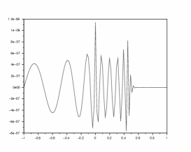
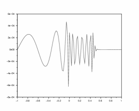
Figure 1. Test 1, final state for $\alpha=0.8$ (left) and $\alpha=1.2$ (right).

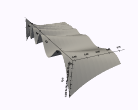
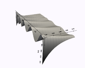
Figure 2. Test 1, control $h(x,t)$ for $\alpha=0.8$ (left) and $\alpha=1.2$ (right). The scaling factor is respectively $10^{-5}$ and $2\cdot 10^{-8}$.

Example 2.

In the second numerical example, the initial state is supported in ${\mathbb{R}}_{+}$, and more precisely

(8.12) $$u_{0}(x)=\chi_{(1/4,1/2)},$$

which results in a zero-controllable state for all values of $\alpha$. The results are shown in Figg. 3–4, for both $\alpha=0.8$ (left) and $\alpha=1.2$ (right), where the plots of $h$ have been scaled by a factor of respectively $5\cdot 10^{-4}$ for $\alpha=0.8$ and $5\cdot 10^{-5}$ for $\alpha=1.2$.

In this case, the initial state is controllable and the scales are similar: the final state has an $L^{2}$ norm of about $6\cdot 10^{-9}$ for $\alpha=0.8$ and about $10^{-7}$ for $\alpha=1.2$, according to the theoretical prediction. Note that, since the initial state is symmetric to that of Example 1, in both cases we would have the same final norm for the uncontrolled state equation.

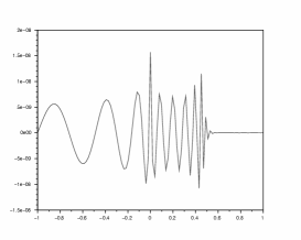
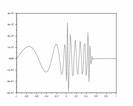
Figure 3. Test 2, final state for $\alpha=0.8$ (left) and $\alpha=1.2$ (right).

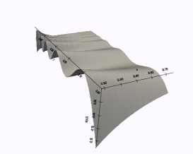
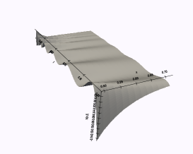
Figure 4. Test 2, control $h(x,t)$ for $\alpha=0.8$ (left) and $\alpha=1.2$ (right). The scaling factor is respectively $5\cdot 10^{-4}$ and $5\cdot 10^{-5}$.

As a final remark, we note that the agreement between theory and numerics must be understood in a qualitative form: numerical tests show that the value $\alpha=1$ works as a threshold between controllable and non-controllable situations. However, in the numerical setting under consideration the transition between the two cases appears to be continuous, and the influence of degeneracy on the null controllability of the discrete system is definitely worth a deeper investigation.

References

- [1] F. Alabau-Boussouira, P. Cannarsa and G. Fragnelli, Carleman estimates for degenerate parabolic operators with applications to null controllability, J. evol. equ. 6 (2006).
- [2] F. Ammar Khodja, A. Benabdallah, M. González-Burgos, L. de Teresa, The Kalman condition for the boundary controllability of coupled parabolic systems. Bounds on biorthogonal families to complex matrix exponentials, J. Math. Pures Appl. 96 (2011), p. 555-590.
- [3] A. Benabdallah, F. Boyer, M. González-Burgos, G. Olive, Sharp estimates of the one-dimensional boundary control cost for parabolic systems and applications to the -dimensional boundary null controllability in cylindrical domains, SIAM J. Control Optim., Vol. 52, No. 5, pp. 2970-3001.
- [4] K. Beauchard, P. Cannarsa, Heat equation on the Heisenberg group: observability and applications, J. Differ. Equations 262 (2017), no. 8, 4475–4521.
- [5] K. Beauchard, P. Cannarsa, R. Guglielmi,Null controllability of Grushin-type operators in dimension two, J. Eur. Math. Soc. (JEMS) 16 (2014), No. 1, 67-101.
- [6] K. Beauchard, P. Cannarsa, M. Yamamoto, Inverse source problem and null controllability for multidimensional parabolic operators of Grushin type, Inverse Probl. 30 (2014), no. 2, 26 pp.
- [7] K. Beauchard, L. Miller, M. Morancey, 2D Grushin-type equations: minimal time and null controllable data, J. Differential Equations. 259 (11), 2015.
- [8] F. Black, M. Scholes, The pricing of options and corporate liabilities, J. Polit. Econ. 81 (1973), no. 3, 637–654.
- [9] F. Boyer, F. Hubert and J. Le Rousseau, Discrete Carleman estimates for elliptic operators and uniform controllability of semi-discretized parabolic equations, J. Math. Pures Appl. 93 (2010) 240–276.
- [10] F. Boyer, F. Hubert and J. Le Rousseau, Uniform null-controllability properties for space/time-discretized parabolic equations, Num. Math. 118 (2011) 601–661.
- [11] H. Brezis, Analyse fonctionelle, Théorie et applications, Collection of Applied Mathematics for the Master’s degree, Masson, Paris, 1983.
- [12] M. I. Budyko, On the origin of glacial epochs, Meteor. Gidrol. 2 (1968), 3–8.
- [13] M. I. Budyko, The effect of solar radiation variations on the climate of the earth, Tellus 21 (1969), 611–619.
- [14] M. Campiti, G. Metafune, D. Pallara, Degenerate self-adjoint evolution equations on the unit interval, Semigroup Forum, 57, (1998), 1-36.
- [15] P. Cannarsa, G. Fragnelli, D. Rocchetti, Null controllability of degenerate parabolic operators with drift, Netw. Heterog. Media 2 (2007), no. 4, 695–715.
- [16] P. Cannarsa, P. Martinez, J. Vancostenoble, Null Controllability of degenerate heat equations, Adv. Differential Equations 10 (2005), 2, 153-190.
- [17] P. Cannarsa, P. Martinez, J. Vancostenoble, Carleman estimates for a class of degenerate parabolic operators, SIAM J. Control Optim. 47, (2008), no. 1, 1–19.
- [18] P. Cannarsa, P. Martinez, J. Vancostenoble, Global Carleman estimates for degenerate parabolic operators with applications, Memoirs of the American Mathematical Society (2016), Vol. 239.
- [19] P. Cannarsa, P. Martinez, J. Vancostenoble, The cost of controlling weakly degenerate parabolic equations by boundary controls, Math. Control Relat. Fields (2017), Vol 7, No 2, p. 171-211.
- [20] P. Cannarsa, P. Martinez, J. Vancostenoble, The cost of controlling strongly degenerate equations, ESAIM COCV, to appear.
- [21] P. Cannarsa, D. Rocchetti, J. Vancostenoble, Generation of analytic semi-groups in for a class of second order degenerate elliptic operators, Control Control and Cybernetics, vol. 37 (2008) No. 4
- [22] J.M. Coron, S. Guerrero, Singular optimal control: A linear 1-D parabolic-hyperbolic example, Asymp. Anal. 44, No 3-4, (2005), p. 237-257.
- [23] J.I. Díaz, On the mathematical treatment of energy balance climate models. The mathematics of models for climatology and environment, (Puerto de la Cruz, 1995), 217–251, NATO ASI Ser. Ser. I Glob. Environ. Change, 48, Springer, Berlin, 1997.
- [24] S. Ervedoza, E. Zuazua, Sharp observability estimates for heat equations, Arch. Ration. Mech. Anal. 202, No 3, 975-1017.
- [25] L. Escauriaza, G. Seregin, V. Šverák, Backward uniqueness for the heat operator in half-space, St. Petersburg Math. J. 15 (2004), no. 1, 139–148.
- [26] T. Ethier, A class of degenerate diffusion processes occurring in population genetics, Comm. Pure Appl. Math. 29 (1976), no. 5, 483–493.
- [27] T. Ethier, Fleming-Viot processes in population genetics, SIAM J. Control Optim. 31 (1993), no. 2, 345–386.
- [28] W.N. Everitt, A catalogue of Sturm-Liouville differential equations, Sturm-Liouville Theory, 271-331, Birkhäuser, Basel (2005).
- [29] H. O. Fattorini, D. L. Russel, Exact Controllability Theorems for Linear Parabolic Equations in One Space Dimension, Arch. Rat. Mech. Anal. 4, 272-292 (1971).
- [30] H. O. Fattorini, D. L. Russel, Uniform bounds on biorthogonal functions for real exponentials with an application to the control theory of parabolic equations, Quart. Appl. Math. 32 (1974/75), 45-69.
- [31] E. Fernandez-Cara, E. Zuazua, The cost of approximate controllability for heat equations: the linear case, Adv. Differential equations 5 (2000), No 4-6, 465-514.
- [32] G. Fragnelli, D. Mugnai, Carleman estimates, observability inequalities and null controllability for interior degenerate non smooth parabolic equations, Mem. Amer. Math. Soc. 242 (2016), No. 1146.
- [33] G. Fragnelli, D. Mugnai, Carleman estimates for singular parabolic equations with interior degeneracy and non smooth coefficients, Adv. Nonlinear Anal. 6 (2017), No 1, p. 61-84.
- [34] A. V. Fursikov, O. Yu. Imanuvilov, Controllability of evolution equations. Lecture Notes Ser. 34, Seoul National University, Seoul, Korea, 1996.
- [35] M. Ghil, Climate stability for a Sellers type model, Journal of the Atmospheric Sciences 33 (1976), no. 1, 3–20.
- [36] O. Glass, A complex-analytic approach to the problem of uniform controllability of transport equation in the vanishing viscosity limit, J. Funct. Anal. 258 (2010), No 3, p. 852-868.
- [37] S. Guerrero, G. Lebeau, Singular optimal control for a transport-diffusion equation, Communications in Partial Differential Equations 32 (2007), no. 10-12, 18, 1813–1836.
- [38] M. Gueye, Exact boundary controllability of 1-D parabolic and hyperbolic degenerate equations, SIAM J. Control Optim. 52 (2014), No 4, p. 2037-2054.
- [39] E.N. Güichal, A lower bound of the norm of the control operator for the heat equation, Journal of Mathematical Analysis and Applications 110 (1985), p. 519-527.
- [40] S. Hansen, Bounds on functions biorthogonal to sets of complex exponentials; control of damped elastic systems, Journal of Math. Anal. and Appl., 158 (1991), 487-508.
- [41] E. Kamke, Differentialgleichungen: Lösungsmethoden und Lösungen. Band 1: Gewöhnliche Differentialgleichungen. 3rd edition, Chelsea Publishing Company, New York, 1948.
- [42] V. Komornik, P. Loreti, Fourier Series in Control Theory, Springer, Berlin, 2005.
- [43] S. Labbé, E. Trelat, Uniform controllability of semidiscrete approximations of parabolic control systems, Syst. & Contr. Lett. 55 (2006), 597–609.
- [44] J. Lagnese, Control of wave processes with distributed controls supported on a subregion, SIAM J. Control Optim. 21 (1983), no. 1, 68-85.
- [45] G. Lebeau, L. Robbiano, Contrôle exact de l’équation de la chaleur, Comm. Partial Differential Equations 20 (1995), p. 335-356.
- [46] N.N. Lebedev, Special Functions and their Applications, Dover Publications, New York, 1972
- [47] J.-L. Lions, Exact controllability, stabilization and perturbations for distributed systems, SIAM Rev. 30 (1988), 1–68.
- [48] P. Lissy, On the cost of fast controls for some families of dispersive or parabolic equations in one space dimension, SIAM J. Control Optim. 52 (2014), no. 4, 2651–2676.
- [49] P. Lissy, Explicit lower bounds for the cost of fast controls for some 1-D parabolic or dispersive equations, and a new lower bound concerning the uniform controllability of the 1-D transport-diffusion equation, J. Differential Equations 259 (2015), no. 10, 5331–5352.
- [50] A. Lopez, E. Zuazua, Some new results related to the null controllability of the 1-d heat equation, Sém. EDP, Ecole Polytechnique, VIII, (1998), 1–22.
- [51] L. Lorch, M.E. Muldoon, Monotonic sequences related to zeros of Bessel functions, Numer. Algor (2008) 49, p. 221-233.
- [52] G. Citti, M. Manfredini, A degenerate parabolic equation arising in image processing, Commun. Appl. Anal. 8 (2004), no, 1, 125–141.
- [53] P. Martin, L. Rosier, P. Rouchon, Null controllability of the 1D heat equation using flatness, Proceedings of the 1st IFAC Workshop on Control of Systems Governed by Partial Differential Equations (CPDE2013), 2013, pp. 7-12.
- [54] P. Martin, L. Rosier, P. Rouchon, Null controllability of the heat equation using flatness, Automatica J. IFAC, 50 (2014), pp. 3067-3076.
- [55] P. Martin, L. Rosier, P. Rouchon, Null controllability of one-dimensional parabolic equations by the flatness approach, SIAM J. Control Optim. Vol 54, No 1 (2016), p. 198-220.
- [56] P. Martinez, J. Vancostenoble, Carleman estimates for one-dimensional degenerate heat equations. J. Evol. Eq 6 (2006), no. 2, 325–362.
- [57] L. Miller, Geometric bounds on the growth rate of null-controllability cost for the heat equation in small time, J. Differential Equations 204 (2004), No 1, p. 202-226.
- [58] L. Miller, The control transmutation method and the cost of fast controls, SIAM J. Control Optim. 45 (2006) 762–772.
- [59] I. Moyano, Flatness for a strongly degenerate 1-D parabolic equation, Math. Control Signals Syst. 28, No 4, paper No 28, 22p (2016).
- [60] Y. Privat, E. Trélat and E. Zuazua, Optimal observation of the one-dimensional wave equation, J. Fourier Anal. Appl., 19(2013), 514-544.
- [61] R.M. Redheffer, Elementary remarks on completeness, Duke Math. Journal 35 (1968), p. 103-116.
- [62] L. Schwartz, Étude des sommes d’exponentielles, deuxième édition. Paris, Hermann 1959.
- [63] T.I. Seidman, Two results on exact boundary control of parabolic equations, Appl. Math. Optim. 11 (1984), No 2, p. 145-152.
- [64] T.I. Seidman, S.A. Avdonin, S.A. Ivanov, The ”window problem” for series of complex exponentials, J. Fourier Anal. Appl. 6 (2000),No 3, p. 233-254.
- [65] W. D. Sellers, A climate model based on the energy balance of the earth-atmosphere system, J. Appl. Meteor. 8 (1969), 392–400.
- [66] V. Thomée, Galerkin Finite Element Methods for Parabolic Problems, Springer–Verlag, Heidelberg, 2006.
- [67] G. Tenenbaum, M. Tucsnak, New blow-up rates for fast controls of Schrodinger and heat equations, J. Differential Equations 243 (2007), p. 70-100.
- [68] G. Tenenbaum, M. Tucsnak, On the null controllability of diffusion equations, ESAIM: COCV 17 (2011) 1088–1100.
- [69] G. N. Watson, A treatise on the theory of Bessel functions, second edition, Cambridge University Press, Cambridge, England, 1944.
- [70] X. Zhang, E. Zuazua, Long-time behavior of a coupled heat-wave system arising in fluid-structure interaction, Arch. Ration. Mech. Anal. 184 (2007), No. 1, p. 49-120.