Intra-cell dynamics and cyclotron motion without magnetic field

Abstract

Intra-cell motion endows rich non-trivial phenomena to a wide variety of quantum materials. The most prominent example is a transverse current in the absence of a magnetic field (i.e. the anomalous Hall effect). Here we show that, in addition to a dc Hall effect, anomalous Hall materials possess circulating currents and cyclotron motion without magnetic field. These are generated from the intricate wavefunction dynamics within the unit cell, and correspond to interband transitions (coherences) in much the same way that cyclotron resonances arise from inter-Landau level transitions in magneto-optics. Curiously, anomalous cyclotron motion exhibits an intrinsic decay in time (even in pristine materials) displaying a characteristic power law decay. This reveals an intrinsic dephasing similar to that of inhomogeneous broadening of spinors. Circulating currents can manifest as the emission of circularly polarized light pulses in response to incident linearly polarized (pulsed) electric field, and provide a direct means of interrogating the intra-unit-cell dynamics of quantum materials.

In crystals with a multi-basis unit cell (multiple atoms/orbitals), the weight of the wavefunction on each basis plays a non-trivial role in the long wavelength dynamics of electrons. An illustrative example is graphene where a pseudo-spin arises from the relative wavefunction amplitude and phase on A and B sublattice sites within the unit cell: these define an intra-(unit) cell coordinate. This pseudo-spin is instrumental in a variety of Berry-phase related electronic phenomena that range from Klein tunneling katsnelson06 to a pinned zeroth Landau level novoselov04 ; novoselov05 ; pkim05 . Non-trivial internal structure within the unit cell arises across a variety of multi-band quantum materials where geometric phases transform particle motion.

Perhaps the most striking consequence of non-trivial intra-cell coordinate motion is the anomalous Hall effect (AHE), in which transverse currents can be induced by a longitudinal electric field even in the absence of a magnetic field adams59 ; luttinger54 ; niu99 ; xiao10 . Although the average position of electron wavepackets in a crystal is ambiguous and depends on a gauge choice, intra-cell displacements, on the other hand, are gauge invariant quantities. In anomalous Hall materials, the non-trivial structure of intra-cell coordinates render the components of the physical position operator/coordinate non-commuting adams59 . This results in an anomalous velocity (AV) transverse to the applied electric field in the semiclassical equations of motion for particles adams59 ; luttinger54 ; niu99 ; xiao10 .

Here, we show that in addition to a slow transverse drift arising from AV, anomalous Hall materials exhibit unusual intra-cell dynamics with a characteristic anomalous cyclotron-like motion without magnetic field. For example, focussing on a prototypical anomalous Hall material – a broken time reversal symmetry (TRS) gapped Dirac system with two sites per unit cell – we find that the probability to find an electron on either A or B sites (wavefunction square amplitude) can naturally oscillate between the sites (Fig. 1a). This unusual intra-cell oscillator leads to a real-space cyclotron motion (of the entire electron liquid) even when the valence band is fully occupied. The anomalous cyclotron motion (ACM) can be activated by either applying a short electric pulse (Fig. 2) or rapidly turning on an electric field (Fig. 3). Both approaches induce cyclotron currents that can be probed via emission of circularly polarized light when linearly polarized fields are incident on a sample ( Figs. 4).

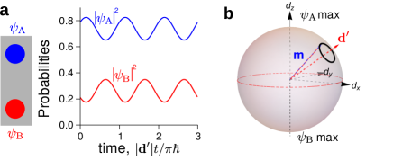
Figure 1: Intra-cell dynamics. a. Weight of wave function $\psi_{A},\psi_{B}$ on two sites of a unit cell can be modulated by an external electric field $E_{x}^{\delta}\delta(t)\hat{{\bf x}}$. Here ${\bf d}^{\prime}=(d_{x}+evE_{x}^{\delta},d_{y},d_{z})$. b. The wave function is related to a pseudo-spinor, ${\bf m}=\langle\psi({\bf p})|\boldsymbol{\tau}|\psi({\bf p})\rangle$, where $\boldsymbol{\tau}_{x,y,z}$ are Pauli matrices, see text. Pseudo-spinor ${\bf m}$ (blue dashed line) is initially aligned to ${\bf d}$. When an electric field pulse $E_{x}^{\delta}\delta(t)\hat{{\bf x}}$ is applied, ${\bf d}$ is displaced to ${\bf d}^{\prime}$. As a result, ${\bf m}$ precesses around ${\bf d}^{\prime}$. North (south) pole of Bloch sphere indicates a state where $|\psi_{\rm A}|^{2}=1$ ($|\psi_{\rm B}|^{2}=1$). Here we have used $d_{x}=d_{y}=d_{z}=\Delta$ and a small electric field pulse amplitude.

Similar to how slow guiding center motion (Hall drift) and fast cyclotron motion in the presence of a magnetic field are dual to each other, the slow transverse drift from semiclassical AV in anomalous Hall materials possesses an analogous duality to the fast ACM we describe here. This is because both ACM and AV arise from the same origin — a non-trivial quantum geometry in the Bloch bands encoded in the intra-cell coordinate structure. To see this, we recall that AV arises from the adiabatic motion of carriers projected onto a single band. In contrast, ACM arises from the non-adiabatic dynamics of carriers and corresponds to inter-band transitions between the bands. This is similar to the relationship between magnetic field induced guiding center motion and cyclotron motion which can be understood as arising from the motion of carriers projected to a single Landau level and virtual transitions between Landau levels respectively. Much as cyclotron motion encodes the dynamical response found in magneto-optics, ACM is the physical manifestation of the dynamical response of anomalous Hall materials mcd10 ; levitov11 ; brey14 ; rostami14 ; carbotte17 .

However, in contrast to conventional cyclotron motion in a magnetic field, the ACM we discuss here exhibits intrinsic $1/t$ power-law decay, even in a pristine and intrinsic system. This decay arises from dephasing due to inhomogeneous broadening of the pseudo-spinors (in-momentum space). When electric field is applied, pseudo-spinors in different states exhibit multi-frequency Larmor precession (each pseudo-spinor precesses with a different frequency and direction) thus creating dephasing. Nevertheless, the response is peaked for transitions close to the band edges, and displays a characteristic frequency that is tunable by the band gap in a massive Dirac system.

We begin by considering a system with two sites in a unit cell, thus having two bands. These two sites can correspond to two types of atoms or orbitals within the unit cell; this two-band model is the simplest system exhibiting a non-trivial intra-cell structure. We write the Hamiltonian as: $\mathcal{H}=\boldsymbol{\tau}\cdot{\bf d}({\bf p})$, where $\boldsymbol{\tau}_{x,y,z}$ are Pauli matrices that act on the sublattice A and B sites, ${\bf d}({\bf p})$ describes the band structure of the specific material, and ${\bf p}$ is the quasi-momentum. Intra-cell dynamics are encoded in the pseudo-spinor ${\bf m}_{{\bf p}}=\langle\psi({\bf p})|\boldsymbol{\tau}|\psi({\bf p})\rangle$, with $\psi({\bf p})=(\psi_{A}({\bf p}),\psi_{B}({\bf p}))$ which compactly describes amplitudes and phases of the electron wavefunction on the A and B sites. The dynamics of ${\bf m}_{{\bf p}}$ thus represent intra-cell motion that can be tracked in the Bloch sphere as illustrated in Fig. 1b. When ${\bf m}_{{\bf p}}$ is aligned to the north (south) pole of the Bloch sphere, the wave function has weight solely on A (B) sublattice.

Importantly, the pseudo-spinors obey the Bloch equation of motion

$$\frac{d}{dt}{\bf m}_{{\bf p}}(t)=\langle\psi({\bf p})|\frac{1}{i\hbar}[\boldsymbol{\tau},\mathcal{H}]|\psi({\bf p})\rangle=\frac{2}{\hbar}{\bf d}({\bf p})\times{\bf m}_{{\bf p}}.$$ (1)

At equilibrium (no applied electric field), ${\bf m}_{{\bf p}}={\bf m}^{(0)}_{{\bf p}}=\pm{\bf d}({\bf p})/|{\bf d}({\bf p})|$ corresponding to the pseudo-spinors of conduction and valence band states respectively. At equilibrium, conduction (valence) band pseudo-spinors ${\bf m}^{(0)}_{{\bf p}}$ are parallel (anti-parallel) to ${\bf d}({\bf p})$ yielding $d{\bf m}_{{\bf p}}/dt$ that vanishes. When an external electric field is applied, ${\bf d}$ is shifted by $\delta{\bf d}={\bf A}\partial_{\bf A}{\bf d}({\bf p}-e{\bf A}/c)$ to linear order. Here ${\bf A}$ is the vector potential, related to electric field by ${\bf E}=-\partial_{t}{\bf A}/c$. As a result, ${\bf m}_{\bf p}$ and ${\bf d}^{\prime}={\bf d}({\bf p}-e{\bf A}/c)$ are no longer aligned, turning on the dynamics of ${\bf m}_{\bf p}$.

The rate of change of the pseudo-spinor, $d{\bf m}_{{\bf p}}/dt$, is perpendicular to ${\bf m}_{{\bf p}}$ (see Eq. (S-3)) which makes the pseudo-spinor ${\bf m}_{{\bf p}}$ Larmor precesses around ${\bf d}^{\prime}$ similar to spin dynamics (see Fig. 1 b); this occurs naturally whenever ${\bf m}_{{\bf p}}$ is canted away from ${\bf d}({\bf p})$. This dynamics can be visualized as an oscillation of probability at each site (see Fig. 1a). As we will see, it is this intra-cell oscillation that leads to the unusual ACM we describe below. In the following we will capture the dynamics by writing ${\bf m}_{{\bf p}}(t)={\bf m}^{(0)}_{{\bf p}}+\delta{\bf m}_{{\bf p}}(t)$. We note that Eq. (S-3) can be nonlinear since $\delta{\bf m}$ and $\delta{\bf d}$ are both proportional to ${\bf E}$. In this work, however, we focus on linear response while leaving non-linear effects as a subject of further study.

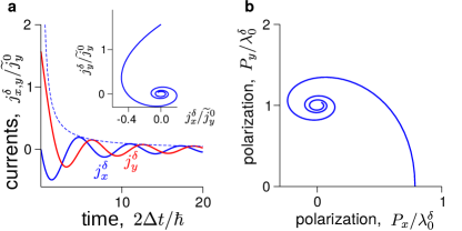
Figure 2: Anomalous cyclotron motion. a. In the presence of a linearly polarized pulse, $E_{x}^{\delta}\delta(t)\hat{{\bf x}}$, longitudinal current $j_{x}^{\delta}$ (blue line) and Hall current $j_{y}^{\delta}$ (red line) oscillate as a function of time. For $j_{y}^{\delta}$ plotted here, we have used $\chi=1$. Dashed line indicates $1/t$ decay. Here $\widetilde{j}_{y}^{0}=E_{x}^{\delta}\sigma_{H}2\Delta/\hbar$ and $\sigma_{H}=e^{2}/2h$. [Inset] $j_{x}^{\delta}$ vs $j_{y}^{\delta}$ are $\pi/2$ out-of-phase leading to a macroscopic circulating current. b. Polarization exhibits an initial shift in $x$ due to the pulse. It subsequently spirals inward displaying a macroscopic (real-space) cyclotron motion of charge carriers in anomalous Hall materials. This is obtained from integrating ${\bf j}^{\delta}$ over time (see text) where $\lambda_{0}^{\delta}=\sigma_{H}E_{x}^{\delta}$.

To understand the intra-cell dynamics in anomalous Hall materials, we specialize to TRS-broken gapped Dirac systems with ${\bf d}({\bf p})=(\chi vp_{x},vp_{y},\Delta)$ where $\chi=\pm 1$ is the chirality, $v$ is the Dirac velocity of electrons, and $\Delta$ is the energy difference between A and B sublattice sites. Since TRS is broken, we will focus on just a single cone. Although we focus on the simplest model, equivalent qualitative results can be drawn for different systems such as anomalous Hall ferromagnets, topological insulators, and Weyl and Dirac semimetals [see also below for a discussion of the half-Bernevig-Hughes-Zhang (half-BHZ) model].

As we now argue, the Larmor-like intra-cell motion (Fig. 1b) persists in the macroscopic dynamics of the entire electron liquid and manifests as ACM. To see this, we excite the system with linearly polarized light, ${\bf E}=E_{0}e^{-i\omega t}\hat{{\bf x}}$. Collecting the linear terms of Eq. (S-3), we obtain

$$\frac{d}{dt}\delta{\bf m}_{{\bf p}}(t)=\frac{2}{\hbar}\left({\bf d}({\bf p})\times\delta{\bf m}_{{\bf p}}(t)+\delta{\bf d}\times{\bf m}^{(0)}_{{\bf p}}\right),$$ (2)

where $\delta{\bf d}=i\chi evE_{0}/\omega\hat{{\bf x}}$. Here we have focussed on linear response, dropping the nonlinear term $\delta{\bf m}_{{\bf p}}\times\delta{\bf d}({\bf p})$. We note that the dynamics of $\delta{\bf m}_{\bf p}$ is controlled by the internal structure [the first term in the right hand side (RHS) of Eq. (S-4)], as well as the external driving [the second term in RHS of Eq. (S-4)]. The former gives rise to a precessional motion with frequency $2|{\bf d}|/\hbar$ that corresponds to the oscillation frequency of virtual interband transitions. We note, parenthetically, that this can be related to the trembling motion or Zitterbewegung of Dirac fermions katsnelson05 .

For a fully gapped system, with Fermi energy in the gap, the electrons are in the valence band. Solving for Fourier components $\delta{\bf m}\sim e^{-i\omega t}$ in Eq. (S-4), we obtain:

$$\delta m_{x}(\omega) = \frac{i\chi evE_{0}(d_{y}^{2}+d_{z}^{2})}{\omega|{\bf d}|((\hbar\omega/2)^{2}-|{\bf d}|^{2})},$$

$$\delta m_{y}(\omega) = \frac{-\chi evE_{0}\left((\hbar\omega/2)d_{z}+id_{x}d_{y}\right)}{\omega|{\bf d}|((\hbar\omega/2)^{2}-|{\bf d}|^{2})},$$

$$\delta m_{z}(\omega) = \frac{\chi evE_{0}\left((\hbar\omega/2)d_{y}-id_{x}d_{z}\right)}{\omega|{\bf d}|((\hbar\omega/2)^{2}-|{\bf d}|^{2})},$$ (3)

where we have used ${\bf m}^{(0)}_{{\bf p}}=-{\bf d}({\bf p})/|{\bf d}({\bf p})|$ corresponding to the valence band.

The current response of the entire electron liquid can be determined as ${\bf j}=e\sum_{{\bf p}}\langle\partial_{{\bf p}}\mathcal{H}\rangle=ev(\chi\sum_{{\bf p}}\delta m_{x},\sum_{\bf p}\delta m_{y},0)$, see supplementary information (SI) for a full account. Here the sum is taken over the entire valence band. We note that terms in Eq. (3) that are odd in $d_{x}$ and $d_{y}$ cancel during ${\bf p}$ integration. In the static limit $\omega\to 0$, the non-vanishing integrand of $\delta m_{y}$ reproduces the Berry curvature of gapped Dirac systems, $\chi v^{2}\hbar^{2}d_{z}/(2|{\bf d}|^{3})$; taking the integral of $\delta m_{y}$ over ${\bf p}$, one can obtain the (half) quantized Hall conductivity in the static limit expected from a single gapped Dirac cone per spin.

To demonstrate the full response of intra-cell dynamics, access to a broad range of frequency is needed. This can be achieved, for example, by an ultra short light pulse. For simplicity, we first consider the form ${\bf E}=E_{x}^{\delta}\delta(t)\hat{{\bf x}}$ (see SI for a Gaussian profile for a comparison). Using Eq. (3), the current that develops at $t>0$ in response to the delta function pulse is supplement :

$$j_{x}^{\delta}(t) =\frac{e^{2}}{4h}\frac{2\Delta E_{x}^{\delta}}{\hbar}\bigg{[}\tau\left({\rm Si}(\tau)-\frac{\pi}{2}\right)-\frac{{\rm sin}(\tau)}{\tau}$$

$$+\cos(\tau)+\pi\delta(\tau)\bigg{]},$$

$$j_{y}^{\delta}(t) =\frac{\chi e^{2}}{2h}\frac{2\Delta E_{x}^{\delta}}{\hbar}\left[\frac{\pi}{2}-{\rm Si}(\tau)\right],$$ (4)

where $\tau=2\Delta t/\hbar$, and ${\rm Si}(x)=\int_{0}^{x}dx^{\prime}\sin(x^{\prime})/x^{\prime}$. Here $j_{y}^{\delta}$ captures the dynamical anomalous Hall motion. The oscillatory motion of both $j_{x}^{\delta}$ (blue) and $j_{y}^{\delta}$ (red) with $\chi=1$ are shown explicitly in Fig. 2a. This oscillation (finite frequency response) indicates the contribution from virtual interband transitions.

Crucially, the oscillatory response of $j_{x}^{\delta}$ and $j_{y}^{\delta}$ are displaced in phase by $\pi/2$ and characterizes the ACM in gapped Dirac systems (Fig. 2a inset). The $\pi/2$ phase lag of $j_{y}^{\delta}$ vs $j_{x}^{\delta}$ is inherited from the intra-cell motion that leads to the Larmor preccession of the individual spinors in Fig. 1b. Indeed, the plot $j_{x}^{\delta}$ vs $j_{y}^{\delta}$ in the Inset of Fig. 2a shows a circulating current (ACM). The circulating current is centered at (0,0) because the delta-pulse electric field is (instantaneously) applied only at $t=0$.

To emphasize the real-space nature of ACM, we plot the change of polarization, $\Delta{\bf P}=\int_{0}^{t}{\bf j}(t^{\prime})dt^{\prime}$ shown in Fig. 2b. This demonstrates how the average displacement for the carriers circulates in a cyclotron fashion reminiscent of that found in the presence of a Lorentz force. This features a characteristic spiral pattern, picking out a handedness (determined by $\chi$) that describes the sense of rotation; broken TRS is integral to ACM .

We note, parenthetically, that before performing cyclotron motion (ACM), the carriers exhibit a (global) shift in position. Because of $\delta(\tau)$ in $j_{x}^{\delta}$ [see Eq. (4)], the electron liquid is initially displaced by $\pi\lambda_{0}^{\delta}/4$ and returns to equilibrium in the long time limit. Meanwhile in the $y$ direction, the electron liquid is polarized by an (electric-field-dependent) value $\chi\lambda_{0}^{\delta}$ where $\lambda_{0}^{\delta}=\sigma_{H}E_{x}^{\delta}$ and $\sigma_{H}=e^{2}/2h$ is the dc Hall conductivity for a single gapped Dirac cone per spin supplement . This can be understood by noting that, in the long time limit, polarization $\Delta{\bf P}$ from the delta function pulse is determined solely by the dc conductivity arising from intra-band contributions; we note that the inter-band contribution oscillates and its contribution to the polarization vanishes in the long time limit supplement . As a result, only a transverse polarization (arising from non-vanishing dc Hall conductivity) manifests at long times; longitudinal polarization diminishes to zero since dc longitudinal conductivity vanishes for a fully gapped system. This change of transverse polarization corresponds to the canting of ${\bf d}\to{\bf d}^{\prime}$ in Fig. 1b and appears due to the instantaneous drift induced by the delta function pulse field.

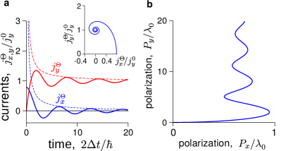
Figure 3: Coexistence of anomalous velocity and anomalous cyclotron motion. a. In the presence of a step function and homogeneous (in space) electric field $E_{x}^{\Theta}\hat{{\bf x}}$ at $t>0$, longitudinal current $j_{x}^{\Theta}$ (blue line) and Hall current $j_{y}^{\Theta}$ (red line) oscillate in time with a $\pi/2$ phase shift. For $j_{y}^{\Theta}$, we have selected $\chi=1$. Dashed lines indicate $1/t$ decay. Here $j_{y}^{0}=\sigma_{H}E_{x}^{\Theta}$ with $\sigma_{H}=e^{2}/2h$. [Inset] Current density spirals about $(j_{x}^{\Theta},j_{y}^{\Theta})=(0,1)j_{y}^{0}$ displaying ACM (circulating current) coexisting with AV ($j_{y}^{\Theta}=1$). b. Polarization of carriers obtained from integrating ${\bf j}^{\Theta}$ over time (see text). Here $\lambda_{0}=(\sigma_{H}/v)\lambda_{c}E_{x}^{\Theta}$ where $\lambda_{c}=\hbar v/2\Delta$ is the Compton wavelength.

In contrast to Larmor precession for a single ${\bf p}$ state in Fig. 1b, or to cyclotron motion in a magnetic field, the macroscopic ACM found in ${\bf j}^{\delta}$ deteriorates, and follows a power-law $1/t$ decay (see the dashed line in Fig. 2a). This decay can be understood as a dephasing arising due to inhomogeneous broadening. Whenever the electric field is applied, each pseudo-spinor at state ${\bf p}$ precesses with different frequency and direction. At very short times, all the spinors oscillate at the same time. However, after sometime they begin to oscillate out of phase and dephase. As a result, ACM (the sum total dynamics of all the spinors) decays. We note that this intrinsic decay can be slower than extrinsic scattering processes which may cut this slow-relaxation; nevertheless, the slow relaxation – that occurs even in the absence of extrinsic scattering – is a Hallmark of the non-trivial structure of the intra-cell coordinate dynamics.

Although the delta function pulse excites the entire frequency range ($\omega\in[0,\infty]$), the temporal profile of $j_{x}^{\delta}$ and $j_{y}^{\delta}$ predominantly follows an oscillation frequency $2\Delta/\hbar$. This corresponds to the bandgap (i.e. direct interband transition between band-edges) and is a physical manifestation of the sharp logarithmic resonance in ${\rm Re}\,[\sigma_{xy}(\omega)]$ and ${\rm Im}\,[\sigma_{xx}(\omega)]$ when $\omega$ matches with energy gap $2\Delta$ supplement ; mcd10 . This frequency further underscores the inter-band transition nature of ACM; the cyclotron-like intra-cell motion in these pulsed systems originate from inter-band wavefunction coherences induced by the pulse.

ACM (from inter-band coherence) can co-exist side-by-side with AV (from intra-band coherence). To see this, we apply a homogeneous electric field in space with a step function in time, $E_{x}^{\Theta}\Theta(t)\hat{{\bf x}}$, so as to get a dc response (corresponding to AV) as well as to incorporate a broad frequency range (to enable ACM discussed above). Using Eq. (3), we obtain the full current response at $t>0$ supplement :

$$j^{\Theta}_{x}(t) =\frac{e^{2}E_{x}^{\Theta}}{8h}\bigg{[}(\tau^{2}-2)\left({\rm Si}(\tau)-\frac{\pi}{2}\right)$$

$$+\tau\cos(\tau)+\sin(\tau)\bigg{]},$$

$$j_{y}^{\Theta}(t) =\frac{\chi e^{2}E_{x}^{\Theta}}{2h}\left[1-\cos(\tau)+\tau\left(\frac{\pi}{2}-{\rm Si}(\tau)\right)\right]$$ (5)

The step function (in time) and homogeneous (in space) field induces an oscillating response with frequency $2\Delta/\hbar$ in both $j_{x}^{\Theta}$ and $j_{y}^{\Theta}$ (blue and red lines, respectively in Fig. 3a).

The anomalous Hall current $j_{y}^{\Theta}$ for $\chi=1$ (red line of Fig. 3a) oscillates around $j_{y}^{0}=\sigma_{H}E_{x}^{\Theta}$. While $\sigma_{H}=e^{2}/2h$ arises from the intra-band part of the AHE, the full response we evaluate here modulates the Hall current and includes an inter-band contribution (that arises from the sharp turn-on).

Similar to ACM induced by a delta-function pulse (in Eq. (4) above), $j_{x}^{\Theta}$ and $j_{y}^{\Theta}$ decay as $1/t$ (dashed lines of Fig. 3a) and exhibits a phase lag of $\pi/2$. Plotting $j_{x}^{\Theta}$ vs $j_{y}^{\Theta}$ in the Inset of Fig. 3a, we display how ACM spirals inwards. We note that at long times this oscillation decays and approaches the value expected for adiabatic dc transport (i.e. a drift from AV); this is shown by the spiral that is centered around $j_{y}^{\Theta}=j_{y}^{0}$ indicating its long-time behavior. This shifted spiral indicates how ACM (most pronounced at short times) can co-exist with AV.

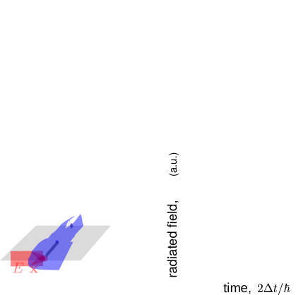
Figure 4: Circularly polarized light emission without magnetic field. a. A linearly polarized pulse $E_{x}^{\delta}\delta(t)\hat{{\bf x}}$ yields a circulating current ${\bf j}$ and circularly polarized light emission. b. Radiated electric field from cyclotron current in $x$ (blue line) and $y$ (red line) detected from a position ${\bf r}=(0,0,1)\ \mu{\rm m}$. We use $\chi=1$. [Inset] Evolution of radiated electric field polarization. c. Probing the intra-cell dynamics via emission of circular polarized light arising from a step function electric field $E_{x}^{\Theta}\Theta(t)\hat{{\bf x}}$. d. Radiated electric field in $x$ (blue line) and $y$ (red line) from ${\bf j}^{\Theta}$ with the same parameters as b. [Inset] Evolution of radiated electric field polarization. Jumps of $\boldsymbol{\mathcal{E}}$ at $t=|{\bf r}|/c$ are due to retardation.

For the step-function $E_{x}^{\Theta}\Theta(t)$, the predominant (real-space) displacement (polarization) is in the transverse direction ($y$ direction); it is accompanied by an oscillatory motion in $x$ (Fig. 3b). The oscillatory motion comes from the fact that $j_{x}^{\Theta}$ oscillates around zero (Fig. 3a). We note, parenthetically, there also exists a parallel translation in $x$ due to a non-zero integral of $j_{x}^{\Theta}$ over time. This translation is proportional to the applied electric field and $\Delta^{-1}$ as determined by a quantity $\lambda_{0}=(\sigma_{H}/v)\lambda_{c}E_{x}^{\Theta}$ where $\lambda_{c}=\hbar v/2\Delta$ is a Compton wavelength. For small gap $2\Delta=10$ meV, the Compton wavelength can be sizable, $\lambda_{c}=65$ nm. It corresponds to the build up of polarization along $x$.

Intra-cell dynamics can be probed by radiation of electromagnetic (EM) waves from the anomalous cyclotron current. Interestingly, these EM waves are circularly polarized even though the input pulse is linearly polarized, as illustrated in Figs. 4a and c. To illustrate this, we note that EM radiation from a current source is given by:

$$\boldsymbol{\mathcal{E}}({\bf r},t)=\frac{-1}{c^{2}}\int\frac{d^{3}{\bf r}^{\prime}}{|{\bf r}^{\prime}-{\bf r}|}\frac{d{\bf j}\left({\bf r}^{\prime},t-\frac{|{\bf r}^{\prime}-{\bf r}|}{c}\right)}{dt},$$ (6)

where $c$ is the speed of light. For the light pulse $E_{x}^{\delta}\delta(t)\hat{{\bf x}}$, we use a convenient choice for the laser spot size assuming it to be a circle with radius $1\ {\rm\mu m}$ for illustration. For the step function electric field $E_{x}^{\Theta}\Theta(t)\hat{{\bf x}}$, we assume homogeneous current density ${\bf j}^{\Theta}({\bf r},t)={\bf j}^{\Theta}(t)\delta(z)$ over an area of $1\ {\rm\mu m}^{2}$; other spot sizes can be chosen with no qualitative changes to the results we discuss below. The radiated electromagnetic waves $\boldsymbol{\mathcal{E}}^{\delta}$ and $\boldsymbol{\mathcal{E}}^{\Theta}$ are evaluated at a position ${\bf r}=1\ {\rm\mu m}\,\hat{{\bf z}}$ above the source as shown in Figs. 4b and d, respectively. Both $\boldsymbol{\mathcal{E}}^{\delta}$ and $\boldsymbol{\mathcal{E}}^{\Theta}$ decay following a power law $1/t$ and are circularly polarized (see Inset of Figs. 4b and d). The jumps of $\boldsymbol{\mathcal{E}}$ at $t=|{\bf r}|/c$ are due to the effect of retardation.

ACM is a generic phenomena that arises in a variety of other anomalous Hall materials. As a further example we consider the half Bernevig-Hughes-Zhang (BHZ) Hamiltonian with ${\bf d}^{\rm BHZ}=\left(\chi vp_{x},vp_{y},\Delta-m^{-1}(p_{x}^{2}+p_{y}^{2})\right)$; this has TRS explicitly broken. Here $m^{-1}$ is the inverse mass parameter. Using the same approach as above to tease out ACM, we apply a delta-function pulse $E_{x}^{\delta}\delta(t){\bf\hat{x}}$ and compare two cases of $m^{-1}=v^{2}/\Delta$ (solid lines) and $m^{-1}=0.1v^{2}/\Delta$ in Fig. 5. For both cases, $j_{x}$ and $j_{y}$ remain $\pi/2$ out-of-phase with each other. For small $m^{-1}$, the Hamiltonian tends to the same form as the Dirac system. As a result, the current response shows similar behaviour as compared to Fig. 2. For large $m^{-1}$, however, the amplitude of oscillation at long times is larger and lasts longer (with a smaller decay constant) than the gapped Dirac system analyzed above. Further. we note that $m^{-1}$ also modifies the oscillation frequency. Plotting $j_{x}$ vs $j_{y}$, we show circulating current that is long-lived exhibiting a sizable radius (Inset Fig. 5). As a result, for large $m^{-1}$, we expect thagt ACM in the BHZ-type systems is more pronounced compared to that found in massive/gapped Dirac systems (cf. Fig. 5b and Fig. 3b).

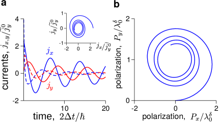
Figure 5: ACM of half-BHZ systems. a. Current response of a half-BHZ system (see text) when excited by a delta function pulse $E_{x}^{\delta}\delta(t){\bf\hat{x}}$. Longitudinal current $j_{x}$ (blue lines) and Hall current $j_{y}$ (red lines) are shown for two parameters $m^{-1}=v^{2}/\Delta$ (solid lines) and $m^{-1}=0.1v^{2}/\Delta$ (dashed lines) with $\chi=1$. [Inset] $j_{x}$ vs $j_{y}$ are $\pi/2$ out-of-phase leading to a macroscopic circulating current. b. Polarization of carriers show a a spiral-like character displaying a macroscopic (real-space) cyclotron motion. Here we used $m^{-1}=v^{2}/\Delta$ in Inset of a and in panel b.

In summary, we demonstrate how fast intra-cell dynamics can be tracked through a pulsed non-adiabatic excitation, manifesting in ACM without magnetic field. ACM can be found in a variety of anomalous Hall materials and display a number of unusual characteristics including an intrinsic power-law decay, and real-space charge displacements that follow a spiral-like trajectory. This can be easily tracked via circularly polarized emission induced by a linearly polarized pulsed excitation. Just as slow anomalous velocity of carriers characterizes the intra-band quantum geometry (e.g., Berry curvature) of anomalous Hall materials, ACM captures its inter-band coherences. Both of these are rooted in a non-trivial intra-unit-cell structure and constitute different aspects of Bloch band geometry; ACM provides a dynamical window into the inner (often hidden) dynamics within the unit cell.

Acknowledgements — We are grateful for useful conversations with Giovanni Viganle, Mark Rudner, Li-kun Shi, and Yang Bo. This work was supported by the Singapore National Research Foundation (NRF) under NRF fellowship award NRF-NRFF2016-05, and the Nanyang Technological University Singapore through a Start-up grant.

A. Intracell dynamics

In the following section, we will discuss intracell dynamics and its relation to cyclotron motion without magnetic field (anomalous cyclotron motion) in detail. To obtain the dynamics of the wavefunction within the unit cell it is useful to define the pseudospinors

$${\bf m}_{\bf p}=\langle\psi({\bf p})|\boldsymbol{\tau}|\psi({\bf p})\rangle,\quad\psi({\bf p})=(\psi_{A}({\bf p}),\psi_{B}({\bf p})),$$ (S-1)

where $\boldsymbol{\tau}_{x,y,z}$ are Pauli matrices that act on the sub-lattice $A$ and $B$ sites, with $\psi_{A},\psi_{B}\in C$ are the wavefunction values on each of the sites respectively, and ${\bf p}$ is momentum.

We will model the low-energy excitations (described by $\psi({\bf p})$) around each valley via a $2+1$ massive Dirac Hamiltonian

$$\mathcal{H}=\boldsymbol{\tau}\cdot{\bf d}({\bf p}),\quad{\bf d}({\bf p})=(\chi vp_{x},vp_{y},\Delta)$$ (S-2)

where $\chi$ is the chirality, $v$ is the Dirac velocity of the particles, and $\Delta$ the energy difference between $A$ and $B$ sublattice sites. Importantly, the pseudo-spinors obey the (Bloch) equations of motion

$$\frac{d{\bf m}_{\bf p}}{dt}=\langle\psi({\bf p})|\frac{1}{i\hbar}[\boldsymbol{\tau},\mathcal{H}]|\psi({\bf p})\rangle=-\frac{2}{\hbar}{\bf m}_{\bf p}\times{\bf d}({\bf p}).$$ (S-3)

We note that at equilibrium (no applied electric field), ${\bf m}_{{\bf p}}={\bf m}^{(0)}_{{\bf p}}=\pm{\bf d}({\bf p})/|{\bf d}({\bf p})|$ corresponding to the conduction and valence band states respectively. These pseudo-spinors of the conduction (valence) band states [at equilibrium] are parallel (anti-parallel) to ${\bf d}({\bf p})$ yielding $d{\bf m}_{{\bf p}}/dt$ that vanishes. However, as we discuss below, once an electric field is applied ${\bf d}$ cants turning on the dynamics of ${\bf m}_{{\bf p}}$.

Writing ${\bf m}_{\bf p}(t)={\bf m}_{\bf p}^{(0)}+\delta{\bf m}_{\bf p}(t)$, we solve for the linear response of the system:

$$\frac{d}{dt}\delta{\bf m}_{\bf p}=-\frac{2}{\hbar}\left(\delta{\bf m}_{\bf p}\times{\bf d}({\bf p})+{\bf m}_{\bf p}^{(0)}\times\delta{\bf d}\right),$$ (S-4)

where $\delta{\bf d}={\bf A}\partial_{\bf A}{\bf d}({\bf p}-e{\bf A}/c)$. We have dropped the nonlinear terms $\delta{\bf m}_{\bf p}\times\delta{\bf d}$. Without losing generality, we have also specialized to a linearly polarized electric field ${\bf E}=E_{x}e^{-i\omega t}\hat{{\bf x}}$. Inverting Eq. (S-4), we obtain $\delta{\bf m}$ directly as

$$\left(\begin{array}[]{c}\delta m_{x}\\ \delta m_{y}\\ \delta m_{z}\end{array}\right)=\frac{i\chi evE_{x}}{\omega f(\omega)}\left(\begin{array}[]{c c c}d_{x}^{2}-(\hbar\omega/2)^{2}&d_{x}d_{y}+id_{z}(\hbar\omega/2)&d_{x}d_{z}-id_{y}(\hbar\omega/2)\\ d_{x}d_{y}-id_{z}(\hbar\omega/2)&d_{y}^{2}-(\hbar\omega/2)^{2}&d_{y}d_{z}+id_{x}(\hbar\omega/2)\\ d_{x}d_{z}+id_{y}(\hbar\omega/2)&d_{y}d_{z}-id_{x}(\hbar\omega/2)&d_{z}^{2}-(\hbar\omega/2)^{2}\end{array}\right)\left(\begin{array}[]{c}0\\ d_{z}/|{\bf d}|\\ -d_{y}/|{\bf d}|\end{array}\right),$$ (S-5)

where $f(\omega)=i(\hbar\omega/2)\left((\hbar\omega/2)^{2}-|{\bf d}|^{2}\right)$. In obtaining the above, we have specialized to the dynamics valence band electrons, since the system we focus on in the main text is fully gapped with Fermi energy in the gap. In so doing we have used ${\bf m}^{(0)}_{{\bf p}}=-{\bf d}({\bf p})/|{\bf d}({\bf p})|$ corresponding to the spinors valence band. Writing out (S-5) explicitly we have

$$\delta m_{x} = \frac{i\chi evE_{x}(d_{z}^{2}+d_{y}^{2})}{g(\omega)}$$

$$\delta m_{y} = \frac{-\chi evE_{x}\left((\hbar\omega/2)d_{z}+id_{x}d_{y}\right)}{g(\omega)}$$

$$\delta m_{z} = \frac{\chi evE_{x}\left((\hbar\omega/2)d_{y}-id_{x}d_{z}\right)}{g(\omega)},$$ (S-6)

where $g(\omega)=\omega|{\bf d}|\left((\hbar\omega/2)^{2}-|{\bf d}|^{2}\right)$.

B. Longitudinal current

We now proceed to obtain the current dynamics, first focussing on frequency space. Longitudinal current of the entire electron liquid can be obtained directly from the pseudo-spinors above as

$$j_{x}(\omega)=e\sum_{\bf p}\langle\partial\mathcal{H}/\partial p_{x}\rangle=\chi ev\sum_{\bf p}\delta m_{x},$$ (S-7)

where the expectation value is taken for the valence band states by specifying ${\bf m}^{(0)}_{\bf p}=-{\bf d}({\bf p})/|{\bf d}({\bf p})|$ (see above) since we focus on a gapped Dirac system with Fermi energy in the gap. By using ${\bf j}(\omega)=\boldsymbol{\sigma}(\omega){\bf E}(\omega)$, we write the longitudinal conductivity as

$$\sigma_{xx}=\chi ev\sum_{\bf p}\frac{-i\chi ev(d_{z}^{2}+d_{y}^{2})}{\omega|{\bf d}|\left((\hbar\omega/2)^{2}-|{\bf d}|^{2}\right)}.$$ (S-8)

The real and imaginary parts of longitudinal conductivity can be obtained from the usual substitution $\omega\to\omega+i\eta$ where $\eta\to 0^{+}$. We note that the denominator of Eq. (S-8) can be decomposed into

$$\frac{1}{(\Omega+i\eta)^{2}-D^{2}}=\frac{1}{2D}\left(\frac{1}{\Omega+i\eta-D}-\frac{1}{\Omega+i\eta+D}\right).$$ (S-9)

Using Sokhotski-Plemelj relation

$${\rm lim}_{\eta\to 0+}\frac{1}{x\pm i\eta}={\rm p.v}\ \frac{1}{x}\mp i\pi\delta(x),$$ (S-10)

we directly obtain the real part of $\sigma_{xx}$ [1–4] as

$${\rm Re}\,\left[\sigma_{xx}(\omega)\right] = \frac{i4e^{2}v^{2}}{(2\pi\hbar)^{2}}\int_{p}\frac{pdpd\theta(d_{z}^{2}+d_{y}^{2})}{|{\bf d}|\omega}\frac{-i\pi\left(\delta(\hbar\omega-2|{\bf d}|)-\delta(\hbar\omega+2|{\bf d}|)\right)}{4|{\bf d}|},$$ (S-11)

$$= \frac{\pi e^{2}}{8h}\frac{\Omega^{2}+1}{\Omega^{2}}\Theta(|\Omega|-1),\quad\Omega=\frac{\hbar\omega}{2\Delta}.$$

We note that the explicit functional form of the real part of the conductivity alone is enough to determine the $t$-dynamics of current we focus on in the main text (see description below). However, for completeness, we also display the imaginary part of $\sigma_{xx}$ using this formulation. This can be obtained directly obtained from Eq. (S-11) via the Kramers-Kronig relations [1–4]:

$${\rm Im}\,\left[\sigma_{xx}(\omega)\right] = -\frac{1}{\pi}\int_{-\infty}^{\infty}\frac{{\rm Re}\,\left[\sigma_{xx}(\omega^{\prime})\right]}{\omega^{\prime}-\omega}d\omega^{\prime},$$ (S-14)

$$= \frac{-e^{2}}{4h}\left[\left(1+\frac{1}{\Omega^{2}}\right)\mathcal{S}(\Omega^{-1})-\frac{1}{\Omega}\right],\quad\mathcal{S}(x)=\bigg{\{}\begin{array}[]{c}{\rm acoth}(x),\quad x>1\\ {\rm atanh}(x),\quad x\leq 1\end{array},$$

where we have used the identity $\int dx\frac{x^{2}+1}{x^{2}(x-x_{0})}=\mathrm{ln}|x-x_{0}|\left(1+x_{0}^{-2}\right)-x_{0}^{-2}\mathrm{ln}|x|+(xx_{0})^{-1}$, and the relation $\mathcal{S}(x)=\frac{1}{2}\mathrm{ln}\left|\frac{x+1}{x-1}\right|$.

We now proceed to the $t$-dynamics central to the anomalous cyclotron motion discussed in the main text. Of particular interest, is the current dynamics that ensues after the application of a delta function pulse ${\bf E}(t)=E_{x}^{\delta}\delta(t)\hat{{\bf x}}$. This can be written as

$${\bf j}^{\delta}(t) = \frac{E_{x}^{\delta}\Theta(t)}{2\pi}\int_{-\infty}^{\infty}d\omega\left\{{\rm Re}\,\left[\boldsymbol{\sigma}(\omega)\right]+i{\rm Im}\,\left[\boldsymbol{\sigma}(\omega)\right]\right\}e^{-i\omega t},$$ (S-15)

$$= \frac{E_{x}^{\delta}\Theta(t)}{2\pi}\left\{\int_{-\infty}^{\infty}d\omega e^{-i\omega t}{\rm Re}\,\left[\boldsymbol{\sigma}(\omega)\right]+i\left(\frac{-1}{\pi}\right)\int_{-\infty}^{\infty}d\omega^{\prime}{\rm Re}\,\left[\boldsymbol{\sigma}(\omega^{\prime})\right]\int_{-\infty}^{\infty}d\omega\frac{e^{-i\omega t}}{\omega^{\prime}-\omega}\right\},$$

$$= \frac{2E_{x}^{\delta}\Theta(t)}{2\pi}\int_{-\infty}^{\infty}d\omega e^{-i\omega t}{\rm Re}\,[\boldsymbol{\sigma}(\omega)].$$

In obtaining Eq. (S-15), we transformed ${\rm Im}\,[\sigma_{xx}]$ and expressed it in terms of ${\rm Re}\,[\sigma_{xx}]$ via the Kramers-Kronig relation. We have also used the identity $\int_{-\infty}^{\infty}due^{-iut}/u=-i\pi{\rm sgn}\,(t)$.

Employing Eq. (S-15) and using Eq. (S-11) we have

$$j_{x}^{\delta}(t) = \frac{e^{2}}{4h}\frac{2\Delta E_{x}^{\delta}\Theta(t)}{\hbar}\left[\cos(\tau)+\tau\left({\rm Si}(\tau)-\frac{\pi}{2}\right)-{\rm sinc}(\tau)+\pi\delta(\tau)\right],\quad\tau=\frac{2\Delta t}{\hbar},$$ (S-16)

The first two terms in Eq. (S-16) come from $\int_{1}^{\infty}d\Omega\cos(\Omega\tau)/\Omega^{2}$, and we have used identities ${\rm Si}(x)=\int_{0}^{x}dy\ \mathrm{sinc}(y)$ and $\int_{0}^{\infty}dy\ \mathrm{sinc}(y)=\frac{\pi}{2}$, with $\mathrm{sinc}(y)=\sin(y)/y$. The two last terms come from the Fourier transform of the inverse top-hat function $\Theta(|\Omega|-1)$. The inverse top-hat function ensures a zero ${\rm Re}\,[\sigma_{xx}]$ when $|\hbar\omega|$ is below the gap size $2\Delta$ and a finite value when $|\hbar\omega|>2\Delta$. Because $\Theta(|\Omega|-1)$ is an even function, the integral yields $\rm sinc(\tau)$. The delta function $\delta(\tau)$ appears due to finite Dirac conductivity (${\rm Re}\,[\sigma_{xx}]$) at $\omega\to\infty$. This delta function $\delta(\tau)$ is responsible for the initial shift of the average carrier position as we integrate $j_{x}(t)$ over time (see Fig. 2b in the main text). We note that the functions $\cos(\tau)+\tau(\mathrm{Si}(\tau)-\pi/2)$ as well as $-{\rm sinc}(\tau)$ oscillate with envelopes that decay as $1/\tau$. As a result, $j_{x}^{\delta}$ is an oscillating function that decays as $1/\tau$.

Next, we discuss the case of a homogeneous electric field (in space) and step function in time ${\bf E}(t)=E_{x}^{\Theta}\Theta(t)\hat{{\bf x}}$. The current response $j_{x}^{\Theta}$ is given by

$$j_{x}^{\Theta}(t) = \frac{E_{x}^{\Theta}}{2\pi}\int_{0}^{t}dt^{\prime}\int_{-\infty}^{\infty}d\omega\left\{{\rm Re}\,\left[\sigma_{xx}(\omega)\right]+i{\rm Im}\,\left[\sigma_{xx}(\omega)\right]\right\}e^{-i\omega(t-t^{\prime})}$$ (S-17)

$$= \frac{2E_{x}^{\Theta}}{2\pi}\Theta(t)\int_{-\infty}^{\infty}d\omega\frac{i(e^{-i\omega t}-1)}{\omega}{\rm Re}\,[\sigma_{xx}(\omega)],$$

$$= \frac{e^{2}E_{x}^{\Theta}\Theta(t)}{8h}\left[\sin(\tau)+\tau\left(\cos(\tau)+\tau\left({\rm Si}(\tau)-\frac{\pi}{2}\right)\right)-2\left({\rm Si}(\tau)-\frac{\pi}{2}\right)\right],\quad\tau=\frac{2\Delta t}{\hbar},$$

where $\tau$ is a dimensionless time. Here we have expressed ${\rm Im}\,[\sigma_{xx}]$ into ${\rm Re}\,[\sigma_{xx}]$ via Kramers-Kronig relation similar to Eq. (S-15). The first two terms come from integration by parts, $2\int_{1}^{\infty}d\Omega\frac{\sin(\Omega\tau)}{\Omega^{3}}=\sin(\tau)+\tau\int_{1}^{\infty}\frac{\cos(\Omega\tau)}{\Omega^{2}}$ while the last terms come from usual sine integral $\int_{\tau}^{\infty}dx\ \mathrm{sinc}(x)=\frac{\pi}{2}-\mathrm{Si}(\tau)$. The combined contribution of the first two terms as well as the last term are oscillating functions with envelopes that decay as $1/\tau$. As a result, $j_{x}^{\Theta}$ is an oscillating function that decays as $1/\tau$.

C. Anomalous Hall current

We now turn to the anomalous Hall current $j_{y}$ which can be evaluated as

$$j_{y}(\omega)=ev\sum_{\bf p}\delta m_{y},$$ (S-18)

where the summation p is taken for the valence band states. From this we obtain the real part of anomalous Hall conductivity [1–3],

$${\rm Re}\,[\sigma_{xy}(\omega)] = \frac{-\chi e^{2}v^{2}}{\omega}\sum_{\bf p}\frac{(\hbar\omega/2)d_{z}+id_{x}d_{y}}{((\hbar\omega/2)^{2}-|{\bf d}|^{2})|{\bf d}|},$$ (S-21)

$$= \frac{\chi e^{2}}{2h}\frac{1}{\Omega}\mathcal{S}(\Omega^{-1}),\quad\mathcal{S}(x)=\bigg{\{}\begin{array}[]{c}{\rm acoth}(x),\quad x>1\\ {\rm atanh}(x),\quad x\leq 1\end{array},$$

where $\Omega=\frac{\hbar\omega}{2\Delta}$ and we have used the identity $\int_{1}^{\infty}\frac{dx}{a^{2}-x^{2}}=-\frac{1}{a}\mathcal{S}(a^{-1})$. At $\omega\to 0$, $\sigma_{xy}$ shows a half-quantized value $e^{2}/2h$ for a single gapped Dirac cone. This transverse motion is non-dissipative since it arises from an undergap intraband contribution. At finite $\omega$, $\sigma_{xy}(\omega)$ is peaked at $\hbar\omega=2\Delta$ showing a logarithmic resonance; it subsequently decreases for $\hbar\omega>2\Delta$. This resonant behaviour is a signature of virtual interband transition.

For the imaginary part ${\rm Im}\,[\sigma_{xy}]$, we substitute $\omega\to\omega+i\eta$ and follow the same procedure as ${\rm Re}\,[\sigma_{xx}]$ to obtain [1–3]:

$${\rm Im}\,[\sigma_{xy}(\omega)]=\frac{-\chi e^{2}\pi}{4h}\frac{1}{\Omega}\Theta(|\Omega|-1).$$ (S-22)

The imaginary part of the anomalous Hall conductivity is dissipative response from interband transitions. We note that the real and imaginary parts of the Hall conductivity are related via Kramers-Kronig relations.

Next, we calculate the Hall response current for a delta function pulse ${\bf E}(t)=E_{x}^{\delta}\delta(t)\hat{{\bf x}}$. From the previous analysis in Eq. (S-15) above, we note that the contributions to the charge current $t$-dynamics from the real and imaginary parts of Hall conductivity are equal. As a result, we obtain

$$j_{y}^{\delta}(t) = 2\frac{E_{x}^{\delta}\Theta(t)}{2\pi}\int_{-\infty}^{\infty}d\omega{\rm Re}\,[\sigma_{xy}(\omega)]e^{-i\omega t}$$ (S-23)

$$= \frac{\chi e^{2}}{2h}\frac{2\Delta E_{x}^{\delta}\Theta(t)}{\hbar}\left[\frac{\pi}{2}-{\rm Si}(\tau)\right],$$

where we have used $\int_{-\infty}^{\infty}d\omega\frac{e^{-i\omega t}}{\omega^{2}-a^{2}}=-\frac{\pi}{a}\sin(at)$ and the usual sine integral $\int_{\tau}^{\infty}dx\ \mathrm{sinc}(x)=\frac{\pi}{2}-\mathrm{Si}(\tau)$. $j_{y}^{\delta}(t)$ is an oscillating function that decays as $1/t$. The current predominantly oscillates with frequency determined from the gap size $\omega=2\Delta/\hbar$ due to the logarithmic resonance of ${\rm Re}[\sigma_{xy}(\omega)]$.

We proceed to obtain the Hall current for homogeneous electric field in space and step function in time $E_{x}^{\Theta}\Theta(t)\hat{{\bf x}}$,

$$j_{y}^{\Theta}(t) = \frac{2E_{x}^{\Theta}}{2\pi}\int_{0}^{t}dt^{\prime}\int_{-\infty}^{\infty}d\omega{\rm Re}\,[\sigma_{xy}(\omega)]e^{-i\omega(t-t^{\prime})},$$ (S-24)

$$= \frac{\chi e^{2}E_{x}^{\Theta}}{2h}\Theta(t)\left(1-\tau\left({\rm Si}(\tau)-\frac{\pi}{2}\right)-\cos(\tau)\right),\quad\tau=\frac{2\Delta t}{\hbar}.$$

We have used an identity $\int_{-\infty}^{\infty}d\omega\frac{i(e^{-i\omega t}-1)}{\omega(\omega-a)(\omega+a)}=-\frac{\pi}{a^{2}}\left(\cos(at)-1\right)$ and $\int_{1}^{\infty}d\Omega\cos(\Omega\tau)/\Omega^{2}=\cos(\tau)+\tau\left({\rm Si}(\tau)-\frac{\pi}{2}\right)$ as obtained previously in Eq. (S-16). $j_{y}^{\Theta}$ shows an oscillating behavior that decays as $1/t$ from an interband contribution. The constant dc Hall current $e^{2}/2hE_{x}^{\Theta}$ arises from an intraband contribution.

D. Change of polarization in a delta function pulse

Electric polarization is defined by $\partial_{t}{\bf P}={\bf j}$. This can be seen by defining the polarization as $\nabla\cdot{\bf P}=-\rho$, where $\rho$ is charge density and taking the continuity equation $\nabla\cdot{\bf j}+\partial_{t}\rho=0$. In the case of a delta function pulse, the whole time integral of current response (polarization) is related to the dc conductivity. This can be seen directly from

$$\int dt{\bf j}^{\delta}(t) = \frac{2E_{x}^{\delta}}{2\pi}\int_{-\infty}^{\infty}dt\Theta(t)\int_{-\infty}^{\infty}d\omega{\rm Re}\,[\boldsymbol{\sigma}(\omega)]e^{-i\omega t},$$ (S-25)

$$= E_{x}^{\delta}{\rm Re}\,[\boldsymbol{\sigma}(0)],$$

In obtaining this, we have used the Fourier transform $\int_{-\infty}^{\infty}dte^{-i\omega t}\Theta(t)=\pi\delta(\omega)-i/\omega$ and noted that only the delta function $\delta(\omega)$ survives as ${\rm Re}\,[\boldsymbol{\sigma}(\omega)]/\omega$ is antisymmetric function that vanishes upon integration of $\omega$. Equation (S-25) suggests that, for a fully gapped system, only the Hall shift (polarization in $y$) is finite due to a quantized dc Hall conductivity $\sigma_{xy}(\omega=0)$.

E. Half Bernevig-Hughes-Zhang (BHZ) model

The half BHZ Hamiltonian has a ${\bf d}$ vector that follows ${\bf d}=(\chi vp_{x},vp_{y},\Delta-m^{-1}(p_{x}^{2}+p_{y}^{2}))$, where $m^{-1}$ is the inverse of the mass term. With applied electric field in the $x$ direction, $p_{x}\to p_{x}+ieE_{x}e^{-i\omega t}/\omega$, we have $\delta d_{x}=i\chi evE_{x}/\omega$ and $\delta d_{z}=-2i\chi em^{-1}p_{x}E_{x}/\omega$. We have dropped the nonlinear terms in ${\bf E}$ since we focus on linear response. Solving the linear equation (S-4), we obtain

$$\left(\begin{array}[]{c c c}-i\hbar\omega/2&d_{z}&-d_{y}\\ -d_{z}&-i\hbar\omega/2&d_{x}\\ d_{y}&-d_{x}&-i\hbar\omega/2\end{array}\right)\left(\begin{array}[]{c}\delta m_{x}\\ \delta m_{y}\\ \delta m_{z}\end{array}\right)=\left(\begin{array}[]{c}-\delta d_{z}m^{(0)}_{y}\\ \delta d_{z}m^{(0)}_{x}-\delta d_{x}m^{(0)}_{z}\\ \delta d_{x}m^{(0)}_{y}\end{array}\right).$$ (S-26)

Inverting the matrix yields

$$\delta m_{x} = \frac{i\chi eE_{x}\left(vd_{y}^{2}+vd_{z}^{2}+2m^{-1}d_{x}p_{x}d_{z}-2im^{-1}d_{y}p_{x}(\hbar\omega/2)\right)}{g(\omega)}$$

$$\delta m_{y} = \frac{-\chi eE_{x}\left(v(\hbar\omega/2)d_{z}+ivd_{x}d_{y}+2m^{-1}d_{x}p_{x}(\hbar\omega/2)-2im^{-1}d_{y}d_{z}p_{x}\right)}{g(\omega)}$$

$$\delta m_{z} = \frac{-\chi eE_{x}\left(-v(\hbar\omega/2)d_{y}+ivd_{x}d_{z}+2im^{-1}d_{x}^{2}p_{x}+2im^{-1}d_{y}^{2}p_{x}\right)}{g(\omega)},$$ (S-27)

where $g(\omega)=\omega|{\bf d}|((\hbar\omega/2)^{2}-|{\bf d}|^{2})$.

We now isolate the terms that are even in ${\bf p}$ since that they do not vanish upon integration over ${\bf p}$:

$$\delta m_{x} = \frac{i\chi eE_{x}\left(vd_{y}^{2}+vd_{z}^{2}+2m^{-1}d_{x}p_{x}d_{z}\right)}{g(\omega)}$$

$$\delta m_{y} = \frac{-\chi eE_{x}(\hbar\omega/2)\left(vd_{z}+2m^{-1}d_{x}p_{x}\right)}{g(\omega)}$$

$$\delta m_{z} = 0$$ (S-28)

From this we can evaluate the real part of $\sigma_{xx}$,

$${\rm Re}\,\left[\sigma_{xx}(\omega)\right] = \frac{e^{2}v^{2}}{h\hbar\omega}\int_{p}\frac{pdp(\Delta^{2}+v^{2}p^{2}/2+m^{-1}p^{2}\Delta)}{|{\bf d}|}\frac{\pi\left(\delta(\hbar\omega-2|{\bf d}|)-\delta(\hbar\omega+2|{\bf d}|)\right)}{|{\bf d}|},$$ (S-29)

where the integral of ${\bf p}$ is taken for valence band states. The longitudinal current for the delta function electric field can be expressed as

$$j_{x}^{\delta}(t) = \frac{2E_{x}^{\delta}}{2\pi}\Theta(t)\int_{-\infty}^{\infty}e^{-i\omega t}{\rm Re}\,\left[\sigma_{xx}(\omega)\right]d\omega,$$ (S-30)

$$= \frac{e^{2}}{2h}\frac{E_{x}^{\delta}2\Delta\Theta(t)}{\hbar}\int_{0}^{\infty}PdP\left(1+P^{2}\left(\frac{1}{2}+\widetilde{\beta}\right)\right)\frac{\cos(D\tau)}{D^{3}},$$

where $\widetilde{\beta}=m^{-1}\Delta/v^{2}$, $P=vp/\Delta$, and $D=|{\bf d}|/\Delta$, and $D=(P^{2}+(1-\widetilde{\beta}P^{2})^{2})$. We then obtain $j_{x}\delta$ by integrating Eq. (S-16) numerically.

Next, we move to the Hall current/transverse response. To analyze this we write the real part of Hall conductivity as

$${\rm Re}\,[\sigma_{xy}(\omega)] = \frac{-\chi e^{2}v^{2}}{\omega}\sum_{\bf p}\frac{(\hbar\omega/2)(d_{z}+2m^{-1}p_{x}^{2})}{((\hbar\omega/2)^{2}-|{\bf d}|^{2})|{\bf d}|},$$ (S-31)

$$= \frac{-\chi e^{2}}{2h}\int_{0}^{\infty}PdP\frac{1}{(\Omega^{2}-D^{2})D},\quad\Omega=\frac{\hbar\omega}{2\Delta},$$

where the summation of ${\bf p}$ is taken for the valence band states. We note that $m^{-1}$ dependence on ${\rm Re}\,[\sigma_{xy}]$ is encoded inside $D$. Finally, we use this to obtain the Hall current numerically via the integral

$$j_{y}^{\delta}(t) = \frac{2E_{x}^{\delta}}{2\pi}\Theta(t)\int_{-\infty}^{\infty}e^{-i\omega t}{\rm Re}\,[\sigma_{xy}(\omega)]d\omega,$$ (S-32)

$$= \left(\frac{\chi e^{2}}{2h}\frac{E_{x}^{\delta}2\Delta\Theta(t)}{\hbar}\right)\int_{0}^{\infty}PdP\left(\frac{\sin(D\tau)}{D^{2}}\right),$$

where we have used $\int_{-\infty}^{\infty}d\omega\frac{e^{-i\omega t}}{\omega^{2}-a^{2}}=-\frac{\pi}{a}\sin(at)$. The numerically evaluated current $t$-dynamics are discussed in the main text.

F. Excitation of Dirac fermion with a Gaussian pulse

We have shown that the contribution of the real part of the conductivity tensor is sufficient to describe the $t-$dynamics of the current response in the case of delta function [Eq. (S-15)] and step function fields [Eq. (S-17)]. In this section, we use the fact that this is also true for a general shape of electric field. This can be seen directly by following the analysis in Eq. (S-15) above to write the complex $\boldsymbol{\sigma}$ only in terms of ${\rm Re}\,[\boldsymbol{\sigma}]$ through the Kramers-Kronig relation. We obtain:

$${\bf j}(t) = \frac{1}{2\pi}\int_{-\infty}^{t}dt^{\prime}\int_{-\infty}^{\infty}d\omega\boldsymbol{\sigma}(\omega)e^{-i\omega(t-t^{\prime})}{\bf E}(t^{\prime}),$$ (S-33)

$$= \frac{1}{2\pi}\int_{-\infty}^{t}dt^{\prime}{\bf E}(t^{\prime})\int_{-\infty}^{\infty}d\omega 2{\rm Re}\,[\boldsymbol{\sigma}(\omega)]e^{-i\omega(t-t^{\prime})}.$$

In obtaining the above result, we have noted that the $\omega$ integral in Eq. (S-33) is similar to Eq. (S-15) by substitution of $t\to t-t^{\prime}$.

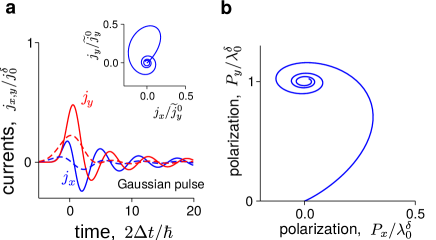
Figure S-1: ACM with Gaussian pulse a Current response for gapped Dirac systems excited by Gaussian pulse shows oscillation with $\pi/2$ phase difference between $j_{x}$ and $j_{y}$. For $j_{y}$ shown in this plot, we have used $\chi=1$. We used the Gaussian pulse widths $\delta t=\hbar/2\Delta$ (solid lines) and $\delta t=\hbar/\Delta$ (dashed lines). [Inset] Due to $\pi/2$ phase difference of $j_{x}$ and $j_{y}$, the current circulates exhibiting ACM. We used $\delta t=\hbar/2\Delta$. b Polarization (evolution over time) from the same Gaussian pulse also exhibits anomalous cyclotron motion in real space. In plotting panel b we used Gaussian pulse width $\delta t=\hbar/2\Delta$.

As a simple sanity check, we test this for a single mode drive ${\bf E}(t)={\bf E}_{0}e^{-i\omega_{0}t}$. The response should be ${\bf j}(t)=\boldsymbol{\sigma}(\omega_{0}){\bf E}_{0}e^{-i\omega_{0}t}$. Applying Eq. (S-33) we obtain

$${\bf j}(t) = \frac{1}{\pi}\int_{-\infty}^{t}dt^{\prime}{\bf E}_{0}e^{-i\omega_{0}t^{\prime}+\eta t^{\prime}}\int_{-\infty}^{\infty}d\omega{\rm Re}\,[\boldsymbol{\sigma}(\omega)]e^{-i\omega(t-t^{\prime})}$$ (S-34)

$$= \frac{{\bf E}_{0}}{\pi}\int_{-\infty}^{\infty}d\omega{\rm Re}\,[\boldsymbol{\sigma}(\omega)]\frac{-ie^{-i\omega_{0}t}}{(\omega_{0}-\omega)+i\eta}$$

$$= \frac{{\bf E}_{0}e^{-i\omega_{0}t}}{\pi}\int_{-\infty}^{\infty}d\omega{\rm Re}\,[\boldsymbol{\sigma}(\omega)]\left(\frac{-i}{(\omega_{0}-\omega)}+\pi\delta(\omega-\omega_{0})\right)$$

$$= {\bf E}_{0}e^{-i\omega_{0}t}\left(i{\rm Im}\,[\boldsymbol{\sigma}(\omega_{0})]+{\rm Re}\,[\boldsymbol{\sigma}(\omega_{0})]\right),$$

yielding the expected result. In obtaining the above, we have taken $\lim\eta\to 0$ and used the Kramers-Kronig relation to obtain ${\rm Im}\,[\boldsymbol{\sigma}]$ in the first term.

We now simulate ACM in a gapped Dirac system with a more realistic pulse: an electric field pulse with Gaussian profile $E_{x}=\frac{E_{x}^{\delta}}{\sqrt{2\pi\delta t^{2}}}\exp[-t^{2}/2\delta t^{2}]$ where $\delta t$ is the pulse width. We plug this profile into Eq. (S-33) and obtain the current response numerically in Fig. S-1. In this plot, we show current response for two cases of $\delta t=\hbar/2\Delta$ (solid lines) and $\delta t=\hbar/\Delta$ (dashed lines). We find that as long as the pulse width $\delta t$ is smaller than or about the same as $\hbar/2\Delta$, the current response is qualitatively similar to that of delta function pulse (compare Fig. S-1a in the supplement with Fig. 2a of the main text) with similar frequency oscillation; it also exhibits a similar power law decay. Increasing the pulse width obviously reduces the amplitude of oscillation (cf. solid [small pulse width] vs dashed [large pulse width] lines). Therefore, the ACM $t-$dynamics will not be seen in a single frequency continuous wave excitation. Additionally, we note that for small pulse width, the current response is insensitive to the central frequency of the Gaussian pulse. Plotting $j_{x}$ vs $j_{y}$ in the inset of Fig. S-1a shows circulating currents (ACM) due to the $\pi/2$ phase difference between $j_{x}$ and $j_{y}$. ACM turns on slowly due to finite width of the Gaussian pulse. In the long time limit; current is centered at $(0,0)$ similar to that of the delta function pulse (cf. inset of Fig.2a in the main text) since the driving field turns off at long times.

In Fig. S-1b we show the polarization of the carriers (integrated over the entire electron liquid). As expected, the charge displacement in the long time limit along $y$ reproduces that of delta function pulse (see Fig. 2b in the main text). This originates from intraband contribution to the Hall current. Along the $x$ direction, the carriers are displaced slowly at early times due to finite width of the Gaussian. At long times, the total change of polarization in $x$ vanishes since dc longitudinal conductivity is zero [see Eq. (S-25)] similar to that found for the delta function electric field pulse discussed in the main etxt.

1. ]

2. W.-K. Tse and A. H. MacDonald, Phys. Rev. Lett. 105, 057401 (2010).

3. M. Lasia and L. Brey, Phys. Rev. B 90, 075417 (2014).

4. H. Rostami and R. Asgari, Phys. Rev. B 89, 115413 (2014).

5. T. Stauber, J. Phys. Condens. Matt. 26, 123201 (2014).

References

(1)
M. I. Katsnelson, K. S. Novoselov, and A. K. Geim, Nature Physics 2, 620
( 2006).
(2)
K. S. Novoselov, A. K. Geim, S. V. Morozov, D. Jiang, Y. Zhang, S. V. Dubonos,
I. V. Grigorieva, and A. A. Firsov, Science 306(5696), 666–669 (2004).
(3)
K. S. Novoselov, A. K. Geim, S. V. Morozov, D. Jiang, M. I. Katsnelson, I. V.
Grigorieva, S. V. Dubonos, and A. A. Firsov, Nature 438, 197 (
2005).
(4)
Y. Zhang, Y.-W. Tan, H. L. Stormer, and P. Kim, Nature 438,
201– (2005).
(5)
E. N. Adams and E. I. Blount, Journal of Physics and Chemistry of Solids 10(4), 286 – 303 (1959).
(6)
R. Karplus and J. M. Luttinger, Phys. Rev. 95, 1154–1160 (1954).
(7)
G. Sundaram and Q. Niu, Phys. Rev. B 59, 14915–14925 (1999).
(8)
D. Xiao, M.-C. Chang, and Q. Niu, Rev. Mod. Phys. 82, 1959–2007
(2010).
(9)
W.-K. Tse and A. H. MacDonald, Phys. Rev. Lett. 105, 057401 (2010).
(10)
R. Nandkishore and L. Levitov, Phys. Rev. Lett. 107, 097402 (2011).
(11)
M. Lasia and L. Brey, Phys. Rev. B 90, 075417 (2014).
(12)
H. Rostami and R. Asgari, Phys. Rev. B 89, 115413 (2014).
(13)
S. P. Mukherjee and J. P. Carbotte, Phys. Rev. B 96, 085114 (2017).
(14)Supplementary Information link is provided by Publisher.
(15)
M. I. Katsnelson, Eur. Phys. J. B 51, 157-160 (2006)
Supplementary Information for “Intracell dynamics and cyclotron motion without magnetic field”
Eddwi H. Hasdeo1, Alex J. Frenzel2 and Justin C. W. Song1,3
1Institute of High Performance Computing, Agency for Science,
Technology, and Research, Singapore 138632
2Department of Physics, University of California, San Diego, La
Jolla, California, USA 92039
3Division of Physics and Applied Physics, Nanyang Technological University, Singapore 637371