11email: amueller@mpia.de 22institutetext: Univ. Grenoble Alpes, CNRS, IPAG, F-38000 Grenoble, France 33institutetext: Unidad Mixta Internacional Franco-Chilena de Astronomía, CNRS/INSU UMI 3386 and Departamento de Astronomía, Universidad de Chile, Casilla 36-D, Santiago, Chile 44institutetext: LESIA, Observatoire de Paris, Université PSL, CNRS, Sorbonne Université, Université Paris Diderot, Sorbonne Paris Cité, 5 place Jules Janssen, F-92195 Meudon, France 55institutetext: Department of Physics, University of Oxford, Oxford, UK 66institutetext: Space Telescope Science Institute, 3700 San Martin Dr. Baltimore, MD 21218, USA 77institutetext: Geneva Observatory, University of Geneva, Chemin des Mailettes 51, 1290 Versoix, Switzerland 88institutetext: INAF - Osservatorio Astronomico di Padova, Vicolo della Osservatorio 5, 35122, Padova, Italy 99institutetext: DOTA, ONERA, Université Paris Saclay, F-91123, Palaiseau France 1010institutetext: Aix Marseille Université, CNRS, LAM (Laboratoire d’Astrophysique de Marseille) UMR 7326, 13388 Marseille, France 1111institutetext: Institute for Particle Physics and Astrophysics, ETH Zurich, Wolfgang-Pauli-Strasse 27, 8093 Zurich, Switzerland 1212institutetext: Department of Astronomy, Stockholm University, AlbaNova University Center, 106 91 Stockholm, Sweden 1313institutetext: Aix Marseille Univ, CNRS, LAM, Laboratoire d’Astrophysique de Marseille, Marseille, France 1414institutetext: CRAL, UMR 5574, CNRS, Université de Lyon, Ecole Normale Supérieure de Lyon, 46 Allée d’Italie, F-69364 Lyon Cedex 07, France 1515institutetext: INAF-Osservatorio Astronomico di Brera, Via E. Bianchi 46, I-23807 Merate, Italy 1616institutetext: INCT, Universidad De Atacama, calle Copayapu 485, Copiapó, Atacama, Chile 1717institutetext: Department of Astronomy, University of Michigan, 1085 S. University Ave, Ann Arbor, MI 48109-1107, USA 1818institutetext: Leiden Observatory, Leiden University, PO Box 9513, 2300 RA Leiden, The Netherlands 1919institutetext: Physikalisches Institut, Universität Bern, Gesellschaftsstrasse 6, 3012 Bern, Switzerland 2020institutetext: Konkoly Observatory, Research Centre for Astronomy and Earth Sciences, Hungarian Academy of Sciences, P.O. Box 67,
H-1525 Budapest, Hungary 2121institutetext: Aix Marseille Univ, CNRS, LAM, Laboratoire d’Astrophysique de Marseille, UMR 7326, 13388, Marseille, France 2222institutetext: European Southern Observatory (ESO), Alonso de Còrdova 3107, Vitacura, Casilla 19001, Santiago, Chile 2323institutetext: Núcleo de Astronomía, Facultad de Ingeniería y Ciencias, Universidad Diego Portales, Av. Ejercito 441, Santiago, Chile 2424institutetext: Escuela de Ingeniería Industrial, Facultad de Ingeniería y Ciencias, Universidad Diego Portales, Av. Ejercito 441, Santiago, Chile
Orbital and atmospheric characterization of the planet within the gap of the PDS 70 transition disk††thanks: Based on observations collected at the European Organisation for Astronomical Research in the Southern Hemisphere under ESO programmes 095.C-0298, 097.C-0206, 097.C-1001, 1100.C-0481.
Abstract
Context. The observation of planets in their formation stage is a crucial, but very challenging step in understanding when, how and where planets form. PDS 70 is a young pre-main sequence star surrounded by a transition disk, in the gap of which a planetary-mass companion has been discovered recently. This discovery represents the first robust direct detection of such a young planet, possibly still at the stage of formation.
Aims. We aim to characterize the orbital and atmospheric properties of PDS 70 b, which was first identified on May 2015 in the course of the SHINE survey with SPHERE, the extreme adaptive-optics instrument at the VLT.
Methods. We obtained new deep SPHERE/IRDIS imaging and SPHERE/IFS spectroscopic observations of PDS 70 b. The astrometric baseline now covers 6 years which allows us to perform an orbital analysis. For the first time, we present spectrophotometry of the young planet which covers almost the entire near-infrared range (0.96 to 3.8 m). We use different atmospheric models covering a large parameter space in temperature, , chemical composition, and cloud properties to characterize the properties of the atmosphere of PDS 70 b.
Results. PDS 70 b is most likely orbiting the star on a circular and disk coplanar orbit at 22 au inside the gap of the disk. We find a range of models that can describe the spectrophotometric data reasonably well in the temperature range between 1000–1600 K and no larger than 3.5 dex. The planet radius covers a relatively large range between 1.4 and 3.7 with the larger radii being higher than expected from planet evolution models for the age of the planet of 5.4 Myr.
Conclusions. This study provides a comprehensive dataset on the orbital motion of PDS 70 b, indicating a circular orbit and a motion coplanar with the disk. The first detailed spectral energy distribution of PDS 70 b indicates a temperature typical for young giant planets. The detailed atmospheric analysis indicates that a circumplanetary disk may contribute to the total planet flux.
Key Words.:
Methods: observational – Techniques: spectroscopic – Astrometry – Planets and satellites: atmospheres – Planets and satellites: individual: PDS701 Introduction
Our knowledge of the formation mechanism and evolution of planets has developed by leaps and bounds since the first detection of an exoplanet by Mayor & Queloz (1995) around the main-sequence star 51 Peg. However, constraining formation time scales, the location of planet formation, and the physical properties of such objects remains a challenge and was so far mostly based on indirect arguments using measured properties of protoplanetary disks. What really is needed is a detection of planets around young stars, still surrounded by a disk. Modern coronagraphic angular differential imaging surveys such as SHINE (SpHere INfrared survey for Exoplanets, Chauvin et al. 2017), which are utilizing extreme adaptive optics, provide the necessary spatial resolution and sensitivity to find such young planetary systems.
In Keppler et al. (2018) we reported the first bona fide detection of a giant planet inside the gap of the transition disk around the star PDS 70 together with the characterization of its protoplanetary disk. PDS 70 is a K7-type 5.4 Myr young pre-main sequence member of the Upper-Centaurus-Lupus group (Riaud et al. 2006; Pecaut & Mamajek 2016) at a distance of 113.430.52 pc (Gaia Collaboration et al. 2016, 2018). Our determination of the stellar parameters are explained in detail in Appendix A. The planet was detected in five epochs with VLT/SPHERE (Beuzit et al. 2008), VLT/NaCo (Lenzen et al. 2003; Rousset et al. 2003), and Gemini/NICI (Chun et al. 2008) covering a wavelength range from to -band. In this paper we present new deep -band imaging and first spectroscopic data with SPHERE with the goal to put constraints on the orbital parameters and atmospheric properties of PDS 70 b.
2 Observations and data reduction
2.1 Observations
We observed PDS 70 during the SPHERE/SHINE GTO program on the night of February 24th, 2018. The data were taken in the IRDIFS-EXT pupil tracking mode using the N_ALC_YJH_S (185 mas in diameter) apodized-Lyot coronagraph (Martinez et al. 2009; Carbillet et al. 2011). We used the IRDIS (Dohlen et al. 2008) dual-band imaging camera (Vigan et al. 2010) with the K1K2 narrow-band filter pair ( = 2.110 0.102 m, = 2.251 0.109 m). A spectrum covering the spectral range from to -band (0.96–1.64 m, ) was acquired simultaneously with the IFS integral field spectrograph (Claudi et al. 2008). We set the integration time for both detectors to 96 s and acquired a total time on target of almost 2.5 hours. The total field rotation is 95.7°. During the course of observation the average coherence time was 7.7 ms and a Strehl ratio of 73% was measured at 1.6 m, providing excellent observing conditions.
2.2 Data reduction
The IRDIS data were reduced as described in Keppler et al. (2018). The basic reduction steps consisted of bad-pixel correction, flat fielding, sky subtraction, distortion correction (Maire et al. 2016), and frame registration.
The IFS data were reduced with the SPHERE Data Center pipeline (Delorme et al. 2017), which uses the Data Reduction and Handling software (v0.15.0, Pavlov et al. 2008) and additional IDL routines for the IFS data reduction (Mesa et al. 2015). The modeling and subtraction of the stellar speckle pattern for both the IRDIS and IFS data set was performed with an sPCA (smart Principal Component Analysis) algorithm based on Absil et al. (2013) using the same setup as described in Keppler et al. (2018).
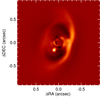
Figure 1 shows the high-quality IRDIS combined K1K2 image of PDS 70. The outer disk and the planetary companion inside the gap are clearly visible. In addition, there are several disk related features present, which are further described in Appendix B. For this image the data were processed with a classical ADI reduction technique (Marois et al. 2006) to minimize self-subtraction of the disk.
The extraction of astrometric and contrast values was performed by injecting negative point source signals into the raw data (using the unsaturated flux measurements of PDS 70) which were varied in contrast and position based on a predefined grid created from a first initial estimate of the planets contrast and position. For every parameter combination of the inserted negative planet the data were reduced with the same sPCA setup (maximum of 20 modes, protection angle of 0.75FWHM) and a value within a segment of 2FWHM and 4FWHM around the planets position was computed. Following Olofsson et al. (2016), the marginalized posterior probability distributions for each parameter was computed to derive final contrast and astrometric values and their corresponding uncertainties (the uncertainties correspond to the 68% confidence interval). For an independent confirmation of the extracted astrometry and photometry we used SpeCal (Galicher et al. 2018) and find the values in good agreement with each other within 1 uncertainty.
2.3 Conversion of the planet contrasts to physical fluxes
The measured contrasts of PDS 70 b from all data sets (SPHERE, NaCo, and NICI) were converted to physical fluxes following the approach used in Vigan et al. (2016) and Samland et al. (2017), who used a synthetic spectrum calibrated by the stellar SED to convert the measured planet contrasts at specific wavelengths to physical fluxes. In our case, instead of a synthetic spectrum which does not account for any (near-)infrared excess, we made use of the flux calibrated spectrum of PDS 70 from the SpeX spectrograph (Rayner et al. 2003) which is presented in Long et al. (2018). The spectrum covers a wavelength range from 0.7 to 2.5 , i.e. the entire IFS and IRDIS data set. To obtain flux values for our data sets taken in -band at 3.8 we modeled the stellar SED with simple black bodies to account for the observed infrared excess (Hashimoto et al. 2012; Dong et al. 2012). The final SED of the planet is shown in Fig. 2. The IFS spectrum has a steep slope and displays a few features only, mainly water absorption around . The photometric values are listed in Table 4.

3 Results
3.1 Atmospheric modeling
We performed atmospheric simulations for PDS 70 b with the self-consistent 1D radiative-convective equilibrium tool petitCODE (Mollière et al. 2015, 2017), which resulted in three different grids of self-luminous cloudy planetary model atmospheres (see Table 1).
These grids mainly differ in the treatment of clouds: petitCODE(1) does not consider scattering and includes only Mg2SiO4 cloud opacities, petitCODE(2) adds scattering, petitCODE(3) contains four more cloud species including iron (Na2S, KCl, Mg2SiO4, Fe). Additionally, we also use the publicly available cloud-free petitCODE model grid (here called petitCODE(0); see Samland et al. 2017 for a detailed description of this grid) and the public PHOENIX BT-Settl grid (Allard 2014; Baraffe et al. 2015).
In order to compare the data to the petitCODE models we use the same tools as described in Samland et al. (2017), using the python MCMC code emcee on N-dimensional model grids linearly interpolated at each evaluation. We assume a Gaussian likelihood function and take into account the spectral correlation of the IFS spectra (Greco & Brandt 2016).
For an additional independent confirmation of the results obtained using petitCODE, we also used cloudy models from the Exo-REM code. The models and corresponding simulations are described in Charnay et al. (2018). Exo-REM assumes non-equilibrium chemistry, and silicate and iron clouds. For the model grid Exo-REM(1) the cloud particles are fixed at 20 m and
the vertical distribution takes into account vertical mixing (with a parametrized ) and sedimentation.
The model Exo-REM(2) model uses a cloud distribution with a fixed sedimentation parameter as in the model by Ackerman & Marley (2001) and petitCODE.
Table 2 provides a compilation of the best-fit values and Fig. 2 shows the respective spectra. The values quoted correspond to the peak of the respective marginalized posterior probability distribution.
The cloud-free models fail to represent the data and result in unphysical parameters. In contrast, the cloudy models provide a much better representation of the data. The results obtained by the petitCODE and Exo-REM models are consistent with each other. However, because of higher cloud opacities in the Exo-REM(2) models the values are less constrained and the water feature at 1.4 m is less pronounced. Therefore, the resulting spectrum is closer to a black body and the resulting mass is less constrained. All these models indicate a relatively low temperature and surface gravity, but in some cases unrealistically high radii.
Evolutionary models predict radii smaller than 2 for planetary-mass objects (Mordasini et al. 2017).
The radius can be pushed towards lower values, if cloud opacities are removed, e.g. by removing iron (petitCODE(2)). However, a direct comparison for the same model parameters shows that this effect is very small. In petitCODE(1) this is shown in an exaggerated way by artificially removing scattering from the models, which leads to a significant reduction in radius.
In general, we find a wide range of models that are compatible with the current data. The parts of the spectrum most suitable for ruling out models are the possible water absorption feature at 1.4 m, as well as the spectral behavior at longer wavelengths ( to -band). Given the low signal-to-noise in the water absorption feature and the large uncertainties in the flux, it is very challenging to draw detailed physical conclusions about the nature of the object. We emphasize that other possible explanations for the larger than from evolutionary models expected radii, include the recent accretion of material, additional reddening by circumplanetary material, and significant flux contributions from a potential circumplanetary disk. The later possibility is especially interesting in the light of possible features in our reduced images that could present spiral arm structures close to the planet (Fig. 1). There also appears to be an increase in HCO+ velocity dispersion close to the location of the planet in the ALMA data presented by Long et al. (2018).
| Model | [M/H] | Remarks | |||||||
|---|---|---|---|---|---|---|---|---|---|
| (dex) | (dex) | ||||||||
| BT-Settl | 1200 – 3000 | 100 | 3.0 – 5.5 | 0.5 | 0.0 | – | – | – | – |
| petitCODE(0) | 500 – 1700 | 50 | 3.0 – 6.0 | 0.5 | -1.0 – 1.4 | 0.2 | – | – | cloud-free |
| petitCODE(1) | 1000 – 1500 | 100 | 2.0 – 5.0 | 1.0 | -1.0 – 1.0 | 1.0 | 1.5 | – |
w/o scattering,
w/o Fe clouds |
| petitCODE(2) | 1000 – 1500 | 100 | 2.0 – 5.0 | 0.5 | 0.0 – 1.5 | 0.5 | 0.5 – 6.0 | 1.0a𝑎aa𝑎aExcept additional grid point at 0.5 |
with scattering,
w/o Fe clouds |
| petitCODE(3) | 1000 – 2000 | 200 | 3.5 – 5.0 | 0.5 | -0.3 – 0.3 | 0.3 | 1.5 | – |
with scattering,
with Fe clouds |
| Exo-REM(1) | 400 – 2000 | 100 | 3.0 – 5.0 | 0.1 | 0.32, 1.0, 3.32 | – | – | – |
cloud particle
size fixed to m |
| Exo-REM(2) | 400 – 2000 | 100 | 3.0 – 5.0 | 0.1 | 0.32, 1.0, 3.32 | – | 1.0 | – | – |
| Model | log g | [M/H] | Radius | Massb𝑏bb𝑏bAs derived from and radius. | flux | flux | ||
|---|---|---|---|---|---|---|---|---|
| (dex) | ||||||||
| BT-Settl | 1590 | 3.5 | – | – | 1.4 | 2.4 | yes | yes |
| petitCODE(0) | 1155 | 5.5 | -1.0 | – | 2.7 | 890.0 | no | (yes) |
| petitCODE(1) | 1050 | 1.5a𝑎aa𝑎aOnly grid value. | 2.0 | 0.2 | yes | yes | ||
| petitCODE(2) | 1100 | 1.24 | 3.3 | 1.9 | yes | (no) | ||
| petitCODE(3) | 1190 | 0.0 | 2.7 | 8.9 | yes | yes | ||
| Exo-REM(1) | 1000 | 3.5 | 1.0 | – | 3.7 | 17 | yes | yes |
| Exo-REM(2) | 1100 | 4.1 | 1.0 | 1 | 3.3 | 55 | yes | yes |
3.2 Orbital properties of PDS 70 b
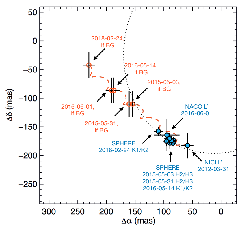
The detailed results of the relative astrometry and photometry extracted from our observation from February 2018 are listed in Table 4 together with the earlier epochs presented in Keppler et al. (2018). A first verification of the relative position of PDS 70 b with what we could expect for a stationary background contaminant is shown in Figure 3. The latest SPHERE observations of February 24th, 2018 confirms that the companion is comoving with the central star.
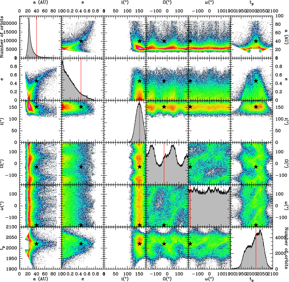
To explore the possible orbital solutions of PDS 70 b, we applied the Markov-Chain Monte-Carlo (MCMC) Bayesian analysis technique (Ford 2005, 2006) developed for Pictoris (Chauvin et al. 2012), and which is well suited for observations covering a small part of the whole orbit (for large orbital periods) as in the case of PDS 70 b. We did not initially consider any prior information on the inclination or longitude of ascending node to explore the full orbital parameter space of bound orbits. As described in Appendix A of Chauvin et al. (2012), we assume the prior distribution to be uniform in and work on a modified
parameter vector to avoid singularities in inclination and eccentricities and improve the convergence of the Markov chains. The results of the MCMC analysis are reported in Fig. 5, together with the results of a classical Least-squared linear method (LSLM) flagged by the red line. It shows the standard statistical distribution matrix of the orbital elements , , , , , and , where stands for the semi-major axis, for the eccentricity, for the inclination, the longitude of the ascending node (measured
from North), the argument of periastron and the time for periastron passage.
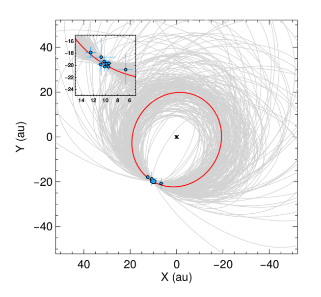
The results of our MCMC fit (Table 5) indicate orbital distributions that peak at au (the uncertainties correspond to the 68% confidence interval) for the semi-major axis, °for the inclination, eccentricities are compatible with low-eccentric solutions as shown by the (,) correlation diagram. and are poorly constrained as low-eccentric solutions are favored and as pole-on solutions are also likely possible. Time at periastron is poorly constrained. The inclination distribution clearly favors retrograde orbits (), which is compatible with the observed clockwise orbital motion resolved with SPHERE, NaCo, and NICI.
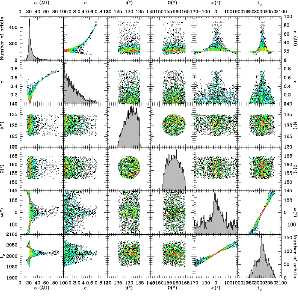
To consider the disk geometry described by Keppler et al. (2018), we decided to explore the MCMC solutions compatible with a planet-disk coplanar configuration. We restrained the PDS70 b solution set given by the MCMC to those solutions with orbital plane making a tilt angle less than 5° with respect to the disk midplane described by Keppler et al. (2018), i.e., and . The results are shown in Fig. 6 and Table 5 together with the relative astrometry of PDS 70 b reported with 200 orbital solutions randomly drawn from our MCMC distributions in Fig. 8. Figure 7 shows the posterior distribution (out of Fig. 5) of the tilt angle with the disk plane assuming and . The distribution peaks around , which remains consistent with a likely coplanar planet-disk configuration (or a moderate tilt angle) given the uncertainties. Given the small fraction of orbit covered by our observations, a broad range of orbital configurations are possible including coplanar solutions that could explain the formation of the broad disk cavity carved by PDS 70 b.
4 Summary and conclusions
We presented new deep SPHERE/IRDIS imaging data and, for the first time, SPHERE/IFS spectroscopy of the planetary mass companion orbiting inside the gap of the transition disk around PDS 70.
With the accurate distance provided by Gaia DR2 we derived new estimates for the stellar mass (0.760.02 M⊙) and age (5.41.0 Myr).
Taking into account the data sets presented in Keppler et al. (2018) we achieve an orbital coverage of 6 years. Our MCMC Bayesian analysis favors a circular au and a disk coplanar wide orbit, which translates to an orbital period of 118 yr.
The new imaging data show rich details in the structure of the circumstellar disk. Several arcs and potential spirals can be identified (see Fig. 4). How these features are connected to the presence of the planet are beyond the scope of this study.
With the new IFS spectroscopic data and photometric measurements from previous IRDIS, NaCo, and NICI observations we were able to construct a SED of the planet covering a wavelength range of 0.96 to 3.8 m. We computed three sets of cloudy model grids with the petitCODE and two models with Exo-REM with different treatment of clouds. These model grids and the BT-Settl grid were fitted to the planets’ SED. The atmospheric analysis clearly demonstrates that cloud-free models do not provide a good fit to the data. In contrast, we find a range of cloudy models that can describe the spectrophotometric data reasonably well and result in a temperature range between 1000–1600 K and no larger than 3.5 dex. The radius varies significantly between 1.4 and 3.7 RJ based on the model assumptions and is in some cases higher than what we expect from evolutionary models. The planets’ mass derived from the best fit values ranges from 2 to 17 MJ, which is similar to the masses derived from evolutionary models by Keppler et al. (2018).
This paper provides the first step into a comprehensive characterization of the orbit and atmospheric parameters of an embedded young planet. Observations with JWST and ALMA will provide additional constrains on the nature of this object, especially on the presence of a circumplanetary disk.
Acknowledgements.
SPHERE is an instrument designed and built by a consortium consisting of IPAG (Grenoble, France), MPIA (Heidelberg, Germany), LAM (Marseille, France), LESIA (Paris, France), Laboratoire Lagrange (Nice, France), INAF–Osservatorio di Padova (Italy), Observatoire de Genève (Switzerland), ETH Zurich (Switzerland), NOVA (Netherlands), ONERA (France) and ASTRON (Netherlands) in collaboration with ESO. SPHERE was funded by ESO, with additional contributions from CNRS (France), MPIA (Germany), INAF (Italy), FINES (Switzerland) and NOVA (Netherlands). SPHERE also received funding from the European Commission Sixth and Seventh Framework Programmes as part of the Optical Infrared Coordination Network for Astronomy (OPTICON) under grant number RII3-Ct-2004-001566 for FP6 (2004–2008), grant number 226604 for FP7 (2009–2012) and grant number 312430 for FP7 (2013–2016). We also acknowledge financial support from the Programme National de Planétologie (PNP) and the Programme National de Physique Stellaire (PNPS) of CNRS-INSU in France. This work has also been supported by a grant from the French Labex OSUG@2020 (Investissements d’avenir – ANR10 LABX56). The project is supported by CNRS, by the Agence Nationale de la Recherche (ANR-14-CE33-0018). It has also been carried out within the frame of the National Centre for Competence in Research PlanetS supported by the Swiss National Science Foundation (SNSF). MRM, HMS, and SD are pleased to acknowledge this financial support of the SNSF. Finally, this work has made use of the the SPHERE Data Centre, jointly operated by OSUG/IPAG (Grenoble), PYTHEAS/LAM/CESAM (Marseille), OCA/Lagrange (Nice) and Observtoire de Paris/LESIA (Paris). We thank P. Delorme and E. Lagadec (SPHERE Data Centre) for their efficient help during the data reduction process. This work has made use of the SPHERE Data Centre, jointly operated by OSUG/IPAG (Grenoble), PYTHEAS/LAM/CeSAM (Marseille), OCA/Lagrange (Nice) and Observatoire de Paris/LESIA (Paris) and supported by a grant from Labex OSUG@2020 (Investissements d’avenir – ANR10 LABX56). A.M. acknowledges the support of the DFG priority program SPP 1992 ”Exploring the Diversity of Extrasolar Planets” (MU 4172/1-1). F.Me. and M.B. acknowledge funding from ANR of France under contract number ANR-16-CE31-0013. D.M. acknowledges support from the ESO-Government of Chile Joint Comittee program ’Direct imaging and characterization of exoplanets’. J.L.B. acknowledges the support of the UK Science and Technology Facilities Council. A.Z. acknowledges support from the CONICYT + PAI/ Convocatoria nacional subvención a la instalación en la academia, convocatoria 2017 + Folio PAI77170087. We thank the anonymous referee for a constructive report on the manuscript. This work has made use of data from the European Space Agency (ESA) mission Gaia (https://www.cosmos.esa.int/gaia), processed by the Gaia Data Processing and Analysis Consortium (DPAC, https://www.cosmos.esa.int/web/gaia/dpac/consortium). Funding for the DPAC has been provided by national institutions, in particular the institutions participating in the Gaia Multilateral Agreement. This research has made use of NASA’s Astrophysics Data System Bibliographic Services of the SIMBAD database, operated at CDS, Strasbourg. Based on observations obtained at the Gemini Observatory (acquired through the Gemini Observatory Archive), which is operated by the Association of Universities for Research in Astronomy, Inc., under a cooperative agreement with the NSF on behalf of the Gemini partnership: the National Science Foundation (United States), the National Research Council (Canada), CONICYT (Chile), Ministerio de Ciencia, Tecnología e Innovación Productiva (Argentina), and Ministério da Ciência, Tecnologia e Inovação (Brazil).References
- Absil et al. (2013) Absil, O., Milli, J., Mawet, D., et al. 2013, A&A, 559, L12
- Ackerman & Marley (2001) Ackerman, A. S. & Marley, M. S. 2001, ApJ, 556, 872
- Allard (2014) Allard, F. 2014, in IAU Symposium, Vol. 299, Exploring the Formation and Evolution of Planetary Systems, ed. M. Booth, B. C. Matthews, & J. R. Graham, 271–272
- Baraffe et al. (2015) Baraffe, I., Homeier, D., Allard, F., & Chabrier, G. 2015, A&A, 577, A42
- Beuzit et al. (2008) Beuzit, J.-L., Feldt, M., Dohlen, K., et al. 2008, in Proc. SPIE, Vol. 7014, Ground-based and Airborne Instrumentation for Astronomy II, 701418
- Carbillet et al. (2011) Carbillet, M., Bendjoya, P., Abe, L., et al. 2011, Experimental Astronomy, 30, 39
- Cardelli et al. (1989) Cardelli, J. A., Clayton, G. C., & Mathis, J. S. 1989, ApJ, 345, 245
- Chabrier (2003) Chabrier, G. 2003, PASP, 115, 763
- Charnay et al. (2018) Charnay, B., Bézard, B., Baudino, J.-L., et al. 2018, ApJ, 854, 172
- Chauvin et al. (2017) Chauvin, G., Desidera, S., Lagrange, A.-M., et al. 2017, in SF2A-2017: Proceedings of the Annual meeting of the French Society of Astronomy and Astrophysics, ed. C. Reylé, P. Di Matteo, F. Herpin, E. Lagadec, A. Lançon, Z. Meliani, & F. Royer, 331–335
- Chauvin et al. (2012) Chauvin, G., Lagrange, A.-M., Beust, H., et al. 2012, A&A, 542, A41
- Choi et al. (2016) Choi, J., Dotter, A., Conroy, C., et al. 2016, ApJ, 823, 102
- Chun et al. (2008) Chun, M., Toomey, D., Wahhaj, Z., et al. 2008, in Proc. SPIE, Vol. 7015, Adaptive Optics Systems, 70151V
- Claudi et al. (2008) Claudi, R. U., Turatto, M., Gratton, R. G., et al. 2008, in Proc. SPIE, Vol. 7014, Ground-based and Airborne Instrumentation for Astronomy II, 70143E
- Cutri et al. (2003) Cutri, R. M., Skrutskie, M. F., van Dyk, S., et al. 2003, VizieR Online Data Catalog
- Delorme et al. (2017) Delorme, P., Meunier, N., Albert, D., et al. 2017, in SF2A-2017: Proceedings of the Annual meeting of the French Society of Astronomy and Astrophysics, ed. C. Reylé, P. Di Matteo, F. Herpin, E. Lagadec, A. Lançon, Z. Meliani, & F. Royer, 347–361
- Dohlen et al. (2008) Dohlen, K., Langlois, M., Saisse, M., et al. 2008, in Proc. SPIE, Vol. 7014, Ground-based and Airborne Instrumentation for Astronomy II, 70143L
- Dong et al. (2012) Dong, R., Hashimoto, J., Rafikov, R., et al. 2012, ApJ, 760, 111
- Dotter (2016) Dotter, A. 2016, ApJS, 222, 8
- Ford (2005) Ford, E. B. 2005, AJ, 129, 1706
- Ford (2006) Ford, E. B. 2006, ApJ, 642, 505
- Foreman-Mackey et al. (2013) Foreman-Mackey, D., Hogg, D. W., Lang, D., & Goodman, J. 2013, PASP, 125, 306
- Gaia Collaboration et al. (2018) Gaia Collaboration, Brown, A. G. A., Vallenari, A., et al. 2018, ArXiv e-prints [arXiv:1804.09365]
- Gaia Collaboration et al. (2016) Gaia Collaboration, Prusti, T., de Bruijne, J. H. J., et al. 2016, A&A, 595, A1
- Galicher et al. (2018) Galicher, R., Boccaletti, A., Mesa, D., et al. 2018, ArXiv e-prints [arXiv:1805.04854]
- Greco & Brandt (2016) Greco, J. P. & Brandt, T. D. 2016, ApJ, 833, 134
- Hashimoto et al. (2012) Hashimoto, J., Dong, R., Kudo, T., et al. 2012, ApJ, 758, L19
- Henden et al. (2015) Henden, A. A., Levine, S., Terrell, D., & Welch, D. L. 2015, in American Astronomical Society, AAS Meeting 225, id.336.16
- Keppler et al. (2018) Keppler, M., Benisty, M., Müller, A., et al. 2018, ArXiv e-prints [arXiv:1806.11568]
- Lenzen et al. (2003) Lenzen, R., Hartung, M., Brandner, W., et al. 2003, in Proc. SPIE, Vol. 4841, Instrument Design and Performance for Optical/Infrared Ground-based Telescopes, ed. M. Iye & A. F. M. Moorwood, 944–952
- Long et al. (2018) Long, Z. C., Akiyama, E., Sitko, M., et al. 2018, ApJ, 858, 112
- Maire et al. (2016) Maire, A.-L., Langlois, M., Dohlen, K., et al. 2016, in Proc. SPIE, Vol. 9908, Ground-based and Airborne Instrumentation for Astronomy VI, 990834
- Marois et al. (2006) Marois, C., Lafrenière, D., Doyon, R., Macintosh, B., & Nadeau, D. 2006, ApJ, 641, 556
- Martinez et al. (2009) Martinez, P., Dorrer, C., Aller Carpentier, E., et al. 2009, A&A, 495, 363
- Mayor & Queloz (1995) Mayor, M. & Queloz, D. 1995, Nature, 378, 355
- Mesa et al. (2015) Mesa, D., Gratton, R., Zurlo, A., et al. 2015, A&A, 576, A121
- Mollière et al. (2017) Mollière, P., van Boekel, R., Bouwman, J., et al. 2017, A&A, 600, A10
- Mollière et al. (2015) Mollière, P., van Boekel, R., Dullemond, C., Henning, T., & Mordasini, C. 2015, ApJ, 813, 47
- Mordasini et al. (2017) Mordasini, C., Marleau, G.-D., & Mollière, P. 2017, A&A, 608, A72
- Olofsson et al. (2016) Olofsson, J., Samland, M., Avenhaus, H., et al. 2016, A&A, 591, A108
- Pavlov et al. (2008) Pavlov, A., Möller-Nilsson, O., Feldt, M., et al. 2008, in Proc. SPIE, Vol. 7019, Advanced Software and Control for Astronomy II, 701939
- Paxton et al. (2011) Paxton, B., Bildsten, L., Dotter, A., et al. 2011, ApJS, 192, 3
- Paxton et al. (2013) Paxton, B., Cantiello, M., Arras, P., et al. 2013, ApJS, 208, 4
- Paxton et al. (2015) Paxton, B., Marchant, P., Schwab, J., et al. 2015, ApJS, 220, 15
- Pecaut & Mamajek (2016) Pecaut, M. J. & Mamajek, E. E. 2016, MNRAS, 461, 794
- Rayner et al. (2003) Rayner, J. T., Toomey, D. W., Onaka, P. M., et al. 2003, PASP, 115, 362
- Riaud et al. (2006) Riaud, P., Mawet, D., Absil, O., et al. 2006, A&A, 458, 317
- Rousset et al. (2003) Rousset, G., Lacombe, F., Puget, P., et al. 2003, in Proc. SPIE, Vol. 4839, Adaptive Optical System Technologies II, ed. P. L. Wizinowich & D. Bonaccini, 140–149
- Samland et al. (2017) Samland, M., Mollière, P., Bonnefoy, M., et al. 2017, A&A, 603, A57
- Vigan et al. (2016) Vigan, A., Bonnefoy, M., Ginski, C., et al. 2016, A&A, 587, A55
- Vigan et al. (2010) Vigan, A., Moutou, C., Langlois, M., et al. 2010, MNRAS, 407, 71
Appendix A Determination of host star properties
We use a Markov-Chain Monte-Carlo approach to find the posterior distribution for the PDS 70 host star parameters, adopting the emcee code (Foreman-Mackey et al. 2013).
The unknown parameters are the stellar mass, age, extinction, and parallax111The parallax of PDS 70 is treated as an unknown parameter in our fit to the host star’s properties, together with mass, age and . However we imposed a parallax prior, using Gaia DR2, which strongly constrains the allowed distance values. As a result, the best fit distance value reported here from the MCMC posterior draws is identical to the value provided by the Gaia collaboration., and we assume solar metallicity.
The photometric measurements used for the fit as well as the independently determined effective temperature and radius are listed in Table 3.
We perform a simultaneous fit of all these observables. The uncertainties are treated as Gaussians and we assume no covariance between them.
We use a Gaussian prior from Gaia for the distance and a Gaussian prior with mean 0.01 mag and sigma 0.07 mag, truncated at =0 mag, for the extinction (Pecaut & Mamajek 2016).
Given , we compute the extinction in all the adopted bands by assuming a Cardelli et al. (1989) extinction law.
We use a Chabrier (2003) initial mass function (IMF) prior on the mass and a uniform prior on the age.
The stellar models adopted to compute the expected observables, given the fit parameters, are from the MIST project (Paxton et al. 2011, 2013, 2015; Dotter 2016; Choi et al. 2016). These models were extensively tested against young cluster data, as well as against pre-main sequence stars in multiple system, with measured dynamical masses, and compared to other stellar evolutionary models (see Choi et al. (2016) for details).
The result of the fit constrains the age of PDS 70 to Myr and its mass to M⊙. The best fit parameter values are given by the 50% quantile (the median) and their uncertainties are based on the 16% and 84% quantile of the marginalized posterior probability distribution. The stellar parameters are identical to the values used by Keppler et al. (2018).
We note that the derived stellar age of PDS 70 is significantly younger than the median age derived for UCL with 162 Myr and an age spread of 7 Myr by Pecaut & Mamajek (2016). For the computation of the median age Pecaut & Mamajek (2016) excluded K and M-type stars for the reason of stellar activity which might bias the derived age. When the entire sample of stars is considered a median age of 91 Myr is derived. The authors provide an age of 8 Myr for PDS 70 based on evolutionary models. Furthermore, the kinematic parallax for PDS 70 therein is larger by 15% compared to the new Gaia parallax. Thus the luminosity on which the age determination is based on is underestimated and, subsequently, the age is overestimated.
| Parameter | Unit | Value | References |
|---|---|---|---|
| Distance | pc | 113.430.52 | 1 |
| K | 397236 | 2 | |
| Radius | R⊙ | 1.260.15 | computed from 2 |
| mag | 13.4940.146 | 3 | |
| mag | 12.2330.123 | 3 | |
| mag | 12.8810.136 | 3 | |
| mag | 11.6960.106 | 3 | |
| mag | 11.1290.079 | 3 | |
| mag | 9.5530.024 | 4 | |
| mag | 8.8230.040 | 4 | |
| mag | 8.5420.023 | 4 | |
| Age | Myr | 5.41.0 | this work |
| Mass | M⊙ | 0.760.02 | this work |
| mag | this work |
Appendix B The disk seen with IRDIS
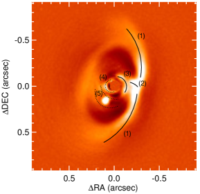
Figure 4 shows the IRDIS combined K1K2 image using classical ADI. The image shows the outer disk ring, with a radius of approximately 54 au, with the West (near) side being brighter than the East (far) side, as in Hashimoto et al. (2012) and Keppler et al. 2018. The image reveals a highly structured disk with several features: a double ring structure along the West side, which is clearly pronounced along the North-West arc, and which is less but still visible along the South-West side (1), a possible connection from the outer disk to the central region (2), a possible spiral-shaped feature close to the coronagraph (3,4), as well as two arc-like features in the gap on the South East side of the central region (5). Whereas feature (1) and (2) were already tentatively seen in previous observations (see Fig. 5 and Fig. 9 in Keppler et al. 2018), our new and unprecedentedly deep dataset allows one to identify extended structures well within the gap (features 3-5). Future observations at high resolution, i.e. with interferometry will be needed to prove the existence and to investigate the nature of these features, which, if real, would provide an excellent laboratory for probing theoretical predictions of planet-disk interactions.
Appendix C Astrometric and photometric detailed results
| Date | Instr. | Filter | (mas) | (mas) | Sep. [mas] | PA (deg) | mag | magapp | Peak SNR |
|---|---|---|---|---|---|---|---|---|---|
| 2012-03-31 | NICI | L’ | 58.710.7 | -182.722.2 | 191.921.4 | 162.23.7 | 6.590.42 | 14.500.42 | 5.6 |
| 2015-05-03 | IRDIS | H2 | 83.13.9 | -173.54.3 | 192.34.2 | 154.51.2 | 9.350.18 | 18.170.18 | 6.3 |
| 2015-05-03 | IRDIS | H3 | 83.93.6 | -178.54.0 | 197.24.0 | 154.91.1 | 9.240.17 | 18.060.17 | 8.1 |
| 2015-05-31 | IRDIS | H2 | 89.46.0 | -178.37.1 | 199.56.9 | 153.41.8 | 9.120.24 | 17.940.24 | 11.4 |
| 2015-05-31 | IRDIS | H3 | 86.96.2 | -174.06.4 | 194.56.3 | 153.51.8 | 9.130.16 | 17.950.17 | 6.8 |
| 2016-05-14 | IRDIS | K1 | 90.27.3 | -170.88.6 | 193.28.3 | 152.22.3 | 7.810.31 | 16.350.31 | 5.5 |
| 2016-05-14 | IRDIS | K2 | 95.24.8 | -175.07.7 | 199.27.1 | 151.51.6 | 7.670.24 | 16.210.24 | 3.6 |
| 2016-06-01 | NaCo | L’ | 94.522.0 | -164.427.6 | 189.626.3 | 150.67.1 | 6.840.62 | 14.750.62 | 2.7 |
| 2018-02-24 | IRDIS | K1 | 109.67.9 | -157.77.9 | 192.17.9 | 147.02.4 | 8.100.05 | 16.650.06 | 16.3 |
| 2018-02-24 | IRDIS | K2 | 110.07.9 | -157.68.0 | 192.28.0 | 146.82.4 | 7.900.05 | 16.440.05 | 13.7 |
Appendix D Markov-Chain Monte-Carlo results

| unrestrained solutions | solutions for restrained and | ||||||||
| Parameter | Unit | Peak | Median | Lower | Upper | Peak | Median | Lower | Upper |
| au | 22.2 | 25.1 | 12.5 | 28.4 | 21.2 | 23.8 | 13.3 | 27.0 | |
| 0.03 | 0.17 | 0.0 | 0.25 | 0.03 | 0.18 | 0.0 | 0.27 | ||
| ° | 151.1 | 150.1 | 137.5 | 165.2 | 131.1 | 131.0 | 128.3 | 133.6 | |
| ° | -128.1 | 0.0 | -180.0 | 51.0 | 159.6 | 158.4 | 156.2 | 163.9 | |
| ° | -130.9 | 0.0 | -180.0 | 59.9 | -12.7 | 2.5 | -144.7 | 52.3 | |
| yr | 2041.9 | 2020.1 | 2001.4 | 2069.0 | 2009.1 | 2013.4 | 1973.1 | 2029.1 | |