High Dimensional Discrete Integration over the Hypergrid

Abstract

Recently Ermon et al. (2013) pioneered a way to practically compute approximations to large scale counting or discrete integration problems by using random hashes. The hashes are used to reduce the counting problem into many separate discrete optimization problems. The optimization problems then can be solved by an NP-oracle such as commercial SAT solvers or integer linear programming (ILP) solvers. In particular, Ermon et al. showed that if the domain of integration is $\{0,1\}^{n}$ then it is possible to obtain a solution within a factor of $16$ of the optimal (a 16-approximation) by this technique.

In many crucial counting tasks, such as computation of partition function of ferromagnetic Potts model, the domain of integration is naturally $\{0,1,\dots,q-1\}^{n},q>2$, the hypergrid. The straightforward extension of Ermon et al.’s method allows a $q^{2}$-approximation for this problem. For large values of $q$, this is undesirable. In this paper, we show an improved technique to obtain an approximation factor of $4+O(1/q^{2})$ to this problem. We are able to achieve this by using an idea of optimization over multiple bins of the hash functions, that can be easily implemented by inequality constraints, or even in unconstrained way. Also the burden on the NP-oracle is not increased by our method (an ILP solver can still be used). We provide experimental simulation results to support the theoretical guarantees of our algorithms.

1 Introduction

Large scale counting problems, such as computing the permanent of a matrix or computing the partition function of a graphical probabilistic generative model, come up often in variety of inference tasks. These problems can, without loss of any generality, be written as discrete integration: the summation of evaluations of a nonnegative function $w:\Omega\to{\mathbb{R}}_{+}\cup\{0\}$ over all elements of $\Omega$:

$$S_{\Omega}(w)\equiv\sum_{\sigma\in\Omega}w(\sigma).$$ (1)

These problems are computationally intractable because of the exponential (and sometime super-exponential) size of $\Omega$. A special case is the set of problems #P, counting problems associated with the decision problems in NP. For example, one might ask how many variable assignments a given CNF (conjunctive normal form) formula satisfies. The complexity class #P was defined by Valiant [24], in the context of computing the permanent of a matrix. The permanent of a matrix $A$ is defined as,

$${\rm Perm}(A)\equiv\sum_{\sigma\in S_{n}}\prod_{i=1}^{n}A_{i,\sigma(i)},$$ (2)

where $S_{n}$ is the symmetric group of $n$ elements and $A_{i,j}$ is the $(i,j)$-th element of $A$. Clearly, here $S_{n}$ is playing the role of $\Omega$, and $w(\sigma)=\prod_{i=1}^{n}A_{i,\sigma(i)}$. Therefore computing permanent of a nonnegative matrix is a canonical example of a problem defined by eq. (1).

Similar counting problems arise when one wants to compute the partition functions of the well-known probabilistic generative models of statistical physics, such as the Ising model, or more generally the Ferromagnetic Potts Model [18]. Given a graph $G(V,E)$, and a label-space $Q\equiv\{0,1,2,\dots,q-1\}$, the partition function $Z(G)$ of the Potts model is given by,

$$\sum_{\sigma\in Q^{|V|}} \exp\Big{(}-\zeta\Big{(}J\sum_{(u,v)\in E}\delta(\sigma(u),\sigma(v))+H\sum_{u\in V}\delta(\sigma(u),0)\Big{)}\Big{)},$$ (3)

where $\zeta$, $J$ and $H$ are system-constants (representing the temperature, spin-coupling and external force), $\delta(x,y)$ is the delta-function that is $1$ if and only if $x=y$ and otherwise $0$, and $\sigma$ represents a label-vector, where $\sigma(u)$ is the label of vertex $u$.

It has been shown that, under the availability of an NP-oracle, every problem in #P can be approximated within a factor of $(1\pm\epsilon),\epsilon>0$, with high probability via a randomized algorithm [22]. This result says #P can be approximated by ${\rm BPP}^{\rm NP}$ and the power of an NP-oracle and randomization is sufficient. However, depending on the weight function $w(\cdot)$, eq. (1) may not be in #P. There are related approaches to count the number of models of propositional formulas based on SAT-solvers, such as [3, 14, 27, 17, 4, 5] among others.

The standard techniques to evaluate eq. (1) include the very influential fast variational methods [26], and Markov-Chain-Monte-Carlo based sampling schemes [12]. In practice, except for limited number of cases, these approaches are mostly used in a heuristic manner without nonasymptotic qualitative guarantees. Recently, Ermon et al. proposed an alternative approach (that they call WISH - Weighted-Integrals-And-Sums-By-Hashing) to solve these counting problems [6, 8] by breaking them into multiple optimization problems. Namely, they use families of hash functions $h:\Omega\to\tilde{\Omega},|\tilde{\Omega}|<|\Omega|,$ and use a (possibly NP) oracle that can return the correct solution of the optimization problem: $\max_{\sigma:h(\sigma)=a}w(\sigma),$ for any $a\in\tilde{\Omega}$. We call this oracle a MAX-oracle. In particular, when $\Omega=\{0,1\}^{n}$, and $h(\cdot)$ is a random hash function, assuming the availability of a MAX-oracle, Ermon et al. [6] propose a randomized algorithm that approximates the discrete sum within a factor of sixteen (a 16-approximation) with high probability. Ermon et al. use simple linear sketches over ${\mathbb{F}}_{2}$ (the finite field of size 2), i.e., the hash function $h_{A,b}:{\mathbb{F}}_{2}^{n}\to{\mathbb{F}}_{2}^{m},A\in{\mathbb{F}}_{2}^{m\times n},b\in{\mathbb{F}}_{2}^{m}$ is defined to be

$$h_{A,b}(x)=Ax+b,$$ (4)

where the arithmetic operations are over ${\mathbb{F}}_{2}$. The matrix $A$ and the vector $b$ are randomly and uniformly chosen from the respective sample spaces. The MAX-oracle in this case simply provides solutions to the optimization problem: $\max_{\sigma\in{\mathbb{F}}_{2}^{n}:A\sigma=b}w(\sigma).$

The constraint space $\{\sigma\in{\mathbb{F}}_{2}^{n}:A\sigma=b\}$ is nice since it is a coset of the nullspace of $A$, and experimental results showed them to be manageable by optimization softwares/SAT solvers. In particular it was observed that being Integer Programming constraints, real-world instances are often solved in reasonable time. Since the implementation of the hash function heavily affects the runtime, it makes sense to keep constraints of the MAX-oracle as an affine space as above. These constraints are also called parity constraints. The idea of using such constraints to show reduction among class of problems appeared in several papers before, including [20, 25, 10, 23, 11] among others. The key property that the hash functions $\{h_{A,b}\}$ satisfy is that they are pairwise independent. This property can be relaxed somewhat - and in a subsequent paper Ermon et al. show that a hash family would work even if the matrix $A$ is sparse and random, thus effectively reducing the randomness as well as making the problem more tractable empirically [7]. Subsequently, Achlioptas and Jiang [2] have shown another way of achieving similar guarantees. Instead of arriving at the set $\{\sigma\in{\mathbb{F}}_{2}^{n}:A\sigma=b\}$ as a solution of a system of linear equations (over ${\mathbb{F}}_{2}$), they view the set as the image of a lower-dimensional space. This is akin to the generator matrix view of a linear error-correcting code as opposed to the parity-check matrix view. This viewpoint allows their MAX-oracle to solve just an unconstrained optimization problem.

Drawbacks of obvious extensions of [6] to large alphabets. Note that, some crucial counting problems, such as computing the partition function of the Ferromagnetic Potts model of Eq. (3), naturally have $\Omega=\{0,1,\dots,q-1\}^{n},q>2$, i.e., a hypergrid. It is worth noting that while there exists polynomial time approximation (FPRAS) for the Ising model ($q=2$), FPRAS for general Potts model ($q>2$) is significantly more challenging (and likely impossible [9]). There are a few possible obvious extensions of Ermon et al. [6] to larger alphabets.

• (The straightforward extension). The method of [6] can be used for $q$-ary in stead of binary. However, the drawback is that it provides a $q^{2}$-approximation at best which is particularly bad if $q$ is large (or growing with $n$).

• (Convert $q$-ary to binary). To use the binary-domain algorithm of [6] for any $\Omega=\{0,1,\dots,q-1\}^{n}$, we need to use a look-up table to map $q$-ary numbers to binary. In this process the number of variables (and also the number of constraints) increases by a factor of $\log q$. This makes the MAX-oracle significantly slower, especially when $q$ is large. Also, for the permanent problem, where $|\Omega|=\exp(n\log n)$, this creates a computational bottleneck. It would be useful to extend the method of [6] for $\Omega={\mathbb{F}}_{q}^{n}$ without increasing the number of variables.

  Furthermore, when $q$ is not a power of $2$, by converting $q$-ary configurations to binary, we introduce exponentially many invalid configurations. To account for these, the MAX-oracle must be adjusted accordingly which is a difficult task. This motivates us to keep the problem in its original domain and not convert the domain to binary.

• For the binary setting, it has been noted in [6, section 5.3] that the approximation ratio can be improved to any $\alpha>1$ by increasing the number of variables, which extends to this $q$-ary setting. However this also results in an increase in number of variables by a factor of $\log_{\alpha}(q^{2})$ which is undesirable.

Our contributions. Our first contribution in this paper is to provide a new and improved algorithm to handle counting problems over nonbinary domains. For any hypergrid $\Omega=\{0,1,\dots,q-1\}^{n},q$ is a power of prime, our algorithm provides a $4(1+\frac{1}{q-1})^{2}$-approximation, when $q$ is odd, and $4(1+\frac{2}{q-2})^{2}$-approximation, when $q>2$ is even, to the optimization problem of (1) assuming availability of the MAX-oracle. Our algorithm utilizes an idea of using optimization over multiple bins of the hash function that can be easily implemented via inequality constraints. The constraint space of the MAX-oracle remains an affine space and still can be represented as a modular integer linear program (ILP). Our multi-bin technique can also be used to extend the generator-matrix based algorithm of Achlioptas and Jiang [2]. As a result, we need the MAX-oracle to only perform unconstrained maximization, as opposed to constrained. This lead to significant speed-up in the system, while resulting in the same approximation guarantees.

Finally, we show the performance of our algorithms to compute the partition function of the ferromagnetic Potts model by running experiments on both synthetic datasets and real-worlds datasets. While in this paper we concentrate on theoretical results, the experiments serve as good ‘proof of concepts’ for applications. We also use our algorithm to compute the Total Variation (TV) distance between two joint probability distributions over a large number of variables. In addition to comparing with the straightforward generalization of Ermon et al.’s method [6], we also show comparisons with the popular Markov-Chain-Monte-Carlo (MCMC) method and the belief propagation method for discrete integration. All the experiments exhibit good performance guarantees.

Organization. The paper is organized as follows. In Section 2 we describe the technique by [6] called the WISH algorithm, and then elaborate our new ideas and main results. In Section 3, we provide the main technical results that lead to an improved approximation. We provide an algorithm with unconstrained optimization oracle (similar to [2]) and its analysis in Section 4. The experimental results on computation of partition functions and total variation distance are provided in Section 5.

While only of auxiliary interest here, we note that it is possible to derandomize the hash families based on parity-constraints to the optimal extent while maintaining the essential properties necessary for their performance. Namely, it can be ensured that the hash family can still be represented as $\{x\mapsto Ax+b\}$ while using information theoretically optimal memory to generate them. We discuss this in Appendix A.

It turns out that, by using our technique and some modifications to the MAX-oracle, it is possible to obtain close-to-$4$-approximation to the problem of computing permanent of nonnegative matrices (assuming existence of NP-oracles). The NP-oracle still is amenable to be implemented in a commercial optimization solver. The idea of optimization over multiple bins is crucial here, since the straightforward generalization of Ermon et al.’s result would have given an approximation factor of $\Omega(n^{2})$. Since there exists polynomial time randomized approximation scheme ($1\pm\epsilon$-approximation) of permanent of a nonnegative matrix [13], the point of this exercise is to show that our method extends to find permanent of a matrix (albeit not with the best guarantees). We discuss this in Appendix B.

2 Background and our techniques

In this section we describe the main ideas developed by [6] and provide an overview of the techniques that we use to arrive at our new results.

Let the elements in $\Omega$ be $\sigma_{1},\sigma_{2},\dots,\sigma_{|\Omega|}$ arranged according to a decreasing order of their weight, i.e., $w(\sigma_{1})\geq w(\sigma_{2})\geq\dots\geq w(\sigma_{|\Omega|}).$ Let $\beta_{i}=w(\sigma_{q^{i}})$, for $i=0,1,\dots,n^{\prime}$, where $n^{\prime}$ is the smallest integer such that $q^{n^{\prime}}\geq|\Omega|$. When $q^{n^{\prime}}>|\Omega|$ we set $\beta_{n^{\prime}}=0$ .

Clearly $\beta_{0}\geq\beta_{1}\geq\dots\geq\beta_{n^{\prime}}$. As we have not made any assumption on the values of the weight function, $\beta_{i}$ and $\beta_{i+1}$ can be far from each other. On the other hand we can try to bound the sum $S_{\Omega}(w)$ by bounding the area of the slice between $\beta_{i}$ and $\beta_{i+1}$. This area is at least $q^{i}(\beta_{i}-\beta_{i+1})$ and at most $q^{i+1}(\beta_{i}-\beta_{i+1})$. Therefore: $\sum_{i=0}^{n^{\prime}-1}q^{i}(\beta_{i}-\beta_{i+1})+q^{n^{\prime}}\beta_{n^{\prime}}\leq S_{\Omega}(w)\leq\sum_{i=0}^{n^{\prime}-1}q^{i+1}(\beta_{i}-\beta_{i+1})+q^{n^{{}^{\prime}}}\beta_{n^{\prime}}$ which implies

$$\beta_{0}+(q-1)\sum_{i=1}^{n^{\prime}}q^{i-1}\beta_{i} \leq S_{\Omega}(w)\leq\beta_{0}+(q-1)\sum_{i=1}^{n^{\prime}}q^{i}\beta_{i}.$$ (5)

Hence $\beta_{0}+(q-1)\sum_{i=1}^{n^{\prime}}q^{i-1}\beta_{i}$ is a $q$-factor approximation of $S_{\Omega}(w)$ and if we are able to find a $k$-approximation of each value of $\beta_{i}$ we will be able to obtain a $kq$-factor approximation of $S_{\Omega}(w)$. In [6], subsequently the main idea is to estimate the coefficients $\{\beta_{i},0\leq i\leq n^{\prime}\}$.

Now note that, $q^{i}=|\{\sigma\in\Omega:w(\sigma)\geq\beta_{i}\}|,$ for $i=0,1,\dots,n^{\prime}-1$. This also hold for $i=n^{\prime}$ unless $q^{n^{\prime}}>|\Omega|$ in which case $\beta_{n^{\prime}}=0$. Suppose, using a random hash function $h:\Omega\to\{0,1,\dots,q^{i}-1\}$ we compute hashes of all elements in $\Omega$. The pre-image of an entry in $\{0,1,\dots,q^{i}-1\}$ is called the bin corresponding to that value, i.e., $\{\sigma\in\Omega:h(\sigma)=x\}$ is the bin corresponding to the value $x\in\{0,1,\dots,q^{i}-1\}$. In every bin for the hash function, there is on average one element $\sigma$ such that $w(\sigma)\geq\beta_{i}$. So for a randomly and arbitrarily chosen bin $x\in\{0,1,\dots,q^{i}-1\}$, if $w^{\ast}=\max_{\sigma:h(\sigma)=x}w(\sigma)$, then $w^{\ast}$ is a ‘good’ approximation of $\beta_{i}$ (this will be made rigorous later). Indeed, suppose one performs this random hashing $\ell=O(\log n^{\prime})$ times and then take the aggregate (in this case the median) value of $w^{\ast}$s. That is say, $\hat{w^{\ast}}={\rm median}(w^{\ast}_{1},\dots,w^{\ast}_{\ell})$. Then by using the independence of the hash functions, it can be shown that the aggregate is an upper bound on $\beta_{i}$ with high probability. In [6], $\Omega={\mathbb{F}}_{2}^{n}$ and if the hash family is pairwise independent, then by using the Chebyshev inequality it was shown that $\hat{w^{\ast}}\in[\beta_{i+2},\beta_{i-2}]$ with high probability. The WISH algorithm proposed by [6] makes use of the above analysis and provides a $2^{2\cdot 2}=16$-approximation of $S_{w}(\Omega)$. If we naively extend this algorithm for $S_{w}(\Omega)={\mathbb{F}}_{q}^{n},q>2,$ then it can be shown that $\hat{w^{\ast}}\in[\beta_{i+1},\beta_{i-1}]$ with high probability. This results in an approximation factor of $q^{2\cdot 1}=q^{2}$. For example, for a ternary alphabet, $\Omega={\mathbb{F}}_{3}^{n}$, we have a $9$-approximation to $S_{w}(\Omega).$

Instead of using a straightforward analysis for the $q$-ary case, in this paper we use a MAX-oracle that can optimize over multiple bins of the hash function. Using this oracle we proposed a modified WISH algorithm and call it MB-WISH (Multi-Bin WISH). Just as in the case of [6, 7], the MAX-oracle constraints can be integer linear programming constraints and commercial softwares such as CPLEX can be used.

The main intuition of using an optimization over multiple bins is that it boosts the probability that the $w^{\ast}$ we are getting above is close to $\beta_{i}$. To be precise, we redefined $\beta_{i}\equiv w(\sigma_{(\frac{q}{r})^{i}})$ or $(\frac{q}{r})^{i}=|\{\sigma\in\Omega:w(\sigma)\geq\beta_{i}\}|,$ for $i=1,2,\dots,n^{\prime}\equiv\lceil n\log_{q/r}q\rceil$. If we define $T(u)\equiv|\{\sigma\in\Omega:w(\sigma)\geq u\}|$, then Figure 1 illustrate the $T(u)$ vs. $u$ curve and locates $\beta_{i}$s therein. Note that, we would like to find the area under the $T(u)$ vs. $u$ curve, for which we use the sum of the vertical slices. Now to estimate the new $\beta_{i}$, we choose a hash function as before, and optimize over $r^{i}$ bins of the hash function. These steps are made rigorous in Section 3. However if we restrict ourselves to the binary alphabet then (as will be clear later) there is no immediate way to represent such multiple bins in a compact way in the MAX-oracle. For the non-binary case, it is possible to represent multiple bins of the hash function as simple inequality constraints.

This idea leads to an improvement in the approximation factor of $S_{w}(\Omega)$ to $4+\epsilon$, where $\epsilon$ decays to $0$ proportional to $q^{-1}$. Note that we need to choose $q$ to be a power of prime so that ${\mathbb{F}}_{q}$ is a field.

Figure 1: The $T(u)$ vs. $u$ curve and the illustration of $\beta_{i}$s.

In [2], the bins (as described above) are produced as images of some function, and not as pre-images of hashes. Since we want the number of bins to be $q^{i}$, this can be achieved by looking at images of $g:{\mathbb{F}}_{q}^{n-i}\to\Omega$ where $|\{g(\sigma):\sigma\in{\mathbb{F}}_{q}^{n-i}\}|=q^{n-i}.$ The rest of the analysis of [2] is almost same as above. The benefit of this approach is that the MAX-oracle just has to solve an unconstrained optimization here. Implementing our multi-bin idea for this perspective of [2] is not straight-forward as we can no longer use inequality constraints for this. However, as we show later, we found a way to combine bins here in a succinct way generalizing the design of $g$. As a result, we get the same approximation guarantee as in MB-WISH, with the oracle load heavily reduced (this algorithm, that we call Unconstrained MB-WISH, can be found in Section 4).

3 The MB-WISH algorithm and analysis

Let us assume $\Omega={\mathbb{F}}_{q}^{n}$ where $q$ is a prime-power. Let us also fix an ordering among the elements of ${\mathbb{F}}_{q}\equiv\{\alpha_{0},\alpha_{1},\dots,\alpha_{q-1}\}$ and write $\alpha_{0}\prec\alpha_{1}\prec\dots\prec\alpha_{q-1}$. In this section, the symbol ‘$\prec$’ just signifies a fixed ordering and has no real meaning over the finite field. Extending this notation, for any two vectors $x,y\in{\mathbb{F}}_{q}^{m}$, we will say $x\prec y$ if and only if the $i$th coordinates of $x$ and $y$, satisfy $x_{i}<y_{i}$ for all $i=1,\dots,m$. Below $\mathbf{1}$ denotes an all-one vector of a dimension that would be clear from context. Also, for any event ${\cal E}$ let $\mathds{1}[{\cal E}]$ denote the indicator for the event ${\cal E}$.

The MAX-oracle for MB-WISH performs the following optimization, given $A\in{\mathbb{F}}_{q}^{m\times n};b,s\in{\mathbb{F}}_{q}^{m}$:

$$\max_{\sigma\in{\mathbb{F}}_{q}^{n}:A\sigma+b\prec s}w(\sigma).$$ (6)

The modified WISH algorithm is presented as Algorithm 1. The main result of this section is below.

Algorithm 1 MB-WISH algorithm for $\Omega={\mathbb{F}}_{q}^{n}$ and a weight function $w$

0:  $r$, $\gamma=\frac{q}{3r}(\frac{1}{2}-\frac{r}{q})^{2}$, $\ell=\lceil\frac{1}{\gamma}\ln\frac{2n}{\delta}\rceil$, $n^{\prime}=\lceil n\log_{q/r}q\rceil$

  $M_{0}\equiv\max_{\sigma\in{\mathbb{F}}_{q}^{n}}w(\sigma)$

  for $i\in\{1,2,\dots,n^{\prime}\}$ do

     for $k\in\{1,\dots,\ell\}$ do

        Sample hash functions $h_{i}\equiv h_{A^{i},b^{i}}$ uniformly at random from ${\cal H}_{i,n}$ as defined in (7)

        $w_{i}^{(k)}=\max_{\sigma:A^{i}\sigma+b^{i}\prec\alpha_{r}\cdot\mathbf{1}}w(\sigma)$

     end for

     $M_{i}={\rm Median}(w_{i}^{(1)},w_{i}^{(2)},\dots,w_{i}^{(\ell)})$

  end for

  Return $M_{0}+(\frac{q}{r}-1)\sum_{i=0}^{n^{\prime}-1}M_{i+1}\big{(}\frac{q}{r}\big{)}^{i}$

Theorem 1.

Suppose $q>2$ is a prime power, $\Omega={\mathbb{F}}_{q}^{n}$ and a positive integer $r\leq\lfloor{\frac{q-1}{2}}\rfloor$. For any $\delta>0$, Algorithm 1 makes $\Theta(n\log\frac{n}{\delta})$ calls to the MAX-oracle, and with probability $\geq 1-\delta$ outputs a $(\frac{q}{r})^{2}$-approximation of $S_{w}(\Omega)$.

By setting $r=\lfloor{\frac{q-1}{2}}\rfloor$, our algorithm provides a $4(1+\frac{1}{q-1})^{2}$-approximation, when $q$ is odd, and $4(1+\frac{2}{q-2})^{2}$-approximation, when $q>2$ is even.

The constant in the big-O term in the number of calls to the oracle is a function of $q$ and $r$. In particular, when $r=\lfloor{\frac{q-1}{2}}\rfloor$ and $q$ odd, this constant varies as $q^{2}\log q$. We can tune the value of $r$ to reduce the number of calls to the oracle at the expense of the approximation factor.

The theorem will be proved by a series of lemmas. The key trick that we are using is to ask the MAX-oracle to solve an optimization problem over not a single bin, but multiple bins of the hash function. This is going to boost the probability that our estimates of $\beta_{i}$s are good. In particular we will solve the optimization over $r^{m}$ bins of the hash function. The hash family is defined in the following way. We have $h_{A,b}:{\mathbb{F}}^{n}\to{\mathbb{F}}^{m}:x\mapsto Ax+b$, the operations are over ${\mathbb{F}}_{q}$. Let

$${\cal H}_{m,n}=\{h_{A,b}:A\in{\mathbb{F}}_{q}^{m\times n},b\in{\mathbb{F}}_{q}^{m}\}.$$ (7)

For readers familiar with coding theory, the basis behind our technique is simple. The set of configurations $\{\sigma\in{\mathbb{F}}_{q}^{n}:A\sigma={\bf 0}\}$ forms a linear code of dimension $n-m$. The bins of the hash function define the cosets of this linear code. We would like to chose $q^{r}$ cosets of a random linear code and the find the optimum value of $w$ over the configurations of these cosets as the MAX-oracle. To choose a hash function uniformly and randomly from ${\cal H}$, we can just choose the entries of $A$ and $b$ uniformly at random from ${\mathbb{F}}_{q}$ independently.

Note that, the hash family ${\cal H}_{m,n}$ as defined in (7) is uniform and pairwise independent. It follows from the following more general result.

Lemma 1.

Let us define $Z_{\sigma}$ to be the indicator random variable denoting $A\sigma+b\prec\alpha_{r}\cdot\mathbf{1}$ for some $r\in\{0,\dots,q-1\}$ and $A,b$ randomly and uniformly sampled from ${\cal H}_{m,n}$. Then $\Pr(Z_{\sigma}=1)=\big{(}\frac{r}{q}\big{)}^{m}$ and for any two configurations $\sigma_{1},\sigma_{2}\in{\mathbb{F}}_{q}^{n}$ the random variables $Z_{\sigma_{1}}$ and $Z_{\sigma_{2}}$ are independent.

Proof.

Let $A_{i}$ denote the $i$th row of $i$ and $b_{i}$ denote the $i$th entry of $b$. Then $\mathds{1}[A\sigma+b\prec\alpha_{r}\cdot\mathbf{1}]=\bigwedge_{i=1}^{m}\mathds{1}[A_{i}\sigma+b_{i}\prec\alpha_{r}]$.

For all configurations $\sigma\in\Omega,\forall i$, we must have

$$\Pr(A_{i}\sigma+b_{i}\prec\alpha_{r})=\sum_{j=0}^{r-1}\Pr(A_{i}\sigma+b_{i}=\alpha_{j})=\frac{r}{q}.$$

As $A_{i},b_{i}$ are independent $1\leq i\leq m$, we must have that $\Pr(A\sigma+b\prec\alpha_{r}\cdot\mathbf{1})=(\frac{r}{q})^{m}$. Now for any two configurations $\sigma_{1},\sigma_{2}\in{\mathbb{F}}_{q}^{n}$,

$$\Pr(A_{i}\sigma_{1}+b_{i}\prec\alpha_{r}\wedge A_{i}\sigma_{2}+b_{i}\prec\alpha_{r})$$

$$=\sum_{k=0}^{r-1}\sum_{j=0}^{r-1}\Pr(A_{i}\sigma_{1}+b_{i}=\alpha_{k}\wedge A_{i}\sigma_{2}+b_{i}=\alpha_{j})$$

$$=\sum_{k=0}^{r-1}\sum_{j=0}^{r-1}\Pr(A_{i}\sigma_{1}+b_{i}=\alpha_{k})$$

$$\qquad\cdot\Pr(A_{i}\sigma_{2}+b_{i}=\alpha_{j}|A_{i}\sigma_{1}+b_{i}=\alpha_{k})$$

$$=\sum_{k=0}^{r-1}\sum_{j=0}^{r-1}\Pr(A_{i}\sigma_{1}+b_{i}=\alpha_{k})\Pr(A_{i}(\sigma_{2}-\sigma_{1})=\alpha_{j}-\alpha_{k})$$

$$=r^{2}(1/q)(1/q)=(r/q)^{2}.$$

As all the rows are independent, $\Pr(A\sigma_{1}+b\prec\alpha_{r}\cdot\mathds{1}\wedge A\sigma_{2}+b\prec\alpha_{r}\cdot\mathds{1})=(\frac{r}{q})^{2m}.$ ∎

Fix an ordering of the configurations $(\sigma_{i},1\leq i\leq q^{n})$ such that $1\leq j\leq q^{n},w(\sigma_{j})\geq w(\sigma_{j+1})$. We can also interpolate the space of configuration to make it continuous by the following technique. For any positive real number $x=z+f$, where $z=\lfloor x\rfloor$ is the integer part and $f=x-z$ is the fractional part, define $w(\sigma_{x})=w(\sigma_{z})$. For $i\in\{0,1,2,\ldots,n^{\prime}\equiv\lceil n\log_{q/r}q\rceil\}$, define $\beta_{i}=w(\sigma_{t^{i}})=w(\sigma_{\lfloor t^{i}\rfloor})$, where $t=\frac{q}{r}$. We take $w(\sigma_{k})=0$ for $k>q^{n}$. See Figure 1 for an illustration.

To prove Theorem 1 we need the following crucial lemma as well.

Lemma 2.

Let $M_{i}={\rm Median}(w_{i}^{(1)},\dots,w_{i}^{(\ell)})$ be defined as in the Algorithm 1. Then for $\gamma=\frac{q}{3r}(\frac{1}{2}-\frac{r}{q})^{2}$, we have, $\Pr\bigg{(}M_{i}\in[\beta_{\min(i+1,n^{\prime})},\beta_{\max(i-1,0)}]\bigg{)}\geq 1-2\exp(-\gamma\ell).$

Proof.

Consider the set of $\lfloor t^{j}\rfloor$ heaviest configuration

$$\Omega_{j}=\{\sigma_{1},\ldots\sigma_{\lfloor t^{j}\rfloor}\}.$$

Let $S_{j}(h_{i})=|\{\sigma\in\Omega_{j}:A^{i}\sigma+b^{i}\prec\alpha_{r}\cdot\mathbf{1}\}|.$ Recall $h_{i}$ is sampled uniformly at random from ${\cal H}_{i,n}.$ By the uniformity property of the hash function,

$${\mathbb{E}}S_{j}(h_{i})={\mathbb{E}}\sum_{\sigma\in\Omega_{j}}\mathds{1}[h_{i}(\sigma)\prec\alpha_{r}\cdot\mathbf{1}]=\frac{\lfloor t^{j}\rfloor}{t^{i}}.$$

For each configuration $\sigma$ let us denote the random variable $\bar{Z^{i}_{\sigma}}=\mathds{1}[\{h_{i}(\sigma)\prec\alpha_{r}\cdot\mathbf{1}\}]-\frac{1}{t^{i}}$. By our design ${\mathbb{E}}\bar{Z^{i}_{\sigma}}=0.$ Note that, $S_{j}(h_{i})-{\mathbb{E}}S_{j}(h_{i})=\sum_{\sigma\in\Omega_{j}}\bar{Z^{i}_{\sigma}}$. Also, from Lemma 1, the random variables $\bar{Z^{i}_{\sigma}}$s are pairwise independent. Therefore,

$$\operatorname{var}S_{j}(h_{i})=\operatorname{var}(\sum_{\sigma\in\Omega_{j}}\bar{Z^{i}_{\sigma}})=\sum_{\sigma\in\Omega_{j}}{\mathbb{E}}\bar{Z^{i}_{\sigma}}^{2}=\frac{\lfloor t^{j}\rfloor}{t^{i}}(1-\frac{1}{t^{i}}).$$

Now, for any $1\leq k\leq\ell$,

$$\Pr(w_{i}^{(k)}\geq\beta_{j})=\Pr(w_{i}^{(k)}\geq w(\sigma_{\lfloor t^{j}\rfloor}))=\Pr(S_{j}(h_{i})\geq 1)=1-\Pr(S_{j}(h_{i})\leq 0).$$

Let $j=i+1$. Then, using Chebyshev inequality,

$$\Pr(S_{j}(h_{i})\leq 0)=\Pr\Big{(}S_{j}(h_{i})-{\mathbb{E}}S_{j}(h_{i})\leq-\frac{\lfloor t^{j}\rfloor}{t^{i}}\Big{)}\leq\frac{\operatorname{var}S_{j}(h_{i})}{(\frac{\lfloor t^{j}\rfloor}{t^{i}})^{2}}\leq\frac{t^{i}(1-1/t^{i})}{\lfloor t^{j}\rfloor}<\frac{t^{i}-1}{t^{i+1}-1}\leq\frac{1}{t}=\frac{r}{q}.$$

Therefore,

$$\Pr(w_{i}^{(k)}\geq\beta_{i+1})\geq 1-\frac{r}{q}.$$

Also, $\Pr(w_{i}^{(k)}\leq\beta_{i-1})=\Pr(w_{i}^{(k)}\leq w(\sigma_{\lfloor t^{i-1}\rfloor}))\geq\Pr(S_{i-1}(h_{i})=0).$ Notice that the last inequality is satisfied because $S_{i-1}(h_{i})=0$ implies $w_{i}^{(k)}\leq w(\sigma_{\lfloor t^{i-1}\rfloor})$. Now, continuing the chain of inequalities, using Markov inequality,

$$\Pr(w_{i}^{(k)}\leq\beta_{i-1})\geq 1-\Pr(S_{i-1}(h_{i})\geq 1)\geq 1-{\mathbb{E}}S_{i-1}(h_{i})=1-\frac{\lfloor t^{i-1}\rfloor}{t^{i}}\geq 1-\frac{1}{t}=1-\frac{r}{q}.$$

Recall that, $M_{i}={\rm Median}(w_{i}^{(1)},w_{i}^{(2)},\dots,w_{i}^{(\ell)})$. Define, $X_{i}^{(k)}$ to be the indicator random variable of the event $\{w_{i}^{(k)}\leq\beta_{i+1}\}$. Therefore, $\Pr(M_{i}\leq\beta_{i+1})=\Pr(\sum_{k=1}^{\ell}X_{i}^{(k)}\geq\ell/2).$ On the other hand, note that, $\Pr(X_{i}^{(k)}=1)\leq r/q$. We know from Chernoff bound that, if $X$ is a sum of iid $\{0,1\}$ random variables then $\Pr(X\geq{\mathbb{E}}X(1+\delta))\leq\exp(-{\mathbb{E}}X\delta^{2}/3)$. Therefore,

$$\Pr(M_{i}\leq\beta_{i+1})\leq\exp\Big{(}-\frac{\ell q}{3r}\Big{(}\frac{1}{2}-\frac{r}{q}\Big{)}^{2}\Big{)}.$$

Similarly,

$$\Pr(M_{i}\geq\beta_{i-1})\leq\exp\Big{(}-\frac{\ell q}{3r}\Big{(}\frac{1}{2}-\frac{r}{q}\Big{)}^{2}\Big{)}.$$

This proves the lemma. ∎

From Lemma 2, the output of the algorithm lies in the range $[L^{\prime},U^{\prime}]$ with probability at least $1-\delta$ where $L^{\prime}=\beta_{0}+(t-1)\sum_{i=0}^{n^{\prime}-1}\beta_{\min\{i+2,n^{\prime}\}}t^{i}$ and $U^{\prime}=\beta_{0}+(t-1)\sum_{i=0}^{n^{\prime}-1}\beta_{i}t^{i}$. $L^{\prime}$ and $U^{\prime}$ are a factor of $t^{2}$ apart. Now, following an argument similar to (5), we can show $L^{\prime}\leq S_{w}(\Omega)\leq U^{\prime}.$

Therefore Algorithm 1 provides a $t^{2}$-approximation to $S_{\Omega}(w)$. Let us now give the full proof of Theorem 1.

Proof of Theorem 1.

From Lemma 2, we have, $\Pr\bigg{[}\bigcap_{i=1}^{n}M_{i}\in[\beta_{\min(i+1,n^{\prime})},\beta_{\max(i-1,0)}]\bigg{]}\geq 1-2n\exp(-\gamma\ell)=1-\delta$ for $\ell=\frac{1}{\gamma}\ln\frac{2n}{\delta}$ and by definition $M_{0}=\beta_{0}.$

The algorithm outputs $M_{0}+(t-1)\sum_{i=0}^{n^{\prime}-1}M_{i+1}t^{i}$ which lies in the range $[L^{\prime},U^{\prime}]$ with probability at least $1-\delta$ where

$$L^{\prime}=\beta_{0}+(t-1)\sum_{i=0}^{n^{\prime}-1}\beta_{\min\{i+2,n^{\prime}\}}t^{i}\quad\text{ and }\quad U^{\prime}=\beta_{0}+(t-1)\sum_{i=0}^{n^{\prime}-1}\beta_{i}t^{i}.$$

Now notice that, as $\beta_{0}\geq\beta_{1}$, we have

$$U^{\prime} =\beta_{0}+(t-1)\sum_{i=0}^{n^{\prime}-1}\beta_{i}t^{i}$$

$$=\beta_{0}+(t-1)(\beta_{0}+\beta_{1}t)+(t-1)\sum_{i=2}^{n^{\prime}-1}\beta_{i}t^{i}$$

$$\leq t^{2}\beta_{0}+t^{2}.(t-1).\sum_{i=2}^{n^{\prime}-1}\beta_{i}t^{i-2}$$

$$\leq t^{2}(\beta_{0}+(t-1)\sum_{i=0}^{n^{\prime}-1}\beta_{\min\{i+2,n^{\prime}\}}t^{i})=t^{2}L^{\prime}.$$

The only thing that remains to be proved is that $L^{\prime}\leq S_{w}(\Omega)\leq U^{\prime}.$ However that is true, by just following an argument similar to (5). Indeed,

$$\sum_{i=0}^{n^{\prime}-1}\beta_{i+1}(t^{i+1}-t^{i})\leq S_{\Omega}(w)\leq\sum_{i=0}^{n^{\prime}-1}\beta_{i}(t^{i+1}-t^{i})$$

which implies $L^{\prime}\leq S_{\Omega}(w)\leq U^{\prime}.$

Therefore Algorithm 1 provides a $t^{2}$-approximation to $S_{\Omega}(w)$. The total number of calls to the MAX-oracle is $n^{\prime}\ell+1=O(n\log(n/\delta))$. ∎

To exemplify this result, suppose $q=3$. In this case the algorithm provides a $9$-approximation. Later, in the experimental section, we have used a ferromagnetic Potts model with $q=5$. MB-WISH provides a $\frac{25}{4}=6.25$-approximation in that case. Note that, for a $5$-ary Potts model, it is only natural to use our algorithm instead of converting it to binary in conjunction with the original algorithm of Ermon et al.

Instead of pairwise independent hash families, if we employ $k$-wise independent families, it leads to a better decay probability of error. However it does not improve the approximation factor.

Unconstrained optimization oracle. We can modify and generalize the results of Achlioptas and Jiang [2] to formulate a version of MB-WISH that can use unconstrained optimizers as the MAX-oracle. The MAX-oracle for this algorithm performs an unconstrained optimization of the form: $\max_{\sigma\in B}w(A\sigma+b)$, given $A\in{\mathbb{F}}_{q}^{m\times n},b\in{\mathbb{F}}_{q}^{n}$ and a set $B\subseteq{\mathbb{F}}_{q}^{m}$.

The aim is to carefully design $B$ so that all the desirable statistical properties are satisfied. This part is quite different from the hashing-based analysis and not an immediate extension of [2]. We provide the algorithm (Unconstrained MB-WISH) and its analysis in the next section.

4 MB-WISH with unconstrained optimization oracle

In this section, we provide an algorithm that uses unconstrained optimizations for the oracle, as in the case of Achlioptas and Jiang [2]. We call this algorithm Unconstrained MB-WISH.

Let us assume $\Omega={\mathbb{F}}_{q}^{n}$ where $q$ is a prime-power. As before, let us also fix an ordering among the elements of ${\mathbb{F}}_{q}\equiv\{\alpha_{0},\alpha_{1},\dots,\alpha_{q-1}\}$ and write $\alpha_{0}\prec\alpha_{1}\prec\dots\prec\alpha_{q-1}$. Recall that, here the symbol ‘$\prec$’ just signifies a fixed ordering and has no real meaning over the finite field.

The MAX-oracle for Unconstrained MB-WISH performs an unconstrained optimization of the following form, given $A\in{\mathbb{F}}_{q}^{m\times n},b\in{\mathbb{F}}_{q}^{n}$ and a set $B\subseteq{\mathbb{F}}_{q}^{m}$:

$$\max_{\sigma\in B}w(A\sigma+b).$$ (8)

The Unconstrained MB-WISH algorithm is presented as Algorithm 2. The main result of this section is the following.

Theorem 2.

Suppose $q>2$ is a power of a prime and a positive integer $r\leq\lfloor{\frac{q-1}{2}}\rfloor$. Let $\Omega={\mathbb{F}}_{q}^{n}$. For any $\delta>0$, Algorithm 2 makes $\Theta(n\log\frac{n}{\delta})$ calls to the MAX-oracle (cf. (8)), and with probability at least $1-\delta$ outputs a $(\frac{q}{r})^{2}$-approximation of $S_{w}(\Omega)$.

Algorithm 2 Unconstrained MB-WISH algorithm for $\Omega={\mathbb{F}}_{q}^{n}$ and a weight function $w$

0:  $\ell\rightarrow\lceil\frac{1}{\gamma}\ln\frac{2n}{\delta}\rceil$, $r,n^{\prime}=\lceil n\log_{q/r}q\rceil$

  $M_{0}\equiv\max_{\sigma\in{\mathbb{F}}_{q}^{n}}w(\sigma)$

  for $i\in\{1,2,\dots,n\}$ do

     for $k\in\{1,\dots,\ell\}$ do

        Sample a full rank matrix uniformly at random from the set of all full rank $n\times n$ matrices in ${\mathbb{F}}_{q}^{n\times n}$ and construct matrices $A$ and $R$ by taking the first $n-i$ columns and the last $i$ columns respectively. Sample $b\in{\mathbb{F}}_{q}^{n}$ uniformly at random

        $w_{i}^{(k)}=\max_{\begin{subarray}{c}x\in{\mathbb{F}}_{q}^{n-i}\\ y\in\{\alpha_{0},\alpha_{1},\dots,\alpha_{r-1}\}^{i}\end{subarray}}w(Ax+Ry+b)$

     end for

     $M_{i}={\rm Median}(w_{i}^{(1)},w_{i}^{(2)},\dots,w_{i}^{(\ell)})$

  end for

  for $i\in\{n+1,\dots,n^{\prime}\}$ do

     for $k\in\{1,\dots,\ell\}$ do

        Sample full rank matrix $A\in{\mathbb{F}}_{q}^{n\times n},b\in{\mathbb{F}}_{q}^{n}$ uniformly at random. Set $\mathcal{S}_{i}$ as defined in Equation (10)

        $w_{i}^{(k)}=\max_{y\in\mathcal{S}_{i}}w(Ay+b)$

     end for

     $M_{i}={\rm Median}(w_{i}^{(1)},w_{i}^{(2)},\dots,w_{i}^{(\ell)})$

  end for

  Return $M_{0}+(\frac{q}{r}-1)\sum_{i=0}^{n^{\prime}-1}M_{i+1}\big{(}\frac{q}{r}\big{)}^{i}$

To prove this theorem we borrow some ideas from coding theory. We define a linear $q$-ary code $C$ of dimension $n-m$ and length $n$ as the set of vectors $\{Ax:x\in{\mathbb{F}}_{q}^{n-m}\}$ where $A$ is a full-rank matrix of size $n\times n-m$ and rank $n-m$. For a vector $a\in{\mathbb{F}}_{q}^{n}$, we define the set $\{a+C\}$ as a coset of $C$. It is well known that ${\mathbb{F}}_{q}^{n}$ is partitioned by the $q^{m}$ distinct cosets, each of size $q^{n-m}$. The main technique behind our algorithm is that for a random linear code $C$ of size $q^{n-m}$, we randomly sample $r^{m}$ distinct cosets of $C$. Subsequently, we find the maximum value $w(x)$ of an element among those $r^{m}$ cosets.

Let $E\in{\mathbb{F}}_{q}^{n\times n}$ be an $n\times n$ full rank matrix randomly and uniformly chosen from the set of all $n\times n$ rank-$n$ matrices over ${\mathbb{F}}_{q}$. One can choose such a matrix via rejection sampling: independently and uniformly sample the entries of the matrix from ${\mathbb{F}}_{q}$ and then reject the matrix and resample it if it is not full rank. Let $A$ denote the random matrix formed by the first $n-m$ columns of $E$ as columns and let $R$ be the random matrix formed by the remaining $m$ columns of $E$ as columns. Also let $b$ be a vector sampled randomly and uniformly from ${\mathbb{F}}_{q}^{n}$. The MAX-oracle for Unconstrained MB-WISH is going to perform the following optimization when $m\leq n$:

$$\max_{\sigma_{1}\in{\mathbb{F}}_{q}^{n-m},\sigma_{2}\in\{\alpha_{0},\alpha_{1},\dots,\alpha_{r-1}\}^{m}}w(A\sigma_{1}+R\sigma_{2}+b).$$ (9)

Analogous to Theorem 1, here we are creating union of $r^{m}$ distinct random bins. If we can prove that, for any element of ${\mathbb{F}}_{q}^{n}$, the probability that it belongs to one of these bins is $(\frac{r}{q})^{m}$ and for any pair of different elements from ${\mathbb{F}}_{q}^{n}$, whether they belong to one of these bins are independent (pairwise independence), the rest of the proof of Theorem 2 will just follow that of Theorem 1.

In particular, we just have to prove the lemma that is analogous to Lemma 1. Define a set

$$S_{A,R,b}\equiv\{Ax+b+Ry\mid x\in{\mathbb{F}}_{q}^{n-m},y\in\{\alpha_{0},\alpha_{1},\dots,\alpha_{r-1}\}^{m}\}.$$

For each configuration $\sigma\in{\mathbb{F}}_{q}^{n}$, associate an indicator random variable $Z_{\sigma}$ denoting whether $\sigma\in S_{A,R,b}$ .

Lemma 3.

For each configuration $\sigma\in{\mathbb{F}}_{q}^{n}$, we must have $\Pr(Z_{\sigma}=1)=\Big{(}\frac{r}{q}\Big{)}^{m}$ and moreover for any two distinct configurations $\sigma_{1},\sigma_{2}\in{\mathbb{F}}_{q}^{n}$, we must have $\Pr(Z_{\sigma_{1}}=1\wedge Z_{\sigma_{2}}=1)\leq(\Pr(Z_{\sigma}=1))^{2}$.

Proof.

Notice that $S_{A,R,b}$ is a union of distinct cosets and therefore,

$$S_{A,R,{\bf 0}}\equiv\bigcup_{y\in\{\alpha_{0},\alpha_{1},\dots,\alpha_{r-1}\}^{m}}S_{A,{\bf 0}}(y),$$

where $S_{A,{\bf 0}}(y)\equiv\{Ax+Ry\mid x\in{\mathbb{F}}_{q}^{n-m}\}$ is defined as a particular coset with a fixed $y\in\{\alpha_{0},\alpha_{1},\dots,\alpha_{r-1}\}^{m}$. Hence $|S_{A,R,{\bf 0}}|=q^{n-m}r^{m}$ and since $S_{A,R,b}$ is simply a random affine shift of $S_{A,R,{\bf 0}}$, $|S_{A,R,b}|=q^{n-m}r^{m}$ as well. Now for a vector $\sigma\in{\mathbb{F}}_{q}^{n}$, we must have

$$\Pr(Z_{\sigma}=1)=\sum_{y\in S_{A,R,b}}\Pr(\sigma=y)=\frac{|S_{A,R,b}|}{q^{n}}=\Big{(}\frac{r}{q}\Big{)}^{m}.$$

Next, for two configurations $\sigma_{1},\sigma_{2}\in{\mathbb{F}}_{q}^{n}$, we have that

$$\Pr(Z_{\sigma_{1}}=1\wedge Z_{\sigma_{2}}=1) =\sum_{y_{1},y_{2}}\Pr(\sigma_{1}\in S_{A,b}(y_{1})\wedge\sigma_{2}\in S_{A,b}(y_{2}))$$

$$=\sum_{y_{1},y_{2}}\Pr(\sigma_{1}\in S_{A,b}(y_{1})\mid\sigma_{2}\in S_{A,b}(y_{2}))\Pr(\sigma_{2}\in S_{A,b}(y_{2}))$$

$$=\sum_{y_{1},y_{2}}\Pr(\sigma_{1}-\sigma_{2}\in S_{A,{\bf 0}}(y_{1}-y_{2}))\Pr(\sigma_{2}\in S_{A,b}(y_{2})).$$

Therefore we just need to evaluate the probability of the event $\Pr(\tau\in S_{A,{\bf 0}}(z))$ for $\tau=\sigma_{1}-\sigma_{2}\neq 0$ and $z=y_{1}-y_{2}$. Now, if $z={\bf 0}$, $\Pr(\tau\in S_{A,{\bf 0}}(\bf{0}))$ is equal to $\frac{q^{n-m}-1}{q^{n}-1}$ since $A$ is a randomly chosen full rank matrix, i.e., $|\{Ax:x\in{\mathbb{F}}_{q}^{n-m}\}|\setminus\{0\}=q^{n-m}-1$. Now, since $\{Ax+Rz:x\in{\mathbb{F}}_{q}^{n-m}\},z\neq 0,$ is a uniformly random coset of $\{Ax:x\in{\mathbb{F}}_{q}^{n-m}\}$, we have,

$$\Pr(\tau\in S_{A,{\bf 0}}(z)\mid z\neq 0,\tau\in\{Ax:x\in{\mathbb{F}}_{q}^{n-m}\})=0$$

and $$\Pr(\tau\in S_{A,{\bf 0}}(z)\mid z\neq 0,\tau\notin\{Ax:x\in{\mathbb{F}}_{q}^{n-m}\})=\frac{1}{q^{m}-1}.$$

Hence,

$$\Pr(\tau\in S_{A,{\bf 0}}(z)\mid z\neq 0) =\Big{(}1-\frac{q^{n-m}-1}{q^{n}-1}\Big{)}\frac{1}{q^{m}-1}=\frac{q^{n-m}}{q^{n}-1}.$$

Therefore, we have that

$$\Pr(Z_{\sigma_{1}}=1\wedge Z_{\sigma_{2}}=1) =\sum_{y_{1},y_{2}:y_{1}=y_{2}}\frac{q^{n-m}-1}{q^{n}-1}+\sum_{y_{1},y_{2}:y_{1}\neq y_{2}}\frac{q^{n-m}}{q^{n}-1}$$

$$=r^{m}\Big{(}\frac{q^{n-m}-1}{q^{n}-1}\Big{)}+\Big{(}r^{2m}-r^{m}\Big{)}\Big{(}\frac{q^{n-m}}{q^{n}-1}\Big{)}$$

$$=\frac{r^{m}(r^{m}q^{n-m}-1)}{q^{n}-1}$$

$$\leq\Big{(}\frac{r}{q}\Big{)}^{2m}=\Pr(Z_{\sigma_{1}}=1)^{2}$$

and hence we have the statement of the lemma. ∎

Although the two random variables $Z_{\sigma_{1}}$ and $Z_{\sigma_{2}}$ defined above are not independent, we show that they are negatively correlated. Note that, the pairwise independence was then subsequently used in computing a variance for the Chebyshev’s inequality (see Lemma 2). However, the negative correlation is sufficient to obtain an upper bound on the variance.

From Algorithm 2 it is clear that Lemma 3 allows us to obtain the values of $M_{i}$ for $i\in\{1,2,\dots,n\}$. Indeed, the MAX-oracle is not well defined when $m>n$. In order to obtain the values of $M_{i}$ for $i\in\{n+1,\dots,n^{\prime}\}$, we propose the following technique.

Recall that the elements of ${\mathbb{F}}_{q}^{n}$ can be represented as $n$ dimensional vectors where each element belongs to ${\mathbb{F}}_{q}$. Moreover we defined an ordering over the elements of the finite field ${\mathbb{F}}_{q}\equiv\{\alpha_{0},\alpha_{1},\dots,\alpha_{q-1}\}$ so that $\alpha_{i}\prec\alpha_{j}$ for $i<j$. Consider the lexicographic ordering of the elements (vectors) of ${\mathbb{F}}_{q}^{n}$. Let $s_{m}$ be the $\lceil\frac{r^{m}}{q^{m-n}}\rceil$ th element in this ordering of ${\mathbb{F}}_{q}^{n}$. Define the set

$$\mathcal{S}_{m}=\{x\in{\mathbb{F}}_{q}^{n}\mid x\prec s_{m}\}$$ (10)

for all $m>n$. Now, let $A\in{\mathbb{F}}_{q}^{n\times n}$ be an $n\times n$ full rank matrix randomly and uniformly chosen from the set of all $n\times n$ rank-$n$ matrices over ${\mathbb{F}}_{q}$, which can be generated by rejection sampling as before. Let $b\in{\mathbb{F}}_{q}^{n}$ be a uniform random vector. Subsequently, the MAX-Oracle for Unconstrained MB-WISH solves the following optimization problem for $m>n$:

$$\max_{y\in\mathcal{S}_{m}}w(Ay+b).$$

In order to analyze the statistical properties of this oracle, define the random set

$$T_{A,b,m}\equiv\{Ay+b\mid y\in\mathcal{S}_{m}\}.$$

Again, for each configuration $\sigma\in{\mathbb{F}}_{q}^{n}$, associate an indicator random variable $Z_{\sigma}$ denoting $\sigma\in T_{A,b,m}$.

Lemma 4.

For each configuration $\sigma\in{\mathbb{F}}_{q}^{n}$, we must have $\Big{(}\frac{r}{q}\Big{)}^{m}-\frac{1}{q^{n}}\leq\Pr(Z_{\sigma}=1)\leq\Big{(}\frac{r}{q}\Big{)}^{m}$ and moreover for any two configurations $\sigma_{1},\sigma_{2}\in{\mathbb{F}}_{q}^{n}$, $\Pr(Z_{\sigma_{1}}=1\wedge Z_{\sigma_{2}}=1)\leq(\Pr(Z_{\sigma}=1))^{2}.$

Proof.

We have,

$$\Pr(Z_{\sigma}=1)=\sum_{y\in T_{A,b,m}}\Pr(\sigma=y)=\frac{|T_{A,b,m}|}{q^{n}}=\frac{1}{q^{n}}\Big{\lfloor}\frac{r^{m}}{q^{m-n}}\Big{\rfloor},$$

which proves the first claim. Next, for two distinct configurations $\sigma_{1},\sigma_{2}\in{\mathbb{F}}_{q}^{n}$, we have that

$$\Pr(Z_{\sigma_{1}}=1\wedge Z_{\sigma_{2}}=1) =\sum_{y_{1},y_{2}\in T_{A,b,m}}\Pr(\sigma_{1}=y_{1}\wedge\sigma_{2}=y_{2})$$

$$=\sum_{y_{1},y_{2}\in\mathcal{S}_{m}}\Pr(\sigma_{1}=Ay_{1}+b\wedge\sigma_{2}=Ay_{2}+b)$$

$$=\sum_{y_{2}\in\mathcal{S}_{m}}\Pr(\sigma_{2}=Ay_{2}+b)\sum_{y_{1}\in\mathcal{S}_{m}}\Pr(\sigma_{1}=Ay_{1}+b\mid\sigma_{2}=Ay_{2}+b)$$

$$=\sum_{y_{2}\in\mathcal{S}_{m}}\Pr(\sigma_{2}=Ay_{2}+b)\sum_{y_{1}\in\mathcal{S}_{m}}\Pr(\sigma_{1}-\sigma_{2}=A(y_{1}-y_{2}))$$

Since $\sigma_{1}\neq\sigma_{2}$, we must have that $\Pr(\sigma_{1}-\sigma_{2}=A(y_{1}-y_{2})\mid y_{1}=y_{2})=0$. For $y_{1}\neq y_{2}$, every configuration $\sigma\in{\mathbb{F}}_{q}^{n},\sigma\neq 0$ is equally probable to be $A(y_{1}-y_{2})$ since $A$ is uniformly and randomly sampled full rank matrix. Hence,

$$\Pr(Z_{\sigma_{1}}=1\wedge Z_{\sigma_{2}}=1) =\frac{1}{q^{n}(q^{n}-1)}\Big{\lfloor}\frac{r^{m}}{q^{m-n}}\Big{\rfloor}\Big{(}\Big{\lfloor}\frac{r^{m}}{q^{m-n}}\Big{\rfloor}-1\Big{)}\leq(\Pr(Z_{\sigma}=1))^{2}.$$

∎

The remainder of the proof of Theorem 2 follows that of Theorem 1 in a straightforward manner.

5 Experimental results

All the experiments were performed in a shared parallel computing environment that is equipped with 50 compute nodes with 28 cores Xeon E5-2680 v4 2.40GHz processors with 128GB RAM.

Experiments on simulated Potts model (regular degree graph).

We implemented our algorithm to estimate the partition function of Potts Model. Recall that the partition function of the Potts model on a graph $G=(V,E)$ is given in Eq. (3). First of all, we computed partition functions for small graphs where a brute-force algorithm can also be used. For our simulation, we have randomly generated the graph $G$ with number of nodes $n\equiv|V|$ varying in $4,5,6,7,8,9,$ and corresponding regular degree $d=2,2,4,4,4,4,$ using a python library networkx. We took the number of states of the Potts model $q=5$, the external force $H$ and the spin-coupling $J$ to be 0.1 and then varied the values of $\zeta$. The partition functions for different cases are calculated using both brute force and our algorithm (MB-WISH). We have used a python module constraint to handle the constrained optimization for MAX-oracle. The obtained approximation factors for different $\zeta$ are listed in Table 1. The worst approximation factor observed in all these trials is $5.442$. This experiment shows that, for small graphs the partition functions computed by MB-WISH are good approximations to the actual values.

$\zeta$	$n=4,d=2$	$n=5,d=2$	$n=6,d=4$	$n=7,d=4$	$n=8,d=4$	$n=9,d=4$
0	0.976	1.220	0.610	1.907	0.953	1.192
5	0.580	0.708	1.639	0.755	0.630	0.599
10	0.7470	1.191	3.271	0.989	1.875	1.25
15	1.430	1.036	1.013	1.224	1.399	1.692
20	1.032	1.590	1.141	1.173	1.365	1.491
25	0.839	1.118	1.339	1.035	1.429	1.326
30	0.510	4.0562	2.226	1.060	0.690	2.122
35	1.073	5.442	0.489	2.871	1.639	1.263
40	1.210	2.434	0.980	0.582	0.666	0.969
45	1.127	4.640	2.348	1.336	0.3673	1.341
50	1.152	1.025	2.511	3.4307	1.1522	2.636

Table 1: The ratio of the partition function calculated by MB-WISH ($r=2$) and the actual value calculated by brute force: $\frac{\hat{Z}}{Z}$.

$n$	$\zeta=1$			$\zeta=2$			$\zeta=5$
	MB-WISH	BP	MCMC	MB-WISH	BP	MCMC	MB-WISH	BP	MCMC
10	15.16	15.51	12.60	14.35	14.98	12.06	13.07	13.56	10.65
15	23.10	23.27	20.51	22.35	22.47	19.70	19.95	20.35	17.59
20	31.04	31.03	28.69	29.98	29.96	27.62	26.93	27.13	24.80
25	38.28	38.79	36.63	37.41	37.45	35.29	33.41	33.92	31.76
30	46.23	46.55	44.49	44.51	44.94	42.89	40.82	40.705	38.65
40	61.88	62.06	59.75	59.55	59.92	57.61	54.96	54.27	51.96
50	77.31	77.58	75.28	74.69	74.90	72.59	68.62	67.84	65.54

Table 2: Log-partition function computed by unconstrained MB-WISH, Belief Propagation (BP) and Markov Chain Monte Carlo (MCMC) respectively for the cases of $\zeta=1,2$ and $5$.

For graphs with larger number of vertices, it is not possible to compute the partition function of Potts Model by brute force. Therefore, we compare the partition function computed by Unconstrained MB-WISH ($\hat{Z}$) with two standard techniques: Belief propagation (BP) [15] and Markov-Chain-Monte-Carlo (MCMC) [12]. It is known that BP provides exact result when the underlying graph is cycle-free [15]. To implement this we use the PGMPY library in python [1]. For MCMC, we employ the popular Metropolis-Hastings (MH) algorithm [16] to sample random points from $\Omega$, where we evaluate the function $w:\Omega\to{\mathbb{R}}$ and take a scaled-sum to estimate the discrete integration problem. We have calculated the average of the partition function over 10 different trials of the MH algorithm, and each trial was given the same time as that of Unconstrained MB-WISH.

Again, for our simulation, we have randomly generated the graph $G$ with number of nodes $n\equiv|V|$ varying in $10,\dots,50,$ and with regular degree $d=4$ using a python library networkx. We took the number of states of the Potts model $q=5$, the external force $H$ and the spin-coupling to be $0.1$ and then varied the values of $\zeta$. In our experiments each optimization instances are run with a timeout of $10,15,20,20,25$ minutes for $n=20,25,30,40,50$ respectively (we let the $n=10$ case run without a time constraint). The results are summarized in Table 2. It can be observed that the partition functions computed with MCMC deviate somewhat from that computed with belief propagation, whereas MB-WISH gives values closer to the belief propagation results.

Since for cycle-free graphs, BP can provide exact result, it gives an opportunity to compare MB-WISH with the single-bin version (i.e., Ermon et al.’s original algorithm) for moderate values of $n$ and $q$. We perform the next experiment on a path-graph, which is an undirected graph where there are exactly two nodes of degree $1$ and every other node has degree $2$. We perform the experiment with the number of nodes $n\equiv|V|$ varying in $20,\dots,50$ on a path-graph such that the number of states $q=31$ and the external parameters $J=0.1$, $H=0.5$ and $\zeta=-5$. For two different values of $r$, respectively $1$ (single-bin) and $15$ (multi-bin) we compute the estimates of the partition function. We have plotted the ratio of the estimates with the corresponding ones computed by BP (which is exact), in Figure 2. It is clear from the figure and the table that the Unconstrained MB-WISH performs much better than its single-bin counterpart. The timeout for each call to the oracle is chosen to be $n/10$ where $n$ is the number of nodes in the graph.

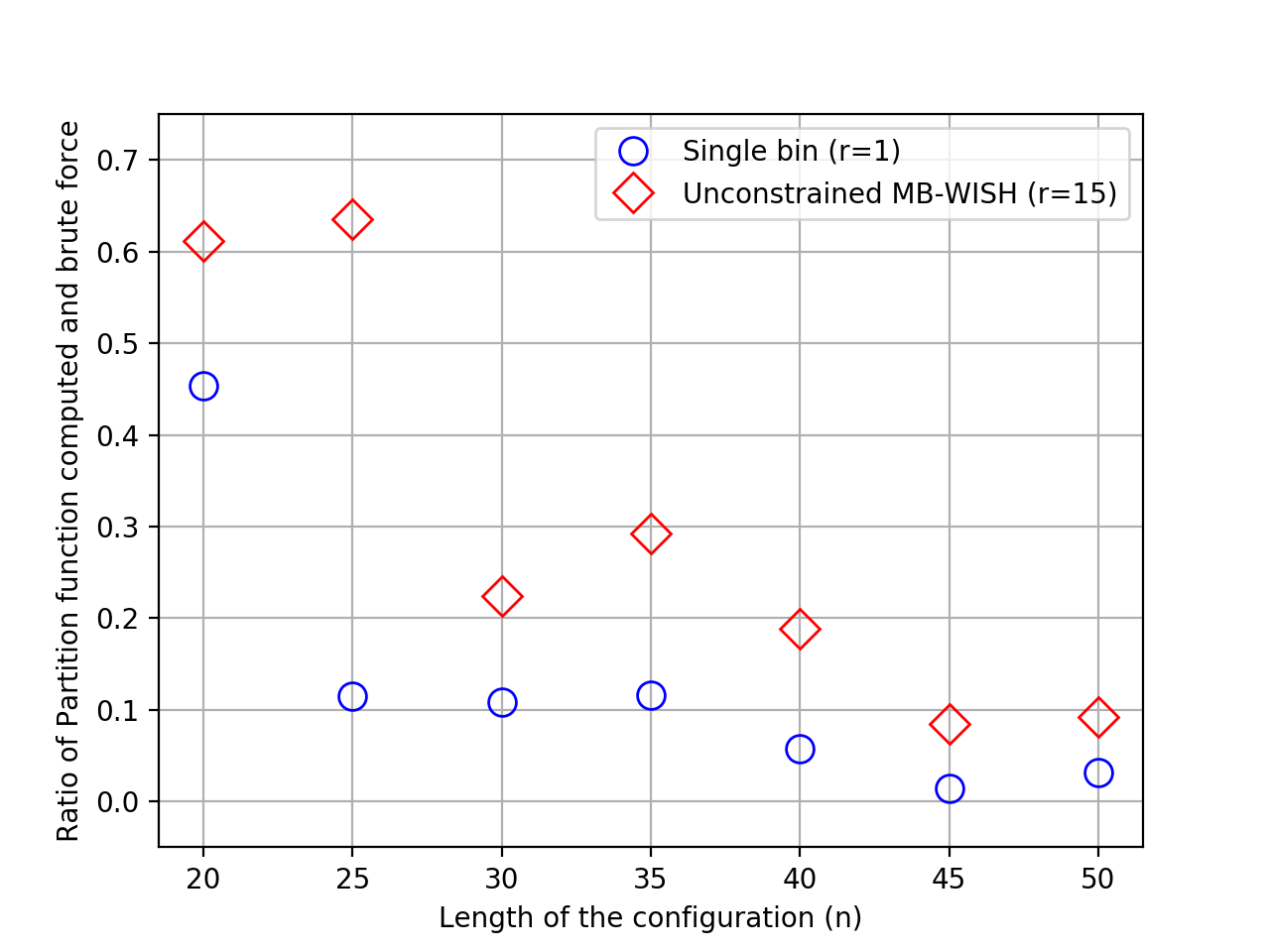
Figure 2: Comparison of approximation ratios obtained by using Unconstrained MB-WISH (red) and single-bin (Ermon et al.’s method) (blue). A ratio closer to 1 is better.

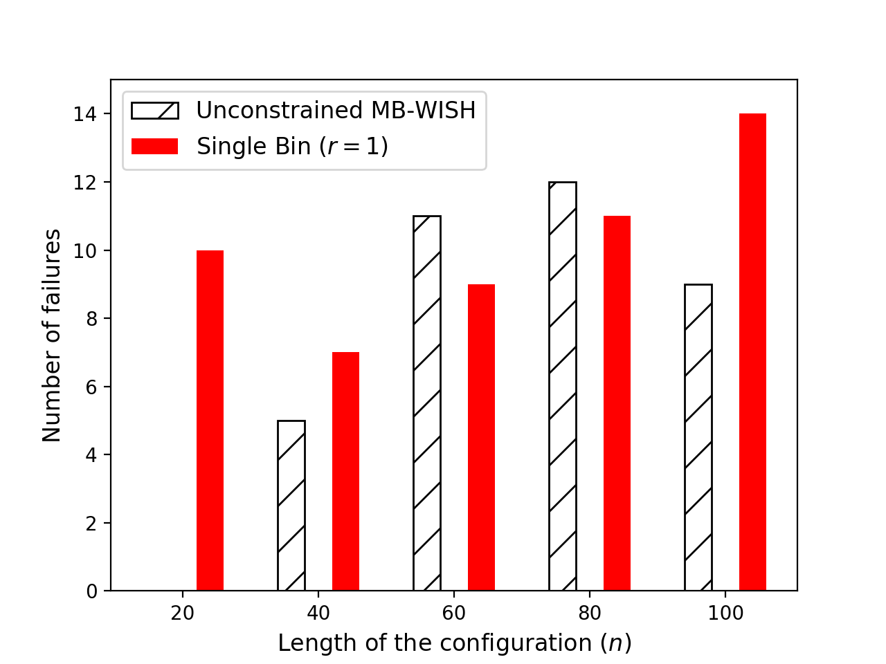
(a) Number of times, among 100 trials, the computed total variation distance is above $4\times$ the theoretical upper bound for $\epsilon=10^{-2}$

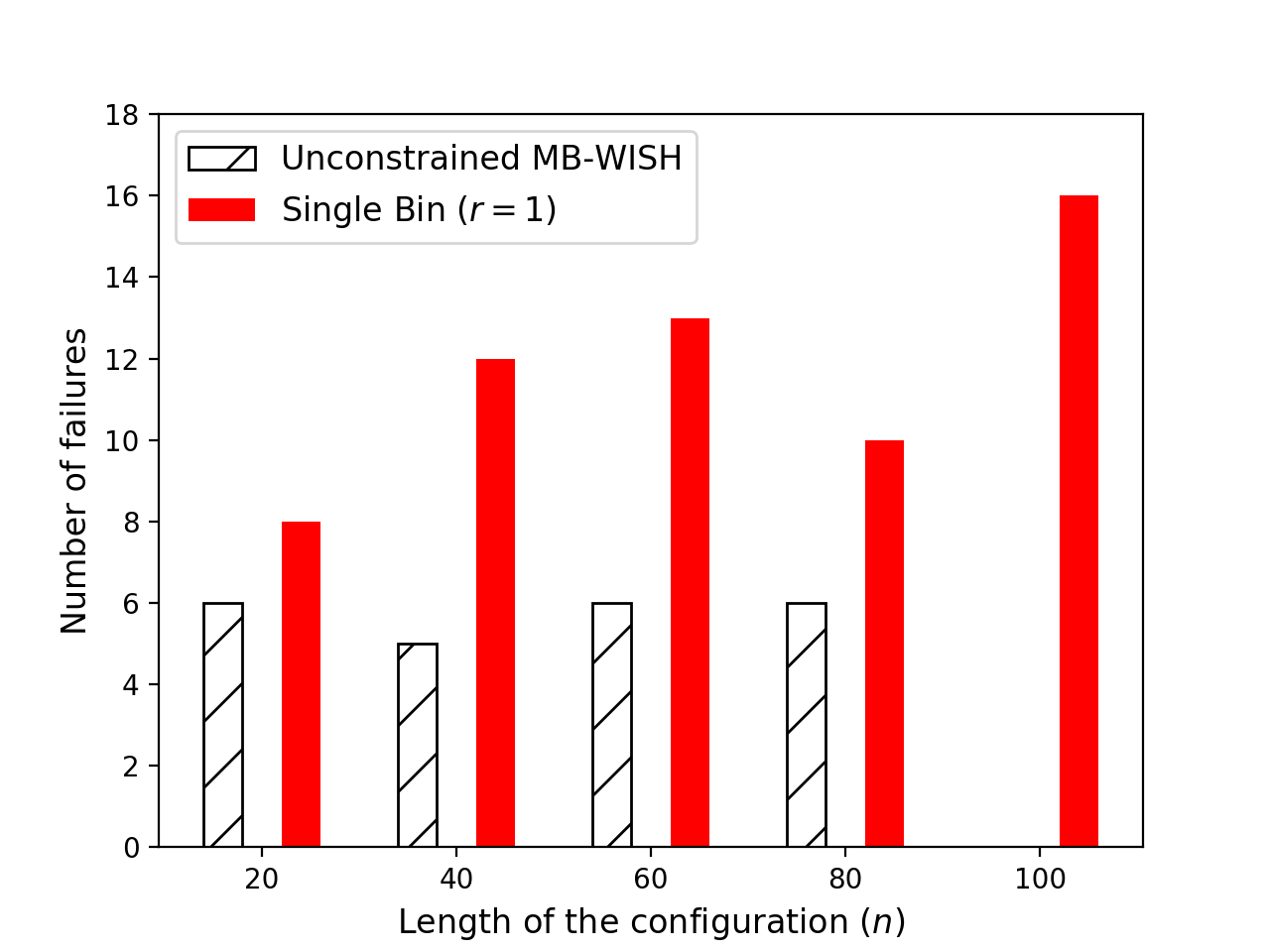
(b) Number of times, among 100 trials, the computed total variation distance is above $4\times$ the theoretical upper bound for $\epsilon=10^{-4}$

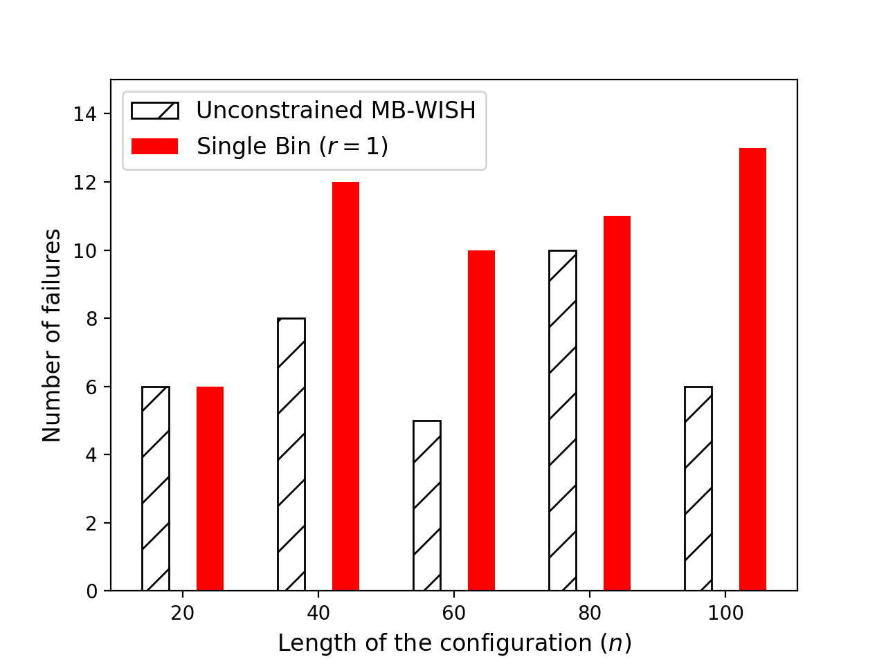
(c) Number of times, among 100 trials, the computed total variation distance is above $4\times$ the theoretical upper bound for $\epsilon=10^{-6}$

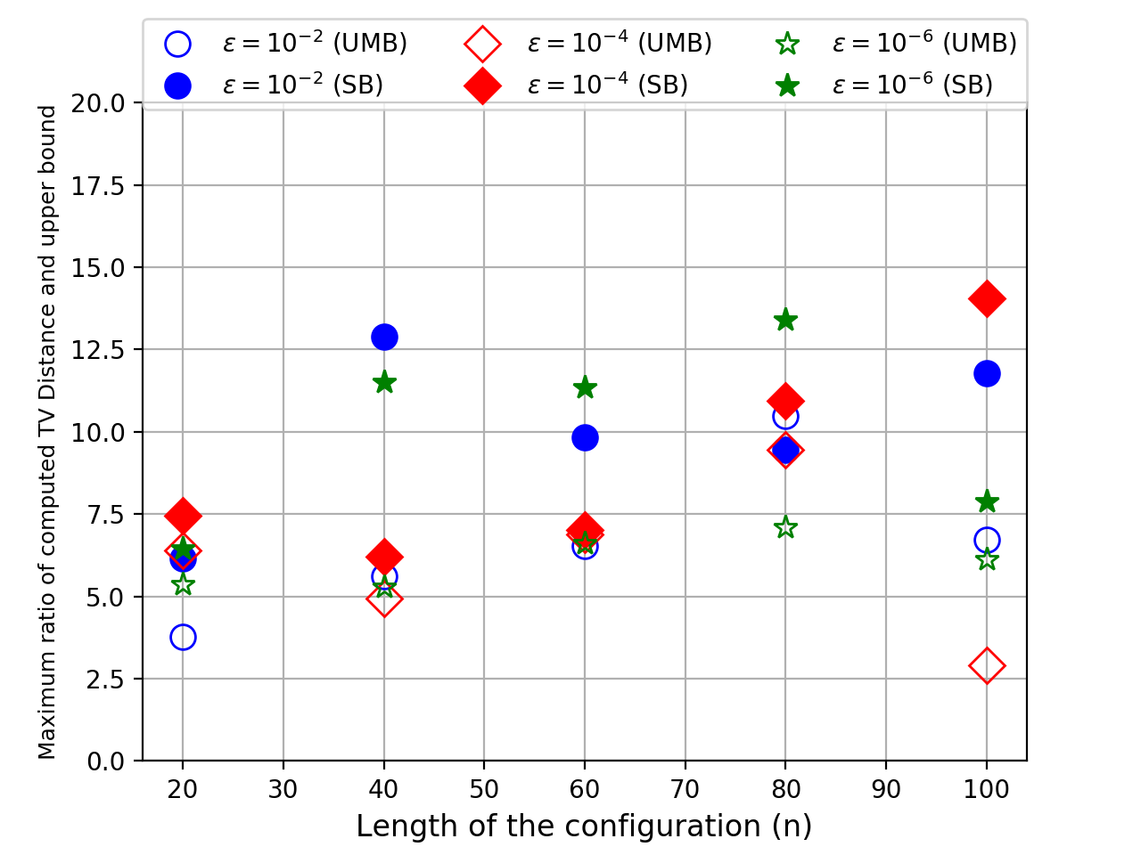
(d) The maximum ratio of the computed total variation distance and the upper bound

Figure 3: Behavior of computed total variation distance by Algorithm 2 using $r=2$ (Unconstrained MB-WISH or UMB) and $r=1$ (Single Bin or SB) with respect to the theoretical upper bound.

Experimental results on computing Total Variation distance.

We show one more instance of discrete integration where MB-WISH is useful. The purpose of this experiment is to show the effectiveness of MB-WISH by choosing counting problems where good theoretical results are available.

For this, we use Unconstrained MB-WISH to compute total variation distances between two high dimensional (up to dimension $100$) probability distributions, generated via an iid model. Although, it is computationally hard to compute the total variation distance between two distributions, for the special case of product distributions, we can derive theoretical expressions that are known to bound the total variation distance from above and below.

The total variation (TV) distance between any two discrete distributions $P$ and $Q$ with common sample space ${\cal P}$ is defined to be

$$\|P-Q\|_{TV}=\sup_{A\subseteq{\cal P}}|P(A)-Q(A)|=\frac{1}{2}\sum_{\sigma\in{\cal P}}|P(\sigma)-Q(\sigma)|.$$

Simply consider finding TV distance between joint distributions of $n$ random variables that can take value in $\{0,1,\dots,q-1\}$. In that case, we seek to find,

$$\frac{1}{2}\sum_{\sigma\in\{0,1,\dots,q-1\}^{n}}|P^{n}(\sigma)-Q^{n}(\sigma)|,$$

which is in the exact form of Eq. (1). Therefore we can use MB-WISH algorithm to estimate the total variation distance. The following are well-known upper and lower bounds on TV distance based on Hellinger distance, $h(P,Q)^{2}\equiv\sum_{\sigma\in{\cal P}}(\sqrt{P(\sigma)}-\sqrt{Q(\sigma)})^{2}$:

$$\frac{1}{2}h(P,Q)^{2}\leq\|P-Q\|_{TV}\leq h(P,Q)\sqrt{1-h(P,Q)^{2}/4}.$$

Furthermore,

$$h(P^{n},Q^{n})^{2} =2-2\prod_{i=1}^{n}(1-\frac{1}{2}h(P_{i},Q_{i})^{2}).$$

For ‘near-uniform’ distributions, it is known that the upper bound is a good approximation [19].

For the experiments, we choose two distributions defined over $q$ points in the following manner: We choose a vector $\mathbf{v}\in[0,1]^{q}$ randomly and normalize the vector (so that the sum of the elements is $1$) in order to have the first distribution $P\equiv[p_{1},p_{2},\dots,p_{q}]$. The second distribution $Q$ is then chosen to be

$$Q\equiv[p_{1},p_{2}+\epsilon,p_{3}-\epsilon,\dots,p_{q}-\epsilon].$$

where $\epsilon$ is a small number chosen in order to make the two distributions very close to each other. Here the distribution $P^{n}$ and $Q^{n}$ are supported on $\{0,1,2,\dots,q-1\}^{n}$ where $n$ can be any natural number. Now, we choose $q=5$ and for three different values of $\epsilon=10^{-2},10^{-4}$ and $10^{-6}$ and five different values of $n=20,40,60,80$ and $100$, we repeat the experiment described above $100$ times for each setting and use Unconstrained MB-WISH to compute the total variation distance.

We perform our experiments in a time constrained manner (10 minute for each calls to MAX-oracle). We have shown in Figure 3 histograms of the number of times the computed total variation distance is above four times the upper bound for $\epsilon=10^{-2},10^{-4}$ and $10^{-6}$ respectively in Figures 3(a), 3(b) and 3(c) respectively. We chose a factor of four because the theoretical approximation factor guaranteed by Unconstrained MB-WISH is $\sim 4$. We observed that the total variation distance is always above the upper bound with Hellinger distance but on the other hand, in very few trials the computed value is above four times the upper bound. Finally, we have also shown the maximum ratio of the computed total variation distance and the upper bound for each value of $\epsilon$ and $n$ in Figure 3(d).

We have compared the results obtained by Unconstrained MB-WISH with the corresponding results obtained by its single bin counterpart (Ermon et al.’s method, choosing $r=1$) in Figure 3. Even though $q=5$ is not large, the improvement in performance by using Unconstrained MB-WISH is clear. In Figures 3(a), 3(b), 3(c), it can be observed that in the case of single bin, the number of failures (solid red) is almost always larger than the corresponding setting with multiple bins. Moreover, in Figure 3(d), the maximum ratio in the setting of single bin (solid) is always much higher than the the setting of multiple bins (hollow).

Real-world constraint satisfaction problem (CSPs).

Many instances of real-world graphical models are available in http://www.cs.huji.ac.il/project/PASCAL/showExample.php. Notably, some of them (e.g., image alignment, protein folding) are defined on non-Boolean domains, which justify the use of MB-WISH. We have computed the partition functions for several of them.

The dataset Network.uai is a Markov network with $120$ nodes each having a binary value. A configuration here is a binary sequence of length $120$. To calculate the partition function, we need to find the sum of weights for $2^{120}$ different configurations. In order to use Unconstrained MB-WISH, we view each configuration as a $16$-ary string of length $30$. Our results for the log-partition came out to be $156.00$ with one hour time out for each call to the MAX-oracle. The benchmark for the log-partition function is provided to be $163.204$.

The Object detection dataset comprised of $60$ nodes each having a $11$-ary value and by Unconstrained MB-WISH we found the log-partition function to be $-38.9334$. The CSP dataset is a Markov network with $30$ node having a ternary value: we found the log partition function to be $-39.9933$. For these datasets there were no baselines available for comparison. The purpose of these experiments were to establish the scalability of MB-WISH.

6 Conclusion

Large scale counting problems (or discrete integrations of nonnegative weight functions) are often computationally intractable, but come up frequently in variety of inference tasks, most prominently as evaluations of partition functions. In this paper we extend a recent technique of hashing and optimization due to Ermon et al. for discrete integration over hypercube $\{0,1\}^{n}$ to that over hypergrids $\{0,1,\dots,q-1\}^{n}$. The trivial generalization results in an approximation factor that rapidly becomes worse as $q$ increases. We remedy the situation by providing constant factor approximation algorithms for all $q.$

The main drawback of this approach of discrete integration is the delegation of a hard combinatorial optimization to an oracle. In this line of work, an open problem is to come up with hash functions that maintain the essential properties (such as pairwise independence), but make the oracle optimization amenable. While in general this is not possible, for certain classes of weight functions this may be a plausible task and requires further exploration.

Appendix A Derandomization: structured hashes

For the analysis of [6, 7] to go through, we needed a family of hash functions that are pairwise independent. A hash family ${\cal H}=\{h:\Omega\to\tilde{\Omega}\}$ is called uniform and pairwise independent if the following two criteria are met for a randomly and uniformly chosen $h$ from ${\cal H}$: 1) for every $x\in\Omega,$ $h(x)$ is uniformly distributed in $\tilde{\Omega}$ and 2) for any two $x,y\in\Omega$ and $u,v\in\tilde{\Omega}$, $\Pr(h(x)=u,h(y)=v)=\Pr(h(x)=u)\Pr(h(y)=v).$ By identifying $\Omega$ with ${\mathbb{F}}_{2}^{n}$ (and $\tilde{\Omega}$ with ${\mathbb{F}}_{2}^{m}$) and by using a family of hashes $\{x\mapsto h_{A,b}(x)=Ax+b:A\in{\mathbb{F}}_{2}^{m\times n},b\in{\mathbb{F}}_{2}^{m}\}$ defined in (4), [6] show the family to be pairwise independent and thereby achieve their objective.

The size of the hash family ${\cal H}$ determines how many random bits are required for the randomized algorithm to work. By defining the hash family by a random binary matrix, Ermon et al. reduce the number of random bits from potentially $m2^{n}$ to $mn+m=m(n+1)$ bits (see, p. 3 of [6]). Here, we show that it is possible to construct pairwise independent hash family $\{{\mathbb{F}}_{2}^{n}\to{\mathbb{F}}_{2}^{m}\}$ using only $O(n)$ random bits such that any hash function from the family still has the structure $h(x)=Ax+b$. While memory optimal pairwise independent hash functions are quite standard, we feel for completeness it would be good to show that they can be represented as the above matrix-vector product form. All of the statements of this section can be easily extended to $q$-ary alphabets.

Construction 1: Let $f(x)\in{\mathbb{F}}_{2}[x]$ be an irreducible polynomial of degree $n$. We construct the finite field ${\mathbb{F}}_{2^{n}}$ with the $\zeta$, root of $f(x)$ as a generator of ${\mathbb{F}}_{2^{n}}^{\ast}$. Now, any $x\in{\mathbb{F}}_{2}^{n}$ can be written as a power of $\zeta$ via a natural map $\phi:{\mathbb{F}}_{2}^{n}\to{\mathbb{F}}_{2^{n}}$. Indeed, for any element $\zeta^{k}\in{\mathbb{F}}_{2^{n}}^{\ast}$ consider the polynomial $\zeta^{k}\mod f(\zeta)$ of degree $n-1$. The coefficients of this polynomial from an element of ${\mathbb{F}}_{2}^{n}$. $\phi$ is just the inverse of this map. Also, assume that the all-zero vector is mapped to $0$ under $\phi$.

Let $x\in{\mathbb{F}}_{2}^{n}$ be the configuration to be hashed. Suppose the hash function is $h_{\nu,b}$, indexed by $\nu\in{\mathbb{F}}_{2}^{n}$ and $b\in{\mathbb{F}}_{2}^{m}$. The hash function is defined as follows: Let $\nu\in{\mathbb{F}}_{2}^{n}$. Compute $z=\phi^{-1}(\phi(x)\cdot\phi(\nu)\mod f(\zeta))\in{\mathbb{F}}_{2}^{n}.$ Let $y\in{\mathbb{F}}_{2}^{m}$ be the first $m$ bits of $z$. Finally, output $y+b$, where $b\in{\mathbb{F}}_{2}^{m}$.

Proposition 1.

The hash function $h_{\nu,b}$ can be written as an affine transform ($x\mapsto Ax+b$) over ${\mathbb{F}}_{2}^{n}$.

Proof.

It is sufficient to show that $z$ can be obtained as a linear transform of $\nu$. Note that the product of $\phi(x)$ and $\phi(\nu)$ can be written as a convolution between $x$ and $\nu\equiv(\nu_{1},\nu_{2},\dots,\nu_{n})$ (as we can view this as product between two polynomials). Let $\Gamma$ be the $(2n-1)\times n$ matrix,

$$\Gamma=\begin{bmatrix}\nu_{1}&0&0&\dots&0\\ \nu_{2}&\nu_{1}&0&\dots&0\\ \nu_{3}&\nu_{2}&\nu_{1}&\dots&0\\ \vdots&\vdots&\vdots&\vdots&\vdots\\ \nu_{n}&\nu_{n-1}&\nu_{n-2}&\dots&\nu_{1}\\ 0&\nu_{n}&\nu_{n-1}&\dots&\nu_{2}\\ \vdots&\vdots&\vdots&\vdots&\vdots\\ 0&0&0&\dots&\nu_{n}\end{bmatrix}.$$

The reduction modulo $f(\zeta)$ can also be written as a linear operation. Just consider the $n\times(2n-1)$ matrix $P$ whose $i$th column contains the coefficients of the polynomial $\zeta^{i-1}\mod f(\zeta),1\leq i\leq 2n-1.$ Note that the first $n$ columns of the matrix is simply the identity matrix. We can write, $z=P\Gamma x.$ ∎

Note that, to chose a random and uniform hash function from $\{h_{\nu,b},\nu\in{\mathbb{F}}_{2}^{n},b\in{\mathbb{F}}_{2}^{m}\}$, one needs $m+n$ random bits. It follows that the hash family is pairwise independent.

Proposition 2.

The hash family $\{h_{\nu,b},\nu\in{\mathbb{F}}_{2}^{n},b\in{\mathbb{F}}_{2}^{m}\}$ is uniform and pairwise independent.

Proof.

Suppose $\nu,b$ are randomly and uniformly chosen. For any $x_{1},x_{2}\in{\mathbb{F}}_{2}^{n}$ and $y_{1},y_{2}\in{\mathbb{F}}_{2}^{m}$, first of all

$$\Pr(h_{\nu,b}(x_{1})=y_{1})=\frac{1}{2^{m}},$$

since $b$ is uniform. Now,

$$\Pr(h_{\nu,b}(x_{1})=y_{1},h_{\nu,b}(x_{2})=y_{2})$$

$$=\frac{1}{2^{m}}\Pr(h_{\nu,b}(x_{2})=y_{2}|h_{\nu,b}(x_{1})=y_{1})$$

$$=\frac{1}{2^{m}}\Pr(h_{\nu,b}(x_{2})-h_{\nu,b}(x_{1})=y_{2}-y_{1}|h_{\nu,b}(x_{1})=y_{1})$$

$$=\frac{1}{2^{m}}\Pr(h_{\nu,b}(x_{2})-h_{\nu,b}(x_{1})=y_{2}-y_{1}).$$

Now, since $\Pr((\phi(x_{1})-\phi(x_{2}))\cdot\phi(\nu)\mod f(\zeta)=u)=\frac{1}{2^{n}}$ for any $u$, we must have $\Pr(h_{\nu,b}(x_{2})-h_{\nu,b}(x_{1})=y_{2}-y_{1})=\frac{1}{2^{m}}$. Therefore the claim is proved. ∎

Moreover the randomness used to construct this hash function is also optimal. It can be shown that, the size of a pairwise independent hash family $\{h:\{0,1\}^{n}\to\{0,1\}^{m}\}$ is at least $2^{m+n}-2^{n}+1$ (see, [21]). This implies that $m+n$ random bits were essential for the construction.

Construction 2: Toeplitz matrix. In [8], a Toeplitz matrix was used as the hash function. In a Toeplitz matrix, each descending diagonal from left to right is fixed, i.e., if $A_{i,j}$ is the $(i,j)$th entry of a Toeplitz matrix, then $A_{i,j}=A_{i-1,j-1}$. So to specify an $m\times n$ Toeplitz matrix one needs to provide only $m+n-1$ entries (entries of the first row and first column). Consider the random $m\times n$ Toeplitz matrix $A_{T}$ where each of the entries of the first row and first column are chosen with equal probability from $\{0,1\}$, i.e., each entry in the first row and column is a Bernoulli($0.5$) random variable. The hash function $h_{A_{T},b}:x\mapsto A_{T}x+b$, is constructed by choosing a uniformly random $b\in{\mathbb{F}}_{2}^{m}.$

Proposition 3.

The hash family $\{h_{A_{T},b}\}$ is uniform and pairwise independent [8].

Proof.

First of all, the uniformity of the family is immediate since $b$ is uniformly chosen. For any $x_{1},x_{2}\in{\mathbb{F}}_{2}^{n}$ and $y_{1},y_{2}\in{\mathbb{F}}_{2}^{m}$, $\Pr(h_{A_{T},b}(x_{1})=y_{1},h_{A_{T},b}(x_{2})=y_{2})=\frac{1}{2^{m}}\Pr(h_{A_{T},b}(x_{2})=y_{2}|h_{A_{T},b}(x_{1})=y_{1})=\frac{1}{2^{m}}\Pr(A_{T}(x_{1}-x_{2})=y_{1}-y_{2}).$ It remains to prove that $\Pr(A_{T}x=y)=\frac{1}{2^{m}}$ for any fixed $x,y$. Let the $k$th coordinate of $x$ is the first to be in the support of $x$. Now consider the inner product of the $j$th row of $A_{T}$ with $x$. This product will contain the entry $A_{T}(j,k)$, the $(j,k)$th entry of $A_{T}$. Note that, this entry would not have appeared in any of the inner products of $i$th row of $A_{T}$ and $x$, for $i<j$. Therefore the probability that this inner product is any fixed value is exactly $\frac{1}{2}$ given inner product of all previous rows with $x$. Therefore, $\Pr(A_{T}x=y)=\frac{1}{2^{m}}$. ∎

Note that, the number of random bits required from this construction is $2m+n-1$. Toeplitz matrix allow for much faster computation of the hash function (matrix-vector multiplication with Toeplitz matrix takes only $O(n\log n)$ time compared to $\Omega(mn)$ for unstructured matrices).

We remark that sparse Toeplitz Matrices also can be used as our hash family, further reducing the randomness. In particular, we could construct a Toeplitz matrix with Bernoulli($p$) entries for $p<0.5$. While the pairwise independence of the hash family is lost, it is still possible to analyze the MB-WISH algorithm with this family of hashes since they form a strongly universal family [21]. The number of random bits used in this hash family is $(m+n-1)h(p)+m$. This construction allows us to have sparse rows in the matrix for small values of $p$, which can lead to further speed-up.

Both the constructions of this section extend to $q$-ary alphabet straightforwardly.

Appendix B MB-WISH for computing permanent

For computing the permanent, the domain of integration is the symmetric group $S_{n}$. However $S_{n}$ can be embedded in ${\mathbb{F}}_{q}^{n}$ for a $q\geq n$. Therefore we can try to use MB-WISH algorithm and same set of hashes on elements of $S_{n}$ treating them as $q$-ary vectors, $q\geq n$. We need to be careful though since it is essential that the MAX-oracle returns a permutation and not an arbitrary vector. The modified MAX-oracle for permanents therefore must have some additional constraints. However those being affine constraints, it turns out MAX-oracle is still implementable in optimization softwares.

Recall the permanent of a matrix as defined in Eq. (2): ${\rm Perm}(D)\equiv\sum_{\sigma\in S_{n}}\prod_{i=1}^{n}D_{i,\sigma(i)}$. We will show that it is possible to approximate the permanent with a modification of the MB-WISH algorithm and our idea of using multiple bins for optimization in the calls to MAX-oracle. Also, recall from Section 3 that we set ${\mathbb{F}}_{q}\equiv\{\alpha_{0},\alpha_{1},\dots,\alpha_{q-1}\}$ where there exists a fixed ordering among the elements. We set $q\geq n$ and consider any $\sigma\in S_{n}$ as an $n$-length vector over ${\mathbb{F}}_{q}$ (that is by identifying $1,2,\dots,n$ as $\alpha_{0},\alpha_{1},\dots,\alpha_{n-1}$ respectively). Then we define a modified hash family ${\cal H}_{m,n}=\{h_{A,b}:A\in{\mathbb{F}}_{q}^{m\times n},b\in{\mathbb{F}}_{q}^{m}\}$ with $h_{A,b}:S_{n}\to{\mathbb{F}}_{q}^{m}:\sigma\mapsto A\sigma+b,$ the operations are over ${\mathbb{F}}_{q}$.

However, when calling the MAX-oracle, we need to make sure that we are getting a permutation as the output. Hence the modified MAX-oracle for computing permanent will be:

$$\max_{\sigma\in{\mathbb{F}}_{q}^{n}}w(\sigma)$$

$$\text{ s.t., }A\sigma+b\prec\alpha_{r}\cdot\mathbf{1}; \sigma\prec\alpha_{n-1}\cdot\mathbf{1};\sigma(i)\neq\sigma(j)\forall i\neq j,$$ (11)

where, $w(\sigma)=\prod_{i=1}^{n}D_{i,\sigma(i)}$. These constraints ensures that the MAX-oracle returns a permutation over $n$ elements. With this change we propose Algorithm 3 to compute permanent of a matrix and call it PERM-WISH. The full algorithm is provided as Algorithm 3.

Algorithm 3 PERM-WISH for and matrix $D$; $\Omega=S_{n}$; weight function $w(\sigma)=\prod_{i=1}^{n}D_{i,\sigma(i)}$

0:  $\ell\rightarrow\lceil\frac{1}{\gamma}\ln\frac{2n}{\delta}\rceil$, $q>n$, $r=\lfloor{\frac{q-1}{2}}\rfloor,n^{\prime}=\lceil n\log_{q/r}q\rceil$

  $M_{0}\equiv\max_{\sigma\in S_{n}}w(\sigma)$

  for $i\in\{1,2,\dots,n^{\prime}\}$ do

     for $k\in\{1,\dots,\ell\}$ do

        Sample hash functions $h_{i}\equiv h_{A^{i},b^{i}}$ uniformly at random from ${\cal H}_{i,n}$ as defined in (7)

        $w_{i}^{(k)}=\max_{\sigma\in{\mathbb{F}}_{q}^{n}}w(\sigma)$ such that $A^{i}\sigma+b^{i}\prec\alpha_{r}\cdot\mathbf{1};\sigma\prec\alpha_{n-1}\cdot\mathbf{1};\sigma(k)\neq\sigma(l)\forall k\neq l$.

     end for

     $M_{i}={\rm Median}(w_{i}^{(1)},w_{i}^{(2)},\dots,w_{i}^{(\ell)})$

  end for

  Return $M_{0}+(\frac{q}{r}-1)\sum_{i=0}^{n^{\prime}-1}M_{i+1}\big{(}\frac{q}{r}\big{)}^{i}$

The main result of this section is the following.

Theorem 3.

Let $D$ be any $n\times n$ matrix. Let $q>n$ be a power of prime and $r=\lfloor{\frac{q-1}{2}}\rfloor$. For any $\delta>0$, Algorithm 3 makes $\Theta(n^{2}{\rm poly}(\log\frac{n}{\delta}))$ calls to the MAX-oracle and, with probability at least $1-\delta$ outputs a $(\frac{q}{r})^{2}=(4+O(1/n))$-approximation of $\mathrm{Perm}(D)$.

The proof of Theorem 3 follows the same trajectory as in Theorem 1. The constraints in MAX-oracle ensures that a permutation is always returned. So in the proof of Theorem 1, the $w_{i}^{(k)}$s can be though of as permutations instead in this setting. It should be noted that, we must take $q>n$ for PERM-WISH to work. That is the reason we get a $(4+O(1/n))$-approximation for the permanent.

It also has to be noted that, since $q$ is large, the straightforward extension of WISH algorithm would have provided only a $q^{2}=n^{2}$-approximation of the permanent. Therefore the idea of using optimizations with multiple bins are crucial here as it lead to a close to $4$-approximation.

References

- [1] PGMPY documentation. http://pgmpy.org/. Accessed: 2018-06-28.
- [2] Dimitris Achlioptas and Pei Jiang. Stochastic integration via error-correcting codes. In UAI, pages 22–31, 2015.
- [3] Elazar Birnbaum and Eliezer L Lozinskii. The good old davis-putnam procedure helps counting models. Journal of Artificial Intelligence Research, 10:457–477, 1999.
- [4] Supratik Chakraborty, Daniel J. Fremont, Kuldeep S. Meel, Sanjit A. Seshia, and Moshe Y. Vardi. Distribution-aware sampling and weighted model counting for SAT. In Proceedings of the Twenty-Eighth AAAI Conference on Artificial Intelligence, July 27 -31, 2014, Québec City, Québec, Canada., pages 1722–1730, 2014.
- [5] Supratik Chakraborty, Kuldeep S. Meel, and Moshe Y. Vardi. Algorithmic improvements in approximate counting for probabilistic inference: From linear to logarithmic SAT calls. In Proceedings of the Twenty-Fifth International Joint Conference on Artificial Intelligence, IJCAI 2016, New York, NY, USA, 9-15 July 2016, pages 3569–3576, 2016.
- [6] Stefano Ermon, Carla Gomes, Ashish Sabharwal, and Bart Selman. Taming the curse of dimensionality: Discrete integration by hashing and optimization. In Proceedings of the 30th International Conference on Machine Learning (ICML-13), pages 334–342, 2013.
- [7] Stefano Ermon, Carla Gomes, Ashish Sabharwal, and Bart Selman. Low-density parity constraints for hashing-based discrete integration. In International Conference on Machine Learning, pages 271–279, 2014.
- [8] Stefano Ermon, Carla P Gomes, Ashish Sabharwal, and Bart Selman. Optimization with parity constraints: From binary codes to discrete integration. In Uncertainty in Artificial Intelligence, page 202, 2013.
- [9] Leslie Ann Goldberg and Mark Jerrum. Approximating the partition function of the ferromagnetic potts model. Journal of the ACM (JACM), 59(5):25, 2012.
- [10] Carla P Gomes, Ashish Sabharwal, and Bart Selman. Model counting: A new strategy for obtaining good bounds. In AAAI, pages 54–61, 2006.
- [11] Carla P Gomes, Willem Jan van Hoeve, Ashish Sabharwal, and Bart Selman. Counting csp solutions using generalized xor constraints. In AAAI, pages 204–209, 2007.
- [12] Mark Jerrum and Alistair Sinclair. The Markov chain Monte Carlo method: an approach to approximate counting and integration. Approximation algorithms for NP-hard problems, pages 482–520, 1996.
- [13] Mark Jerrum, Alistair Sinclair, and Eric Vigoda. A polynomial-time approximation algorithm for the permanent of a matrix with nonnegative entries. Journal of the ACM (JACM), 51(4):671–697, 2004.
- [14] Roberto J. Bayardo Jr. and Joseph Daniel Pehoushek. Counting models using connected components. In Proceedings of the Seventeenth National Conference on Artificial Intelligence and Twelfth Conference on on Innovative Applications of Artificial Intelligence, July 30 - August 3, 2000, Austin, Texas, USA., pages 157–162, 2000.
- [15] Daphne Koller and Nir Friedman. Probabilistic graphical models: principles and techniques. MIT press, 2009.
- [16] DP Kroese, T Taimre, and ZI Botev. Handbook of Monte Carlo Methods. John Willey & Sons Inc., Hoboken, New Jersey, 2011.
- [17] Gilles Pesant. Counting solutions of csps: A structural approach. In IJCAI-05, Proceedings of the Nineteenth International Joint Conference on Artificial Intelligence, Edinburgh, Scotland, UK, July 30 - August 5, 2005, pages 260–265, 2005.
- [18] Renfrey Burnard Potts. Some generalized order-disorder transformations. In Mathematical proceedings of the cambridge philosophical society, volume 48, pages 106–109. Cambridge University Press, 1952.
- [19] Igal Sason and Sergio Verdú. -divergence inequalities. IEEE Transactions on Information Theory, 62(11):5973–6006, 2016.
- [20] Michael Sipser. A complexity theoretic approach to randomness. In Proceedings of the fifteenth annual ACM symposium on Theory of computing, pages 330–335. ACM, 1983.
- [21] Douglas R Stinson. On the connections between universal hashing, combinatorial designs and error-correcting codes. Congressus Numerantium, pages 7–28, 1996.
- [22] Larry Stockmeyer. On approximation algorithms for# p. SIAM Journal on Computing, 14(4):849–861, 1985.
- [23] Marc Thurley. An approximation algorithm for# k-sat. arXiv preprint arXiv:1107.2001, 2011.
- [24] Leslie G Valiant. The complexity of computing the permanent. Theoretical computer science, 8(2):189–201, 1979.
- [25] Leslie G Valiant and Vijay V Vazirani. NP is as easy as detecting unique solutions. Theoretical Computer Science, 47:85–93, 1986.
- [26] Martin J Wainwright, Michael I Jordan, et al. Graphical models, exponential families, and variational inference. Foundations and Trends® in Machine Learning, 1(1–2):1–305, 2008.
- [27] Wei Wei and Bart Selman. A new approach to model counting. In International Conference on Theory and Applications of Satisfiability Testing, pages 324–339. Springer, 2005.