Exploratory lattice QCD study of the rare kaon decay $K^{+}\to\pi^{+}\nu\bar{\nu}$

Abstract

In Ref Bai et al. (2017) we have presented the results of an exploratory lattice QCD computation of the long-distance contribution to the $K^{+}\to\pi^{+}\nu\bar{\nu}$ decay amplitude. In the present paper we describe the details of this calculation, which includes the implementation of a number of novel techniques. The $K^{+}\to\pi^{+}\nu\bar{\nu}$ decay amplitude is dominated by short-distance contributions which can be computed in perturbation theory with the only required non-perturbative input being the relatively well-known form factors of semileptonic kaon decays. The long-distance contributions, which are the target of this work, are expected to be of $O(5\%)$ in the branching ratio. Our study demonstrates the feasibility of lattice QCD computations of the $K^{+}\to\pi^{+}\nu\bar{\nu}$ decay amplitude, and in particular of the long-distance component. Though this calculation is performed on a small lattice ($16^{3}\times 32$) and at unphysical pion, kaon and charm quark masses, $m_{\pi}=420$ MeV, $m_{K}=563$ MeV and $m_{c}^{\overline{\mathrm{MS}}}(\mbox{2 GeV})=863$ MeV, the techniques presented in this work can readily be applied to a future realistic calculation.

I Introduction

$K\to\pi\nu\bar{\nu}$ decays provide an excellent probe for searching for new physics (as recalled in Sec. II.1 below). The decays are dominated by short-distance contributions (from top-quark loops with also a significant contribution from the charm quark in $K^{+}\to\pi^{+}\nu\bar{\nu}$ decays) which can be calculated to a good precision using perturbation theory with the only required non-perturbative input being the relatively well-known form factors of semileptonic kaon decays. The target of the current study is the evaluation of the long-distance (LD) contributions to the $K^{+}\to\pi^{+}\nu\bar{\nu}$ decay amplitude and phenomenological estimates suggest that they are of the order of about 5% Isidori et al. (2005).

The techniques required to compute the long-distance contributions to $K^{+}\to\pi^{+}\nu\bar{\nu}$ decay amplitudes were developed in Ref. Christ et al. (2016a). They have subsequently been applied to an exploratory computation on a $16^{3}\times 32$ lattice at unphysical pion, kaon and charm quark masses ($m_{\pi}=420$ MeV, $m_{K}=563$ MeV and $m_{c}^{\overline{\mathrm{MS}}}(\mbox{2 GeV})=863$ MeV) and the results were reported in the letter Bai et al. (2017). The purpose of this paper is to present the details of this computation, demonstrating how the various novel ideas from Ref. Christ et al. (2016a) can be implemented in an actual calculation. Our study demonstrates the feasibility of lattice QCD computations of the $K^{+}\to\pi^{+}\nu\bar{\nu}$ decay amplitude, and in particular its long-distance component so that these techniques can readily be applied to a future realistic calculation.

As a strangeness ($S$) changing second-order weak interaction process, within the Standard Model the calculation of the $K^{+}\to\pi^{+}\nu\bar{\nu}$ decay amplitude involves diagrams with the exchange of two $W$ bosons ($W$-$W$ diagrams), or those with the exchange of one $W$ and one $Z$ boson ($Z$-exchange diagrams) or those with a loop containing a $W$-$W$-$Z$ vertex. The long-distance contributions are given by the $W$-$W$ and $Z$-exchange diagrams. Their evaluation requires the computation of the matrix elements of bilocal operators composed of two local operators of the effective Hamiltonian (in which the $W$s and $Z$s are contracted to a point) and we include all the connected, closed quark-loop and disconnected contractions in the correlation functions. The three main difficulties which had to be overcome, and which will be described in detail in the following sections, are:

1. the removal of the unphysical terms which appear in second-order Euclidean correlation functions. When there are intermediate states propagating between the two local operators which are lighter than the mass of the kaon, $m_{K}$ (we take the kaon to be at rest), then these terms grow exponentially with the range of the integration over the temporal separation of the two operators (see Sec. III.5.4);

2. the subtraction of the additional ultraviolet divergences which arise from the integration region where the two local operators comprising the bilocal operator approach each other (see Secs. II.2, II.3 and IV) and

3. the finite-volume corrections associated with on-shell intermediate states with energies smaller than $m_{K}$ (see Sec. VI.1.3).

The plan for the remainder of this paper is as follows. In the following section we present an overview of the importance of $K\to\pi\nu\bar{\nu}$ decays as a probe for possible new physics, explain what we mean by long-distance contributions and give an outline of how lattice computations can be used to compute their contribution to the decay amplitude. The following three sections contain the details of the three main elements of the computation of the long-distance contributions to the amplitude for the rare-kaon decay $K^{+}\to\pi^{+}\nu\bar{\nu}$. Sec. III contains a description of the computation of the matrix element of bare lattice bilocal operators, i.e. of the product of the two local weak operators in the effective Hamiltonian. As the two operators approach each other, new ultraviolet divergences appear and we discuss the subtraction of these divergences in Sec. IV. In the next section, Sec. V, we discuss two perturbative aspects of the calculation. One of these is the calculation of the matching factor relating the matrix elements computed non-perturbatively to those in the (purely perturbative) $\overline{\mathrm{MS}}$ scheme. In this section we also follow the standard procedure of integrating out the charm quark so that the amplitude can be obtained using perturbation theory and the form-factors from $K_{\ell 3}$ decays. We compare this result with the non-perturbative lattice determination of the amplitude in Sec. VI where we combine the elements from the earlier sections to obtain our final results. In Sec.VII we present a brief summary and discuss prospects for our future calculations at physical quark masses. There are three appendices in which we discuss the free lepton propagator in the overlap formalism (Appendix A); the details of the evaluation of the matching constant for bilocal operators in the RI-SMOM and $\overline{\mathrm{MS}}$ renormalization schemes (Appendix B) and finally a discussion of the finite-volume effects for the $W$-$W$ class of diagrams  (Appendix C).

II Brief overview of $K^{+}\to\pi^{+}\nu\bar{\nu}$ decays

We begin this section with a brief overview of the importance of $K\to\pi\nu\bar{\nu}$ decays as a probe for possible new physics and summarize the current status of experimental measurements of their decay widths. We then explain what we mean by the long-distance contributions to the $K^{+}\to\pi^{+}\nu\bar{\nu}$ decay amplitude in Sec. II.2 and quote phenomenological estimates that they are of the order of a few percent Isidori et al. (2005). In Sec. II.3 we outline the procedure for calculating the long-distance contributions non-perturbatively in lattice simulations, focussing in particular on the renormalization of bilocal operators. More details are then given in the following sections.

II.1 Probing new physics with the rare kaon decays $K\to\pi\nu\bar{\nu}$

As flavor-changing-neutral-current (FCNC) processes, the leading contributions to $K\to\pi\nu\bar{\nu}$ decay amplitudes are genuine one-loop electroweak effects, usually described by the following $O(G_{F}^{2})$ effective Hamiltonian Buchalla and Buras (1994, 1999)

$${\mathcal{H}}_{\mathrm{eff},0}=\frac{G_{F}}{\sqrt{2}}\frac{\alpha}{2\pi\sin^{2}\theta_{W}}\sum_{\ell=e,\mu,\tau}\left[\lambda_{t}X_{t}(x_{t})+\lambda_{c}X_{c}^{\ell}(x_{c})\right]\,[(\bar{s}d)_{V-A}(\bar{\nu_{\ell}}\nu_{\ell})_{V-A}],$$ (1)

where $X_{t}(x_{t})$ and $X_{c}^{\ell}(x_{c})$ indicate the top and charm quark contributions respectively and the label $\ell$ indicates the leptonic flavor quantum number. The loop functions $X_{q}(x_{q})$ behave as $X_{q}(x_{q})\propto x_{q}\equiv\frac{m_{q}^{2}}{M_{W}^{2}}$ Inami and Lim (1981) leading to a quadratic Glashow-Iliopoulos-Maiani (GIM) mechanism. Thus the dominant contribution to the $K\to\pi\nu\bar{\nu}$ amplitude comes from the internal top quark loop. From Eq. (1) we see that compared to the tree-level semi-leptonic decay $K\to\pi\ell\nu_{\ell}$, the rare kaon decay is suppressed by a factor of ${\mathcal{N}}\simeq\frac{\alpha}{2\pi\sin^{2}\theta_{W}}\frac{\lambda_{t}}{\lambda}X_{t}(x_{t})$. The Cabibbo-Kobayashi-Maskawa (CKM) factor $\lambda_{q}$ is defined as $\lambda_{q}=V_{qs}^{*}V_{qd}$, $\lambda=|V_{us}|$ and numerically $\frac{\lambda_{t}}{\lambda}=O(\lambda^{4})$. $\alpha$ is the electromagnetic fine-structure constant and $\theta_{W}$ is the Weinberg angle. The top-quark loop function $X_{t}(x_{t})$ is known up to NLO QCD corrections Buchalla and Buras (1999); Misiak and Urban (1999) and two-loop EW contributions Brod et al. (2011). The estimate of $X_{t}(x_{t})=1.481(9)$ Buras et al. (2015) suggests a suppression of ${\mathcal{N}}\simeq 2\times 10^{-5}$ in the Standard Model (SM). Thus this decay channel can be used to probe the new physics at the scales of ${\mathcal{N}}^{-\frac{1}{2}}M_{W}=O(10\mbox{ TeV})$ or higher.

The theoretical cleanliness described above is an important reason making $K\to\pi\nu\bar{\nu}$ decays among the most interesting processes in the phenomenology of rare decays. The loop functions $X_{t}(x_{t})$ and $X_{c}^{\ell}(x_{c})$ can be calculated using QCD and electroweak perturbation theory Buchalla and Buras (1999); Misiak and Urban (1999); Brod et al. (2011); Buras et al. (2005, 2006); Brod and Gorbahn (2008). The non-perturbative hadronic matrix element of the local four-fermion operator in Eq. (1) can be determined accurately from the experimental measurement of the semileptonic decay $K\to\pi\ell\nu_{\ell}$ using an isospin rotation Mescia and Smith (2007). As a result, the SM predictions for the branching ratios of $K\to\pi\nu\bar{\nu}$ decays, Buras et al. (2015)

$$\mathrm{Br}(K^{+}\to\pi^{+}\nu\bar{\nu})_{\mathrm{SM}} = 9.11(72)\times 10^{-11},$$

$$\mathrm{Br}(K_{L}\to\pi^{0}\nu\bar{\nu})_{\mathrm{SM}} = 3.00(30)\times 10^{-11},$$ (2)

can be determined to a precision of about 10%. This is considerably better than the precision of the previous experimental measurements Adler et al. (1997, 2000, 2002a, 2002b); Anisimovsky et al. (2004); Artamonov et al. (2008); Ahn et al. (2010)

$$\mathrm{Br}(K^{+}\to\pi^{+}\nu\bar{\nu})_{\mathrm{exp}} = 1.73^{+1.15}_{-1.05}\times 10^{-10},$$

$$\mathrm{Br}(K_{L}\to\pi^{0}\nu\bar{\nu})_{\mathrm{exp}} \leq 2.6\times 10^{-8},$$ (3)

motivating the new generation of experiments designed to search for these rare decay events. The NA62 experiment at CERN aims to obtain $O(100)$ events in 2-3 years and will thus test the SM at a 10% precision Moulson (2013). The search for $K_{L}\to\pi^{0}\nu\bar{\nu}$ decays is more challenging, since all the particles in the initial and final state are neutral. The KOTO experiment at J-PARC is designed to search for $K_{L}$ decays Yamanaka (2012). It has observed one candidate event while expecting 0.34(16) background events and set an upper limit of $5.1\times 10^{-8}$ for the branching ratio at 90% confidence level Ahn et al. (2016).

II.2 Long-distance contributions to $K\to\pi\nu\bar{\nu}$ decays

We have seen that the dominant contribution to $K\to\pi\nu\bar{\nu}$ decay amplitudes comes from the top quark loop. As a CP-violating decay, whose amplitude is proportional to the imaginary parts of the $\lambda_{q}$, the $K_{L}\to\pi^{0}\nu\bar{\nu}$ process is completely short-distance (SD) dominated and thus does not require a lattice QCD calculation of long-distance effects. On the other hand, for the CP-conserving $K^{+}\to\pi^{+}\nu\bar{\nu}$ decay, there is an enhancement of the charm-quark contribution, since the corresponding CKM factor, $\lambda_{c}$, is much larger than that for the top-quark loop, $\lambda_{c}\gg\lambda_{t}$. This enhancement makes the charm quark contribution important; neglecting it would reduce the theoretical estimate for the branching ratio by a factor of about 2. At leading order of QCD perturbation theory, i.e. $O(\alpha_{S}^{0})$, Inami and Lim’s calculation Inami and Lim (1981) suggested that the charm-quark contribution is dominated by SD physics, which receives contributions from energy scales ranging from the mass of the $W$-boson, $\mu=O(M_{W})$, to that of the charm quark, $\mu=O(m_{c})$, leading to an enhancement factor of $\ln(M_{W}^{2}/m_{c}^{2})\approx 8.4$. However, when higher-order QCD corrections are included, this enhancement is significantly reduced Buchalla and Buras (1994). As a consequence, the precise determination of the long-distance (LD) contribution becomes more important.

We now clarify what we mean by the LD contributions by sketching the general procedure used to perform the calculation. We start by integrating out the $W$ and $Z$ bosons in order to explore the bilocal structure of the charm-quark contribution to the $K^{+}\to\pi^{+}\nu\bar{\nu}$ decay amplitude. The transition amplitude takes the form:

$$\langle\pi^{+}\nu\bar{\nu}|\{C_{A}^{\overline{\mathrm{MS}}}Q_{A}^{\overline{\mathrm{MS}}}\,C_{B}^{\overline{\mathrm{MS}}}Q_{B}^{\overline{\mathrm{MS}}}\}_{\mu}^{\overline{\mathrm{MS}}}|K^{+}\rangle+C_{0}^{\overline{\mathrm{MS}}}(\mu)\langle\pi^{+}\nu\bar{\nu}|Q_{0}^{\overline{\mathrm{MS}}}(\mu)|K^{+}\rangle,$$ (4)

where we have used the notation $\{Q_{A}^{S}Q_{B}^{S}\}^{S^{\prime}}=\int d^{4}x\,T\{Q_{A}^{S}(x)Q_{B}^{S}(0)\}^{S^{\prime}}$. Here $Q_{A,B}$ are local operators appearing in the first-order effective weak Hamiltonian from $W$ and $Z$ exchange, the superscript $S$ indicates the renormalization scheme used to define them and $C_{A,B}$ are the corresponding Wilson coefficient functions. The label $S^{\prime}$ specifies the scheme used to define the bilocal operator and to remove the additional ultraviolet divergence present when $x\to 0$. A sum over the relevant operators $Q_{A,B}$ is implied. In Eq. (4) both $S$ and $S^{\prime}$ denote the $\overline{\mathrm{MS}}$ scheme, but in order to obtain the matrix elements in the $\overline{\mathrm{MS}}$ scheme from a lattice simulation we need to introduce intermediate renormalization schemes as discussed in the following subsection. At the scale $\mu$ (at this stage $m_{c}<\mu<M_{W}$), the transition amplitude is separated into a bilocal component $\{C_{A}^{\overline{\mathrm{MS}}}Q_{A}^{\overline{\mathrm{MS}}}\,C_{B}^{\overline{\mathrm{MS}}}Q_{B}^{\overline{\mathrm{MS}}}\}_{\mu}^{\overline{\mathrm{MS}}}$ and the local term $C_{0}^{\overline{\mathrm{MS}}}(\mu)Q_{0}^{\overline{\mathrm{MS}}}(\mu)$. The local operator $Q_{0}^{\overline{\mathrm{MS}}}=(\bar{s}d)_{V-A}(\bar{\nu}\nu)_{V-A}$ and the second term on the right-hand side of Eq. (4) is required to fully match the SM, and in particular the SD contributions, to the effective theory. The coefficients $C_{A}(\mu)$, $C_{B}(\mu)$ and $C_{0}(\mu)$ can be determined using NNLO QCD perturbation theory Buras et al. (2006).

The next step in the conventional approach is to integrate out the charm quark field in the bilocal term; this is schematically represented by

$$\{C_{A}^{\overline{\mathrm{MS}}}Q_{A}^{\overline{\mathrm{MS}}}\,C_{B}^{\overline{\mathrm{MS}}}Q_{B}^{\overline{\mathrm{MS}}}\}_{\mu}^{\overline{\mathrm{MS}}}\quad\to\quad C_{A}^{\overline{\mathrm{MS}}}(\mu)C_{B}^{\overline{\mathrm{MS}}}(\mu)r_{AB}^{\overline{\mathrm{MS}}}(\mu)Q_{0}^{\overline{\mathrm{MS}}}(\mu),$$ (5)

where the parameter $r_{AB}^{\overline{\mathrm{MS}}}(\mu)$ can be calculated using QCD perturbation theory and the hadronic matrix element of $Q_{0}^{\overline{\mathrm{MS}}}(\mu)$ can be determined from the experimental measurement of $K_{\ell 3}$ decays. To estimate the remaining LD contributions, the authors of Ref. Isidori et al. (2005) have taken into account and estimated the matrix elements of local FCNC operators of dimension eight, such as $(\bar{s}\Gamma\partial_{\mu}d)\times(\bar{\nu}\Gamma\partial^{\mu}\nu)$, where $\Gamma$ represents a Dirac matrix, and used chiral perturbation theory. They find that this contribution is $\delta P_{c}=0.04\pm 0.02$ which enhances the branching ratio $\textmd{Br}(K^{+}\to\pi^{+}\nu\bar{\nu})_{\textmd{SM}}$ by 6%. However, at the charm quark mass scale $\mu=O(\mbox{1 GeV})$, it is doubtful whether the operator product expansion converges very well and one can also have reservations about the precision of perturbation theory. Integrating out the charm quark may therefore constitute a source of uncontrolled theoretical uncertainty. We therefore, proposed in Ref. Christ et al. (2016a) to keep the charm quark as a dynamical degree of freedom and to calculate the bilocal matrix element $\langle\pi^{+}\nu\bar{\nu}|\{C_{A}^{\overline{\mathrm{MS}}}Q_{A}^{\overline{\mathrm{MS}}}\,C_{B}^{\overline{\mathrm{MS}}}Q_{B}^{\overline{\mathrm{MS}}}\}_{\mu}^{\overline{\mathrm{MS}}}|K^{+}\rangle$ directly using lattice QCD at a scale $\mu>m_{c}$ where perturbation theory can be used more reliably. In this way we calculate the transition amplitude in Eq. (4) fully and directly. In principle therefore, we do not need to talk about the separation of long- and short- distance contributions, but to be definite we simply call the long-distance contributions to be the bilocal term $\langle\pi^{+}\nu\bar{\nu}|\{C_{A}^{\overline{\mathrm{MS}}}Q_{A}^{\overline{\mathrm{MS}}}\,C_{B}^{\overline{\mathrm{MS}}}Q_{B}^{\overline{\mathrm{MS}}}\}_{\mu}^{\overline{\mathrm{MS}}}|K^{+}\rangle$ in Eq. (4). This matrix element of the bilocal operator is of course scale dependent; here we simply require that $\mu>m_{c}$ and is sufficiently large for perturbation theory to be reliable.

An interesting question is to what extent is $P_{c}-P_{c}^{\textrm{PT}}$, the difference between the full lattice result of the charm-quark contribution to the amplitude $P_{c}$ and that obtained using perturbation theory $P_{c}^{\textrm{PT}}$ combined with the matrix element of $Q_{0}^{\overline{\mathrm{MS}}}$ from $K_{\ell 3}$ decays, estimated reliably. Lattice computations will be able to answer this question. We have seen above that a phenomenological study has estimated a correction of $\delta P_{c}=0.04\pm 0.02$ Isidori et al. (2005).

Using the results from NNLO QCD perturbation theory Buras et al. (2006), we find that at a scale of $\mu=2.5$ GeV, the bilocal contribution $C_{A}^{\overline{\mathrm{MS}}}(\mu)C_{B}^{\overline{\mathrm{MS}}}(\mu)r_{AB}^{\overline{\mathrm{MS}}}(\mu)$ is of similar size to the local contribution $C_{0}^{\overline{\mathrm{MS}}}(\mu)$. Thus we would expect that the lattice calculation of the bilocal operator at such scales would account for approximately half of the full charm quark contribution.

The operators in Eq. (4) are defined in the $\overline{\mathrm{MS}}$ scheme. Since this scheme is purely perturbative, we cannot compute matrix elements of operators defined in the $\overline{\mathrm{MS}}$ scheme directly using lattice QCD. In the following subsection we explain the procedure used to overcome this.

II.3 Introduction to the lattice methodology

There has been a series of lattice QCD studies of rare kaon decays Isidori et al. (2006); Sachrajda (2013a, b); Feng et al. (2015); Christ et al. (2015a, 2016a, 2016b, 2016c, 2016d, 2016e); Bai et al. (2017). The general lattice QCD method to calculate second-order electroweak amplitudes has been developed in Refs. Christ (2010, 2011); Christ et al. (2015b). It has been successfully applied to the lattice calculation of the $K_{L}$-$K_{S}$ mass difference Christ et al. (2013); Bai et al. (2014) and is currently being applied to the evaluation of the LD contribution to the indirect CP-violating parameter $\epsilon_{K}$ Bai (2017). The possibility of calculating rare kaon decay amplitudes using lattice QCD was first proposed in Ref. Isidori et al. (2006). A more detailed method to calculate the $K\to\pi\ell^{+}\ell^{-}$ decay amplitude was later developed in Ref. Christ et al. (2015a) and applied to a first exploratory lattice QCD calculation in Ref. Christ et al. (2016e). These same techniques were also applied to the calculation of the LD contribution to the $K^{+}\to\pi^{+}\nu\bar{\nu}$ decay amplitude in Ref. Christ et al. (2016a), in which a method was presented to combine the LD contribution computed using lattice QCD with the SD components determined using perturbation theory, including a consistent treatment of the logarithmic singularities present in the LD and SD contributions.

The discussion below follows Ref. Christ et al. (2016a). Since the $\overline{\mathrm{MS}}$ scheme is purely perturbative, we cannot compute matrix elements of operators defined in the $\overline{\mathrm{MS}}$ scheme directly using lattice QCD. We therefore employ an intermediate RI/SMOM scheme and write the $\overline{\mathrm{MS}}$ bilocal operator in (4) as

$$\{Q_{A}^{\overline{\mathrm{MS}}}\,Q_{B}^{\overline{\mathrm{MS}}}\}_{\mu}^{\overline{\mathrm{MS}}}=Z_{Q_{A}}^{\mathrm{RI}\to\overline{\mathrm{MS}}}(\mu/\mu_{0})Z_{Q_{B}}^{\mathrm{RI}\to\overline{\mathrm{MS}}}(\mu/\mu_{0})\{Q_{A}^{\mathrm{RI}}\,Q_{B}^{\mathrm{RI}}\}_{\mu_{0}}^{\mathrm{RI}}+Y_{AB}(\mu,\mu_{0})Q_{0}^{\mathrm{RI}}(\mu_{0}).$$ (6)

Given an operator $Q$, $Z_{Q}^{\mathrm{RI}\to\overline{\mathrm{MS}}}$ is a conversion factor from the RI/SMOM to the $\overline{\mathrm{MS}}$ scheme: $Q^{\overline{\mathrm{MS}}}(\mu)=Z_{Q}^{\mathrm{RI}\to\overline{\mathrm{MS}}}(\mu/\mu_{0})Q^{\mathrm{RI}}(\mu_{0})$ (more generally, when there is mixing of operators, as in the present case, $Z$ is a matrix). For compactness of notation we denote operators renormalised in the RI/SMOM scheme with the superfix RI and the precise choice of momenta used to define this scheme will be presented in Sec. IV. The local term $Y_{AB}(\mu,\mu_{0})Q_{0}^{\mathrm{RI}}(\mu_{0})$ accounts for the difference between the bilocal operators in the $\overline{\mathrm{MS}}$ and RI/SMOM scheme. The bilocal operator $\{Q_{A}^{\mathrm{RI}}\,Q_{B}^{\mathrm{RI}}\}_{\mu_{0}}^{\mathrm{RI}}$ is defined as

$$\{Q_{A}^{\mathrm{RI}}\,Q_{B}^{\mathrm{RI}}\}_{\mu_{0}}^{\mathrm{RI}}\equiv Z_{Q_{A}}^{\mathrm{lat}\to\mathrm{RI}}(a\mu_{0})Z_{Q_{B}}^{\mathrm{lat}\to\mathrm{RI}}(a\mu_{0})\{Q_{A}^{\mathrm{lat}}Q_{B}^{\mathrm{lat}}\}_{a}^{\mathrm{lat}}-X_{AB}(\mu_{0},a)Q_{0}^{\mathrm{RI}}(\mu_{0}).$$ (7)

Here $Q_{A}^{\mathrm{lat}}$ and $Q_{B}^{\mathrm{lat}}$ are bare lattice operators and $a$ is the lattice spacing. A counterterm $X_{AB}(\mu_{0},a)Q_{0}^{\mathrm{RI}}(\mu_{0})$ is introduced to remove the SD singularity in the product $Q_{A}^{\mathrm{lat}}(x)Q_{B}^{\mathrm{lat}}(0)$ as $x\to 0$. After including the counterterm the bilocal operator $\{Q_{A}^{\mathrm{RI}}\,Q_{B}^{\mathrm{RI}}\}_{\mu_{0}}^{\mathrm{RI}}$ is independent of the ultraviolet cut-off $1/a$. The explicit renormalization conditions used to determine the coefficient $X_{AB}(\mu_{0},a)$ and $Y_{AB}(\mu,\mu_{0})$ are given in Ref. Christ et al. (2016a).

III Numerical evaluation of hadronic matrix elements

In this section we describe the details of the computation of the bilocal operators in lattice simulations. We start by presenting the parameters and details of our exploratory simulation in Sec. III.1. We then, in Sec. III.2, discuss the kinematics of the $K^{+}\to\pi^{+}\nu\bar{\nu}$ decays and explain our choice of the momenta of the external particles. The bilocal operators relevant for these rare decays are explicitly introduced in Sec. III.3. The evaluation of the amplitude also requires the determination of a number of matrix elements of local operators; these are identified in Sec. III.4 together with a detailed discussion of their evaluation. The evaluation of the matrix elements of the bilocal operators for the $W$-$W$ and $Z$-exchange diagrams (introduced in Sec. III.3 below) is presented in Secs. III.5 and III.6 respectively.

III.1 Details of the simulation

In this work we use configurations generated by the RBC-UKQCD collaborations with $2+1$ flavors of domain wall fermions and the Iwasaki gauge action. Because of the importance of the GIM cancellation in this decay, we use four flavors of valence quarks including an active charm quark. However, we neglect the contribution of the charm quark to the fermion determinant. The results presented here are from an ensemble on $16^{3}\times 32\times 16$ lattices with an inverse lattice spacing of $a^{-1}=1.729(28)$ GeV and a box size of $L=16\,a=1.83$ fm Blum et al. (2011). The residual mass is determined to be $m_{\mathrm{res}}\,a=0.00308(4)$ and the extent of the fifth-dimension is $L_{s}=16$. The pion and kaon masses are $m_{\pi}=421(1)(7)$ MeV and $m_{K}=563(1)(9)$ MeV and the corresponding input bare light and strange quark masses are $am_{l}=0.010$ and $am_{s}=0.032$. The valence charm quark mass is $am_{c}=0.330$, which corresponds to the $\overline{\mathrm{MS}}$ mass $m_{c}^{\overline{\mathrm{MS}}}(\mbox{2 GeV})=863(24)$ MeV with the mass renormalization factor $Z_{m}^{\overline{\mathrm{MS}}}(\mbox{2 GeV})=1.498(34)$ Aoki et al. (2011), where $m_{c}^{\overline{\mathrm{MS}}}(\mbox{2 GeV})=Z_{m}^{\overline{\mathrm{MS}}}(\mbox{2 GeV})\,(m_{c}+m_{\textrm{res}})$. To achieve a high statistical precision, we use 800 configurations, each separated by 10 trajectories. For simplicity, all the results presented below are given in lattice units unless otherwise specified.

III.2 The kinematics

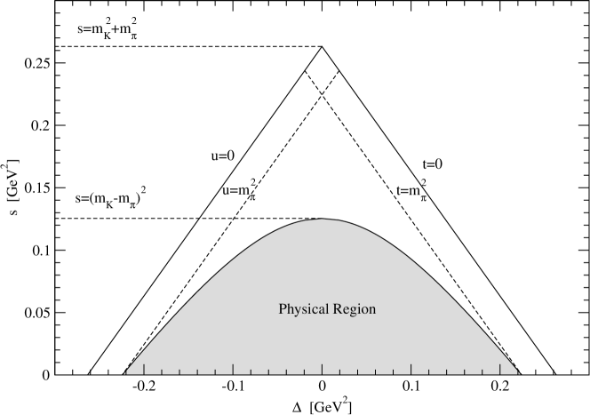
Figure 1: Dalitz plot for $K\to\pi\nu\bar{\nu}$.

Given the momenta $p_{K}$, $p_{\pi}$, $p_{\nu}$ and $p_{\bar{\nu}}$, one can define three Lorentz invariants

$$s=-(p_{K}-p_{\pi})^{2},\quad t=-(p_{K}-p_{\nu})^{2},\quad u=-(p_{K}-p_{\bar{\nu}})^{2},$$ (8)

where two of them are independent: $s+t+u=m_{K}^{2}+m_{\pi}^{2}$. Here we use a Euclidean metric with the signature (++++) so that an on-shell momentum is written as $p_{\pi}=(iE_{\pi},{\bf p}_{\pi})$ for a pion, and a minus sign appears in the definition for $s$, $t$ and $u$. Defining $\Delta\equiv u-t$, the physical region for $(\Delta,s)$ is denoted by the bounds

$$s\geq 0,\quad\Delta^{2}\leq(m_{K}^{2}+m_{\pi}^{2}-s)^{2}-4m_{K}^{2}m_{\pi}^{2}$$ (9)

and is illustrated in Fig. 1.

In our lattice calculation we take the kaon to be at rest so that $p_{K}=(im_{K},{\bf 0})$. The pion’s three-momentum is then given by

$$|{\bf p}_{\pi}|=\frac{\sqrt{s^{2}-2(m_{K}^{2}+m_{\pi}^{2})s+(m_{K}^{2}-m_{\pi}^{2})^{2}}}{2m_{K}}\,.$$ (10)

Without loss of generality, we choose the direction of the pion’s momentum to be ${\bf p}_{\pi}=\frac{|{\bf p}_{\pi}|}{\sqrt{3}}({\bf e}_{x}+{\bf e}_{y}+{\bf e}_{z})$, where ${\bf e}_{i}$ is the unit vector in the $i$-direction. We decompose the spatial momenta of the neutrino and anti-neutrino into components parallel and perpendicular to ${\bf p}_{\pi}$ writing

$${\bf p}_{\nu}={\bf p}_{\parallel}+{\bf p}_{\perp},\quad{\bf p}_{\bar{\nu}}=-{\bf p}_{\pi}-{\bf p}_{\parallel}-{\bf p}_{\perp}\,,$$ (11)

where ${\bf p}_{\parallel(\perp)}$ is parallel (perpendicular) to ${\bf p}_{\pi}$. The values of ${\bf p}_{\parallel}$ and ${\bf p}_{\perp}$ are given by

$${\bf p}_{\parallel} = -\frac{1}{2}\left\{\pm\frac{(m_{K}-E_{\pi})\Delta}{2m_{K}|{\bf p}_{\pi}|^{2}}+1\right\}\,{\bf p}_{\pi},$$

$${\bf p}_{\perp} = \frac{1}{2}\left\{s+\left(\frac{\Delta}{2m_{K}}\right)^{2}-\left(\frac{(m_{K}-E_{\pi})\Delta}{2m_{K}|{\bf p}_{\pi}|}\right)^{2}\right\}^{\frac{1}{2}}\,{\bf e}_{\perp},$$ (12)

where ${\bf e}_{\perp}$ is any unit vector perpendicular to ${\bf p}_{\pi}$. We use twisted boundary conditions to implement the momenta given by Eqs. (10) - (III.2).

Using the Dirac equation for the massless neutrinos, one can show that the magnitude of the decay amplitude vanishes at the edge of the physically-allowed region, where the momenta satisfy the condition $\Delta^{2}=(m_{K}^{2}+m_{\pi}^{2}-s)^{2}-4m_{K}^{2}m_{\pi}^{2}$. We are therefore more interested in momenta that are well inside the region and a natural choice is $(\Delta,s)=(0,0)$, which corresponds to the case in which the $\nu$ and $\bar{\nu}$ carry the same spatial momentum and the pion moves in the opposite direction with twice the momentum of each of the $\nu$ and $\bar{\nu}$. Since we perform the calculation at $m_{\pi}=420$ MeV, the allowed momenta for the final-state particles are constrained to lie in a small region. Given this small momentum range we expect that it will be be difficult to extract reliably the momentum dependence. For this reason, in this exploratory study we devote our computational resources to evaluating the amplitude at the single kinematical point with $(\Delta,s)=(0,0)$. The situation is expected to change once we perform the calculation at physical quark masses. In that case we will need to compute the $K^{+}\to\pi^{+}\nu\bar{\nu}$ amplitude at several values of $(\Delta,s)$ to gain a better understanding of the momentum dependence. Another consequence of the heavy pion mass is that the momenta of the pion and the neutrinos are very small. For $(\Delta,s)=(0,0)$ these are

$${\bf p}_{\nu}={\bf p}_{\bar{\nu}}=(0.0207,0.0207,0.0207),\quad{\bf p}_{\pi}=(-0.0414,-0.0414,-0.0414)\,.$$ (13)

Here $|{\bf p}_{\pi}|=0.0717$ is only about 18% of the lowest lattice momentum with periodic boundary conditions, $2\pi/L=0.3927$.

III.3 The bilocal operators

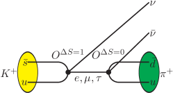
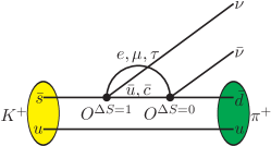
Type 1     Type 2 $W$-$W$ diagrams

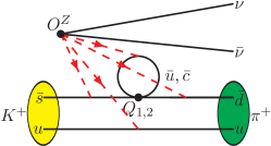
with self-loop     without self-loop connected $Z$-exchange diagrams

with self-loop     without self-loop disconnected $Z$-exchange diagrams

Figure 2: From top to bottom: quark and lepton contractions for $W$-$W$, connected and disconnected $Z$-exchange diagrams.

There are two classes of diagrams which contribute to $K^{+}\to\pi^{+}\nu\bar{\nu}$ decays, we call these the $W$-$W$ and $Z$-exchange diagrams. In the $W$-$W$ diagrams the second-order weak transition proceeds through the exchange of two $W$-bosons , while for the $Z$-exchange diagrams the decay occurs through the exchange of one $W$-boson and one $Z$-boson; both classes of diagrams are illustrated in Fig. 2. The bilocal contribution to the decay amplitude is a combination of these two types of diagrams so that it can be written in terms of the matrix element $\langle\pi^{+}\nu\bar{\nu}|{\mathcal{B}}(0)|K^{+}\rangle$, where the bilocal operator ${\mathcal{B}}(y)$ receives contributions from both ${\mathcal{B}}_{WW}(y)$ and ${\mathcal{B}}_{Z}(y)$

$${\mathcal{B}}(y)=\frac{G_{F}}{\sqrt{2}}\frac{\alpha}{2\pi\sin^{2}\theta_{W}}\frac{\pi^{2}}{M_{W}^{2}}\lambda_{c}\,\Big{(}{\mathcal{B}}_{WW}(y)+{\mathcal{B}}_{Z}(y)\Big{)}.$$ (14)

Here

$${\mathcal{B}}_{WW}(y)=\sum_{\ell=e,\mu,\tau}{\mathcal{B}}^{(\ell)}_{WW}(y),\quad{\mathcal{B}}_{Z}(y)=\sum_{\ell=e,\mu,\tau}{\mathcal{B}}^{(\ell)}_{Z}(y)$$ (15)

and ${\mathcal{B}}^{(\ell)}_{WW}(y)$ and ${\mathcal{B}}^{(\ell)}_{Z}(y)$ are defined as

$${\mathcal{B}}_{WW}^{(\ell)}(y)=\int d^{\hskip 1.5pt4}x\,T[O_{u\ell}^{\Delta S=1}(x)O_{u\ell}^{\Delta S=0}(y)]-\{u\to c\}$$ (16)

and

$${\mathcal{B}}_{Z}^{(\ell)}(y)=\int d^{\hskip 1.5pt4}x\,T[O_{u}^{W}(x)O_{\ell}^{Z}(y)]-\{u\to c\}.$$ (17)

Here, as in Ref. Bai et al. (2017); Christ et al. (2016a), we find it convenient to use the letter $O$ to represent an operator which incorporates a Wilson coefficient and the letter $Q$ for an operator which does not include such a coefficient. In Eq. (16) $O_{q\ell}^{\Delta S=1}$ and $O_{q\ell}^{\Delta S=0}$ are the appropriate products, $C_{A}^{\overline{\mathrm{MS}}}Q_{A}^{\overline{\mathrm{MS}}}$ and $C_{B}^{\overline{\mathrm{MS}}}Q_{B}^{\overline{\mathrm{MS}}}$, for the $W$-$W$ diagrams. We can write them in terms of bare lattice operators as

$$O_{q\ell}^{\Delta S=1}=Z_{V}\,(\bar{s}q)_{V-A}(\bar{\nu}\ell)_{V-A},\quad O_{q\ell}^{\Delta S=0}=Z_{V}\,(\bar{q}d)_{V-A}(\bar{\ell}\nu)_{V-A},$$ (18)

where $Z_{V}=Z_{A}$ is the renormalization factor relating the local lattice vector or axial-vector current (which we use) to the conserved or partially conserved ones and is effectively the corresponding Wilson coefficient. By taking the ratio of two-point functions computed with the local and conserved axial currents we obtain $Z_{A}=0.7163$, which is consistent with the result quoted in Ref. Aoki et al. (2008a).

The two effective operators for the $Z$-exchange diagrams are given by

$$O_{q}^{W}=C_{1}\,Q_{1,q}+C_{2}\,Q_{2,q},\quad O^{Z}_{\ell}=Z_{V}\,J_{\mu}^{Z}\,\big{[}\bar{\nu}_{\ell}\gamma^{\mu}(1-\gamma_{5})\nu_{\ell}\big{]}$$ (19)

with $Q_{1,q}$ and $Q_{2,q}$ the conventional current-current operators and $J_{\mu}^{Z}$ the quark current which couples to the $Z^{0}$. Their definition is given in Eq. (15) of Ref. Christ et al. (2016a), where a discussion of the corresponding operator renormalization from the lattice to the $\overline{\mathrm{MS}}$ scheme is also presented.

III.4 Matrix elements of local operators

In addition to the evaluation of the matrix elements of the bilocal operators discussed in Sec. III.3, which is the main task of this work, there are three types of matrix elements of local operators which must be computed in order to determine the $K^{+}\to\pi^{+}\nu\bar{\nu}$ decay amplitude.

• Matrix elements for the SD contributions, $\langle\pi^{+}\nu\bar{\nu}|Q_{0}|K^{+}\rangle$, for which the hadronic effects are obtained from matrix elements of the form $\langle\pi^{+}(\vec{p}_{f})|\bar{s}\gamma_{\mu}d|K^{+}(\vec{p}_{i})\rangle$. The labels $i$ and $f$ indicate the initial and final states, and are used to distinguish these states from the intermediate states discussed below.

• Matrix elements for low-lying intermediate states. This type of matrix element corresponds to unphysical contributions which grow exponentially in $T$, the time interval over which the separation of the two local operators $Q_{A}^{S}$ and $Q_{B}^{S}$ are integrated (see the discussion around Eq. (4)). Such terms arise when there are intermediate states whose energies are smaller than the kaon mass  Christ et al. (2016a). For the $W$-$W$ diagrams, see Fig. 2, we study the effects from the lowest two intermediate states: $|\bar{\ell}\nu\rangle$ and $|\pi^{0}\bar{\ell}\nu\rangle$. The unphysical contribution from the multi-hadron state $|\pi\pi\bar{\ell}\nu\rangle$ can be neglected due to phase space suppression. For the $Z$-exchange diagrams we examine and subtract the exponentially growing effects from $|\pi^{+}\rangle$ and $|(\pi^{+}\pi^{0})_{I=2}\rangle$ states, where $I$ is the total isospin of the two-pion state. Note that because of charge and angular momentum conservation only the $I=2$ $\pi\pi$ state can contribute to $Z$-exchange diagrams.

• Matrix elements of the local scalar density $\bar{s}d$, $\langle\pi^{+}|\bar{s}d|K^{+}\rangle$. Since the scalar density operator does not contribute to the on-shell matrix element, we can shift the effective Hamiltonian by $H_{W}\to H_{W}^{\prime}=H_{W}-c_{s}\,\bar{s}d$ without changing the amplitude Christ et al. (2013). By choosing an appropriate value for $c_{s}$ we remove the unphysical contribution from the $|\pi^{+}\rangle$ intermediate state in the $Z$-exchange diagrams. We will discuss this in more detail in the following sections. In other applications, one also frequently subtracts a term proportional to the pseudoscalar density from the effective Hamiltonian to remove a low-lying state from the correlation function. However, in this case there is no contribution from the vacuum state and the operator $\bar{s}\gamma^{5}d$ cannot mediate transitions to $I=2$ two-pion states (by isospin conservation). We therefore do not make the subtraction $H_{W}\to H_{W}^{\prime}=H_{W}-c_{p}\,\bar{s}\gamma^{5}d$ here.

The three types of hadronic matrix elements are summarized in Table 1 and will be used below for the analysis of the second-order weak transition amplitude. We now proceed to a discussion of the evaluation of the matrix elements of these local operators.

Matrix element for the SD contribution
$Q_{0}$	$\langle\pi^{+}\nu\bar{\nu}|Q_{0}|K^{+}\rangle$	$\langle\pi^{+}(\vec{p}_{f})|\bar{s}\gamma_{\mu}d|K^{+}(\vec{p}_{i})\rangle$
Matrix element relevant for low-lying intermediate states
$W$-$W$	$\langle\pi^{+}\nu\bar{\nu}|O_{u}^{\Delta S=0}|\bar{\ell}\nu\rangle\langle\bar{\ell}\nu|O_{u}^{\Delta S=1}|K^{+}\rangle$	$\langle\pi^{+}(\vec{p}_{f})|\bar{u}\gamma_{\mu}\gamma_{5}d|0\rangle$, $\langle 0|\bar{s}\gamma_{\mu}\gamma_{5}u|K^{+}(\vec{p}_{i})\rangle$
	$\langle\pi^{+}\nu\bar{\nu}|O_{u}^{\Delta S=0}|\pi^{0}\bar{\ell}\nu\rangle\langle\pi^{0}\bar{\ell}\nu|O_{u}^{\Delta S=1}|K^{+}\rangle$	$\langle\pi^{+}(\vec{p}_{f})|\bar{u}\gamma_{\mu}d|\pi^{0}\rangle$, $\langle\pi^{0}|\bar{s}\gamma_{\mu}u|K^{+}(\vec{p}_{i})\rangle$
$Z$-exchange	$\langle\pi^{+}\nu\bar{\nu}|O_{\ell}^{Z}|\pi^{+}\rangle\langle\pi^{+}|O_{q}^{W}|K^{+}\rangle$	$\langle\pi^{+}(\vec{p}_{f})|\bar{u}\gamma_{\mu}u|\pi^{+}\rangle$, $\langle\pi^{+}(\vec{p}_{f})|\bar{d}\gamma_{\mu}d|\pi^{+}\rangle$
		$\langle\pi^{+}|Q_{1,q}|K^{+}(\vec{p}_{i})\rangle$, $\langle\pi^{+}|Q_{2,q}|K^{+}(\vec{p}_{i})\rangle$
	$\langle\pi^{+}\nu\bar{\nu}|O_{\ell}^{Z}|(\pi^{+}\pi^{0})_{I=2}\rangle\langle(\pi^{+}\pi^{0})_{I=2}|O_{q}^{W}|K^{+}\rangle$	$\langle\pi^{+}(\vec{p}_{f})|\bar{u}\gamma_{\mu}\gamma_{5}u|(\pi^{+}\pi^{0})_{I=2}\rangle$
		$\langle\pi^{+}(\vec{p}_{f})|\bar{d}\gamma_{\mu}\gamma_{5}d|(\pi^{+}\pi^{0})_{I=2}\rangle$
		$\langle(\pi^{+}\pi^{0})_{I=2}|Q_{1,u}|K^{+}(\vec{p}_{i})\rangle$
		$\langle(\pi^{+}\pi^{0})_{I=2}|Q_{2,u}|K^{+}(\vec{p}_{i})\rangle$
Matrix element for the shift in the Hamiltonian
$Z$-exchange	$H_{W}\to H_{W}-c_{s}\,\bar{s}d$	$\langle\pi^{+}|\bar{s}d|K^{+}(\vec{p}_{i})\rangle$

Table 1: Hadronic matrix elements of local operators required for the calculation of the $K^{+}\to\pi^{+}\nu\bar{\nu}$ amplitude (third column). $\vec{p}_{i}$ and $\vec{p}_{f}$ are the momenta of the initial state kaon and final state pion, whereas the momenta of the intermediate states are not shown explicitly. The second column includes the neutrinos and for the $W$-$W$ and $Z$-exchange diagrams displays the corresponding contributions to the bilocal matrix elements.

III.4.1 Correlators and propagators

In Table 1, except for the matrix elements $\langle\pi^{+}(\vec{p}_{f})|\bar{u}\gamma_{\mu}\gamma_{5}d|0\rangle$ and $\langle 0|\bar{s}\gamma_{\mu}\gamma_{5}u|K^{+}(\vec{p}_{i})\rangle$ which are proportional to the the leptonic decay constants and can be determined from 2-point correlation functions, the remaining matrix elements of local operators can be extracted from 3-point correlation functions of the general form $\langle\phi_{A}(t_{A})\,O(t_{O})\,\phi_{B}^{\dagger}(t_{B})\rangle$, where $\phi_{A}$ and $\phi^{\dagger}_{B}$ are interpolating operators which can annihilate hadron A or create hadron B. We define the quantity

$$\mathcal{M}_{AOB}(t_{A},t_{O},t_{B})=\frac{2E_{A}\,2E_{B}}{N_{A}\,N_{B}^{\dagger}}\langle\phi_{A}(t_{A})O(t_{O})\phi_{B}^{\dagger}(t_{B})\rangle e^{E_{A}(t_{A}-t_{O})}e^{E_{B}(t_{O}-t_{B})},$$ (20)

where we do not exhibit the dependence of the operators on the spatial coordinates. Here $A$ and $B$ indicate initial-, intermediate- or final-state particles, i.e. $K^{+}$, $\pi^{+,0}$ and $(\pi^{+}\pi^{0})_{I=2}$. We use Coulomb gauge-fixed wall sources for the $\phi_{A}$ and $\phi_{B}$ interpolating operators. Such wall-source operators have a good overlap with the $\pi$, $K$ and $(\pi^{+}\pi^{0})_{I=2}$ ground states. The coefficients $N_{A}$ and $N_{B}$ can be extracted from the corresponding 2-point correlation functions using the same wall-source operators. $E_{A}$ and $E_{B}$ are the ground-state energies which can also be determined from 2-point functions. The matrix element $\langle A|O|B\rangle=\mathcal{M}_{AOB}(t_{A},t_{O},t_{B})$ can then be determined from the three-point correlation functions using Eq. (20) at large $t_{A}-t_{O}\gg 0$ and $t_{O}-t_{B}\gg 0$.

In Eq. (20) the operator $O$ can be a vector or axial-vector current, the current-current operators $Q_{1q}$ and $Q_{2q}$ or the scalar density $\bar{s}d$. The interpolating operators $\phi_{A,B}$ are constructed using twisted boundary conditions to ensure that the corresponding states have the required momenta. Translation invariance then implies that the correlation functions in Eq.( 20) do not depend on the spatial position $\vec{x}$ of the operator $O(t_{O},\vec{x}\,)$. In order to obtain a better precision we treat $\vec{x}$ as the sink of the quark propagators and sum over $\vec{x}$ with the appropriate phase factor to account for the momentum transfer between states $A$ and $B$. The resulting volume factor in the 3-point function cancels with that from the 2-point functions used to determine $N_{A}$ and $N_{B}$.

The operators $Q_{1,q}$ and $Q_{2,q}$ can induce closed quark loops in the contractions. We therefore need to calculate the light and charm quark propagators $D^{-1}_{u,c}(x,x)$ for all possible $x$ and using random-source propagators is a natural way to evaluate these quark loops Christ et al. (2016e). For a similar cost, one can either put one random wall source at each of the $T$ time slices or use $N_{r}=T$ random volume sources with no dilution in the time slices. Although the cost of these two choices is almost the same, the latter one reduces the error by a factor of $1.5$ compared to the former. We thus use $N_{r}=T=32$ random volume source propagators to calculate the light and charm quark propagator $D^{-1}_{u,c}(x,x)$ for all possible $x$. We also make use of the time translation invariance and average the correlator over all $T$ time translations

$$\bar{\mathcal{M}}_{AOB}(t_{2},t_{1})=\frac{1}{T}\sum_{t=0}^{T-1}{\mathcal{M}}_{AOB}(t_{2}+t,t_{1}+t,t).$$ (21)

By doing this, our results show that the statistical error can be efficiently reduced by nearly a factor of $\sqrt{T}$. The time translation average requires the wall-source propagators to be generated on all time slices. This can be achieved in an efficient way by calculating the low-lying eigenvectors of the Dirac operator using the Lanczos method and then using low-mode deflation to accelerate the light-quark inversions. Working on the $16^{3}\times 32$ lattice, we find that by using 100 eigenvectors in low-mode deflation the light-quark conjugate gradient (CG) time is reduced to 16% of that required for the CG inversions without low-mode deflation.

III.4.2 Exploiting isospin symmetry to simplify the derivation of the contractions

Since this computation is performed in the isospin-symmetric limit, we can exploit this symmetry to derive the necessary contractions more readily. For example, we have the following relations between the matrix elements:

$$\langle\pi^{0}|\bar{s}\gamma_{\mu}u|K^{+}\rangle = \frac{1}{\sqrt{2}}\langle\pi^{+}|\bar{s}\gamma_{\mu}d|K^{+}\rangle$$

$$\langle\pi^{+}|\bar{u}\gamma_{\mu}d|\pi^{0}\rangle = \sqrt{2}\langle\pi^{+}|\bar{d}\gamma_{\mu}d|\pi^{+}\rangle$$ (22)

$$\langle\pi^{+}|\bar{u}\gamma_{\mu}\gamma_{5}u-\bar{d}\gamma_{\mu}\gamma_{5}d|(\pi^{+}\pi^{0})_{I=2}\rangle = \langle\pi^{+}|\bar{d}\gamma_{\mu}\gamma_{5}u|(\pi^{+}\pi^{+})_{I=2}\rangle.$$

The matrix elements on the right-hand side have simpler contractions since they do not involve the neutral pion, the $\pi^{0}$. More precisely, although the final set of contractions is of course the same, by using the relations in Eqs. (22) there are fewer cancelations of diagrams in intermediate steps of the calculation.

We now express some of the matrix elements in Table 1 in terms of invariant form factors:

$$Z_{V}\langle\pi^{+}(p_{\pi})|\bar{s}\gamma_{\mu}d|K^{+}(p_{K})\rangle = i\left\{\,(p_{K}+p_{\pi})_{\mu}f_{+}(s)+(p_{K}-p_{\pi})_{\mu}f_{-}(s)\,\right\}$$ (23)

$$(m_{s}-m_{d})\langle\pi^{+}(p_{\pi})|\bar{s}d|K^{+}(p_{K})\rangle = (m_{K}^{2}-m_{\pi}^{2})f_{0}(s)$$ (24)

$$Z_{V}\langle\pi^{+}(p_{2})|\bar{d}\gamma_{\mu}d|\pi^{+}(p_{1})\rangle = i\,F_{\pi}(s)(p_{1}+p_{2})_{\mu}\,,$$ (25)

where $s=-(p_{K}-p_{\pi})^{2}$ for the $K_{\ell 3}$ form factors $f_{+,-,0}(s)$ and $s=-(p_{1}-p_{2})^{2}$ for the pion form factor $F_{\pi}(s)$. In Eqs. (23) and (25), $Z_{V}$ is the renormalization constant relating the local vector current to the conserved one. The momentum $p_{i}$ is a Euclidean four-momentum defined as $p_{i}=(iE_{i},{\bf p}_{i})$ with $E_{i}$ and ${\bf p}_{i}$ the energy and spatial momentum of the corresponding on-shell particle. The scalar form factor is a linear combination of $f_{+}(s)$ and $f_{-}(s)$:

$$f_{0}(s)=f_{+}(s)+\frac{s}{m_{K}^{2}-m_{\pi}^{2}}f_{-}(s)\,,$$ (26)

which follows from Eqs. (23) and (24) and a chiral Ward identity.

The current-current operators $Q_{i,u}$ in Eq. (19) are linear combinations of $\Delta I=3/2$ and $\Delta I=1/2$ operators. Only the $\Delta I=3/2$ component contributes to the $K^{+}\to(\pi^{+}\pi^{0})_{I=2}$ transition. For the $K\to(\pi\pi)_{I=2}$ transition we have

$$\langle(\pi^{+}\pi^{0})_{I=2}|Q_{i,u}|K^{+}\rangle=\frac{1}{\sqrt{3}}\langle(\pi^{+}\pi^{0})_{I=2}|Q^{\Delta I=\frac{3}{2},\Delta I_{z}=\frac{1}{2}}|K^{+}\rangle,\quad i=1,2$$ (27)

where the operator with isospin $\Delta I=3/2$, $\Delta I_{z}=1/2$ is given by

$$Q^{\Delta I=\frac{3}{2},\Delta I_{z}=\frac{1}{2}}=\frac{1}{\sqrt{3}}\left(-(\bar{s}d)_{V-A}(\bar{d}d)_{V-A}+(\bar{s}d)_{V-A}(\bar{u}u)_{V-A}+(\bar{s}u)_{V-A}(\bar{u}d)_{V-A}\right).$$ (28)

One can now use the Wigner-Eckhart theorem for isospin symmetry and write the matrix element for the $K\to(\pi^{+}\pi^{0})_{I=2}$ decay in terms of that into the maximally extended state $|\pi^{+}\pi^{+}\rangle$:

$$\langle(\pi^{+}\pi^{0})_{I=2}|Q_{i,u}|K^{+}\rangle=\frac{1}{2}\langle(\pi^{+}\pi^{+})_{I=2}|(\bar{s}d)_{V-A}(\bar{u}d)_{V-A}|K^{+}\rangle,$$ (29)

where $(\bar{s}d)_{V-A}(\bar{u}d)_{V-A}$ is a $\Delta I=3/2$, $\Delta I_{z}=3/2$ operator. The determination of the necessary contractions is simpler using the matrix element for the $K^{+}\to(\pi^{+}\pi^{+})_{I=2}$ decay than for the $K^{+}\to(\pi^{+}\pi^{0})_{I=2}$ transition. (Note that Eq. (29) was used throughout the RBC-UKQCD collaborations’ computations of the $\Delta I=\frac{3}{2},\,K\to\pi\pi$ amplitude $A_{2}$ Blum et al. (2012a, b, 2015). The motivation in Refs. Blum et al. (2012a, b, 2015) was different however; there it was to use antiperiodic boundary conditions on the $u$ quark to match the $I=2$, $\pi\pi$ ground-state energy to the mass of the kaon, $m_{K}$.)

III.4.3 Around-the-world effects

To extract the matrix elements one needs to determine the coefficients $N_{A}$ and $N_{B}$ for $A,B=K^{+},\pi^{+,0},(\pi^{+}\pi^{0})_{I=2}$. For the case when $A=B=(\pi^{+}\pi^{0})_{I=2}$ one has to consider the subtlety of round-the-world effects. The corresponding two-point function is given by

$$C_{\pi\pi}(t)=\langle\phi_{\pi\pi}(t)\phi_{\pi\pi}^{\dagger}(0)\rangle\xrightarrow[]{T\gg t\gg 0}\frac{N_{\pi\pi}^{2}}{2E_{\pi\pi}}\left(e^{-E_{\pi\pi}t}+e^{-E_{\pi\pi}(T-t)}\right)+N_{0}(T).$$ (30)

Here an unwanted term, $N_{0}(T)$ (proportional to $e^{-E_{\pi}T}$ where $E_{\pi}$ is the energy of a single pion), is induced by the around-the-world effects in which each of $\phi_{\pi\pi}$ interpolating operators in Eq. (30) creates one pion and annihilates another. We can remove this term by performing the subtraction through

$$C_{\pi\pi}(t)-C_{\pi\pi}(t+1)=\frac{N_{\pi\pi}^{2}}{2E_{\pi\pi}}\left(-4e^{-\frac{E_{\pi\pi}}{2}T}\right)\sinh(E_{\pi\pi}t^{\prime})\sinh\frac{E_{\pi\pi}}{2}.$$ (31)

where $t^{\prime}=t+1/2-T/2$. For the single-pion 2-point function, $C_{\pi}(t)$, where the pion has energy $E_{\pi}$, we have

$$C_{\pi}^{2}(t)-C_{\pi}^{2}(t+1)=\frac{N_{\pi}^{4}}{(2E_{\pi})^{2}}\left(-4e^{-E_{\pi}T}\right)\sinh(2E_{\pi}t^{\prime})\sinh E_{\pi}\,.$$ (32)

By constructing the ratio $R(t+\frac{1}{2})\equiv\frac{C_{\pi\pi}(t)-C_{\pi\pi}(t+1)}{C_{\pi}^{2}(t)-C_{\pi}^{2}(t+1)}$, we can determine $N_{\pi\pi}$ and $\delta E\equiv E_{\pi\pi}-2E_{\pi}$ from Feng et al. (2010)

$$R(t+1/2) = A_{R}\left(\cosh(\delta E\,t^{\prime})+\sinh(\delta E\,t^{\prime})\coth(2E_{\pi}\,t^{\prime})\right),\quad\textrm{where}$$

$$A_{R} = \frac{N_{\pi\pi}^{2}}{2E_{\pi\pi}}\frac{(2E_{\pi})^{2}}{N_{\pi}^{4}}e^{-\frac{\delta E}{2}T}\frac{\sinh\frac{E_{\pi\pi}}{2}}{\sinh E_{\pi}}.$$ (33)

At threshold (i.e. with $E_{\pi}=m_{\pi}$) we obtain $\delta E=0.01803(32)$ from which, using Lüscher’s finite-size formula Luscher (1986), we find $m_{\pi}a_{\pi\pi}=-0.2816(43)$, where $a_{\pi}$ is the $\pi$-$\pi$ scattering length. This result is close to the estimate $m_{\pi}a_{\pi\pi}^{\mathrm{LO}}=-\frac{m_{\pi}^{2}}{8\pi f_{\pi}^{2}}=-0.2978(23)$ from leading-order chiral perturbation theory (ChPT) Weinberg (1966). Here we have used the values $am_{\pi}=0.24360(47)$ and $af_{\pi}=0.08904(19)$ from our simulation. The difference between the values deduced from $\delta E$ and LO ChPT is expected to be due to higher-order terms in ChPT, as well as to possible systematic effects.

III.4.4 Lattice results

Matrix elements for the SD contribution
$\langle\pi^{+}(p)|\bar{s}\gamma_{i}d|K^{+}(0)\rangle$	$-i\leavevmode\nobreak\ 0.06014(77)$	$f_{+}(s)$	$0.993(3)$
$\langle\pi^{+}(p)|\bar{s}\gamma_{t}d|K^{+}(0)\rangle$	$-0.7970(14)$	$f_{-}(s)$	$-0.048(12)$
		$f_{0}(s)$	$0.993(3)$
$\langle\pi^{+}(0)|\bar{s}\gamma_{t}d|K^{+}(0)\rangle$	$-0.7992(15)$	$f_{0}(s_{\mathrm{max}})$	$1.006(3)$
Matrix elements relevant for the contributions of low-lying intermediate states
$W$-$W$
$\langle\pi^{0}(0)|\bar{s}\gamma_{t}u|K^{+}(0)\rangle$	$-0.7992(15)$	$f_{0}(s_{\mathrm{max}})$	$1.006(3)$
$\langle\pi^{+}(p)|\bar{u}\gamma_{i}d|\pi^{0}(0)\rangle$	$-i\leavevmode\nobreak\ 0.05612(62)$	$F_{\pi}(s)$	$0.971(11)$
$\langle\pi^{+}(p)|\bar{u}\gamma_{t}d|\pi^{0}(0)\rangle$	$-0.6830(15)$	$F_{\pi}(s)$	$0.986(2)$
$Z$-exchange
$\langle\pi^{+}(0)|Q_{1,q}|K^{+}(0)\rangle$	$1.697(87)\times 10^{-4}$	$c_{s}^{(1)}$	$0.795(41)\times 10^{-4}$
$\langle\pi^{+}(0)|Q_{2,q}|K^{+}(0)\rangle$	$3.828(98)\times 10^{-4}$	$c_{s}^{(2)}$	$1.794(46)\times 10^{-4}$
$\langle(\pi^{+}\pi^{0})_{I=2}(0)|Q_{i,q}|K^{+}(0)\rangle$	$-i\leavevmode\nobreak\ 4.165(18)\times 10^{-4}$
$\langle\pi^{+}(0)|\bar{u}\gamma_{t}\gamma_{5}u-\bar{d}\gamma_{t}\gamma_{5}d|(\pi^{+}\pi^{0})_{I=2}(0)\rangle$	$i\leavevmode\nobreak\ 2.4930(84)$
Matrix element for the subtraction in the effective Hamiltonian
$\langle\pi^{+}(0)|\bar{s}d|K^{+}(0)\rangle$	$2.1335(58)$	$f_{0}(s_{\mathrm{max}})$	$1.007(2)$

Table 2: Lattice results for the local matrix elements. The state $|\pi^{+}(p)\rangle$ denotes a $\pi^{+}$ with momentum $p=|{\bf p}_{\pi}|$ where ${\bf p}_{\pi}$ given in Eq. (13). For the matrix element $\langle\pi^{+}(p)|\bar{s}\gamma_{\mu}d|K^{+}(0)\rangle$, $s=(m_{K}-E_{\pi})^{2}-p^{2}$ whereas for $\langle\pi^{+}(p)|\bar{u}\gamma_{\mu}d|\pi^{0}(0)\rangle$, $s=(E_{\pi}-m_{\pi})^{2}-p^{2}$. Similarly, when the $\pi^{+,0}$ in the intermediate state is at rest, $s=s_{\textrm{max}}=(m_{K}-m_{\pi})^{2}$. The matrix elements $\langle(\pi^{+}\pi^{0})_{I=2}(0)|Q_{1,q}|K^{+}(0)\rangle$ and $\langle(\pi^{+}\pi^{0})_{I=2}(0)|Q_{2,q}|K^{+}(0)\rangle$ are equal.

Consider the time-dependent amplitude $\bar{\mathcal{M}}_{AOB}(t_{2},t_{1},0)$ defined in Eq. (21). We require $t_{2}-t_{1}$ and $t_{1}-0$ to be sufficiently large to suppress the contamination from excited states and $t_{2}\ll T$ to suppress around-the-world effects. In practice we define $\mathcal{M}_{AOB}^{\mathrm{mid}}(t)\equiv\bar{\mathcal{M}}_{AOB}(t,\frac{t}{2},0)$ (or if $t$ is odd, then $\mathcal{M}_{AOB}^{\mathrm{mid}}(t)\equiv\frac{1}{2}[\bar{\mathcal{M}}_{AOB}(t,\frac{t-1}{2},0)+\bar{\mathcal{M}}_{AOB}(t,\frac{t+1}{2},0)]$) and choose appropriate values for $t$ to control both the excited-state and around-the-world effects. By studying the $t$ dependence of $\mathcal{M}_{AOB}^{\mathrm{mid}}(t)$ we determine the local matrix element $\langle A|O|B\rangle$ and present the corresponding results in Table 2. In the table we present the values of the $K\to\pi$, $\pi\to\pi$, $K\to(\pi^{+}\pi^{0})_{I=2}$ and $(\pi^{+}\pi^{0})_{I=2}\to\pi$ matrix elements required for the analysis, and in particular for the subtraction of the exponentially growing contributions from low-lying states. Although in this simulation $m_{K}<2m_{\pi}$, so that there are no exponentially growing contributions from two-pion intermediate states, we include below an explicit discussion of the $|(\pi^{+}\pi^{0})_{I=2}\rangle$ state and the evaluation of the corresponding matrix elements in preparation for simulations with physical quark masses for which $m_{K}>2m_{\pi}$. In the final two columns of Table 2 we present the $K_{\ell 3}$ form factors $f_{+}(s)$, $f_{-}(s)$ and $f_{0}(s)$, the pion form factors $F_{\pi}(s)$, and the coefficient $c_{s}^{(i)}$ from the ratio $c_{s}^{(i)}=\frac{\langle\pi|Q_{i,q}|K\rangle}{\langle\pi|\bar{s}d|K\rangle}$. We determine $f_{0}(s_{\mathrm{max}})$ with $s_{\mathrm{max}}=(m_{K}-m_{\pi})^{2}$ from both $\langle\pi^{+}(0)|\bar{s}\gamma_{t}d|K^{+}(0)$ and $\langle\pi^{+}(0)|\bar{s}d|K^{+}(0)$ and obtain consistent results. The matrix element $\langle\pi^{+}(p)|\bar{u}\gamma_{\mu}d|\pi^{0}(0)\rangle$ yields consistent results for $F_{\pi}(s)$ from the spatial and temporal polarization directions, although the former one is much noisier.

For the $\pi^{+}\pi^{0}$ contribution to the $Z$-exchange diagrams, we determine the matrix element $\langle\pi^{+}(0)|(\bar{u}\gamma_{t}\gamma_{5}u-\bar{d}\gamma_{t}\gamma_{5}d)|(\pi^{+}\pi^{0})_{I=2}(0)\rangle=i\leavevmode\nobreak\ 2.4930(84)$ by performing the isospin rotation $(\pi^{+}\pi^{0})_{I=2}\to(\pi^{+}\pi^{+})_{I=2}$ in Eq. (III.4.2). Here the two-pions are in the ground state, i.e. at threshold. This value of the matrix element is only about 8% smaller than an estimate from tree level chiral perturbation theory, where the interaction between the two pions in the I=2 state is neglected.

III.5 Evaluation of the matrix element of the bilocal operator for the $W$-$W$ diagrams

In this section we discuss the evaluation of the matrix element of the bilocal operator ${\mathcal{B}}_{WW}(y)$ defined in Eq. (16). The matrix element $T_{WW}$ for the $W$-$W$ diagrams is given by

$$T_{WW}=\int d^{4}x\,\langle\pi^{+}\nu\bar{\nu}|T\{O_{u\ell}^{\Delta S=1}(x)O_{u\ell}^{\Delta S=0}(y)\}|K^{+}\rangle-\{u\to c\}\,.$$ (34)

As explained in Ref. Christ et al. (2016a), $T_{WW}$ can be written in terms of the scalar amplitude $F_{WW}(\Delta,s)$ and leptonic spinor product $\bar{u}(p_{\nu}){\not{p}}_{K}(1-\gamma_{5})v(p_{\bar{\nu}})$:

$$T_{WW}=i\leavevmode\nobreak\ F_{WW}(\Delta,s)\,\left[\bar{u}(p_{\nu}){\not{p}}_{K}(1-\gamma_{5})v(p_{\bar{\nu}})\right],$$ (35)

where the variables $\Delta$ and $s$ are defined in the paragraph following Eq. (8). In practice one can obtain $F_{WW}(\Delta,s)$ through Christ et al. (2016a)

$$F_{WW}(\Delta,s)=-i\int d^{4}x\,H_{\alpha\beta}(x,y)\sum_{\mu}c_{\mu}\mathrm{Tr}\left[\Gamma_{\alpha\beta}(x,y)\gamma_{\mu}(1+\gamma_{5})\right]\,,$$ (36)

where the coefficient $c_{\mu}$ is given by

$$c_{\mu}=\frac{1}{8}\frac{b_{\mu}}{b\cdot p_{K}}\quad\textrm{where}\quad b_{\mu}=\frac{1}{4}\mathrm{Tr}\left[\gamma_{\mu}{\not{p}}_{\bar{\nu}}{\not{p}}_{K}(1-\gamma_{5}){\not{p}}_{\nu}\right].$$ (37)

The hadronic and leptonic parts, $H_{\alpha\beta}(x,y)$ and $\Gamma_{\alpha\beta}(x,y)$, are defined by

$$H_{\alpha\beta}(x,y) = Z_{V}^{2}\langle\pi^{+}(p_{\pi})|T[\bar{s}\gamma_{\alpha}(1-\gamma_{5})u(x)\,\bar{u}\gamma_{\beta}(1-\gamma_{5})d(y)]|K^{+}(p_{K})\rangle-\{u\to c\}$$

$$\Gamma_{\alpha\beta}(x,y) = \gamma_{\alpha}(1-\gamma_{5})S_{\ell}(x,y)\gamma_{\beta}(1-\gamma_{5})e^{-ip_{\nu}x}e^{-ip_{\bar{\nu}}y}\,,$$ (38)

where $S_{\ell}(x,y)$ is the free lepton propagator for $\ell=e,\mu$ or $\tau$.

III.5.1 Construction of the correlation function

Similarly to the calculation of the matrix elements of local operators, we use Coulomb-gauge wall-source interpolating operators to create the kaon in the initial state and the pion in the final state. For the two weak operators $O_{q\ell}^{\Delta S=1}(x)$ and $O_{q\ell}^{\Delta S=0}(y)$, one is evaluated at a fixed point which is used as the source for the internal quark lines connected to that operator. The second operator acts as the sink for all the propagators joined to it and is summed over the spatial volume. To gain a higher precision from the time translation average, we calculate the point source propagators at all $T$ time slices. We also exchange the source and sink locations between the two weak operators and average over both choices.

III.5.2 Lepton propagator with infinite time extent

A subtlety in the calculation of the $W$-$W$ diagrams is the inclusion of the lepton propagators, $S_{\ell}(x,y)$. For the light leptons $\ell=e,\mu$ the round-the-world effects are significant in our lattice calculation with temporal extent $T=32$. To solve this problem, we first write the lepton propagator in the spatial momentum-time mixed representation

$$S_{\ell}^{(T)}({\bf p},t)=\frac{1}{T}\sum_{p_{4}}S_{\ell}({\bf p},p_{4})e^{ip_{4}t},\quad p_{4}=\frac{2\pi}{T}n,\quad n=0,1,\cdots T-1,$$ (39)

where $S_{\ell}({\bf p},p_{4})$ is the lepton propagator in momentum space. We then construct the propagator with infinite time extent as

$$S_{\ell}^{(\infty)}({\bf p},t)\equiv\int_{-\pi}^{\pi}\frac{dp_{4}}{2\pi}S_{\ell}({\bf p},p_{4})e^{ip_{4}t}.$$ (40)

Instead of using $S_{\ell}^{(T)}({\bf p},t)$ with periodic boundary condition we use the time-truncated lepton propagator $S_{\ell}^{[T]}({\bf p},t)$ to avoid round-the-world effects

$$S_{\ell}^{[T]}({\bf p},t)\equiv\begin{cases}S_{\ell}^{(\infty)}({\bf p},t)&\mbox{for $-T/2\leq t<T/2$}\\ 0&\mbox{for $t\geq T/2$ or $t<-T/2$}\end{cases}.$$ (41)

Such a time-truncated lepton propagator is implemented using an overlap fermion formulation. The detailed expression of $S_{\ell}^{[T]}({\bf p},t)$ can be found in Appendix A.

III.5.3 Using twisted boundary conditions to insert momenta

In the present computation, the kaon is at rest, while the pion, neutrino and anti-neutrino in the final state have nonzero momenta as indicated by Eq. (13). We therefore use twisted boundary conditions for the $d$ quark to insert the nonzero momentum ${\bf p}_{\pi}$ for the pion in the final state. Spatial momentum conservation implies that in the process $K^{+}\to(\ell^{+}X)^{*}\nu\to\pi^{+}\nu\bar{\nu}$, the intermediate state $(\ell^{+}X)^{*}$ has the nonzero momentum ${\bf p}_{K}-{\bf p_{\nu}}$. Here the superscript ^∗ indicates that the particles are off-shell and $X$ represents hadrons or the vacuum. We use twisted boundary conditions for the lepton field and periodic boundary condition for internal up and charm quark fields. In this way, the lepton $\ell^{+}$ has momentum ${\bf p}_{\ell}={\bf p}_{K}-{\bf p}_{\nu}+\frac{2\pi}{L}{\bf n}$, where ${\bf n}=(n_{1},n_{2},n_{3})$, $n_{i}\in\{0,1,\cdots,L-1\}$, and the hadronic particles $X$ have a total spatial momentum ${\bf p}_{X}=-\frac{2\pi}{L}{\bf n}$. For the intermediate ground state ${\bf p}_{\ell}={\bf p}_{K}-{\bf p}_{\nu}$ and ${\bf p}_{X}={\bf 0}$.

III.5.4 Exponentially growing unphysical terms

In the evaluation of integrals of matrix elements of bilocal operators over a large, but finite Euclidean time interval, there exist unphysical terms which grow exponentially as the range of the time integration is increased. Given the bilocal matrix element $\int d^{4}x\,\langle\pi^{+}\nu\bar{\nu}|T[O^{\Delta S=1}(x)O^{\Delta S=0}(0)]|K^{+}\rangle$, one can insert a complete set of intermediate states between the two interpolating operators, $O^{\Delta S=1}$ and $O^{\Delta S=0}$. Integrating over an interval of $-T_{a}<x_{0}<T_{b}$ ($T_{a},T_{b}>0$) gives

$$\int_{-T_{a}}^{T_{b}}dx_{0}\int d^{3}\vec{x}\,\langle\pi^{+}\nu\bar{\nu}|T[O^{\Delta S=1}(x)O^{\Delta S=0}(0)]|K^{+}\rangle =$$ (42)

$$\sum_{n_{s}}\cfrac{\langle\pi^{+}\nu\bar{\nu}|O^{\Delta S=1}|n_{s}\rangle\langle n_{s}|O^{\Delta S=0}|K^{+}\rangle}{E_{n_{s}}-E_{K}}\left(1-e^{(E_{K}-E_{n_{s}})T_{b}}\right)$$

$$-\sum_{n}\cfrac{\langle\pi^{+}\nu\bar{\nu}|O^{\Delta S=0}|n\rangle\langle n|O^{\Delta S=1}|K^{+}\rangle}{E_{K}-E_{n}}\left(1-e^{(E_{K}-E_{n})T_{a}}\right).$$

The second and third lines of Eq. (42) give the second-order weak matrix element together with the unwanted exponential terms. For the intermediate states $|n\rangle=|\ell^{+}\nu\rangle$ and $|\pi^{0}\ell^{+}\nu\rangle$, the factor $e^{(E_{K}-E_{n})T_{a}}$ increases exponentially as $T_{a}$ increases. We have determined the hadronic matrix elements $\langle\pi^{+}|\bar{s}\gamma_{\mu}\gamma_{5}d|0\rangle$ and $\langle 0|\bar{s}\gamma_{\mu}\gamma_{5}u|K^{+}\rangle$ from 2-point correlation functions and $\langle\pi^{+}|\bar{u}\gamma_{\mu}d|\pi^{0}\rangle$ and $\langle\pi^{0}|\bar{s}\gamma_{\mu}u|K^{+}\rangle$ from 3-point correlation functions (see Table 2 for the results). Therefore we can remove these exponentially growing terms directly. At $m_{\pi}=420$ MeV, the exponential terms from the states $|n\rangle=|\pi\pi\ell^{+}\nu\rangle$ and $|3\pi\ell^{+}\nu\rangle$ vanish at large $T_{a}$. At the physical pion mass, although the unphysical terms from $|\pi\pi\ell^{+}\nu\rangle$ and $|3\pi\ell^{+}\nu\rangle$ grow exponentially at large $T_{a}$, they are significantly suppressed by phase space and are expected to be negligible in lattice QCD calculations Christ et al. (2016a).

III.5.5 Double integration method

Since the point-source propagators are placed on each time slice, we can adopt the method proposed in Ref. Christ et al. (2013) and perform the time integral over the time locations of both $O_{q\ell}^{\Delta S=1}$ and $O_{q\ell}^{\Delta S=0}$

$$\sum_{t_{1}=t_{a}}^{t_{b}}\sum_{t_{2}=t_{a}}^{t_{b}}\int d^{3}{\bf x}\,\langle\pi^{+}\nu\bar{\nu}|T[O_{q\ell}^{\Delta S=1}({\bf x},t_{1})O_{q\ell}^{\Delta S=0}({\bf 0},t_{2})]|K^{+}\rangle$$ (43)

$$= T_{\mathrm{box}}\int d^{3}{\bf x}\,\langle\pi^{+}\nu\bar{\nu}|O_{q\ell}^{\Delta S=1}({\bf x},0)O_{q\ell}^{\Delta S=0}({\bf 0},0)|K^{+}\rangle$$

$$+ \sum_{n_{s}}\frac{\langle\pi^{+}\nu\bar{\nu}|O_{q\ell}^{\Delta S=1}(0)|n_{s}\rangle\langle n_{s}|O_{q\ell}^{\Delta S=0}(0)|K^{+}\rangle}{E_{n_{s}}-E_{K}}\left(T_{\mathrm{box}}+\frac{e^{(E_{K}-E_{n_{s}})T_{\mathrm{box}}}-1}{E_{n_{s}}-E_{K}}\right)$$

$$+ \sum_{n}\frac{\langle\pi^{+}\nu\bar{\nu}|O_{q\ell}^{\Delta S=0}(0)|n\rangle\langle n|O_{q\ell}^{\Delta S=1}(0)|K^{+}\rangle}{E_{n}-E_{K}}\left(T_{\mathrm{box}}+\frac{e^{(E_{K}-E_{n})T_{\mathrm{box}}}-1}{E_{n}-E_{K}}\right)\,,$$

where the interval size $T_{\mathrm{box}}=t_{b}-t_{a}+1$. Given the time locations $t_{K}$ for the kaon interpolating operator and $t_{\pi}$ for the pion operator, $t_{a}$ and $t_{b}$ are required to satisfy $t_{K}\ll t_{a}$ and $t_{\pi}\gg t_{b}$ to guarantee ground-state dominance. In practice, we find that for $t_{a}-t_{K}\geq 6$ and $t_{\pi}-t_{b}\geq 6$, the excited-state effects can safely be neglected. Therefore, given $t_{\pi}$ and $t_{K}$, we can change $T_{\mathrm{box}}$ in a range of $[1,t_{\pi}-t_{K}-11]$. We can also increase the separation between $t_{\pi}$ and $t_{K}$ to increase the upper bound for $T_{\mathrm{box}}$. On the other hand, $t_{\pi}-t_{K}$ should not be too large in order to suppress the around-of-world effects. In our calculation, the time extent of the lattice is $T=32$. We compute propagators for both periodic and anti-periodic boundary conditions in the temporal direction and use their average in the calculation. This trick effectively doubles the temporal extent of the lattice and suppresses round-the-world effects to a negligible level when we choose the maximal value of $t_{\pi}-t_{K}=30$. For each $t_{\pi}-t_{K}$ separation, we shift the whole system in the temporal direction and perform the average over all time slices by using time translation invariance. We find that such an averaging effectively reduces the statistical uncertainty by a factor of about $1/\sqrt{T}$.

After we obtain the matrix element using the double-integration method for various values of $T_{\mathrm{box}}$, we remove the unphysical terms associated with the $|\ell^{+}\nu\rangle$ and $|\pi^{0}\ell^{+}\nu\rangle$ intermediate states. We then fit the $T_{\mathrm{box}}$ dependence of the double-integrated matrix element to a linear function $b_{0}+b_{1}T_{\mathrm{box}}$. The slope $b_{1}$ yields the physical bilocal matrix element.

III.5.6 Lattice results for the $W$-$W$ diagrams

To show the time dependence of the $W$-$W$ diagrams explicitly, we define the unintegrated scalar amplitude $F_{WW}(t)$ as a function of the variable $t=t_{\Delta S=1}-t_{\Delta S=0}$ , where $t_{\Delta S=1}$ is the time at which the operator $O_{q\ell}^{\Delta S=1}$ is inserted and $t_{\Delta S=0}$ is the time of the insertion of $O_{q\ell}^{\Delta S=0}$:

$$F_{WW}(t)=-i\int d^{3}{\bf x}\,H_{\alpha\beta}(x,y)\sum_{\mu}c_{\mu}\mathrm{Tr}\left[\Gamma_{\alpha\beta}(x,y)\gamma_{\mu}(1+\gamma_{5})\right]\,,$$ (44)

where $x=({\bf x},t_{\Delta S=1})$ and $y=({\bf y},t_{\Delta S=0})$. Recalling Eq. (36), the scalar amplitude $F_{WW}(\Delta,s)$ is obtained by integrating $F_{WW}(t)$ over the time separation $t$.

Figure 3: The scalar amplitude for the Type 1 diagram. In the left panel the unintegrated scalar amplitude $F_{WW}(t)$ is shown as a function of $t=t_{\Delta S=1}-t_{\Delta S=0}$. The black circles, red squares and green diamonds show the contributions from each of the three leptons $e$, $\mu$ and $\tau$ respectively. In the right panel, the integrated scalar amplitude is shown as a function of $T_{\mathrm{box}}$. The exponentially growing term has been removed. For comparison, we also show the results for the muon before the subtraction of the unphysical exponentially growing term (red triangles).

For the Type 1 diagram shown in Fig. 2, the corresponding unintegrated scalar amplitude is shown in the left panel of Fig. 3. For the time region in which $t_{\Delta S=1}\ll t_{\Delta S=0}$, this amplitude is dominated by the contribution from ground state, i.e. the $|\ell^{+}\nu\rangle$ state. From among the three lepton flavors $\ell=e,\mu,\tau$, we observe the exponentially growing time dependence for the muon. This is to be expected since the muon mass is lighter than the initial kaon mass. For the electron $e$, the exponentially growing behavior does not appear due to the helicity suppression in the process of $K^{+}\to e^{+}\nu\to\pi^{+}\nu\bar{\nu}$. For the $\tau$ flavor, since the intermediate states are much heavier than the initial state, there are no exponentially growing contributions.

We perform the double integration and show the matrix element as a function of $T_{\mathrm{box}}$ in the right panel of Fig. 3. The data points marked by the red triangles show the amplitude for the muon, which contains the exponentially growing term. The red square points show the same amplitude after the subtraction of the unphysical exponentially growing terms. After removing the unphysical term, the data is well described by a linear function and by performing a fit we determine the scalar amplitude $F_{WW}(\Delta,s)$ for the three lepton flavors. The corresponding results are shown in Table 3. For comparison, we also calculate the scalar amplitude including only the contributions from the ground $|n\rangle$ and $|n_{s}\rangle$ states, $|\ell^{+}\nu\rangle$ & $|K^{+}\pi^{+}\ell^{-}\bar{\nu}\rangle$ respectively. This contribution to $F_{WW}$ is Christ et al. (2016a)

$$-f_{K}f_{\pi}\frac{2q^{2}}{q^{2}+m_{\ell}^{2}},\quad\textrm{where}\quad q^{2}=(p_{K}-p_{\nu})^{2},$$ (45)

and $f_{\pi}$ and $f_{K}$ are the pion and kaon decay constants. As shown in Table 3, the ground-state dominates the contributions to the Type 1 diagram, and the effects of excited intermediate states are very small ($\lesssim 3\%$).

$F_{WW}$	Type 1	$|\ell^{+}\nu\rangle$ & $|K^{+}\pi^{+}\ell^{-}\bar{\nu}\rangle$	Type 2	$|\pi^{0}\ell^{+}\nu\rangle$
$e$	$-1.685(47)\times 10^{-2}$	$-1.740(6)\times 10^{-2}$	$1.123(17)\times 10^{-1}$	$-$
$\mu$	$-1.818(40)\times 10^{-2}$	$-1.822(6)\times 10^{-2}$	$1.194(18)\times 10^{-1}$	$1.869(14)\times 10^{-2}$
$\tau$	$1.491(36)\times 10^{-3}$	$1.471(5)\times 10^{-3}$	$4.690(77)\times 10^{-2}$	$1.026(3)\times 10^{-3}$

Table 3: Lattice results, in lattice units, for the scalar amplitude from the $W$-$W$ diagrams. The third and fifth columns show the contributions from the ground states as explained in the text.

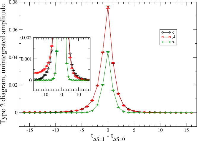
Figure 4: Unintegrated scalar amplitude for the Type 2 diagram.

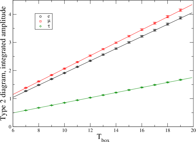
Figure 5: Integrated scalar amplitude for the Type 2 diagram. The unphysical exponentially growing terms for the muon have been subtracted.

In contrast to the Type 1 diagram, even after the GIM subtraction, the Type 2 diagram contains a logarithmic SD (ultraviolet) divergence which needs to be removed as explained in detail in Sec. IV. The unintegrated scalar amplitude is shown in Fig. 4 as a function of $t_{\Delta S=1}-t_{\Delta S=0}$. By zooming into the plots, we can observe the exponentially growing time dependence for the muon. This exponential behavior is not very significant however, since now the intermediate ground state is $|\pi^{0}\ell^{+}\nu\rangle$ and its energy is similar to $m_{K}$. Nevertheless this unphysical term still contributes a sizeable systematic effect and needs to be subtracted. We therefore calculate the matrix elements $\langle\pi^{+}\nu\bar{\nu}|O_{u\ell}^{\Delta S=0}(0)|\pi^{0}\ell^{+}\nu\rangle$ and $\langle\pi^{0}\ell^{+}\nu|O_{u\ell}^{\Delta S=1}(0)|K^{+}\rangle$ to remove this unphysical term. For the Type 2 diagram, we do not observe the exponentially growing behavior for the electron. In general we would expect there to be no helicity suppression in this case, since the intermediate ground state is now semi-leptonic, rather than the leptonic one for the Type I diagram. In our calculation, we use the discrete lattice momenta $-(2\pi/L){\bf n}$ for the intermediate hadronic particles and momenta ${\bf p}_{K}-{\bf p}_{\nu}+(2\pi/L){\bf n}$ for the intermediate lepton $\ell^{+}$. With such assignments, in the intermediate ground state, the neutral pion carries zero momentum and the helicity suppression still holds for the electron. This is the reason why we don’t observe an exponentially growing term for the electron. The assignment of the spatial momenta for the intermediate-state particles is clearly not unique. Different assignments will introduce different finite-size effects Christ et al. (2015b) and we will discuss this topic later.

The integrated scalar amplitude for the Type 2 diagram is shown in Fig. 5. After removing the exponential unphysical contributions and fitting the lattice data to a linear function of $T_{\mathrm{box}}$, we determine the values of $F_{WW}$ and include them in Table 3. We also compute the contributions from the lowest $|\pi^{0}\ell^{+}\nu\rangle$ intermediate state and compare them with the total result for the Type 2 diagram. For the muon the contribution from $|\pi^{0}\mu^{+}\nu\rangle$ is only 16% of the total contribution. Significant contributions come from the excited states, suggesting that the amplitude for Type 2 diagram contains a large SD contribution. This SD contribution is cut off by the unphysical lattice scale $1/a$. We must introduce a counter term to obtain the physical amplitude, as explained in Sec. IV below.

III.6 The matrix element of the bilocal operator for the $Z$-exchange diagrams

Examples of $Z$-exchange diagrams are given in Fig. 2. We write the bilocal matrix element in the form

$$T_{Z}({\bf p}_{K},{\bf p}_{\pi}) = \int d^{4}x\,\langle\pi^{+}\nu\bar{\nu}|T[O_{u}^{W}(x)O_{\ell}^{Z}(0)]|K^{+}\rangle-\{u\to c\}$$ (46)

$$= T^{Z}_{\mu}({\bf p}_{K},{\bf p}_{\pi})\left[\bar{u}(p_{\nu})\gamma_{\mu}(1-\gamma_{5})v(p_{\bar{\nu}})\right],$$

where $O_{q}^{W}$ and $O_{\ell}^{Z}$ are defined in Eq. (19). The hadronic part of $T_{Z}$ is given by

$$T^{Z}_{\mu}({\bf p}_{K},{\bf p}_{\pi})=\int d^{4}x\,\langle\pi^{+}|T[O_{u}^{W}(x)J_{\mu}^{Z}(0)]|K^{+}\rangle-\{u\to c\}.$$ (47)

We separate $T^{Z}_{\mu}$ into two parts: $T^{Z}_{\mu}=T^{Z,V}_{\mu}+T^{Z,A}_{\mu}$, corresponding to the vector ($V$) and axial vector ($A$) components of $J_{\mu}^{Z}$. The $K\to\pi Z^{*}$ form factors are conventionally defined by

$$T_{\mu}^{Z,i}({\bf p}_{K},{\bf p}_{\pi})=i\,\left(F_{+}^{Z,i}(s)(p_{K}+p_{\pi})_{\mu}+F_{-}^{Z,i}(s)(p_{K}-p_{\pi})_{\mu}\right),\quad i=V,A,$$ (48)

where $s=-(p_{K}-p_{\pi})^{2}$.

Since the spinor product $\bar{u}(p_{\nu}){\not{q}}(1-\gamma_{5})v(p_{\bar{\nu}})$ vanishes for massless neutrinos, only the form factors $F_{+}^{Z,i}(q^{2})$ contribute to the decay amplitude. For the vector current, the Ward-Takahashi identity guarantees

$$(m_{K}^{2}-m_{\pi}^{2})F_{+}^{Z,V}(s)=-sF_{-}^{Z,V}(s).$$ (49)

For the axial vector current, in order to determine $F_{+}^{Z,A}(s)$ from $T_{\mu}^{Z,A}({\bf p}_{K},{\bf p}_{\pi})$, we need to compute the amplitude $T_{\mu}^{Z,A}({\bf p}_{K},{\bf p}_{\pi})$ for different choices of the polarization $\mu$. This requires that either the kaon in the initial state or the pion in the final state (or both) carries a non-zero spatial momentum.

Although we cannot determine $F_{+}^{Z,i}(s)$ directly from $T_{\mu}^{Z,i}({\bf 0},{\bf 0})$, where both kaon and pion are at rest, we still calculate such matrix element for two reasons. Firstly, in our calculation we have used the local vector current rather than the conserved vector current. Due to the violation of the Ward-Takahashi identity, there will be a SD singularity when the operator $J_{\mu}^{Z,V}$ approaches the operator $O_{q}^{W}$. This SD contribution is independent of the kaon and pion momenta ${\bf p}_{K}$ and ${\bf p}_{\pi}$. As a result, we can use $T_{\mu}^{Z,V}({\bf 0},{\bf 0})$ to remove the SD divergence in $T_{\mu}^{Z,V}({\bf p}_{K},{\bf p}_{\pi})$. Secondly, for the insertion of the axial vector current ($i=A$), the matrix element $T_{\mu}^{Z,A}({\bf 0},{\bf 0})$ provides the most accurate data we can obtain for the $Z$-exchange diagrams. We define the scalar function $F_{0}^{Z,A}(s)$ by

$$F_{0}^{Z,A}(s)\equiv F_{+}^{Z,A}(s)+\frac{s}{m_{K}^{2}-m_{\pi}^{2}}F_{-}^{Z,A}(s).$$ (50)

At ${\bf p}_{K}=0$ and ${\bf p}_{\pi}=0$, we obtain from $T_{\mu}^{Z,A}({\bf 0},{\bf 0})$ the scalar function of $F_{0}^{Z,A}(s_{\mathrm{max}})$, where the variable $s$ takes its maximal value of $s_{\mathrm{max}}=(m_{K}-m_{\pi})^{2}$. As we will argue later, $F_{0}^{Z,A}(s_{\mathrm{max}})$ gives a good approximation to $F_{+}^{Z,i}(s)$ at $s=0$ (for the momentum choice in Eq. (13)).

III.6.1 Quark loops and disconnected diagrams

The operators $O_{q}^{W}$ defined in Eq. (19) can induce closed quark loops through the contraction of $u$ and $c$-quark loops. Given each gauge configuration, the $N_{r}$ components of the random volume-source light and charm quark propagators, which have already been used for the 3-point correlator, can also be used for the 4-point correlator. In addition, in order to be able to evaluate the disconnected diagrams in which $\pi\,O_{q}^{W}\,K$ and $J_{\mu}^{Z}$ form two separate loops, we have also calculated 32 random volume-source propagators for the strange quark. Thus we can perform a full calculation, which includes all connected, self-loop and disconnected diagrams.

III.6.2 Using chiral ward identities to remove the unphysical terms

For the $Z$-exchange diagrams, we start by inserting a complete set of intermediate states between the operators $O_{u}^{W}$ and $J_{\mu}^{Z}$ in Eq. (47). In order to obtain the physical result we need to remove the exponentially growing terms arising from the intermediate states whose energies are smaller than the mass of the initial kaon. For the vector current component of $J_{\mu}^{Z}$, the odd-parity intermediate states $|\pi^{+}\rangle$ and $|3\pi\rangle$ contain exponentially growing contributions Christ et al. (2015a). The exponentially growing contribution from the three-pion state can safely be neglected because of phase space suppression (and in the present calculation it is absent since $m_{K}<3m_{\pi}$). The unphysical contribution from the single-pion state can be removed by adding to the weak Hamiltonian $H_{W}=O_{u}^{W}-O_{c}^{W}$ a term proportional to the scalar density: $H_{W}^{\prime}=H_{W}-c_{s}\,\bar{s}d$. The chiral Ward identities imply that the addition of the term proportional to the scalar density does not change the on-shell matrix element Christ et al. (2013); Bai et al. (2014); Christ et al. (2015a). The coefficient $c_{s}$ can be determined by requiring that

$$\langle\pi^{+}({\bf 0})|H_{W}(0)-c_{s}\,\bar{s}d(0)|K^{+}({\bf 0})\rangle=0.$$ (51)

and our lattice results for $c_{s}$ are listed in Table 2.

For the axial-vector current component of $J_{\mu}^{Z}$, the parity-even state $|2\pi\rangle$ can produce an exponentially growing unphysical term. In this case it is not possible to add a term proportional to the pseudoscalar density ($H_{W}\to H_{W}^{\prime}=H_{W}-c_{p}\,\bar{s}\gamma_{5}d$) in such a way as to remove the $I=2$ two-pion contribution. This is because the combination of initial $K^{+}$ state and the pseudoscalar density $\bar{s}\gamma_{5}d$ cannot create an $I=2$ $\pi\pi$ state. Instead, as shown in Table 2, we have explicitly calculated the matrix elements $\langle(\pi^{+}\pi^{0})_{I=2}({\bf 0})|Q_{i,q}|K^{+}({\bf 0})\rangle$ and $\langle\pi^{+}({\bf 0})|\bar{u}\gamma_{t}\gamma_{5}u-\bar{d}\gamma_{t}\gamma_{5}d|(\pi^{+}\pi^{0})_{I=2}({\bf 0})\rangle$ and are therefore able to remove the unphysical term from the $|2\pi\rangle$ intermediate state (if it exists). For the current lattice calculation, since $m_{K}<2m_{\pi}$, no removal of such an unphysical term is required. Nevertheless the evaluation of these matrix elements of local operators allows us to determine the contribution to the $Z$-exchange diagrams from the $\pi\pi$ intermediate ground state in preparation for future simulations at physical light-quark masses.

III.6.3 The local vector current and the short-distance divergence

If one uses the conserved vector current, then gauge invariance implies that one can write $T_{\mu}^{Z,V}({\bf p}_{K},{\bf p}_{\pi})$ as

$$T_{\mu}^{Z,V}({\bf p}_{K},{\bf p}_{\pi})=i\left(-\frac{s}{m_{K}^{2}-m_{\pi}^{2}}(p_{K}+p_{\pi})_{\mu}+(p_{K}-p_{\pi})_{\mu}\right)F_{-}^{Z,V}(s).$$ (52)

The simplest choice of momenta for the $K\to\pi Z^{*}$ transition is ${\bf p}_{K}={\bf p}_{\pi}={\bf 0}$, where ${\bf p}_{K}$ and ${\bf p}_{\pi}$ are the spatial momenta of the kaon in the initial state and the pion in the final state. Such a choice of momenta is not very useful however, since the kinematic factor $-\frac{s}{m_{K}^{2}-m_{\pi}^{2}}(p_{K}+p_{\pi})_{\mu}+(p_{K}-p_{\pi})_{\mu}$ is then equal to $0$. As a consequence, the transition amplitude $T_{\mu}^{Z,V}({\bf 0},{\bf 0})$ vanishes. However, by using the local vector current instead of the conserved one, this simple choice of momenta proves to be useful in making a SD correction as we now explain.

With the local vector current we can no longer use the Ward-Takahashi identity to obtain (52). The operator product expansion of $Q_{i,q}(x)J_{\mu}^{V_{\textrm{loc}}}(0)$ can be written in the form

$$Q_{i,q}(x)J_{\mu}^{V_{\textrm{loc}}}(0)\simeq c_{1}\bar{s}\gamma_{\mu}^{L}d+c_{2}\bar{s}\gamma_{\nu}^{L}(\partial^{2}\delta_{\mu\nu}-\partial_{\mu}\partial_{\nu})d+c_{3}\bar{s}\gamma_{\nu}^{L}\partial_{\mu}\partial_{\nu}d+\cdots$$ (53)

where $\gamma_{\mu}^{L}\equiv\gamma_{\mu}(1-\gamma_{5})$ and for compactness of notation we have suppressed the label $i$ on the right-hand side. Dimensional analysis shows that the coefficient $c_{1}\sim 1/x^{6}$ at small distances, leading to a $1/a^{2}$ quadratic divergence after integration over $x$, while $c_{2}$ and $c_{3}$ both $\sim 1/x^{4}$ corresponding to a $\log a^{2}$ logarithmic divergence. All the higher-dimension terms are accounted for by the ellipsis in Eq. (53). It is the $c_{2}$-term which is physical and the terms with coefficients $c_{1}$ and $c_{3}$ appear because of the use of the local vector current. By applying the GIM mechanism, i.e. subtracting the charm quark contribution ($i=c$) from that of the up quark ($i=u$) we reduce the divergence in the integrated correlation function from the term proportional to $c_{1}$ to a logarithmic one and remove the divergences from the terms proportional to $c_{2,3}$, leaving them finite. The logarithmic divergence in the term proportional to $c_{1}$ arises from the contact term as $x$ approaches $0$ in $Q_{i,q}(x)J_{\mu}^{V_{\textrm{loc}}}(0)$. In order to subtract this divergence we introduce a counter term $X_{V}\,\bar{s}\gamma_{\mu}^{L}d$ writing

$$T_{\mu}^{Z,V}({\bf p}_{K},{\bf p}_{\pi})=Z_{V}\left(T_{\mu}^{Z,V_{\textrm{loc}}}({\bf p}_{K},{\bf p}_{\pi})-X_{V}\,\langle\pi^{+}({\bf p}_{\pi})|\bar{s}\gamma_{\mu}^{L}d(0)|K^{+}({\bf p}_{K}\rangle\right)\,,$$ (54)

where

$$T_{\mu}^{Z,V_{\textrm{loc}}}({\bf p}_{K},{\bf p}_{\pi})=\int d^{4}x\,\langle\pi^{+}({\bf p}_{\pi})|T[O_{u}^{W}(x)J_{\mu}^{V_{\textrm{loc}}}(0)]|K^{+}({\bf p}_{K})\rangle-\{u\to c\},$$ (55)

and the superscript $V_{\textrm{loc}}$ indicates the insertion of the local vector current. A natural condition which can be used to define and determine the coefficient $X_{V}$ is $T_{\mu}^{Z,V}({\bf 0},{\bf 0})=0$, i.e.

$$T_{\mu}^{Z,V_{\textrm{loc}}}({\bf 0},{\bf 0})-X_{V}\,\langle\pi^{+}({\bf 0})|\bar{s}\gamma_{\mu}d(0)|K^{+}({\bf 0})\rangle=0.$$ (56)

Once $X_{V}$ is determined, we obtain the form factor $F_{+}^{Z,V}(s)$ for the choice of momenta in (13) with the contact term removed using

$$F_{+}^{Z,V}(s)=F_{+}^{Z,V_{\textrm{loc}}}(s)-X_{V}\,f_{+}(s),$$ (57)

where $F_{+}^{Z,V_{\textrm{loc}}}(s)$ is obtained from

$$Z_{V}T_{\mu}^{Z,V_{\textrm{loc}}}({\bf p}_{K},{\bf p}_{\pi})=i\,\left(F_{+}^{Z,V_{\textrm{loc}}}(s)(p_{K}+p_{\pi})_{\mu}+F_{-}^{Z,V_{\textrm{loc}}}(s)(p_{K}-p_{\pi})_{\mu}\right)$$ (58)

and $f_{+}(s)$ is defined in Eq. (23). For the particular choice of momenta given in Eq. (13) $s=0$ and the Ward-Takahashi identity (49) implies that $F_{+}^{Z,V}(s)=0$ at $s=0$. We will show later that our lattice result for $F_{+}^{Z,V}(s)$ is indeed consistent with $0$ within the statistical errors. For other values of $s$, $F_{+}^{Z,V}(s)$ does not vanish and the procedure described in this section allows for its determination.

Note that the term proportional to $c_{3}$ vanishes in the continuum limit. Having used the GIM mechanism to reduce the degree of divergence and subtracted the remaining contact term by introducing the counterterm, we can relate the conserved and local vector currents ($J_{\mu}^{V_{\textrm{con}}}$ and $J_{\mu}^{V_{\textrm{loc}}}$ respectively) by $J_{\mu}^{V_{\textrm{con}}}=Z_{V}J_{\mu}^{V_{\textrm{loc}}}$ up to lattice artifacts. Since the artifacts vanish in the continuum limit, so does $c_{3}$.

III.6.4 Single integration method

As explained in Sec. III.5.5, when calculating the matrix element for the $W$-$W$ diagrams we have used the double integration method. At large $T_{\mathrm{box}}$ the method requires the lattice data to be fit using a simple linear function. However, the drawback of this method is that the lattice data for small separations $t_{2}-t_{1}$ of the two weak operators are included only when the source-sink separation $t_{\pi}-t_{K}\gg T_{\mathrm{box}}$. In fact, this data will accurately contribute to the bilocal matrix element provided $t_{\pi}-t_{K}\gg|t_{2}-t_{1}|$. The smaller values of $t_{\pi}-t_{K}$ allowed by this less stringent condition will give data with smaller errors. The single integration method described in this section makes use of this more accurate data, and are able to significantly improve the precision for the $Z$-exchange diagrams. For the $W$-$W$ diagrams the lepton in the intermediate state is not affected by the gauge noise and there would be no improvement.

For the $Z$-exchange diagrams we adopt the single integration method. Given the time locations of the kaon and pion interpolating operators, $t_{K}$ and $t_{\pi}$ respectively, we determine the unintegrated matrix element using

$$T_{\mu}^{Z,i}(t_{\pi},t_{H},t_{J},t_{K})=\frac{4E_{\pi}E_{K}}{N_{\pi}N_{K}}\langle\phi_{\pi}(t_{\pi})O_{q}^{W}(t_{H})J_{\mu}^{Z,i}(t_{J})\phi^{\dagger}_{K}(t_{K})\rangle e^{E_{\pi}(t_{\pi}-t_{J})}e^{E_{K}(t_{J}-t_{K})}\,.$$ (59)

By examining the numerical results for $T_{\mu}^{Z,i}(t_{\pi},t_{H},t_{J},t_{K})$ as functions of $t_{H}$ and $t_{J}$, we conclude that for $t_{\pi}-t_{H,J}\geq 6$ and $t_{H,J}-t_{K}\geq 6$, the effects from excited states can be safely neglected (this is consistent with the corresponding observations for the $W$-$W$ diagrams). For such time separations, by using time-translation invariance $T_{\mu}^{Z,i}(t_{\pi},t_{H},t_{J},t_{K})$ only depends on the time difference between $t_{H}$ and $t_{J}$. For fixed time separations $t=t_{H}-t_{J}$ (but different locations of $t_{J}$) we fit the matrix elements $T_{\mu}^{Z,i}(t_{\pi},t_{H},t_{J},t_{K})$ to a constant and obtain the average value $\bar{T}_{\mu}^{Z,i}(t_{\pi},t,t_{K})$. We then use these results for $\bar{T}_{\mu}^{Z,i}(t_{\pi},t,t_{K})$, to perform a second fit, this time over $t_{\pi}$ and $t_{K}$ for each value of $t$. In this way, we obtain the matrix element $\bar{\bar{T}}_{\mu}^{Z,i}(t)$, which contains the information from all the lattice data constrained by $\{t_{\pi},t_{H},t_{J},t_{K}|\,t_{H}-t_{J}=t,t_{H,J}-t_{K}\geq 6,t_{\pi}-t_{H,J}\geq 6\}$. We then perform a single integration of $\bar{\bar{T}}_{\mu}^{Z,i}(t)$ over the variable $t$ in the range $-T_{\textrm{box}}\leq t\leq T_{\textrm{box}}$ and find the plateau for large $T_{\textrm{box}}$, once the unphysical terms growing exponentially with $T_{\textrm{box}}$ have been removed. Since all the possible data for $t_{H}-t_{J}=t$ have been used, the single integration method decreases the statistical error for the $Z$-exchange diagrams by 30%-40% when compared to the double integration method.

III.6.5 Lattice results

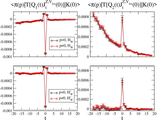
Figure 6: The unintegrated matrix elements for the $Z$-exchange diagrams with the vector current component of $J_{\mu}^{Z}$. The vector current polarization direction is chosen to be $\mu=t$. In the upper panel, the matrix elements $\int d^{3}\vec{x}\,\langle\pi^{+}(p_{\pi})|T[H_{W}(\vec{x},t)J_{\mu=t}^{V_{\textrm{loc}}}(0)|K^{+}(0)\rangle$ (for the $Q_{1,q}$ and $Q_{2,q}$ components) are shown as functions of $t=t_{H}-t_{J}$. The black circle data points show the lattice results for the momentum mode ${\bf p}_{K}={\bf p}_{\pi}={\bf 0}$; the red square points show the results for ${\bf p}_{K}={\bf 0}$ and with ${\bf p}_{\pi}\neq{\bf 0}$ and taking the value in Eq. (13). The exponentially growing time dependence can be seen at $t\ll 0$. In the lower panel, the matrix elements are calculated using the modified Hamiltonian $H_{W}^{\prime}=H_{W}-c_{s}\,\bar{s}d$, so that the exponentially growing terms have been removed.

We start by presenting the numerical results for the vector current component of $J_{\mu}^{Z}$. The unintegrated matrix elements $\bar{\bar{T}}_{\mu}^{Z,V_{\textrm{loc}}}(t)$ as a function of the time separation $t=t_{H}-t_{J}$ are shown in the upper panel of Fig. 6. Since the four-fermion operator $O_{q}^{W}$ is a linear combination of $Q_{1,q}$ and $Q_{2,q}$, we show the numerical results for each operator. When the polarization index of the vector current $J_{\mu}^{V_{\textrm{loc}}}$ is a spacial one, i.e. when $\mu=i=x,\,y$ or $z$, the matrix element is supressed by a factor of ${\bf p}_{\pi,i}/m_{K}$ as shown in Eq. (52). For this reason and in order to facilitate the comparison of the matrix element at zero and non-zero ${\bf p}_{\pi}$ we plot the matrix element with $\mu=t$. The black circle data points show the lattice results for the momentum ${\bf p}_{K}={\bf p}_{\pi}={\bf 0}$; the red square points show the results for ${\bf p}_{K}={\bf 0}$ and with ${\bf p}_{\pi}$ taking the non-zero value given in Eq. (13). As ${\bf p}_{\pi}$ is small, it is not surprising that the black circle and red square data points are very close to each other.

In the time region $t\ll 0$, the dominant intermediate state is the $|\pi^{+}\rangle$. Since this state is lighter than the initial kaon there is an exponentially growing contribution as shown in the upper panel of Fig. 6. We remove this unphysical contribution by adding to the weak Hamiltonian a term proportional to the scalar density $c_{s}\,\bar{s}d$, with the value of $c_{s}$ given in Table 2 and show in the lower panel of Fig. 6 that after correction the lattice data does indeed converge to a constant at $t\ll 0$.

For both the vector and axial-vector components of the weak current $J_{\mu}^{Z}$ we have only calculated the contribution of the disconnected diagrams with ${\bf p}_{K}={\bf p}_{\pi}={\bf 0}$. For the vector current, the Ward identity implies that the amplitude is zero in this case (i.e. the numerical results are simply gauge noise) and so we do not include the contribution from the disconnected diagrams in Fig. 6. For the axial current the amplitude does not vanish for ${\bf p}_{K}={\bf p}_{\pi}={\bf 0}$ and below we do include the contribution from the disconnected diagrams in Fig. 7 and the corresponding text.

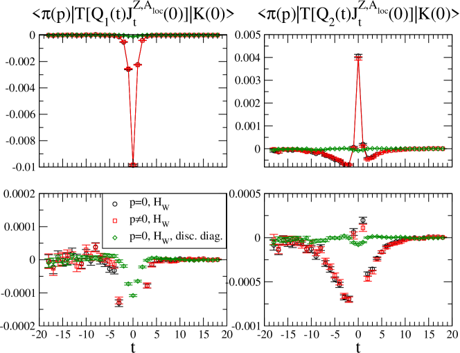
Figure 7: Unintegrated matrix elements for the $Z$-exchange diagrams with the axial vector current component. The axial vector current polarization direction is chosen to be $\mu=t$. At $m_{\pi}=420$ MeV, no exponentially growing term is observed at $t\ll 0$. The black circle data points show the lattice results for the momentum ${\bf p}_{K}={\bf p}_{\pi}={\bf 0}$; the red square points show the results for ${\bf p}_{K}={\bf 0}$ and with ${\bf p}_{\pi}\neq{\bf 0}$ and taking the value in Eq. (13). These results include only the connected and self-loop diagrams. For the disconnected diagrams, the corresponding results are shown by the green diamond symbol. Although noisy, the disconnected contributions are much smaller than the connected ones.

For the axial-vector current component of $J_{\mu}^{Z}$ it is not possible to use the (partially) conserved current to avoid having to make a subtraction of the short-distance divergence, as was done for the vector current in Sec. III.6.3. We therefore use the local axial-vector current and follow the general procedure for the subtraction of the SD divergence using the RI/SMOM intermediate scheme, as explained in detail in Sec. IV. The unintegrated matrix elements are shown in Fig. 7. At $t\ll 0$ the time dependence is dominated by the two-pion state, whose energy $E_{\pi\pi}\approx 2m_{\pi}$ with, in this simulation, $m_{\pi}=420$ MeV which is larger than the initial kaon mass. Thus we do not observe the exponentially growing $t$ dependence.

In addition to the connected diagrams in Fig. 2, we also calculate the disconnected diagrams and produce results including all quark contractions. The summation of up, down and strange quark loops vanish in the flavor $SU(3)$ limit. The remaining charm quark loop is suppressed due to the heavy charm quark mass. So we expect that the absolute size of the disconnected diagrams is small. This expectation is confirmed by a comparison between disconnected data points (the green diamond symbol in Fig. 7) and the connected and self-loop ones (the black circle symbol). Due their small size, although the disconnected diagrams have much larger relative statistical errors, they do not contribute a large uncertainty in the total decay amplitude. Thus a complete lattice QCD calculation including all the diagrams is practical.

The lattice results for the matrix elements of the bilocal operators from the $Z$-exchange diagrams are summarized in Table 4. The lattice data are shown in three columns for the $Q_{1,q}^{\mathrm{lat}}$ and $Q_{2,q}^{\mathrm{lat}}$ operators and also for the combination $C_{1}^{\mathrm{lat}}Q_{1,q}+C_{2}^{\mathrm{lat}}Q_{2,q}$. Here $C_{1}^{\mathrm{lat}}=-0.2186$ and $C_{2}^{\mathrm{lat}}=0.6424$ are Wilson coefficients in the lattice regularization. They can be related to the Wilson coefficients in the $\overline{\mathrm{MS}}$ scheme by a $2\times 2$ conversion matrix $Z^{\mathrm{lat}\to\overline{\mathrm{MS}}}$. The details will be discussed in Sec. IV. In Table 4, starting at the top we first show the matrix elements for the $K^{+}({\bf 0})\to\pi^{+}(\bf{0})$ transition. For the vector-current component, these matrix elements can be used to determine the coefficient $X_{V}$ of the counter-term and to correct the SD divergence for the $Q_{i,q}(x)J_{\mu}^{Z,V_{\textrm{loc}}}(0)$ bilocal operator. For the axial vector-current component, we can use these matrix elements to determine $F_{0}^{Z,A}(s_{\mathrm{max}})$. The calculation of $F_{0}^{Z,A}(s_{\mathrm{max}})$ proves to be useful for our exploratory study as it provides approximate information about $F_{+}^{Z,A}(s_{\mathrm{max}})$, see Eq. (50). For the $K^{+}({\bf 0})\to\pi^{+}({\bf 0})$ transition, we also include the contributions from the disconnected diagrams in the calculation of $F_{0}^{Z,A}(s_{\mathrm{max}})$; these data are labeled by the subscript disc. This is not currently possible for the direct evaluation of $F_{+}^{Z,A,disc}(0)$, for which we need to use twisted boundary conditions. Next in Table 4 we show the matrix elements for the $K^{+}({\bf 0})\to\pi^{+}({\bf p})$ transition, where the spatial momentum of the pion is given by Eq. (13). Due to the non-zero momentum of the pion, we are able to obtain the scalar function $F_{+}^{Z,i}(0)$ from these data. From Table 4 we obtain the following information.

• The contribution from the vector current $F_{+}^{Z,V}(s)$ (which is proportional to $s$) is expected to be much smaller than that from the axial vector current $F_{+}^{Z,A}(s)$ (which is proportional to $m_{c}^{2}$). This is confirmed by our lattice data.

• At the special momentum transfer $s=0$ we expect that $F_{+}^{Z,V}(0)=0$ because of the Ward-Takahashi identity (49). This holds for the conserved vector current or, as in the present case, by using the local vector current and subtracting the SD counterterm. We see from the table that after subtracting the counter-term, $F_{+}^{Z,V_{\textrm{loc}}}(0)-X_{V}f_{+}(0)$ is consistent with zero within 1$\sigma$. We also see that $F_{+}^{Z,V_{\textrm{loc}}}(0)$ itself is significantly different from 0.

• For the axial vector current, we observe that $F_{0}^{Z,A}(s_{\mathrm{max}})\approx F_{0}^{Z,A}(0)=F_{+}^{Z,A}(0)$. Although we are interested in $F_{+}^{Z,A}(s)$, we conclude that the lattice determination of $F_{0}^{Z,A}(s)$ can be used as a good approximation for $F_{+}^{Z,A}(s)$ for small values of $s$ since $F_{-}^{Z,A}(s)$ is much smaller than $F_{+}^{Z,A}(s)$.

• The disconnected diagrams have been evaluated for the transition $K^{+}({\bf 0})\to\pi^{+}({\bf 0})$. The contribution from these diagrams $F_{0}^{Z,A,disc}(s_{\mathrm{max}})$ is about 3% of that from the connected diagrams $F_{0}^{Z,A}(s_{\mathrm{max}})$. If we accept that $F_{0}^{Z,A}(s)$ approximates $F_{+}^{Z,A}(s)$, then the disconnected diagrams only make a small contribution to the $Z$-exchange diagrams.

$Z$-exchange diagrams
$K^{+}({\bf 0})\to\pi^{+}({\bf 0})$	$Q_{1}$	$Q_{2}$	$C_{1}^{\mathrm{lat}}Q_{1}+C_{2}^{\mathrm{lat}}Q_{2}$
$\langle\pi^{+}({\bf 0})|H_{W}\,J_{t}^{V_{\textrm{loc}}}|K^{+}({\bf 0})\rangle_{conn}$	$31.5(1.8)\cdot 10^{-4}$	$13.5(2.0)\cdot 10^{-4}$	$1.8(1.5)\cdot 10^{-4}$
$X_{V}$ defined by Eq. (56)	$-39.4(2.2)\cdot 10^{-4}$	$-16.9(2.5)\cdot 10^{-4}$	$-2.2(1.9)\cdot 10^{-4}$
$\langle\pi^{+}({\bf 0})|H_{W}\,J_{t}^{A_{\textrm{loc}}}|K^{+}({\bf 0})\rangle_{conn}$	$7.313(41)\cdot 10^{-2}$	$-0.121(22)\cdot 10^{-2}$	$-1.676(19)\cdot 10^{-2}$
$F_{0}^{Z,A}(s_{\mathrm{max}})$	$-9.202(61)\cdot 10^{-2}$	$0.152(28)\cdot 10^{-2}$	$2.109(25)\cdot 10^{-2}$
$\langle\pi^{+}({\bf 0})|H_{W}\,J_{t}^{A_{\textrm{loc}}}|K^{+}({\bf 0})\rangle_{disc}$	$11.1(1.3)\cdot 10^{-4}$	$-3.7(1.1)\cdot 10^{-4}$	$-4.8(0.9)\cdot 10^{-4}$
$F_{0}^{Z,A,disc}(s_{\mathrm{max}})$	$-13.9(1.7)\cdot 10^{-4}$	$4.7(1.4)\cdot 10^{-4}$	$6.0(1.2)\cdot 10^{-4}$
$K^{+}({\bf 0})\to\pi^{+}({\bf p_{\pi}})$
$\langle\pi^{+}({\bf p_{\pi}})|H_{W}\,J_{t}^{V_{\textrm{loc}}}|K^{+}({\bf 0})\rangle_{conn}$	$27.9(1.8)\cdot 10^{-4}$	$15.0(2.0)\cdot 10^{-4}$	$3.5(1.6)\cdot 10^{-4}$
$\langle\pi^{+}({\bf p_{\pi}})|H_{W}\,J_{i}^{V_{\textrm{loc}}}|K^{+}({\bf 0})\rangle_{conn}$	$i\cdot 3.4(0.8)\cdot 10^{-4}$	$i\cdot 1.5(0.8)\cdot 10^{-4}$	$i\cdot 0.2(0.7)\cdot 10^{-4}$
$F_{+}^{Z,V_{\textrm{loc}}}(0)$	$-37.3(2.5)\cdot 10^{-4}$	$-19.1(2.7)\cdot 10^{-4}$	$-4.1(2.1)\cdot 10^{-4}$
$F_{+}^{Z,V_{\textrm{loc}}}(0)-X_{V}f_{+}(0)$	$-1.8(1.7)\cdot 10^{-4}$	$-2.4(1.8)\cdot 10^{-4}$	$-1.9(1.4)\cdot 10^{-4}$
$\langle\pi^{+}({\bf p_{\pi}})|H_{W}\,J_{t}^{A_{\textrm{loc}}}|K^{+}({\bf 0})\rangle_{conn}$	$7.276(44)\cdot 10^{-2}$	$-0.141(24)\cdot 10^{-2}$	$-1.681(20)\cdot 10^{-2}$
$\langle\pi^{+}({\bf p_{\pi}})|H_{W}\,J_{i}^{A_{\textrm{loc}}}|K^{+}({\bf 0})\rangle_{conn}$	$i\cdot 0.600(17)\cdot 10^{-2}$	$-i\cdot 0.026(16)\cdot 10^{-2}$	$-i\cdot 0.148(12)\cdot 10^{-2}$
$F_{+}^{Z,A_{\textrm{loc}}}(0)=F_{0}^{Z,A_{\textrm{loc}}}(0)$	$-9.158(64)\cdot 10^{-2}$	$0.204(41)\cdot 10^{-2}$	$2.133(32)\cdot 10^{-2}$
$F_{-}^{Z,A_{\textrm{loc}}}(0)$	$1.22(27)\cdot 10^{-2}$	$-0.24(24)\cdot 10^{-2}$	$-0.42(18)\cdot 10^{-2}$

Table 4: Summary of the matrix elements of the bilocal operators and the form factors for the $Z$-exchange diagrams. The momentum transfer $s$ is given by $s=s_{\mathrm{max}}=(m_{K}-m_{\pi})^{2}$ for the $K^{+}({\bf 0})\to\pi^{+}({\bf 0})$ transition and $s=0$ for the $K^{+}({\bf 0})\to\pi^{+}({\bf p_{\pi}})$ with ${\bf p_{\pi}}$ given in Eq. (13).

We end this section by estimating the contribution from the lowest energy $|(\pi\pi)_{I=2}\rangle$ state to the $Z$-exchange diagrams. Using the computed matrix elements $A_{\pi\pi\to\pi}\equiv\langle\pi^{+}(0)|\bar{u}\gamma_{t}\gamma_{5}u-\bar{d}\gamma_{t}\gamma_{5}d|(\pi^{+}\pi^{0})_{I=2}(0)\rangle$ and $A_{K\to\pi\pi}\equiv\langle(\pi^{+}\pi^{0})_{I=2}(0)|Q_{i,q}|K^{+}(0)\rangle$ given in Table 2 we construct the $\pi\pi$ contribution as

$$T_{\mu=t}^{Z,A,\pi\pi}(s_{\mathrm{max}})=Z_{A}(-T_{3}^{u})A_{\pi\pi\to\pi}\frac{1}{2E_{\pi\pi}}\frac{1}{E_{\pi\pi}-m_{K}}(C_{1}^{\mathrm{lat}}+C_{2}^{\mathrm{lat}})A_{K\to\pi\pi}\,,$$ (60)

where $Z_{A}=Z_{V}$ is the (axial) vector current renormalization factor and $T_{3}^{u}=\frac{1}{2}$ is the weak isospin associated with the axial vector current. The minus sign corresponds to that in the $V-A$ structure of the weak Hamiltonian. We finally determine the $\pi\pi$ contribution to the form factor using $F_{0}^{Z,A,\pi\pi}(s_{\mathrm{max}})=T_{\mu=t}^{Z,A,\pi\pi}(s_{\mathrm{max}})/(-(m_{K}+m_{\pi}))=1.526(10)\cdot 10^{-3}$, which is only 7% of the $F_{0}^{Z,A}(s_{\mathrm{max}})$ given in Table 4, suggesting that the dominant contribution to the $Z$-exchange diagrams comes from higher excited states and SD physics. Once simulations at physical quark masses are performed, when the two-pion state contributes exponentially growing contributions in $T_{\textrm{box}}$ which will need to be subtracted, its contribution to $F_{+}^{Z,A}$ will have to be studied again.

IV Removal of the short-distance divergence using nonperturbative renormalization

In this section we discuss the subtraction of the additional ultraviolet divergences which appear when the two local operators which are the components of a bilocal operator approach each other. In Sec. IV.1 we review the theoretical background and in Sec. IV.2 we present the numerical results for the subtraction constants.

IV.1 Non-perturbative renormalization using RI/SMOM scheme

In Sec. III.6.3, for the vector current insertion we have used the matrix element of the transition $K({\bf 0})\to\pi({\bf 0})$ to remove the SD divergence in the matrix element of the bilocal operators. Here we describe a more general method to remove the SD divergence, following the procedures developed in Ref. Christ et al. (2016a).

Given a bare lattice bilocal operator $\{Q_{A}^{\mathrm{lat}}Q_{B}^{\mathrm{lat}}\}^{\mathrm{lat}}_{a}$, in order to define and determine its SD component, we construct an off-shell Green’s function

$$G_{\alpha\beta\rho\sigma}^{AB}=\langle s_{\alpha}(p_{1})\nu_{\rho}(p_{3})\left[\int d^{4}x\,Q_{A}(x)Q_{B}(y)\right]\bar{d}_{\beta}(p_{2})\bar{\nu}_{\sigma}(p_{4})\rangle$$ (61)

where the fermionic fields $s$, $\bar{d}$, $\nu$ and $\bar{\nu}$ carry the non-exceptional Euclidean 4-momenta

$$p_{1}=(\xi,\xi,0,0),\quad p_{2}=(\xi,0,\xi,0),\quad p_{3}=(0,-\xi,0,-\xi),\quad p_{4}=(0,0,-\xi,-\xi).$$ (62)

The quark and lepton contractions contributing to the SD divergence are shown in Fig. 8. We choose the external momenta $p_{i}$ to satisfy $p_{i}^{2}\equiv\mu_{0}^{2}=2\xi^{2}$. The momentum $p_{\mathrm{loop}}$ flowing into the internal loop is given by $p_{\mathrm{loop}}=(\xi,0,0,-\xi)$ for $W$-$W$ diagrams and $p_{\mathrm{loop}}=(0,\xi,-\xi,0)$ for $Z$-exchange diagrams.

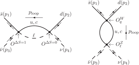
Figure 8: Left: SD divergent loop in $W$-$W$ diagrams. Right: SD divergent loop in $Z$-exchange diagrams.

For the $Z$-exchange diagrams the weak Hamiltonian is a linear combination of two operators $O_{1,q}$ and $O_{2,q}$ which mix under renormalization. The second operator however, is either the local vector or axial vector current with a multiplicative renormalization constant $Z_{V}$. For the $W$-$W$ diagrams both the operators $Q_{A}$ and $Q_{B}$, i.e. $Q_{q\ell}^{\Delta S=1}$ and $Q_{q\ell}^{\Delta S=0}$, renormalise multiplicatively. Nevertheless, in this section we present a general discussion in which both $Q_{A}$ and $Q_{B}$ mix with other operators and in the absence of such mixing the corresponding renormalization matrices in the formulae become numerical constants. In order to allow the RI/SMOM normalization to be imposed at four-momenta that can be held fixed in physical units in both magnitude and direction when we later perform a continuum extrapolation, we will use twisted external momenta whose components are nonecessarily integer multiples of $2\pi/L$ Arthur and Boyle (2011).

We perform the calculation in the Landau gauge. Imposing the twisted boundary condition on the quark field, $q(x+L\hat{\mu})=e^{i\theta_{\mu}}q(x)$, is equivalent to multiplying the gauge field by a factor of $e^{ip_{\mu}}$: $U_{\mu}\to U_{\mu}^{\prime}=e^{ip_{\mu}}U_{\mu}$, with $\theta_{\mu}=p_{\mu}L(\bmod 2\pi)$. We can consider this multiplication as a global $U(1)$ rotation. Since $p_{1}\neq p_{2}$, we multiply the gauge field by a different factor $e^{ip_{i,\mu}}$ when calculating the corresponding quark propagator. Calculating a zero-momentum volume-source quark propagator on the rotated gauge fields $U_{\mu}^{\prime}$ naturally assigns the non-zero external momentum $p_{i}$ for the external quark propagator. For the $Z$-exchange diagram, we rotate the gauge fields with a phase factor of $e^{ip_{{\mathrm{loop},\mu}}}$. Combining the point-source quark propagators with and without this gauge rotation, we can arrange that the internal loop can carry an appropriately twisted momentum $p_{\mathrm{loop}}$. For the $W$-$W$ diagram, the momentum $p_{\mathrm{loop}}$ is carried by the internal lepton field while the internal quark propagators are calculated with unrotated gauge fields. We treat the position $x$ of one operator as the source and the position $y$ of the other operator as the sink. The source $x$ is treated as a fixed, point source while the sink $y$ is summed over the full space-time volume after the other propagators connected to $y$ have been included. To improve the precision, we place the point source at $32$ different positions and then exploit translation-invariance to average over these source locations.

When implementing the non-perturbative renormalization as described above, we impose different (twisted) boundary conditions within the same diagram for different fermion propagators of the same flavor. We argue below that this can be done consistently for connected diagrams evaluated in the perturbative regime. This is in contrast to the use of different boundary conditions for different portions of an amplitude at low energies. For example, the effects of using different boundary condition for the valence and sea quarks require the study of an effective field theory and careful consideration of possible on-shell intermediate states Sachrajda and Villadoro (2005). Our use of multiple boundary conditions is introduced to allow specific external momenta and we now show that the errors introduced by this approach fall exponentially with the volume.

Because the usual RI/SMOM conditions are applied for large non-exceptional Euclidean external momenta, the amplitudes being studied are infrared safe and may be represented by a standard, all-orders perturbative sum. Further, we assume that the twist angles $\theta_{\mu}$ are rational multiples of $2\pi$, $\theta_{\mu}=2\pi(r_{\mu}/r)$ for five integers $r_{\mu}$, $0\leq\mu\leq 3$ and $r$. For a quark-line-connected diagram of the sort described above a sequence of twisted quark propagators is introduced connecting the vertex at which the twisted momentum enters to the vertex at which it exits so that momentum will be conserved at each vertex of the graph. If this same Green’s function were evaluated in a much larger volume of side $L^{\prime}=rL$, all of the momenta would be integral multiples of $2\pi/L^{\prime}$ with no twisting needed.

We now use the Poisson summation formula to argue that these two Green’s functions must differ by terms which vanish exponentially in the length $L$. In both cases we can use momentum conservation to route the twisted external momenta on the same path through the graph. The internal momentum sums for both volumes then involve momenta that are added to the twisted momentum, when present, carried by each quark line. For the original volume $L^{4}$, the result depends on the arbitrary routing of the twisted momentum. For the larger volume $(rL)^{4}$ the loop momenta can be redefined to move the path followed within the graph by the external momentum. Since there are no nearby singularities for such an off-shell Euclidean amplitude, the Poisson summation formula guarantees that these two sums over discrete internal momenta, one with $r^{4}$ more terms than the other, will differ by terms which vanish exponentially in the distance $L$ .

In the next step we calculate the amputated vertex $\Gamma_{\alpha\beta\rho\sigma}^{\mathrm{AB}}$ from the Green’s function through

$$\Gamma_{\alpha\beta\rho\sigma}^{\mathrm{AB}}=\langle S^{-1}_{s}(p_{1})\rangle_{\alpha\alpha^{\prime}}\langle S^{-1}_{d}(p_{2})\rangle_{\beta\beta^{\prime}}\langle S^{-1}_{\nu}(p_{3})\rangle_{\rho\rho^{\prime}}\langle S^{-1}_{\bar{\nu}}(p_{4})\rangle_{\sigma\sigma^{\prime}}G_{\alpha^{\prime}\beta^{\prime}\rho^{\prime}\sigma^{\prime}}^{\mathrm{AB}}$$ (63)

where $S^{-1}_{s,d}(p_{i})$ stand for the inverse of the full strange and down quark propagators and $S^{-1}_{\nu,\bar{\nu}}(p_{i})$ for the inverse of free neutrino propagators. Another amputated vertex $\Gamma^{0}_{\alpha\beta\rho\sigma}$ can be obtained from the Green’s function in Eq. (61) if the bilocal operator product $\int d^{4}x\,Q_{A}^{\mathrm{lat}}(x)Q_{B}^{\mathrm{lat}}(y)$ is replaced by a bare local operator $Q_{0}^{\mathrm{lat}}(y)$. At tree level, $\Gamma^{0}$ is simply given by $\hat{\Gamma}=[\gamma_{\mu}(1-\gamma_{5})]_{q}\otimes[\gamma_{\mu}(1-\gamma_{5})]_{\nu}$, where the subscript $q$ indicates the quark flavor space and $\nu$ the neutrino flavor space. The color structure is not shown explicitly in $[\gamma_{\mu}(1-\gamma_{5})]_{q}$ since at tree level it is trivial. We use $\hat{\Gamma}$ to construct the projector

$$\mathrm{P}=\frac{\hat{\Gamma}^{\dagger}}{\textmd{Tr}_{s,c}[\hat{\Gamma}^{\dagger}\hat{\Gamma}]}\,,$$ (64)

where $\textmd{Tr}_{s,c}$ requires the trace over both the spin and color indices. When the projector acts on $\hat{\Gamma}$ it yields $\mathrm{Tr}_{s,c}[\mathrm{P}\hat{\Gamma}]=1$.

We use the large external momenta $p_{i}^{2}=\mu_{0}^{2}\gg\Lambda_{\mathrm{QCD}}^{2}$ to capture the SD contribution to the bilocal operator product $\int d^{4}x\,Q_{A}^{\mathrm{lat}}(x)Q_{B}^{\mathrm{lat}}(y)$ and then relate this contribution to the projection of the amputated Green function $\Gamma_{0}$ of the local operator $Q_{0}^{\mathrm{lat}}(y)$, where with the same external momenta we require:

$$\textmd{Tr}_{s,c}[\mathrm{P}\Gamma^{\mathrm{AB}}]=X_{AB}^{\mathrm{lat}}(\mu_{0},a)\,\textmd{Tr}_{s,c}[\mathrm{P}\Gamma^{0}].$$ (65)

Recall that the local operator is $Q_{0}=(\bar{s}d)_{V-A}(\bar{\nu}\nu)_{V-A}$. Using the coefficient $X_{AB}^{\mathrm{lat}}(a,\mu_{0})$, we remove the SD divergence by constructing the subtraction $\int d^{4}x\,Q_{A}^{\mathrm{lat}}(x)Q_{B}^{\mathrm{lat}}(y)-X_{AB}^{\mathrm{lat}}(a,\mu_{0})Q_{0}^{\mathrm{lat}}(y)$.

Following Ref. Christ et al. (2016a), we adopt the renormalization condition

$$\langle\{Q_{A}^{\mathrm{RI}}Q_{B}^{\mathrm{RI}}\}^{\mathrm{RI}}_{\mu_{0}}\rangle_{p_{i}^{2}=\mu_{0}^{2}}=\langle\{Q_{A}^{\mathrm{RI}}Q_{B}^{\mathrm{RI}}\}_{a}^{\mathrm{lat}}\rangle_{p_{i}^{2}=\mu_{0}^{2}}-X_{AB}(\mu_{0},a)\,\langle Q_{0}^{\mathrm{RI}}(\mu_{0})\rangle_{p_{i}^{2}=\mu_{0}^{2}}=0,$$ (66)

to define the bilocal operator in the RI/SMOM scheme

$$\{Q_{A}^{\mathrm{RI}}Q_{B}^{\mathrm{RI}}\}^{\mathrm{RI}}_{\mu_{0}}\equiv\{Q_{A}^{\mathrm{RI}}Q_{B}^{\mathrm{RI}}\}_{a}^{\mathrm{lat}}-X_{AB}(\mu_{0},a)Q_{0}^{\mathrm{RI}}(\mu_{0})\,.$$ (67)

The local operators in the RI/SMOM scheme $Q_{i}^{\mathrm{RI}}(\mu_{0})$ are related to the bare lattice operators $Q_{i}^{\mathrm{lat}}(a)$ through the renormalization relation $Q_{i}^{\mathrm{RI}}(\mu_{0})=Z_{ij}^{\mathrm{lat}\to\mathrm{RI}}(a\mu_{0})Q_{j}^{\mathrm{lat}}(a)$. The angled brackets $\langle\cdots\rangle_{p_{i}^{2}=\mu_{0}^{2}}$ in Eq. (66) indicate the amputated Green’s function with the momentum assignments in Eq. (62). Given the external momenta $p_{i}$, we impose the standard RI/SMOM renormalization condition for local operators. Specifically, the amputated Green’s function of the renormalized operator in the RI/SMOM scheme $Q_{i}^{\mathrm{RI}}(\mu_{0})$ is required to be equal to the tree-level amputated Green’s function at the scale $\mu_{0}$ and this determines the matrix of renormalization constants $Z_{ij}^{\mathrm{lat}\to\mathrm{RI}}(a\mu_{0})$. $X_{AB}(\mu_{0},a)$ defined in Eq. (66) is related to $X_{AB}^{\mathrm{lat}}(\mu_{0},a)$ defined in Eq. (65) by

$$X_{AB}(\mu_{0},a)=\frac{Z_{AC}^{\mathrm{lat}\to\mathrm{RI}}(a\mu_{0})Z_{BD}^{\mathrm{lat}\to\mathrm{RI}}(a\mu_{0})}{Z_{Q_{0}}^{\mathrm{lat}\to\mathrm{RI}}(a\mu_{0})}\,X_{CD}^{\mathrm{lat}}(\mu_{0},a)\,,$$ (68)

where it is understood that a sum is to be performed over the operator types $C$ and $D$ which mix with $A$ and $B$ respectively.

Once the renormalization condition (66) has been specified, the bilocal operator $\{Q_{A}^{\mathrm{RI}}Q_{B}^{\mathrm{RI}}\}^{\mathrm{RI}}_{\mu_{0}}$ is defined with no ambuiguity. The bilocal operator in the $\overline{\mathrm{MS}}$ scheme, $\{Q_{A}^{\overline{\mathrm{MS}}}Q_{B}^{\overline{\mathrm{MS}}}\}^{\overline{\mathrm{MS}}}_{\mu}$, is given in terms of bilocal and local RI operators as shown in Eq. (6). By multiplying the Wilson coefficient $C_{A}^{\overline{\mathrm{MS}}}(\mu)C_{B}^{\overline{\mathrm{MS}}}(\mu)$, we have

$$C_{A}^{\overline{\mathrm{MS}}}(\mu)C_{B}^{\overline{\mathrm{MS}}}(\mu)\{Q_{A}^{\overline{\mathrm{MS}}}Q_{B}^{\overline{\mathrm{MS}}}\}^{\overline{\mathrm{MS}}}_{\mu} =$$ (69)

$$C_{A}^{\mathrm{RI}}(\mu_{0})C_{B}^{\mathrm{RI}}(\mu_{0})\{Q_{A}^{\mathrm{RI}}Q_{B}^{\mathrm{RI}}\}^{\mathrm{RI}}_{\mu_{0}}+C_{A}^{\overline{\mathrm{MS}}}(\mu)C_{B}^{\overline{\mathrm{MS}}}(\mu)Y_{AB}(\mu,\mu_{0})Q_{0}^{\mathrm{RI}}(\mu_{0}).$$

Here, for example, $C_{A}^{\mathrm{RI}}(\mu_{0})Q_{A}^{\mathrm{RI}}(\mu_{0})=C_{A}^{\overline{\mathrm{MS}}}(\mu)Z_{AC}^{\mathrm{RI}\to\overline{\mathrm{MS}}}(\mu/\mu_{0})Q_{C}^{\mathrm{RI}}(\mu_{0})$ where $Z^{\mathrm{RI}\to\overline{\mathrm{MS}}}(\mu/\mu_{0})$ is the $\mathrm{RI}\to\overline{\mathrm{MS}}$ conversion matrix and we sum over all operators $C$ which mix with $A$. There is a similar expression for $Q_{B}$ and all the operators which mix with it. The parameter $Y_{AB}(\mu,\mu_{0})$, which is determined perturbatively, accounts for the difference between the bilocal operators in the $\overline{\mathrm{MS}}$ and RI schemes. We will discuss the determination of $Y_{AB}(\mu,\mu_{0})$ in Sec. V.5.

It is useful to write the $\overline{\mathrm{MS}}$ bilocal operators in terms of the bare lattice operators whose matrix elements are computed non-perturbatively

$$C_{A}^{\overline{\mathrm{MS}}}(\mu)C_{B}^{\overline{\mathrm{MS}}}(\mu)\{Q_{A}^{\overline{\mathrm{MS}}}Q_{B}^{\overline{\mathrm{MS}}}\}^{\overline{\mathrm{MS}}}_{\mu} = C_{A}^{\mathrm{lat}}(a)C_{B}^{\mathrm{lat}}(a)\left(\{Q_{A}^{\mathrm{lat}}Q_{B}^{\mathrm{lat}}\}_{a}^{\mathrm{lat}}-X_{AB}^{\mathrm{lat}}(\mu_{0},a)Q_{0}^{\mathrm{lat}}(a)\right)$$ (70)

$$\hskip 28.45274pt+C_{A}^{\overline{\mathrm{MS}}}(\mu)C_{B}^{\overline{\mathrm{MS}}}(\mu)Y_{AB}(\mu,\mu_{0})Z_{Q_{0}}^{\mathrm{lat}\to RI}Q_{0}^{\mathrm{lat}}(a).$$

where

$$C_{A}^{\mathrm{lat}}(a)Q_{A}^{\mathrm{lat}}(a)=C_{A}^{\overline{\mathrm{MS}}}(\mu)(Z^{\mathrm{RI}\to\overline{\mathrm{MS}}}(\mu/\mu_{0})Z^{\mathrm{lat}\to\mathrm{RI}}(a\mu_{0}))_{AC}\,Q_{C}^{\mathrm{lat}}(a)\,,$$ (71)

and again there is a summation over all operators which mix with $A$; a similar expression holds for $Q_{B}$.

We now consider the specific case of the Z-exchange diagrams where $Q_{B}$ is a vector or axial-vector current and for $Q_{A}$ we consider each of the two operators $Q_{1q}$ and $Q_{2q}$ which mix under renormalization. (Here we use the conventional operators $Q_{1}$ and $Q_{2}$ rather than the combinations $Q_{\pm}=Q_{1}\pm Q_{2}$ which belong to different representations of $SU_{L}(4)$ and do not mix under renormalization.) The conversion matrix for these two operators, $Z^{\mathrm{RI}\to\overline{\mathrm{MS}}}(\mu/\mu_{0})=I+\Delta r^{\mathrm{RI}\to\overline{\mathrm{MS}}}$, has been given by Ref. Lehner and Sturm (2011) at the scale $\mu=\mu_{0}$. For the entries of the renormalization matrix $Z^{\mathrm{lat}\to\mathrm{RI}}(a\mu_{0})$ we take the values from Ref. Christ et al. (2013). At the scale $\mu=\mu_{0}=2.15$ GeV, the parameters used to determine $C_{1}^{\mathrm{lat}}$ and $C_{2}^{\mathrm{lat}}$ are given in Table 5. These are given by

$$C_{i}^{\mathrm{lat}}(a)=\sum_{k,l=1,2}C_{k}^{\overline{\mathrm{MS}}}(\mu)Z^{\mathrm{RI}\to\overline{\mathrm{MS}}}_{kl}(\mu/mu_{0})Z^{\mathrm{lat}\to\mathrm{RI}}_{li}(a\mu_{0})\,\qquad(i=1,2)\,.$$ (72)

The values for $C_{i}^{\mathrm{lat}}$ quoted here are about 1.4% different from the values used in Ref. Christ et al. (2013), as in this paper we use a 3-loop formula for the strong coupling evolution while Ref. Christ et al. (2013) used a 2-loop formula.

$C_{1}^{\overline{\mathrm{MS}}}$	$C_{2}^{\overline{\mathrm{MS}}}$	$\Delta r_{11}=\Delta r_{22}$	$\Delta r_{12}=\Delta r_{21}$	$Z_{11}^{\mathrm{lat}\to\mathrm{RI}}=Z_{22}^{\mathrm{lat}\to\mathrm{RI}}$	$Z_{12}^{\mathrm{lat}\to\mathrm{RI}}=Z_{21}^{\mathrm{lat}\to\mathrm{RI}}$	$C_{1}^{\mathrm{lat}}$	$C_{2}^{\mathrm{lat}}$
$-0.2911$	$1.1353$	$-6.482\cdot 10^{-2}$	$7.429\cdot 10^{-3}$	$0.5916$	$-0.05901$	$-0.2186$	$0.6424$

Table 5: Parameters relevant for the $Z$-exchange diagram. The Wilson coefficients in the $\overline{\mathrm{MS}}$ scheme $C_{1,2}^{\overline{\mathrm{MS}}}(\mu)$, the entries of the $\mathrm{RI}\to\overline{\mathrm{MS}}$ matching matrix $\Delta r^{\mathrm{RI}\to\overline{\mathrm{MS}}}(\mu,\mu_{0})$, the entries of the non-perturbative $\mathrm{lat}\to\mathrm{RI}$ operator renormalization matrix $Z^{\mathrm{lat}\to\mathrm{RI}}(a\mu_{0})$ and the Wilson coefficients $C_{1,2}^{\mathrm{lat}}(a)$, defined in Eq. (72), are evaluated at the scale $\mu=\mu_{0}=2.15$ GeV.

IV.2 Lattice results for the renormalization of bilocal operators

The coefficients $X^{\mathrm{lat}}_{AB}(\mu_{0},a)$ have been determined using Eq. (65). From the full ensemble of $800$ configurations, we use one from every ten configurations to calculate the off-shell Green’s function for both bilocal and local operators. To study the scale dependence, we vary $\mu_{0}$ from 1 GeV to 4 GeV in steps of 0.25 GeV and the results are presented in Table 6. For the $Z$-exchange diagram, we give the results for $Q_{1,q}$ and $Q_{2,q}$ separately and also for the combination $C_{1}^{\mathrm{lat}}Q_{1,q}+C_{2}^{\mathrm{lat}}Q_{2,q}$. For the $W$-$W$ diagrams, we write the results for the three lepton flavors $\ell=e,\mu,\tau$ respectively.

	$X_{AB}^{\mathrm{lat}}(\mu_{0})$ from the $Z$-exchange diagrams			$X_{AB}^{\mathrm{lat}}(\mu_{0})$ from the $W$-$W$ diagrams
$\mu_{0}$ [GeV]	$Q_{1}$	$Q_{2}$	$C_{1}^{\mathrm{lat}}Q_{1}+C_{2}^{\mathrm{lat}}Q_{2}$	$e$	$\mu$	$\tau$
1.00	$-6.659(39)$	$-1.671(18)$	$0.382(12)$	$4.958(140)$	$5.481(155)$	$2.866(80)$
1.25	$-6.019(32)$	$-1.516(14)$	$0.342(9)$	$4.697(115)$	$4.690(115)$	$2.613(63)$
1.50	$-5.379(26)$	$-1.365(14)$	$0.299(10)$	$3.889(73)$	$3.878(72)$	$2.279(42)$
1.75	$-4.723(22)$	$-1.211(12)$	$0.255(8)$	$3.304(48)$	$3.289(47)$	$2.030(29)$
2.00	$-4.112(20)$	$-1.061(12)$	$0.217(7)$	$2.644(36)$	$2.679(36)$	$1.756(24)$
2.25	$-3.555(19)$	$-0.932(12)$	$0.178(8)$	$2.215(28)$	$2.213(28)$	$1.506(19)$
2.50	$-3.045(18)$	$-0.815(12)$	$0.142(8)$	$1.821(21)$	$1.818(21)$	$1.276(15)$
2.75	$-2.605(17)$	$-0.701(12)$	$0.119(7)$	$1.492(17)$	$1.487(17)$	$1.074(12)$
3.00	$-2.229(18)$	$-0.601(11)$	$0.101(7)$	$1.200(13)$	$1.203(13)$	$0.897(10)$
3.25	$-1.897(19)$	$-0.513(11)$	$0.085(7)$	$0.969(9)$	$0.968(9)$	$0.737(7)$
3.50	$-1.596(21)$	$-0.441(12)$	$0.066(8)$	$0.778(7)$	$0.777(7)$	$0.602(5)$
3.75	$-1.347(23)$	$-0.377(13)$	$0.052(9)$	$0.620(6)$	$0.618(6)$	$0.486(5)$
4.00	$-1.130(23)$	$-0.327(12)$	$0.037(8)$	$0.483(5)$	$0.483(5)$	$0.387(4)$

Table 6: Results for $X_{AB}^{\mathrm{lat}}$ which are defined in Eq. (65). These results are given in units of $10^{-2}$.

V Perturbative elements in the determination of the decay amplitude

The final elements which are required for our computation of the decay amplitude are the Wilson coefficients and the subtraction constants $Y_{AB}(\mu,\mu_{0})$ which first appeared in Eq. (6) . The determination of the $Y_{AB}$ is necessarily perturbative since it requires a calculation in the $\overline{\mathrm{MS}}$ scheme. We outline their determination in Sec. V.5 below with further details presented in Appendix B. The determination of the Wilson Coefficients is discussed in Sec. V.3.

An important aim of this paper is to calculate the decay rate for the process $K^{+}\to\pi^{+}\nu\bar{\nu}$ without using perturbation theory at the scale of $m_{c}$ and, as already discussed extensively, this requires us to evaluate the matrix elements of bilocal operators. The results are presented in Sec. VI below. However, in order to compare these results with those which would be obtained in the traditional way for the unphysical quark masses used in our simulations, in this section we integrate out the charm quark reducing the bilocal operators to a local one and use perturbation theory to obtain an estimate of the amplitude. We present the result of this calculation in Sec. V.4, while in Secs. V.1 and V.2 we discuss the running of $\alpha_{s}(\mu)$ and $m_{c}(\mu)$ which are two important elements of the perturbative calculations. The perturbative results obtained by integrating out the charm quark suggest that the contributions from the bilocal and local operators are comparable.

V.1 Evolution of the strong coupling constant

The evolution of the strong coupling constant $\alpha_{s}$ from the scale of $M_{Z}$ to lower scales such as $\mu_{c}\approx m_{c}$ has been studied in detail in Ref. Buras et al. (2006). The resulting uncertainty in $\alpha_{s}(\mu_{c})$ makes only a negligible contribution to the total uncertainty in $\mathrm{Br}[K^{+}\to\pi^{+}\nu\bar{\nu}]$. In our calculation, we evolve $\alpha_{s}$ from $\alpha_{s}(M_{Z})$ to $\alpha_{s}(\mu_{c})$ by solving the renormalization group (RG) equation for $\alpha_{s}$ numerically.

As the QCD perturbation theory calculation of the charm quark contribution has been performed at NNLO Buras et al. (2005, 2006), we keep to this order and use the 3-loop RG formula for the evolution of the running coupling constant

$$\mu^{2}\frac{\partial}{\partial\mu^{2}}a_{s}=-\beta_{0}a_{s}^{2}-\beta_{1}a_{s}^{3}-\beta_{2}a_{s}^{4},$$ (73)

where $a_{s}=\alpha_{s}/(4\pi)$ and the coefficients $\beta_{i}$ can be found, for example, in Ref. Larin and Vermaseren (1993) (see Patrignani et al. (2016) for a complete discussion of the running of $\alpha_{s}$). Solving the RG equation (73) directly, we have

$$g(a_{s}(\mu_{2}))-g(a_{s}(\mu_{1}))=\log\frac{\mu_{2}^{2}}{\mu_{1}^{2}},\quad\textrm{where}$$

$$g(a_{s})\equiv\frac{1}{\beta_{0}a_{s}}-\frac{(\frac{\beta_{1}^{2}}{\beta_{0}^{2}}-2\frac{\beta_{2}}{\beta_{0}})\arctan(\frac{\beta_{1}+2\beta_{2}a_{s}}{\sqrt{4\beta_{0}\beta_{2}-\beta_{1}^{2}}})}{\sqrt{4\beta_{0}\beta_{2}-\beta_{1}^{2}}}-\frac{\beta_{1}}{2\beta_{0}^{2}}\log(\beta_{0}a_{s}^{-2}+\beta_{1}a_{s}^{-1}+\beta_{2}).$$ (74)

Using Eq. (V.1) we can evolve $\alpha_{s}$ from high to low energy scales following the path $\mu=M_{Z}\to\mu_{b}\to\mu_{c}$.

When a flavor threshold $\mu=\mu_{f}$ is crossed, the matching conditions relating $\alpha_{s}$ with $f$ and $f-1$ active quark flavors are non-trivial Buras et al. (2006). Using the NNLO matching conditions given in Ref. Buras et al. (2006) and choosing the $5\to 4$ flavor threshold to be at $\mu_{b}=5$ GeV, we obtain

$$\alpha_{s}(\mu_{\overline{\mathrm{MS}}})=0.462(11),\leavevmode\nobreak\ 0.304(4),\leavevmode\nobreak\ 0.255(3),\leavevmode\nobreak\ 0.230(2),$$ (75)

for $\mu_{\overline{\mathrm{MS}}}=$1, 2, 3, 4 GeV respectively. These results were obtained using the PDG input parameters Patrignani et al. (2016):

$$\alpha_{s}(M_{Z})=0.1185(6),\quad M_{Z}=91.1876(21)\mbox{ GeV},\quad m_{b}(m_{b})=4.18(3)\mbox{ GeV}.$$ (76)

In Ref. Buras et al. (2006), the threshold scale $\mu_{b}$ was varied from 2.5 GeV to 10 GeV. It was found that this variation affects the charm quark contribution at a level of only $\pm 0.2\%$ compared to the result obtained at $\mu_{b}=5$ GeV.

V.2 Running of the charm quark mass

Due to the quadratic GIM mechanism, the charm quark contribution to the $K^{+}\to\pi^{+}\nu\bar{\nu}$ decay amplitude is proportional to the square of the mass of the charm quark. Thus the running of the charm quark mass plays an important role in the cancellation of the $\mu_{\overline{\mathrm{MS}}}$ scale dependence in the combination of the local and bilocal contributions.

At the scale $\mu_{c}\approx m_{c}$, the NNLO expression for the charm quark mass $m_{c}(\mu_{c})$ is given by

$$m_{c}^{2}(\mu_{c})=\kappa_{c}\left(1+\frac{\alpha_{s}(\mu_{c})}{4\pi}\xi_{c}^{(1)}+\left(\frac{\alpha_{s}(\mu_{c})}{4\pi}\right)^{2}\xi_{c}^{(2)}\right)m_{c}^{2}(m_{c})\,,$$ (77)

where $\kappa_{c}=(\alpha_{s}(\mu_{c})/\alpha_{s}(m_{c}))^{\frac{24}{25}}$ and $\xi_{c}^{(1,2)}$ are known coefficients (see Eq.(88) in Ref. Buras et al. (2006)). Here and below we use $m_{c}(\mu)$ to represent the charm quark mass computed in the $\overline{\mathrm{MS}}$ scheme at the scale $\mu$.

Because of the relatively fast running of $\alpha_{s}$ at scales of $O(m_{c})$, the coefficient $\kappa_{c}$ makes a significant impact on the evaluation of local and bilocal Green’s functions. For example the value of $\kappa_{c}$ at $\mu_{c}=3$ GeV is about $40$% smaller than the value at $\mu_{c}=1$ GeV. (Even if $\mu_{c}$ is varied in the range of $2$ - $4$ GeV, $\kappa_{c}$ still changes by 24%.) Therefore we include the running of the charm quark mass and the coefficient $\kappa_{c}$ in our calculation. Recall that this calculation is performed with an unphysically light charm-quark mass. Using the input parameter $m_{c}(\mbox{2 GeV})=863$ MeV, we obtain $m_{c}(m_{c})=1.080$ GeV to be compared to the physical value $m_{c}(m_{c})=1.28\pm 0.025$ GeV  Patrignani et al. (2016). The charm-quark contribution in our simulation will therefore be suppressed due to the use of an unphysical charm-quark mass.

V.3 Determination of the Wilson coefficients

In the determination of the Wilson coefficients in the $\overline{\mathrm{MS}}$ scheme we follow the procedure given in Ref. Buras et al. (2006). For the $Z$-exchange diagrams $C_{1}^{\overline{\mathrm{MS}}}(\mu)$ and $C_{2}^{\overline{\mathrm{MS}}}(\mu)$ together with the coefficient $C_{0,Z}^{\overline{\mathrm{MS}}}(\mu)$, which is associated with the local operator $Q_{0}$, is written as a vector $\vec{C}_{Z}=(C_{+},C_{-},C_{0,Z})$. Here $C_{\pm}=C_{2}\pm C_{1}$. The evolution for $\vec{C}_{Z}$ can be determined using the equation

$$\vec{C}_{Z}(\mu)=U_{4}(\mu,\mu_{b})M(\mu_{b})U_{5}(\mu_{b},\mu_{W})\vec{C}_{Z}(\mu_{W})$$ (78)

where $\vec{C}_{Z}(\mu_{W})$ indicate the Wilson coefficients at the scale of $\mu_{W}=O(M_{W})$. (In practice, we take $\mu_{W}=80.0$ GeV.) The values of the coefficients $\vec{C}_{Z}(\mu_{W})$ are determined by matching the Green’s functions in the full and the effective theory at $\mu_{W}$ using NNLO QCD perturbation theory. The evolution matrices $U_{5}(\mu_{b},\mu_{W})$, $U_{4}(\mu,\mu_{b})$ and the $b$-quark threshold matching matrix $M(\mu_{b})$ are also known Buras et al. (2006). Thus the values for $\vec{C}_{Z}(\mu)$ at $\mu=\mu_{c}=O(m_{c})$ can be determined. At $\mu=2.15$ GeV, we have $C_{1}^{\overline{\mathrm{MS}}}(\mu)=-0.2911$ and $C_{2}^{\overline{\mathrm{MS}}}(\mu)=1.1353$. These values have been used in Table 5 and Eq. (72) to determine the Wilson coefficients $C_{1}^{\mathrm{lat}}(a)$ and $C_{2}^{\mathrm{lat}}(a)$ for the bare lattice operators.

For the $W$-$W$ diagram, the vector of Wilson coefficients is constructed as $\vec{C}_{WW}=(1,C_{0,WW})$. The Wilson coefficient for each two-quark-two-lepton operator does not run because the anomalous dimension is zero. Thus it is simply given by $1$. The coefficient $C_{0,WW}$ accounts for the SD contribution when the two local weak operators approach each other and is non-trivial. It can be determined using a renormalization group evolution equation, which takes a similar form to Eq. (78).

V.4 Perturbative estimate of the decay amplitude

In this subsection we digress from the main calculation and estimate the amplitude using the standard procedure of integrating out the charm quark and using perturbation theory. This will allow us to determine the difference between our non-perturbative computation of long-distance effects and the standard calculation.

Having determined $\vec{C}_{Z}(\mu)$ and $\vec{C}_{WW}(\mu)$, the next step is to evaluate the amputated Green’s function for the bilocal operators to determine the coefficient $r_{AB}^{\overline{\mathrm{MS}}}(\mu)$ defined by

$$\langle C_{A}^{\overline{\mathrm{MS}}}Q_{A}^{\overline{\mathrm{MS}}}\,C_{B}^{\overline{\mathrm{MS}}}Q_{B}^{\overline{\mathrm{MS}}}\rangle^{\overline{\mathrm{MS}}}=C_{A}^{\overline{\mathrm{MS}}}\,C_{B}^{\overline{\mathrm{MS}}}\,r_{AB}^{\overline{\mathrm{MS}}}\,\langle Q_{0}^{\overline{\mathrm{MS}}}\rangle\,.$$ (79)

By integrating out the charm quark field, the parameter $r_{AB}^{\overline{\mathrm{MS}}}(\mu)$ can be used to describe the bilocal contribution in perturbation theory. At $O(\alpha_{s}^{0})$ one has the following contributions to $r_{AB}^{\overline{\mathrm{MS}}}(\mu)$

$$\begin{array}[]{ll}\frac{m_{c}(\mu)^{2}}{4\pi^{2}}\left(1-\ln\frac{\mu^{2}}{m_{c}^{2}(\mu)}\right)\times N_{c}+O(\alpha_{s}),&\quad\mbox{from $Z$-exchange diagrams with $Q_{1}$}\\ \frac{m_{c}(\mu)^{2}}{4\pi^{2}}\left(1-\ln\frac{\mu^{2}}{m_{c}^{2}(\mu)}\right)+O(\alpha_{s}),&\quad\mbox{from $Z$-exchange diagrams with $Q_{2}$}\\ \frac{m_{c}(\mu)^{2}}{\pi^{2}}\left(\frac{5}{4}+\ln\frac{\mu^{2}}{m_{c}^{2}(\mu)}+\frac{x_{\ell}\ln x_{\ell}}{1-x_{\ell}}\right)+O(\alpha_{s}),&\quad\mbox{from $W$-$W$ diagrams}\end{array}$$ (83)

where we have exhibited the $\mu$ dependence of the charm quark mass $m_{c}(\mu)$. $N_{c}=3$ is the number of QCD colors. In the $W$-$W$ diagram, the parameter $x_{\ell}=m_{\ell}^{2}/m_{c}^{2}(\mu)$ indicates the non-zero lepton mass correction to the loop diagram. For the electron and muon this correction can be neglected given the current precision of the computations. Although the $O(\alpha_{s})$ corrections to $r_{AB}^{\overline{\mathrm{MS}}}(\mu)$ are not shown explicitly in Eq. (83), they have been calculated and detailed formulas can be found in Ref. Buras et al. (2006). These $O(\alpha_{s})$ corrections have been included in our calculation.

Note that in renormalization group improved perturbation theory, the Wilson coefficients $C_{0,Z}$ and $C_{0,WW}$ contain large logarithms of the form $\log\frac{\mu^{2}}{M_{W}^{2}}$. These contribute as a LO effect of order $O(\alpha_{s}^{-1})$. The bilocal contribution $r_{AB}^{\overline{\mathrm{MS}}}(\mu)$ given in Eq. (83) contributes as a NLO contribution of order $O(\alpha_{s}^{0})$. Both sets of Wilson coefficients $\vec{C}_{Z}$ and $\vec{C}_{WW}$ as well as the parameter $r_{AB}^{\overline{\mathrm{MS}}}$, have been calculated to NNLO including the $O(\alpha_{s}^{1})$ corrections. The total charm quark contribution can be written in the form

$$P_{c}^{\textrm{PT}}(\mu)=\frac{1}{\lambda^{4}}\frac{\pi^{2}}{M_{W}^{2}}\left(C_{A}^{\overline{\mathrm{MS}}}(\mu)C_{B}^{\overline{\mathrm{MS}}}(\mu)r_{AB}^{\overline{\mathrm{MS}}}(\mu)+C_{0}^{\overline{\mathrm{MS}}}(\mu)\right)$$ (84)

and receives contributions from both the $WW$ and $Z$-exchange diagrams. We write $P_{c}^{\mathrm{PT}}(\mu)=P_{c}^{Z}(\mu)+P_{c}^{WW}(\mu)$ where the superscripts $WW$ and $Z$ denote the contributions from the $WW$ and $Z$-exchange diagrams respectively. We recall that for the $WW$ diagrams one has to average the contributions from the three intermediate leptons. In Eq. (84) $\lambda\equiv|V_{us}|/\sqrt{|V_{ud}|^{2}+|V_{us}|^{2}}$ and $M_{W}$ is the mass of the $W$-boson. We use the values $\lambda=0.22537(61)$ and $M_{W}=80.385(15)$ GeV taken from the PDG  Patrignani et al. (2016). At the unphysical charm quark mass $m_{c}(\mbox{2 GeV})=863$ MeV, $P_{c}^{Z}(\mu)$ and $P_{c}^{WW}(\mu)$ at $\overline{\mathrm{MS}}$ scales $\mu=1$ - 4 GeV are shown in Fig. 9.

• In the left-hand panel we show the scale ($\mu$) dependence of the total contribution $P_{c}^{\mathrm{PT}}(\mu)$ at LO (indicated by the black dashed curve), NLO (red dash-dotted curve) and NNLO (green solid curve). We see that by including higher-order QCD corrections the scale dependence becomes milder.

• In the middle panel, we split the total NNLO result $P_{c}^{\mathrm{PT}}(\mu)$ into the $W$-$W$ contribution $P_{c}^{WW}$ (indicated by the black dashed curve) and the $Z$-exchange contribution $P_{c}^{Z}$ (red dash-dotted curve). The $W$-$W$ diagrams dominate $P_{c}^{\mathrm{PT}}$ with the $Z$-exchange diagrams only making a small contribution.

• In the right-hand panel, we compare the total bilocal contribution to $P_{c}^{\mathrm{PT}}$ (indicated by the black dashed curve) and the local contribution (red dash-dotted curve) at various scales $\mu$. Both contributions include NNLO corrections. At a scale $\mu\approx 2$ GeV, the bilocal contribution is of similar size to the local one.

We could also compile a figure similar to that shown in Fig. 9 corresponding to the physical charm quark mass, $m_{c,\mathrm{phys}}$. The main difference is that $P_{c}^{\textrm{PT}}$ would be enhanced by a factor of $\left(\frac{m_{c,\mathrm{phys}}}{m_{c,\mathrm{unphys}}}\right)^{2}$, where $m_{c,\mathrm{unphys}}$ is the unphysical mass used in this simulation.

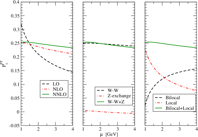
Figure 9: Evaluation of the charm quark contribution $P_{c}^{\mathrm{PT}}$ at the unphysical charm quark mass $m_{c}(\mbox{2 GeV})=863$ MeV following the procedure given in Ref. Buras et al. (2006). In the left-hand panel, we show the scale ($\mu$) dependence of total contribution $P_{c}^{\mathrm{PT}}(\mu)$ at the LO (black dashed curve), NLO (red dash-dotted curve) and NNLO (green solid curve). In the middle panel, we show the NNLO result for the $P_{c}^{\mathrm{PT}}(\mu)$ by splitting it into the $W$-$W$ ($P_{c}^{WW}$) and Z-exchange ($P_{c}^{Z}$) contributions. In the right-hand panel, we compare the bilocal and local contributions as a function of the scale $\mu$; both include the NNLO corrections.

In Fig. 9, the bilocal contribution is estimated using the perturbation theory by integrating out the charm quark field. We question whether perturbation theory works well at the scale of $\mu=O(m_{c})$. We therefore replace the $r_{AB}^{\overline{\mathrm{MS}}}$ term by the nonperturbative evaluation of the bilocal matrix element together with a perturbative matching from RI/SMOM scheme to $\overline{\mathrm{MS}}$ scheme. The results are presented in Sec. VI.

V.5 Determination of the $Y_{AB}(\mu,\mu_{0})$

The relation between the $\overline{\mathrm{MS}}$ and RI/SMOM bilocal operators takes the form given in Eq. (6) which we rewrite here for the reader’s convenience:

$$\{Q_{A}^{\overline{\mathrm{MS}}}Q_{B}^{\overline{\mathrm{MS}}}\}^{\overline{\mathrm{MS}}}_{\mu}=Z_{A}^{\mathrm{RI}\to\overline{\mathrm{MS}}}(\mu/\mu_{0})Z_{B}^{\mathrm{RI}\to\overline{\mathrm{MS}}}(\mu/\mu_{0})\{Q_{A}Q_{B}\}^{\mathrm{RI}}_{\mu_{0}}+Y_{AB}(\mu,\mu_{0})Q_{0}^{\mathrm{RI}}(\mu_{0}),$$ (85)

where $\mu$ and $\mu_{0}$ are the $\overline{\mathrm{MS}}$ and RI/SMOM renormalization scales respectively. For compactness of notation, we have written Eq. (85) as if there is no mixing of the operators $Q_{A}$ and $Q_{B}$ with other operators. When, as in the case of the $Z$-exchange diagrams, there is a mixing then the renormalization constants become matrices, e.g. $Z_{A}Q_{A}\to Z_{AC}Q_{C}$.

In order to determine $Y_{AB}(\mu,\mu_{0})$ we calculate the amputated Green’s functions for both sides of Eq. (85) at $p_{i}^{2}=\mu_{0}^{2}$ and impose the renormalization condition Eq. (66) so that:

$$\bigl{\langle}\{Q_{A}^{\overline{\mathrm{MS}}}Q_{B}^{\overline{\mathrm{MS}}}\}^{\overline{\mathrm{MS}}}_{\mu}\bigr{\rangle}_{p_{i}^{2}=\mu_{0}^{2}}=\frac{Z_{q}^{\mathrm{RI}}(\mu_{0})}{Z_{q}^{\overline{\mathrm{MS}}}(\mu)}\,Y_{AB}(\mu,\mu_{0})\,\bigl{\langle}Q_{0}^{\mathrm{RI}}\bigr{\rangle}_{p_{i}^{2}=\mu_{0}^{2}}.$$ (86)

Here $Z_{q}^{\mathrm{RI}}$ and $Z_{q}^{\overline{\mathrm{MS}}}$ are the quark’s wave function renormalization constant. In the Landau gauge and setting the renormalization scales of both $\overline{\mathrm{MS}}$ and RI/SMOM schemes to be equal $\mu=\mu_{0}$, we have $Z_{q}^{\mathrm{RI}}/Z_{q}^{\overline{\mathrm{MS}}}=1+O(\alpha_{s}^{2})$ Sturm et al. (2009). On the right-hand side of Eq. (86), the definition of the RI/SMOM renormalization scheme implies that $\bigl{\langle}Q_{0}^{\mathrm{RI}}\bigr{\rangle}_{p_{i}^{2}=\mu_{0}^{2}}=\bigl{\langle}Q_{0}\bigr{\rangle}_{p_{i}^{2}=\mu_{0}^{2}}^{(0)}$, where the superscript $(0)$ denotes the tree-level amputated Green’s function.

We write $Y_{A,B}(\mu,\mu_{0})\equiv Y_{A,B}(\mu,0)+\Delta Y_{AB}(\mu,\mu_{0})$, where $Y_{A,B}(\mu,0)$ is exactly given by the $r_{AB}^{\overline{\mathrm{MS}}}(\mu)$ discussed in Sec. V.4. We present the determination of the $\Delta Y_{AB}$ at $O(\alpha_{s}^{0})$ in Appendix B and the results are given in Eqs. (119), (126) and (130).

In our analysis, we take the expression for $r_{AB}^{\overline{\mathrm{MS}}}(\mu)$ from Ref. Buras et al. (2006), where it has been calculated at $O(\alpha_{s}^{1})$. We estimate $\Delta Y_{AB}(\mu,\mu_{0})$ at $O(\alpha_{s}^{0})$. As we will show later, $\Delta Y_{AB}(\mu,\mu_{0})$ is of comparable size to $r_{AB}^{\overline{\mathrm{MS}}}(\mu)$. Thus the inclusion of the scale dependence of the charm quark mass is important for the determination of both $\Delta Y_{AB}(\mu,\mu_{0})$ and $r_{AB}^{\overline{\mathrm{MS}}}(\mu)$. In $r_{AB}^{\overline{\mathrm{MS}}}(\mu)$, the running charm quark mass only depends on the $\overline{\mathrm{MS}}$ scale $\mu$, while in $\Delta Y_{AB}(\mu,\mu_{0})$, the charm quark mass also depends on the RI/SMOM scale $\mu_{0}$. For simplicity, we choose $\mu=\mu_{0}$. Note that the mass renormalization conversion factors from the RI/SMOM scheme to the $\overline{\mathrm{MS}}$ scheme have been calculated to two-loop order. At $\mu=\mu_{0}\geq\mbox{2 GeV}$ these conversion factors only deviate from 1 by a few percent Gorbahn and Jager (2010). We thus neglect the RI/SMOM scale dependence and simply use the $\overline{\mathrm{MS}}$ charm quark mass from Eq. (77) for $\Delta Y_{AB}(\mu,\mu)$.

In Fig. 10, we show the contributions to $C_{A}^{\overline{\mathrm{MS}}}C_{B}^{\overline{\mathrm{MS}}}\Delta Y_{AB}(\mu,\mu_{0})$, $C_{A}^{\overline{\mathrm{MS}}}C_{B}^{\overline{\mathrm{MS}}}r_{AB}^{\overline{\mathrm{MS}}}(\mu)$ and $C_{A}^{\overline{\mathrm{MS}}}C_{B}^{\overline{\mathrm{MS}}}Y_{AB}(\mu,\mu_{0})$ as a function of $\mu=\mu_{0}$ from the $W$-$W$ diagrams (left panel) and the $Z$-exchange diagrams (right panel). Since the magnitude of $\Delta Y_{AB}(\mu,\mu)$ is comparable to $r_{AB}^{\overline{\mathrm{MS}}}(\mu)$, it will be important in future calculations to include the $O(\alpha_{s})$ correction and the RI/SMOM scale dependence of the charm quark mass running in $\Delta Y_{AB}(\mu,\mu_{0})$. Another observation from Fig. 10 is that the $\ln\frac{\mu^{2}}{m_{c}^{2}}$ dependence, present in each of the terms $\Delta Y_{AB}(\mu,\mu)$ and $r_{AB}^{\overline{\mathrm{MS}}}(\mu)$, cancels at $O(\alpha_{s}^{0})$ in the combination $r_{AB}^{\overline{\mathrm{MS}}}(\mu)+\Delta Y_{AB}(\mu,\mu)$ (see also Eq. (B)) .

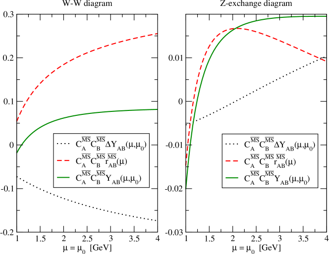
Figure 10: Contributions to $\Delta Y_{AB}(\mu,\mu_{0})$, $r_{AB}^{\overline{\mathrm{MS}}}(\mu)$ and $Y_{AB}(\mu,\mu_{0})$, multiplied by the corresponding Wilson Coefficients, from the $W$-$W$ diagrams (left panel) and $Z$-exchange diagrams (right panel). They are shown as a function of $\mu=\mu_{0}$.

VI Lattice results and a discussion of systematic uncertainties

In the previous sections we have discussed and computed all the ingredients necessary to determine the decay amplitude for the process $K^{+}\to\pi^{+}\nu\bar{\nu}$. Before presenting our final result for the amplitude, we briefly summarise how these ingredients are combined to obtain this result. We started in Sec. III with a calculation of the matrix elements of the local and bilocal lattice operators relevant for the rare kaon decays. These computations are naturally non-perturbative. In the determination of the matrix elements of bilocal operators new ultraviolet divergences appear when the two local operators $Q_{A}$ and $Q_{B}$ which comprise the bilocal operator approach each other. We discuss the subtraction of these additional divergences in Sec. IV, introducing and determining the subtraction constants $X_{AB}^{\mathrm{lat}}(\mu_{0},a)$ (see Eqs. (66) and (67)). By subtracting these divergences, we define and determine non-perturbatively the matrix element of the bilocal operators renormalised in the RI/SMOM scheme. Since Wilson Coefficients are generally calculated in the $\overline{\mathrm{MS}}$ scheme, we need to convert the RI/SMOM operators into those in the $\overline{\mathrm{MS}}$ scheme and this is necessarily a perturbative calculation, which we describe in Sec. V. The $\mathrm{RI}\to\overline{\mathrm{MS}}$ conversion of the bilocal operators is characterized by the constants $Y_{AB}(\mu,\mu_{0})$ (see Eq. (85)). In this way we obtain the matrix elements of the bilocal operators in the $\overline{\mathrm{MS}}$ scheme without “integrating out” the charm quark. This matrix elements can be written generically in terms of the individual ingredients as follows:

$${\mathcal{A}}_{\mathrm{Bilocal}}^{\overline{\mathrm{MS}}} \equiv \langle\pi^{+}\nu\bar{\nu}|\{C_{A}^{\overline{\mathrm{MS}}}Q_{A}^{\overline{\mathrm{MS}}}C_{B}^{\overline{\mathrm{MS}}}Q_{B}^{\overline{\mathrm{MS}}}\}^{\overline{\mathrm{MS}}}_{\mu}|K^{+}\rangle$$ (87)

$$= C_{A}^{\mathrm{lat}}C_{B}^{\mathrm{lat}}\langle\pi^{+}\nu\bar{\nu}|\{Q_{A}^{\mathrm{lat}}Q_{B}^{\mathrm{lat}}\}^{\mathrm{lat}}_{a}|K^{+}\rangle$$

$$\hskip 10.84006pt-C_{A}^{\mathrm{lat}}C_{B}^{\mathrm{lat}}X_{AB}^{\mathrm{lat}}(\mu_{0},a)\langle\pi^{+}\nu\bar{\nu}|Q_{0}^{\mathrm{lat}}|K^{+}\rangle+C_{A}^{\overline{\mathrm{MS}}}C_{B}^{\overline{\mathrm{MS}}}Y_{AB}(\mu,\mu_{0})\langle\pi^{+}\nu\bar{\nu}|Q_{0}^{\mathrm{RI}}|K^{+}\rangle$$

$$= i\,\left[F_{\mathrm{4pt}}(\Delta,s)-2Z_{V}^{-1}C_{A}^{\mathrm{lat}}C_{B}^{\mathrm{lat}}X_{AB}^{\mathrm{lat}}(\mu_{0},a)f_{+}(s)+2C_{A}^{\overline{\mathrm{MS}}}C_{B}^{\overline{\mathrm{MS}}}Y_{AB}(\mu,\mu_{0})f_{+}(s)\right]$$

$$\hskip 10.84006pt\times\left[\bar{u}(p_{\nu}){\not{p}}_{K}(1-\gamma_{5})]v(p_{\bar{\nu}})\right]\,.$$

Depending on the choice of the operators $Q_{\{A,B\}}$, Eq. (87) represents contributions to the $W$-$W$ or $Z$-exchange diagrams. The scalar amplitude $F_{\mathrm{4pt}}(\Delta,s)$ is given by $F_{WW}(\Delta,s)$ for $W$-$W$ diagram and $2F_{+}^{Z,i}(s)$ ($i=V,A$) for the $Z$-exchange diagram. The variables $\Delta$ and $s$ are defined in Eq. (8). The $K_{\ell 3}$ form factor $f_{+}(s)$ is defined in Eq. (23). The results for $f_{+}(s)$, $F_{WW}(\Delta,s)$ and $F_{+}^{Z,i}(s)$ have been given in Tables 2, 3 and 4 respectively. The results for $X_{AB}^{\mathrm{lat}}(\mu_{0},a)$ in the range $\mbox{1\, GeV}\leq\mu_{0}\leq{4}$ GeV are listed in Table 6 and $Z_{V}=Z_{A}=0.7163(14)$. For the $Z$-exchange diagrams in Table 6 we also give the results with the corresponding Wilson Coefficients (labelled $C_{1}^{\mathrm{lat}}Q_{1}+C_{2}^{\mathrm{lat}}Q_{2}$). The results for $Y_{AB}(\mu,\mu_{0})$ for $\mbox{1 GeV}\leq\mu=\mu_{0}\leq\mbox{4 GeV}$ are shown in Fig. 10.

It is convenient to define the ratio $R(\Delta,s)$:

$$R(\Delta,s)\equiv\frac{F_{\mathrm{4pt}}(\Delta,s)}{2f_{+}(s)}.$$ (88)

Since in this calculation we use use a single choice of momenta (see Eq. (13)), we are not able to determine the $\Delta$ and $s$ dependence of $R(\Delta,s)$. Here we simply neglect this momentum dependence.

The bilocal matrix element can be written as

$${\mathcal{A}}_{\mathrm{Bilocal}}^{\overline{\mathrm{MS}}} \simeq i\,\left[R(\Delta,s)-Z_{V}^{-1}C_{A}^{\mathrm{lat}}C_{B}^{\mathrm{lat}}X_{AB}^{\mathrm{lat}}(\mu_{0},a)+C_{A}^{\overline{\mathrm{MS}}}C_{B}^{\overline{\mathrm{MS}}}Y_{AB}\right]$$ (89)

$$\hskip 10.84006pt\times\left[2f_{+}(s)\bar{u}(p_{\nu}){\not{p}}_{K}(1-\gamma_{5})v(p_{\bar{\nu}})\right]\,,$$

where the $\simeq$ symbol on the first line reminds us that the momentum dependence of $R(\Delta,s)$ has been neglected. We denote the sum of the ${\mathcal{A}}_{\mathrm{Bilocal}}^{\overline{\mathrm{MS}}}$ from the $WW$ and $Z$-exchange diagrams by ${\mathcal{A}}_{\mathrm{Bilocal}}^{\overline{\mathrm{MS}},\textrm{TOT}}$ and combine it with the contribution from the matrix element of the local operator

$${\mathcal{A}}_{\mathrm{Local}}^{\overline{\mathrm{MS}}}=i\,\left[C_{0,Z}^{\overline{\mathrm{MS}}}(\mu)+\frac{1}{3}\sum_{\ell,\mu,\tau}C_{0,WW}^{\overline{\mathrm{MS}}}(\mu)\right]\,\left[2f_{+}(s)\bar{u}(p_{\nu}){\not{p}}_{K}(1-\gamma_{5})v(p_{\bar{\nu}})\right]$$ (90)

to obtain the total charm quark contributions to the decay amplitude. It is conventional to relate the ${\mathcal{A}}_{\mathrm{Bilocal}}^{\overline{\mathrm{MS}},\textrm{TOT}}$ and ${\mathcal{A}}_{\mathrm{Local}}^{\overline{\mathrm{MS}}}$ to $P_{c}$ through

$${\mathcal{A}}_{\mathrm{Bilocal}}^{\overline{\mathrm{MS}},\textrm{TOT}}+{\mathcal{A}}_{\mathrm{Local}}^{\overline{\mathrm{MS}}}=\frac{\lambda^{4}}{\pi^{2}}M_{W}^{2}P_{c}\left[2f_{+}(s)\bar{u}(p_{\nu}){\not{p}}_{K}(1-\gamma_{5})v(p_{\bar{\nu}})\right]\,.$$ (91)

We now separate $P_{c}$ into two parts: the standard charm-quark estimate $P_{c}^{\mathrm{PT}}$ calculated using perturbation theory (see Eq. (84)) and a difference between the full non-perturbative lattice result and the perturbative estimate, $P_{c}-P_{c}^{\mathrm{PT}}$

$$P_{c}-P_{c}^{\mathrm{PT}}=\frac{1}{\lambda^{4}}\frac{\pi^{2}}{M_{W}^{2}}\left[R(\Delta,s)-Z_{V}^{-1}C_{A}^{\mathrm{lat}}C_{B}^{\mathrm{lat}}X_{AB}^{\mathrm{lat}}(\mu_{0},a)+C_{A}^{\overline{\mathrm{MS}}}C_{B}^{\overline{\mathrm{MS}}}\Delta Y_{AB}(\mu,\mu_{0})\right].$$ (92)

In Fig. 11 we show the unrenormalized quantity $\frac{1}{\lambda^{4}}\frac{\pi^{2}}{M_{W}^{2}}R(\Delta,s)$ (gray band), the RI-renormalized quantity $\frac{1}{\lambda^{4}}\frac{\pi^{2}}{M_{W}^{2}}[R(\Delta,s)-Z_{V}^{-1}C_{A}^{\mathrm{lat}}C_{B}^{\mathrm{lat}}X_{AB}^{\mathrm{lat}}(\mu_{0},a)]$ (red circle), the total charm contribution $P_{c}$ (blue diamond) and the difference $P_{c}-P_{c}^{\mathrm{PT}}$ (green square) as a function of $\mu=\mu_{0}$. From the left to right, three panels show the results for the $W$-$W$ diagrams, the $Z$-exchange diagrams and their sum.

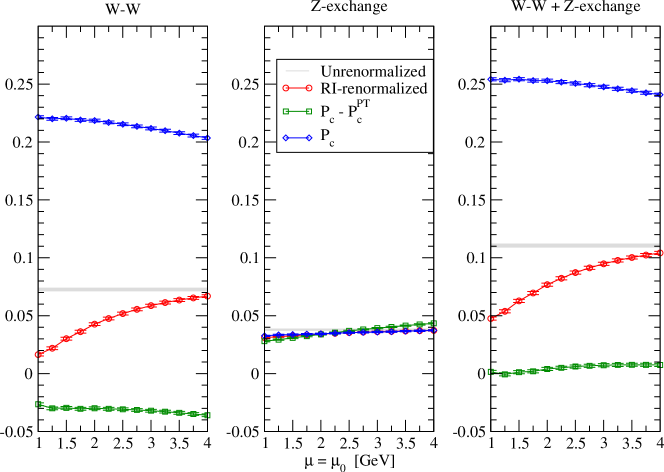
Figure 11: The unrenormalized lattice matrix elements $\frac{1}{\lambda^{4}}\frac{\pi^{2}}{M_{W}^{2}}R(\Delta,s)$ (indicated by the gray band), the RI-renormalized matrix elements $\frac{1}{\lambda^{4}}\frac{\pi^{2}}{M_{W}^{2}}[R(\Delta,s)-Z_{V}^{-1}C_{A}^{\mathrm{lat}}C_{B}^{\mathrm{lat}}X_{AB}^{\mathrm{lat}}(\mu_{0},a)]$ (red circles), the total charm-quark contribution $P_{c}$ (blue diamonds) and the difference $P_{c}-P_{c}^{\mathrm{PT}}$ (green squares) are shown as a function of $\mu=\mu_{0}$. From left to right, the three panels show the contribution of the $W$-$W$ diagrams, the $Z$-exchange diagram and the total, i.e. the sum of the two.

At scales $\mu=\mu_{0}=1,2,3,4$ GeV, we obtain respectively

$$P_{c} = 0.2541(13),0.2529(13),0.2476(13),0.2408(13)\,,$$

$$P_{c}-P_{c}^{\mathrm{PT}} = 0.0015(13),0.0040(13),0.0072(13),0.0074(13)\,.$$ (93)

As shown in Tables 3 and 4 the statistical errors in the unrenormalized bilocal matrix are about 1-2%. When these uncertainties propagate to $P_{c}$, they only appear as sub-percent effects, since in $P_{c}$ the largest contribution comes from the perturbation theory.

There is a curious cancellation evident in Fig. 11. The figure shows that the contributions from each of the $WW$ and $Z$-exchange diagrams to $P_{c}-P_{c}^{\textrm{PT}}$ clearly deviate from 0 due to non-perturbative effects. However, they have the opposite sign and as a result there is a significant cancellation. For illustration, at $\mu=\mu_{0}$=2 GeV, the contribution to $P_{c}-P_{c}^{\textrm{PT}}$ from the $WW$ diagram is $-2.99(12)\times 10^{-2}$ and from the $Z$-exchange diagram is $3.39(6)\times 10^{-2}$. The sum of the two contributions is about 10 times smaller than each contribution separately. It will be very interesting to check whether such a cancellation persists as the masses of the quarks are changed to their physical values.

VI.1 Systematic effects

Although the statistical errors are well under control, in order to obtain a precise calculation of the long-distance contribution to the $K^{+}\to\pi^{+}\nu\bar{\nu}$ decay amplitude, it is important also to have a good understanding of the systematic uncertainties. In this subsection we discuss some of the principle sources of these uncertainties.

VI.1.1 The RI/SMOM and $\overline{\mathrm{MS}}$ scale dependence

As can be seen from Eq. (VI), the systematic uncertainty arising from the scale dependence is much larger than the statistical error. There are two main sources of this scale dependence. At small scales $\mu=\mu_{0}\approx 1$ GeV, we expect that higher-order QCD corrections, which are not included in our calculation of $\Delta Y_{AB}$, will cause a sizeable effect. At larger scales, $\mu=\mu_{0}\approx 4$ GeV say, we expect that lattice artifacts might be significant. We quote the results for $P_{c}$ and $P_{c}^{\mathrm{PT}}$ as

$$P_{c}=0.2529(13)(32),\quad P_{c}-P_{c}^{\mathrm{PT}}=0.0040(13)(32)\,$$ (94)

where the central values correspond to the scale $\mu=\mu_{0}=2$ GeV. The first error is statistical and the second an estimate of the error implied by the residual scale dependence of $P_{c}$, in the range 1 GeV$<\mu=\mu_{0}<3$ GeV.

VI.1.2 Contributions from disconnected diagrams

The calculation of disconnected diagrams usually suffers from large noise. This is also the case for the calculation of the rare kaon decay form factors, where the uncertainty of the disconnected diagrams is about 10-30% while for the connected diagrams, the uncertainty is at the level of few percent. This can be seen from Table 4. Fortunately, the size of the form factor from the disconnected diagrams, $F_{0}^{Z,A,disc}(s_{\mathrm{max}})=6.0(1.2)\cdot 10^{-4}$, is only a few percent of that from the connected diagram. It only contributes to $P_{c}$ at the level of 0.4%. Here we should point out that since we do not use twisted boundary conditions for disconnected diagrams, we only calculate them with the mesons at rest, ${\bf p}_{K}={\bf p}_{\pi}={\bf 0}$. We thus determine $F_{0}^{Z,A,disc}(s_{\textrm{max}})$ instead of $F_{+}^{Z,A,disc}(s)$. If we assume that $F_{0}^{Z,A}(s_{\textrm{max}})$ is a good approximation to $F_{+}^{Z,A}(s)$, then the disconnected diagrams only contribute to $P_{c}$ at a negligible level. Recall that at $s=s_{\textrm{max}}$ the vector current does not contribute to the amplitude.

VI.1.3 Finite volume effects

As explained in Ref. Christ et al. (2016a), the main finite volume (FV) effects in the lattice calculation of the $K^{+}\to\pi^{+}\nu\bar{\nu}$ decay amplitude arise from the $K^{+}\to\pi^{+}\pi^{0}\to\pi^{+}\nu\bar{\nu}$ process for the $Z$-exchange diagrams and $K^{+}\to\pi^{0}\ell^{+}\nu\to\pi^{+}\nu\bar{\nu}$ for the $W$-$W$ diagrams. The transitions $K^{+}\to 3\pi\to\pi^{+}\nu\bar{\nu}$ and $K^{+}\to 2\pi\ell^{+}\nu\to\pi^{+}\nu\bar{\nu}$ can be neglected due to significant phase space suppression. We therefore exclude them from our discussion.

For the transition $K^{+}\to\pi^{+}\pi^{0}$, since the pion mass used in this calculation is $420$ MeV (so that $m_{K}<2m_{\pi}$), no significant finite-volume effects are expected. Nevertheless, we have calculated two-pion scattering energy in the isospin $I=2$ channel as well as the $K^{+}\to\pi^{+}\pi^{0}$ and $\pi^{+}\pi^{0}\to\pi^{+}$ transition amplitude. There are no expected difficulties to evaluating the potentially large finite-volume effects by using Lellouch-Lüscher formula when we repeat the calculation at physical quark masses (and therefore with $m_{K}>2m_{\pi}$) in the future.

Here we focus on the transition $K^{+}\to\pi^{0}\ell^{+}\nu\to\pi^{+}\nu\bar{\nu}$ and denote the potentially large, i.e. non-exponential, FV correction by $A_{\textrm{FV}}^{\pi^{0}\ell^{+}}=A_{WW}(L)-A_{WW}(\infty)$, where $A_{WW}(L)$ and $A_{WW}(\infty)$ are the contributions to the amplitude from the $WW$ diagrams in finite and infinite volumes respectively. The label $\pi^{0}\ell^{+}$ indicates that the correction comes from the $\pi^{0}\ell^{+}$ intermediate state; see Fig. 2. The neutrino plays no rôle here beyond determining the energy-momentum of the $\pi^{0}\ell^{+}$ pair. $A_{\textrm{FV}}^{\pi^{0}\ell^{+}}$ can be expressed as Christ et al. (2016a)

$$A_{\textrm{FV}}^{\pi^{0}\ell^{+}} = \left(\frac{1}{L^{3}}\sum_{\vec{k}}\int\frac{dk_{0}}{2\pi}-{\mathcal{P}}\int\frac{d^{4}k}{(2\pi)^{4}}\right)\left\{A_{\alpha}^{K^{+}\to\pi^{0}}(p_{K},k)\frac{1}{k^{2}+m_{\pi}^{2}}A_{\beta}^{\pi^{0}\to\pi^{+}}(k,p_{\pi})\right\}$$ (95)

$$\hskip 42.67912pt\times\left\{\bar{u}(p_{\nu})\gamma^{\alpha}(1-\gamma_{5})\frac{i({\not{P}}-{\not{k}})+m_{\bar{\ell}}}{(P-k)^{2}+m_{\bar{\ell}}^{2}}\gamma^{\beta}(1-\gamma_{5})v(p_{\bar{\nu}})\right\},$$

where $k$ is the momentum carried by the intermediate $\pi^{0}$ and $P=p_{K}-p_{\nu}$ is the total momentum flowing into the $\pi^{0}$-$\ell^{+}$ loop. $A_{\alpha}^{K^{+}\to\pi^{0}}$ and $A_{\beta}^{\pi^{0}\to\pi^{+}}$ represent the transition matrix elements indicated by the superscript and $\alpha,\,\beta$ are the Lorentz indices of the weak currents.

The detailed steps needed to evaluate $A_{\textrm{FV}}^{\pi^{0}\ell^{+}}$ are given in Appendix C. Here we only discuss the results. For our current ensemble, with $m_{\pi}=420$ MeV, only the $\ell^{+}=e^{+}$ state can satisfy the on-shell condition and thus suffers from the non-exponential FV corrections. Our estimate of the FV correction to the scalar amplitude for the electron mode is $F_{WW}^{e}(L)-F_{WW}^{e}(\infty)=1.528\cdot 10^{-2}$, which is about 14% of the $F_{WW}^{e}(L)$ as given in Table 3. When this FV correction propagates to $P_{c}$, it amounts approximately to approximately a 2% contribution. After including this FV correction, we write the results for $P_{c}$ and $P_{c}-P_{c}^{\mathrm{PT}}$ as

$$P_{c}=0.2529(\pm 13)(\pm 32)(-45),\quad P_{c}-P_{c}^{\mathrm{PT}}=0.0040(\pm 13)(\pm 32)(-45).$$ (96)

Since the calculations of the FV corrections require the determination of $A_{\alpha}^{K^{+}\to\pi^{0}}$ and $A_{\beta}^{\pi^{0}\to\pi^{+}}$, which we can only estimate at present, we choose not to decrease the central values in Eq. (96) but to include the estimate of the FV corrections in the uncertainty. In general, the FV corrections depend on the lattice size $L$ and how the momenta for the intermediate pion and lepton are assigned and one needs to examine them for each case. In the future, when simulations are performed with physical quark masses, it will be possible to use the calculated or measured values of the $K_{\ell 3}$ and pion form factors at the corresponding momenta to determine the FV corrections reliably.

VI.1.4 The momentum dependence

Using the effective Hamiltonian ${\mathcal{H}}_{\mathrm{eff},0}$ in Eq. (1) and the definition of $P_{c}$ in Eq. (91), one can write the $K^{+}\to\pi^{+}\nu\bar{\nu}$ decay amplitude as follows

$$\mathcal{A}(K^{+}\to\pi^{+}\nu\bar{\nu}) = \frac{G_{F}}{\sqrt{2}}\frac{\alpha\lambda^{5}}{2\pi\sin^{2}\theta_{W}}\sum_{\ell=e,\mu,\tau}\left(\frac{\lambda_{t}}{\lambda^{5}}X_{t}(x_{t})+\frac{\lambda_{c}}{\lambda}P_{c}\right)$$ (97)

$$\hskip 10.84006pt\times 2f_{+}(s)\bar{u}(p_{\nu}){\not{p}}_{K}(1-\gamma_{5})v(p_{\bar{\nu}}),$$

where $X_{t}(x_{t})$ and $P_{c}$ are the top and charm quark contributions, respectively and $f_{+}(s)$ is the $K_{\ell 3}$ form factor. Note that the charm quark contribution $P_{c}$ generically depends on two variables $\Delta$ and $s$. In Eq. (88) we have taken the ratio between the bilocal matrix element and local matrix element and assume this ratio does not have a significant $\Delta$ and $s$ dependence. As a consequence, $P_{c}$ in Eq. (97) is approximated by a constant. We now examine under what circumstance this is a good approximation.

With this aim in mind, we write out the explicit $\Delta$ and $s$ dependence for $\mathcal{A}(K^{+}\to\pi^{+}\nu\bar{\nu})$ and $P_{c}$. Using the phase space factor for three-body decays Patrignani et al. (2016), the decay width for $K^{+}\to\pi^{+}\nu\bar{\nu}$ can be written as

$$\Gamma[K^{+}\to\pi^{+}\nu\bar{\nu}]=\frac{1}{2^{10}\pi^{4}m_{K}^{3}}\int_{0}^{s_{\mathrm{max}}}ds\,\Delta_{\mathrm{max}}\int d\Omega\,|\mathcal{A}(\Delta,s)|^{2}$$ (98)

where $d\Omega=\sin\theta\,d\phi\,d\theta$ is the element of solid angle of the neutrino’s momentum in the center-of-mass frame of the $\nu\bar{\nu}$ pair and $\theta$ indicates the angle between the momenta of the pion and neutrino in the same frame. We then have

$$s_{\mathrm{max}}=(m_{K}-m_{\pi})^{2},\quad\Delta_{\mathrm{max}}=\sqrt{(m_{K}^{2}+m_{\pi}^{2}-s)^{2}-4m_{K}^{2}m_{\pi}^{2}},\quad\Delta=\Delta_{\mathrm{max}}\cos\theta.$$ (99)

The square of the amplitude $|\mathcal{A}(\Delta,s)|^{2}$ is given by

$$|\mathcal{A}(\Delta,s)|^{2} \propto \left[\left(\frac{\mathrm{Im}\,\lambda_{t}}{\lambda_{5}}X_{t}(x_{t})\right)^{2}+\left(\frac{\mathrm{Re}\,\lambda_{c}}{\lambda}P_{c}(\Delta,s)+\frac{\mathrm{Re}\,\lambda_{t}}{\lambda^{5}}X_{t}(x_{t})\right)^{2}\right]$$ (100)

$$\hskip 10.84006pt\times 4f_{+}(s)^{2}\left[\Delta_{\mathrm{max}}^{2}-\Delta^{2}\right]\,,$$

where the factor $\Delta_{\mathrm{max}}^{2}-\Delta^{2}$ arises from the relation $|\bar{u}(p_{\nu}){\not{p}}_{K}(1-\gamma_{5})v(p_{\bar{\nu}})|^{2}=\Delta_{\mathrm{max}}^{2}-\Delta^{2}$.

Assuming that the $\Delta$ and $s$ dependence in $P_{c}(\Delta,s)$ is mild we perform a Taylor expansion writing

$$P_{c}(\Delta,s)=P_{c}(0,0)+b_{\Delta}\frac{\Delta}{m_{K}^{2}}+b_{s}\frac{s}{m_{K}^{2}}+\cdots.$$ (101)

Using this simple expansion as an input, the branching ratio of $K^{+}\to\pi^{+}\nu\bar{\nu}$ is proportional to

$$\mathrm{Br}[K^{+}\to\pi^{+}\nu\bar{\nu}]\propto 1+0.071\,b_{\Delta}^{2}+0.202\,b_{s}\,.$$ (102)

Here, we have used $X_{t}(x_{t})=1.481$, $P_{c}(0,0)=0.404$, $\mathrm{Im}\,\lambda_{t}=1.51\times 10^{-4}$, $\mathrm{Re}\,\lambda_{t}=-3.20\times 10^{-4}$ Buras et al. (2015), $\lambda=0.22537$ and the PDG values for $m_{K}$ and $m_{\pi}$ Patrignani et al. (2016). We also make the approximation that $\mathrm{Re}\,\lambda_{c}\simeq-\lambda$ and $f_{+}(s)\simeq 1$. If $|b_{\Delta}|<0.37$ and $|b_{s}|<0.05$, then the momentum dependence only amounts for a sub-percent effect.

Of course, since the present simulation was performed at a single choice of $(s,\Delta)$ we are unable to estimate the size of the parameters $b_{s}$ and $b_{\Delta}$. Nevertheless, the above discussion will be useful in our future studies (see Sec. VII) in which we will determine these parameters and use them to inform our choice of kinematics for simulations at physical quark masses.

VII Conclusions and future prospects

In this paper we have presented an exploratory lattice QCD calculation of the long-distance contribution to the $K^{+}\to\pi^{+}\nu\bar{\nu}$ decay amplitude with a pion mass of $m_{\pi}=420$ MeV and with a charm quark of mass $m_{c}^{\overline{\mathrm{MS}}}(\mbox{2 GeV})=863$ MeV. The main results have previously been reported in Ref. Bai et al. (2017). In this longer version we give the details explaining how the bilocal hadronic matrix elements are evaluated and how the three main technical difficulties can be overcome. These are:

1. the treatment of the additional ultraviolet divergences which arise in second order perturbation theory when two local operators approach each other;

2. the subtraction of the unphysical terms which appear in Euclidean space and which grow exponentially with the temporal extent of the region of integration over the separation between the two local operators;

3. the correction for potentially large, i.e. non-exponential, finite-volume effects.

By using 800 gauge configurations, the statistical uncertainty of the lattice result for $P_{c}$ is reduced to sub-percent level. We also make an analysis of the systematic errors, which gives us some guidance on how to control these uncertainties in future calculations. A curious feature of our results is that there is a very significant cancellation between the contributions from the $WW$ and $Z$-exchange diagrams to $P_{c}-P_{c}^{\textrm{PT}}$, see Fig. 11 and the related discussion. It will be very important and interesting to see if such a cancellation persists as the masses of the quarks are changed towards their physical values in the future simulations discussed below.

Because of the unphysical quark masses used in this simulation, it is premature to compare our current lattice result with perturbative calculations Buras et al. (2015) and the estimate of LD effects from Ref. Isidori et al. (2005). The technique presented in this work can readily be generalized to a future realistic calculation. Such a simulation requires both a small lattice spacing to accommodate a physically heavy charm quark, and a large volume to accommodate physically light pions. We foresee that within four years adequate resources will become available to make such a calculation possible with controlled systematic errors.

We end the discussion with our more immediate plans. We are currently performing a calculation with a lighter pion mass, $m_{\pi}=170$ MeV, on a $32^{3}\times 64$ ensemble. This will help us to control the uncertainty from the unphysical pion mass of 420 MeV which we are currently using and provide information about the $(\Delta,s)$ momentum dependence since the allowed momentum region will be larger.

To include the physical charm quark mass, a fine lattice spacing is required. We are planning to use a $64^{3}\times 128$ ensemble with an inverse lattice spacing of $1/a=2.38$ GeV and with physical values for the light, strange and charm quark masses. As mentioned above, accurate results with a complete systematic error budget should be available within three to four years, which matches well with the experimental schedule to measure precisely the $K^{+}\to\pi^{+}\nu\bar{\nu}$ branching ratio.

Appendix A Free lepton propagator using the overlap formalism

The internal lepton is treated as an overlap fermion in this calculation. We employ the overlap quark action from Refs. Capitani (2003); Aoki et al. (2008b), with the Dirac operator defined as

$$D(0) = \rho\,(1+\gamma_{5}\,\textmd{sgn}\,[H_{W}(-\rho)]),\quad H_{W}=\gamma_{5}D_{W}$$

$$D(m) = \left(1-\frac{m}{2\rho}\right)D(0)+m\,,$$ (103)

where $D_{W}$ is the Wilson Dirac operator. Here we set the Wilson parameter $r=1$. The parameter $\rho$ introduced into the overlap fermion action is equivalent to the five-dimensional domain wall height $M_{5}$ in the domain wall fermion action. $m$ is the lepton mass.

It is useful to write the propagator of the free overlap fermion in momentum space

$$S(p)=\frac{1}{2}\frac{(\rho-\frac{m}{2})X^{\dagger}(p)+(\rho+\frac{m}{2})\omega(p)}{\left(\rho^{2}+\frac{m^{2}}{4}\right)\omega(p)+\left(\rho^{2}-\frac{m^{2}}{4}\right)b(p)}\,,$$ (104)

where

$$X(p) = i\sum_{\mu}\gamma_{\mu}\sin p_{\mu}+r\sum_{\mu}(1-\cos p_{\mu})-\rho$$

$$b(p) = r\sum_{\mu}(1-\cos p_{\mu})-\rho$$

$$\omega(p) = \sqrt{\sum_{\mu}\sin^{2}p_{\mu}+\left(r\sum_{\mu}(1-\cos p_{\mu})-\rho\right)^{\!\!2}}\,.$$ (105)

When $0<\rho<2r$ there is no pole at $p_{4}=\pi+iE$, since

$$b(p)=\left(r(1+\cosh E)+r\sum_{i}(1-\cos p_{i})-\rho\right)>0$$ (106)

and the constraint $\omega(p)+b(p)=0$ (corresponding to the massless case) cannot be satisfied. Thus the fermion doubling problem is solved and the correct spectrum of massless fermions is obtained in the range $0<\rho<2r$. We therefore only need to consider the pole at $p=({\bf p},iE_{a})$, which satisfies the relation

$$\sum_{\mu}\sin^{2}p_{\mu}=-\frac{\rho^{2}m^{2}}{(\rho^{2}+m^{2}/4)^{2}}b^{2}(p)\equiv-\bar{m}^{2}b^{2}(p)\,.$$ (107)

We next perform the Fourier transform in the time direction and convert the propagator to the momentum-time representation

$$S({\bf p},t)=\int_{-\pi}^{\pi}\frac{dp_{4}}{2\pi}\,S({\bf p},p_{4})e^{ip_{4}t}.$$ (108)

Here the integral $\int_{-\pi}^{\pi}\frac{dp_{4}}{2\pi}$ is used to obtain the propagator with infinite time extension. $S({\bf p},t)$ can be determined using Cauchy integration. Note that the square root in $\omega(p)$ brings in two branch cuts, one from a starting point $+iE_{b}$ to $+i\infty$ and the other from $-iE_{b}$ to $-i\infty$, where $p=({\bf p},iE_{b})$ is the zero of $\omega(p)$. So the contour of the Cauchy integral should exclude these branch cuts as shown in Fig. 12. For $t>0$ we have

$$\int_{-\pi}^{\pi}\frac{dp_{4}}{2\pi}\,f(p_{4})=i\,\mathrm{res}\{f\}_{p_{4}=iE_{a}}+\int_{+iE_{b}+\epsilon}^{+i\infty+\epsilon}\frac{dp_{4}}{2\pi}\,f(p_{4})-\int_{+iE_{b}-\epsilon}^{+i\infty-\epsilon}\frac{dp_{4}}{2\pi}\,f(p_{4}),\quad$$ (109)

with $f(p_{4})=S({\bf p},p_{4})e^{ip_{4}t}$. In the first term on the right-hand side $\mathrm{res}\{f\}_{p_{4}=iE_{a}}$ is the residue of $f(p_{4})$ at the pole $p_{4}=iE_{a}$. For $t<0$, we can choose the contour along the branch cut $-iE_{b}$ to $-i\infty$ to determine $S({\bf p},t)$.

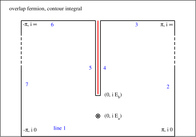
Figure 12: Line 1 is the contour of the integral on the left-hand side of Eq. (109) for $\mathbf{p}=\mathbf{0}$. For $t>0$, we close the contour in the upper-half plane picking up the residue of the pole at $p_{4}=iE_{a}$ and the contributions from the cut starting at $(0,iE_{B})$ leading to the three contributions on the right-hand side of Eq. (109).

The propagator $S({\bf p},t)$ can be written in two parts: the residue of the pole at $p_{4}=\pm iE_{a}$, $S_{a}({\bf p},t)$, and the contribution from the branch cuts, $S_{b}({\bf p},t)$. We first focus on the contribution from the pole and find

$$S_{a}({\bf p},t)=\frac{{\mathcal{C}}\left(\mathrm{sgn}(t)\sinh E_{a}\gamma_{t}-i\sum_{i}\sin p_{i}\gamma_{i}\right)+{\mathcal{M}}}{2{\mathcal{E}}}e^{-E_{a}|t|}\,,$$ (110)

with

$$\cosh E_{a} = \frac{\bar{m}^{2}r\left(\rho-r-r\sum_{i}(1-\cos p_{i})\right)+{\mathcal{U}}}{1-\bar{m}^{2}r^{2}}$$

$${\mathcal{E}} = \frac{\sinh E_{a}}{\rho}\left(\rho^{2}+\frac{m^{2}}{4}\right)\frac{{\mathcal{U}}}{\omega({\bf p},iE_{a})}$$

$${\mathcal{U}}^{2} = \bar{m}^{2}\left(\rho-r-r\sum_{i}(1-\cos p_{i})\right)^{\!\!2}+(1-\bar{m}^{2}r^{2})\left(1+\sum_{i}\sin^{2}p_{i}\right)$$

$${\mathcal{C}} = 1-\frac{m}{2\rho}$$

$${\mathcal{M}} = \frac{m}{\rho+m/2}\omega({\bf p},iE_{a}).$$ (111)

In order to achieve $O(a)$ improvement the propagator is modified as follows:

$$\hat{S}({\bf p},t)=\left(1-\frac{D(0)}{2\rho}\right)S({\bf p},t)=\frac{1}{{\mathcal{C}}}S({\bf p},t)-\frac{1}{2\rho-m}\,.$$ (112)

This modification cancels the coefficient ${\mathcal{C}}$ in $S({\bf p},t)$. The mass term ${\cal M}$ and $1/(2\rho-m)$ do not contribute to this calculation because of the $V-A$ structure of the two weak operators. We therefore write the modified propagator $\hat{S}_{a}({\bf p},t)$ as

$$\hat{S}_{a}({\bf p},t) \sim \frac{\mathrm{sgn}(t)\sinh E_{a}\gamma_{t}-i\sum_{i}\sin p_{i}\gamma_{i}}{2{\mathcal{E}}}e^{-E_{a}|t|}$$ (113)

$$= \frac{\sinh E_{a}}{{\mathcal{E}}}\frac{\mathrm{sgn}(t)\sinh E_{a}\gamma_{t}-i\sum_{i}\sin p_{i}\gamma_{i}}{2\sinh E_{a}}e^{-E_{a}|t|}\,.$$

We define the wave function normalization factor by $Z_{\ell}=\frac{\sinh E_{a}}{\mathcal{E}}\bigl{|}_{\bf p=0}$. As the lepton mass approaches $0$, $Z_{\ell}\to 1$. For large lepton masses, e.g. when $\ell=\tau$, we multiply $\hat{S}_{a}({\bf p},t)$ by $Z_{\ell}^{-1}$ in order to make the propagator have a closer form to the continuum one. Another subtelty is that at ${\bf p}=0$, the energy $E_{a}$ deviates from the input mass parameter $m$. For $\rho=r=1$, we have

$$m=2\operatorname{tanh}\frac{E_{a}}{2}\bigg{|}_{\bf p=0}.$$ (114)

We tune the parameter $m$ for each lepton, $e$, $\mu$ and $\tau$, to ensure that the pole mass $E_{a}$ at ${\bf p=0}$ takes the physical value of the mass of the lepton.

The branch-cut contribution is suppressed at large $t$. Its integral representation is

$$S_{b}({\bf p},t)=\int_{E_{b}}^{\infty}\frac{dE}{2\pi}\frac{(\rho-m/2)(\rho^{2}+m^{2}/4)\omega\sinh E}{(\rho^{2}+m^{2}/4)^{2}\omega^{2}+(\rho^{2}-m^{2}/4)^{2}b^{2}}\,e^{-E|t|}\,.$$ (115)

Appendix B Evaluation of $\textbf{RI}\boldsymbol{\to}\overline{\textbf{MS}}$ conversion for the bilocal operator: $Y_{AB}(\mu,\mu_{0})$

In this appendix we evaluate the amputated Green’s function in Eq. (63) using naive dimensional regularization (NDR) with a fully anticommuting $\gamma^{5}$. The external momentum $p_{i}$ are given by Eq. (62). Since the external legs are amputated, at $O(\alpha_{s}^{0})$ only the momentum $p=p_{\mathrm{loop}}$ enters as a parameter in the 4-momentum integral.

For the $W$-$W$ diagram, we have

$$\Gamma^{WW}(p) = \Gamma_{u}^{WW}(p)-\Gamma_{c}^{WW}(p)\quad\textrm{where}$$ (116)

$$\Gamma^{WW}_{q}(p) \equiv \mu^{\varepsilon}\int\frac{d^{D}k}{(2\pi)^{D}}\gamma_{\mu}^{L}S_{q}(-k)\gamma_{\nu}^{L}\otimes\gamma_{\mu}^{L}S_{\ell}(k+p)\gamma_{\nu}^{L},$$ (117)

$D$ is the number of space-time dimensions, $\varepsilon=4-D$ and the factor $\mu^{\varepsilon}$ ensures that $\Gamma_{q}^{WW}$ has the correct dimensions. In the integrand on the right-hand side of Eq. (117) $S_{q}(k)=\frac{1}{i{\not{k}}+m_{q}}$ is the quark propagator with $q=u,c$ and $S_{\ell}(k)=\frac{1}{i{\not{k}}+m_{\ell}}$ is the lepton propagator. The gamma matrix $\gamma_{\mu}^{L}$ ($\gamma_{\mu}^{R}$) is defined as $\gamma_{\mu}^{L}\equiv\gamma_{\mu}(1-\gamma_{5})$ ($\gamma_{\mu}^{R}\equiv\gamma_{\mu}(1+\gamma_{5})$).

As a result of the GIM cancellation in Eq. (116), $\Gamma^{WW}(p)$ is logarithmically divergent ($\Gamma^{WW}_{u}$ and $\Gamma^{WW}_{c}$ are separately quadratically divergent). The standard way to evaluate $\Gamma^{WW}_{q}$ requires the use of the $\gamma$ matrix algebra in the $D$ dimension. However, if we perform the subtraction $\Delta\Gamma^{WW}\equiv\Gamma^{WW}(p)-\Gamma^{WW}(0)$ then $\Delta\Gamma^{WW}$ is a finite quantity. We can then let $D\to 4$ and calculate $\Delta\Gamma^{WW}$ directly using the 4-dimensional $\gamma$-matrix algebra.

The conversion term $Y_{AB}^{WW}(\mu,\mu_{0})$ is given by

$$Y_{AB}^{WW}(\mu,\mu_{0})=\mu^{\varepsilon}\,\int\frac{d^{D}k}{(2\pi)^{D}}\frac{\mathrm{Tr}[\gamma_{\mu}^{L}S_{u}(-k)\gamma_{\nu}^{L}\gamma_{\rho}^{R}]\mathrm{Tr}[\gamma_{\mu}^{L}S_{\ell}(k+p)\gamma_{\nu}^{L}\gamma_{\rho}^{R}]}{\mathrm{Tr}[\gamma_{\mu}^{L}\gamma_{\rho}^{R}]\mathrm{Tr}[\gamma_{\mu}^{L}\gamma_{\rho}^{R}]}-\{u\to c\}\,,$$ (118)

where $\mu_{0}^{2}=p_{i}^{2}$. Here we retain our general notation with the operators denoted by $A$ and $B$ on the left hand side, but with the specific operators for the $W$-$W$ diagrams included on the right-hand side (see Eq. (18)).

At zero external momentum $Y_{AB}^{WW}(\mu,0)=r_{AB}^{WW}(\mu)$, where $r_{AB}^{WW}(\mu)$ is given by Eq. (83). The difference between $Y_{AB}^{WW}(\mu,\mu_{0})$ and $Y_{AB}^{WW}(\mu,0)$ is finite and we evaluate it at order $O(\alpha_{s}^{0})$:

$$\Delta Y_{AB}^{WW}(\mu,\mu_{0}) \equiv Y_{AB}^{WW}(\mu,\mu_{0})-Y_{AB}^{WW}(\mu,0)$$ (119)

$$= 16\left[\left(I_{1}(0,m_{\ell},p)-I_{1}(m_{c},m_{\ell},p)\right)-\left(I_{1}(0,m_{\ell},0)-I_{1}(m_{c},m_{\ell},0)\right)\right],$$

where $p^{2}=\mu_{0}^{2}$ and

$$I_{1}(m_{1},m_{2},p)\equiv\frac{1}{16\pi^{2}}\int_{0}^{1}dx\,(\Delta-A)\ln\frac{\Delta}{\mu^{2}}\,,$$ (120)

$x$ is a Feynman parameter, $\Delta=x(1-x)p^{2}+xm_{1}^{2}+(1-x)m_{2}^{2}$ and $A=2x(x-1)p^{2}-xm_{1}^{2}-(1-x)m_{2}^{2}$.

For the $Z$-exchange diagram with the insertion of the axial vector current, we evaluate the amputated Green’s function writing

$$\Gamma^{Z,A} = \Gamma^{Z,A}_{u}-\Gamma^{Z,A}_{c}$$

$$\Gamma_{q}^{Z,A} = \left\{\begin{array}[]{ll}q_{A}\,\mu^{\varepsilon}\int\frac{d^{D}k}{(2\pi)^{D}}\,\gamma_{\mu}^{L}S_{q}(k+p)\gamma_{\nu}\gamma_{5}S_{q}(k)\gamma_{\mu}^{L}\otimes\gamma_{\nu}^{L},&\leavevmode\nobreak\ \mbox{for the $Q_{2}$ operator}\\ -q_{A}\,\mu^{\varepsilon}\int\frac{d^{D}k}{(2\pi)^{D}}\,\mathrm{Tr}[\gamma_{\mu}^{L}S_{q}(k+p)\gamma_{\nu}\gamma_{5}S_{q}(k)]\gamma_{\mu}^{L}\otimes\gamma_{\nu}^{L},&\leavevmode\nobreak\ \mbox{for the $Q_{1}$ operator}\end{array}\right.$$ (123)

where $q_{A}=-T_{3}^{u}=-\frac{1}{2}$ and $T_{3}^{u}$ is the weak isospin for the up-type quarks.

Performing the projection and evaluating $\Delta Y_{AB}^{Z,A}\equiv Y_{AB}^{Z,A}(\mu,\mu_{0})-Y_{AB}^{Z,A}(\mu,0)$, we find

$$\Delta Y_{AB}^{Z,A}=\left\{\begin{array}[]{ll}2q_{A}\left[\left(I_{2}(0,p)-I_{2}(m_{c},p)\right)+I_{2}(m_{c},0)\right],&\leavevmode\nobreak\ \mbox{for the $Q_{2}$ operator}\\ 2q_{A}N_{c}\left[\left(I_{2}(0,p)-I_{2}(m_{c},p)\right)+I_{2}(m_{c},0)\right],&\leavevmode\nobreak\ \mbox{for the $Q_{1}$ operator}\end{array}\right.$$ (126)

where

$$I_{2}(m,p)=\frac{1}{16\pi^{2}}\int_{0}^{1}dx\,\left[3x(1-x)p^{2}+4m^{2}\right]\ln\frac{x(1-x)p^{2}+m^{2}}{\mu^{2}}.$$ (127)

For the insertion of the vector current, we can simply replace $\gamma_{\nu}\gamma_{5}\to\gamma_{\nu}$ and $q_{A}\to q_{V}=T_{3}^{u}-2Q_{\mathrm{em},u}\sin^{2}\theta_{W}$ in Eq. (B), where $Q_{\mathrm{em},u}$ is the electric charge for up-type quarks and $\theta_{W}$ is the Weinberg angle. We have

$$\Delta Y_{AB}^{Z,V}(\mu,\mu_{0})=\left\{\begin{array}[]{ll}-2q_{V}\left[\left(I_{3}(0,p)-I_{3}(m_{c},p)\right)+I_{3}(m_{c},0)\right],&\leavevmode\nobreak\ \mbox{for the $Q_{2}$ operator}\\ -2q_{V}N_{c}\left[\left(I_{3}(0,p)-I_{3}(m_{c},p)\right)+I_{3}(m_{c},0)\right],&\leavevmode\nobreak\ \mbox{for the $Q_{1}$ operator}\end{array}\right.$$ (130)

where

$$I_{3}(m,p)=\frac{1}{16\pi^{2}}\int_{0}^{1}dx\,3x(1-x)p^{2}\ln\frac{x(1-x)p^{2}+m^{2}}{\mu^{2}}.$$ (131)

Note that the contributions to $\Delta Y_{AB}$ are finite and $\log\mu^{2}$ cancels in each of the expressions in Eqs. (119), (126) and (130) at lowest order.

At large RI/SMOM scales, we have

$$\Delta Y_{AB}^{WW}(\mu,\mu_{0}) \xrightarrow[]{\mu_{0}^{2}\gg m_{c}^{2}} \frac{m_{c}^{2}}{\pi^{2}}\left(-\frac{x_{\ell}\ln x_{\ell}}{1-x_{\ell}}-\ln\frac{\mu_{0}^{2}}{m_{c}^{2}}\right)$$

$$\Delta Y_{AB}^{Z,A}(\mu,\mu_{0}) \xrightarrow[]{\mu_{0}^{2}\gg m_{c}^{2}} \frac{m_{c}^{2}}{4\pi^{2}}\left(-\frac{5}{4}+\ln\frac{\mu_{0}^{2}}{m_{c}^{2}}\right),\quad\mbox{for the $Q_{2}$ operator}$$

$$\Delta Y_{AB}^{Z,V}(\mu,\mu_{0}) \xrightarrow[]{\mu_{0}^{2}\gg m_{c}^{2}} q_{V}\frac{3}{8}\frac{m_{c}^{2}}{\pi^{2}},\quad\mbox{for the $Q_{2}$ operator}.$$ (132)

For the $Z$-exchange diagram, the results for the $Q_{1}$ operator are obtained by simply multiplying those for the $Q_{2}$ operator in Eq. (132) by a factor of $N_{c}$.

Combining $\Delta Y_{AB}(\mu,\mu_{0})$ with $r_{AB}^{\overline{\mathrm{MS}}}(\mu)$ and taking $\mu_{0}=\mu$ we have

$$Y_{AB}^{WW}(\mu,\mu_{0})\bigl{|}_{\mu=\mu_{0}} \xrightarrow[]{\mu_{0}^{2}\gg m_{c}^{2}} \frac{5}{4}\frac{m_{c}^{2}}{\pi^{2}}$$

$$Y_{AB}^{Z,A}(\mu,\mu_{0})\bigl{|}_{\mu=\mu_{0}} \xrightarrow[]{\mu_{0}^{2}\gg m_{c}^{2}} -\frac{1}{16}\frac{m_{c}^{2}}{\pi^{2}},\leavevmode\nobreak\ \mbox{for the $Q_{2}$ operator}$$

$$Y_{AB}^{Z,V}(\mu,\mu_{0})\bigl{|}_{\mu=\mu_{0}} \xrightarrow[]{\mu_{0}^{2}\gg m_{c}^{2}} q_{V}\frac{3}{8}\frac{m_{c}^{2}}{\pi^{2}},\leavevmode\nobreak\ \mbox{for the $Q_{2}$ operator}.$$ (133)

Appendix C Finite volume effects in the $W$-$W$ diagrams

We rewrite the expression in Eq. (95) in a more general form:

$$I_{FV}=I(L)-I(\infty)=\left(\frac{1}{L^{3}}\sum_{\vec{k}}\int\frac{dk_{4}}{2\pi}-{\mathcal{P}}\int\frac{d^{4}k}{(2\pi)^{4}}\right)\frac{f(k_{0},{\bf k})}{(k^{2}+m_{1}^{2})((P-k)^{2}+m_{2}^{2})},$$ (134)

where $P=p_{K}-p_{\nu}$, $m_{1}=m_{\pi}$ and $m_{2}=m_{\bar{\ell}}$ in our calculation. For the moving frame (${\bf P}\neq{\bf 0}$) and non-identical particles ($m_{1}\neq m_{2}$), the finite volume correction can be written as

$$I_{FV}=\frac{1}{2E^{*}}\sum_{lm}f_{lm}^{*}(p^{*})c_{lm}^{P}(p^{*})$$ (135)

where the superscript $*$ indicates the center-of-mass frame. The energy $E^{*}$ is the total energy in the center-of-mass frame, satisfying $E^{*2}=P_{0}^{2}-{\bf P}^{2}$, where the Minkowski and Euclidean energies, $P_{0}$ and $P_{4}$ respectively, are related by $P_{0}=-iP_{4}$. The momentum $p^{*}$ satisfies the on-shell condition $E^{*}=\sqrt{m_{1}^{2}+p^{*2}}+\sqrt{m_{2}^{2}+p^{*2}}$. The Lorentz boost factor $\gamma$ is given by $\gamma\equiv P_{0}/E^{*}$. Under the Lorentz transformation from the moving frame to the center-of-mass frame, the function $f({\bf k})$ changes as $f({\bf k})\to f^{*}({\bf k^{*}})$. The potentially large finite volume effects appear when the two particles in the intermediate state are both on-shell. In this case, the function $f({\bf k})$ corresponds to the on-shell physical transition and thus is Lorentz invariant: $f({\bf k})=f^{*}({\bf k^{*}})$. In Eq. (135) $f^{*}_{lm}(k^{*})$ is coefficient in the partial wave expansion of the function $f^{*}({\bf k^{*}})$:

$$f^{*}({\bf k}^{*})=\sum_{lm}f^{*}_{lm}(k^{*})k^{*l}Y_{lm}(\Omega_{\bf k^{*}}),\quad k^{*}\equiv|{\bf k^{*}}|=p^{*}.$$ (136)

The function $c_{lm}^{P}(p^{*})$ is given by Kim et al. (2005); Briceno and Davoudi (2013)

$$c_{lm}^{P}(p^{*})=\frac{1}{\gamma}\left(\frac{1}{L^{3}}\sum_{\bf k\in\frac{2\pi}{L}{\bf n}}-{\mathcal{P}}\int\frac{d^{3}{\bf k}}{(2\pi)^{3}}\right)\frac{|\hat{\bf k}|^{l}Y_{lm}(\Omega_{\hat{\bf k}})}{|\hat{\bf k}|^{2}-p^{*2}}\,,$$ (137)

where the momentum $\hat{\bf k}$ is defined as

$$\hat{\bf k}=\gamma^{-1}\left[{\bf k}_{\parallel}-\frac{\bf P}{2}\left(1+\frac{m_{1}^{2}-m_{2}^{2}}{E^{*2}}\right)\right]+{\bf k}_{\perp},\quad{\bf k}_{\parallel}=\frac{{\bf k}\cdot{\bf P}}{|{\bf P}|^{2}}{\bf P},\quad{\bf k}_{\perp}={\bf k}-{\bf k}_{\parallel}.$$ (138)

The subscripts $\parallel$ and $\perp$ refer to parallel to and perpendicular to $\mathbf{P}$ respectively. Each of the two terms in Eq. (137) is separately ultraviolet divergent but the difference is convergent. The divergence can be regulated by introducing an exponential factor $e^{\alpha(p^{*2}-|\hat{\bf k}|^{2})}$ with $\alpha>0$ to the summand/integrand in Eq. (137). By using the heat kernel method proposed by Lüscher Luscher (1991), one can evaluate $c_{lm}^{P}(p^{*})$ in the limit of $\alpha\to 0^{+}$.

Once $c_{lm}^{P}(p^{*})$ is determined, the remaining task is to evaluate $f_{lm}^{*}(k^{*})$. The scalar amplitude $f(\mathbf{k})$ is defined from the transition amplitude

$${\mathcal{A}}^{K^{+}\to\pi^{0}\ell^{+}\nu} = i\,A_{\alpha}^{K^{+}\to\pi^{0}}(p_{K},k)A_{\beta}^{\pi^{0}\to\pi^{+}}(k,p_{\pi})\bar{u}(p_{\nu})\gamma^{\alpha}(1-\gamma_{5})({\not{P}}-{\not{k}})\gamma^{\beta}(1-\gamma_{5})v(p_{\bar{\nu}})$$ (139)

$$= i\,f({\bf k})\,\bar{u}(p_{\nu}){\not{p}}_{K}(1-\gamma_{5})v(p_{\bar{\nu}})\,.$$

The scalar amplitude $f({\bf k})$ is then obtained from ${\mathcal{A}}_{K^{+}\to\pi^{0}\ell^{+}\nu}$ through the projection

$$f({\bf k})=\frac{\mathrm{Tr}[{\not{A}}^{K^{+}\to\pi^{0}}(1-\gamma_{5})({\not{P}}-{\not{k}}){\not{A}}^{\pi^{0}\to\pi^{+}}(1-\gamma_{5}){\not{p}}_{\bar{\nu}}{\not{p}}_{K}(1-\gamma_{5}){\not{p}}_{\nu}]}{\mathrm{Tr}[{\not{p}}_{K}(1-\gamma_{5}){\not{p}}_{\bar{\nu}}{\not{p}}_{K}(1-\gamma_{5}){\not{p}}_{\nu}]}.$$ (140)

We now make the following approximations: $A_{\alpha}^{K^{+}\to\pi^{0}}(p_{K},k)\simeq i(p_{K}+k)_{\alpha}$ and $A_{\beta}^{\pi^{0}\to\pi^{+}}(k,p_{\pi})\simeq i(p_{\pi}+k)_{\beta}$, which correspond to setting the $K_{\ell 3}$ and pion form-factors to 1. (In future simulations with physical quark masses these approximations can be relaxed by using the measured or computed form factors at the corresponding momentum transfers.) After performing the Lorentz boost, we have

$$f^{*}({\bf k}^{*})=\frac{-2\mathrm{Tr}\left[({\not{p}}_{K}^{*}+{\not{k}}^{*})({\not{P}}^{*}-{\not{k}}^{*})({\not{p}}_{\pi}^{*}+{\not{k}}^{*})(1-\gamma_{5}){\not{p}}_{\bar{\nu}}^{*}{\not{p}}_{K}^{*}(1-\gamma_{5}){\not{p}}_{\nu}^{*}\right]}{\mathrm{Tr}[{\not{p}}_{K}^{*}(1-\gamma_{5}){\not{p}}_{\bar{\nu}}^{*}{\not{p}}_{K}^{*}(1-\gamma_{5}){\not{p}}_{\nu}^{*}]}.$$ (141)

Finally, after performing the partial wave expansion for $f^{*}({\bf k}^{*})$, the finite volume corrections are given by Eq. (135).

References

- Bai et al. (2017) Z. Bai, N. H. Christ, X. Feng, A. Lawson, A. Portelli, and C. T. Sachrajda, Phys. Rev. Lett. 118, 252001 (2017), arXiv:1701.02858 [hep-lat] .
- Isidori et al. (2005) G. Isidori, F. Mescia, and C. Smith, Nucl.Phys. B718, 319 (2005), arXiv:hep-ph/0503107 [hep-ph] .
- Christ et al. (2016a) N. H. Christ, X. Feng, A. Portelli, and C. T. Sachrajda (RBC, UKQCD), Phys. Rev. D93, 114517 (2016a), arXiv:1605.04442 [hep-lat] .
- Buchalla and Buras (1994) G. Buchalla and A. J. Buras, Nucl. Phys. B412, 106 (1994), arXiv:hep-ph/9308272 [hep-ph] .
- Buchalla and Buras (1999) G. Buchalla and A. J. Buras, Nucl.Phys. B548, 309 (1999), arXiv:hep-ph/9901288 [hep-ph] .
- Inami and Lim (1981) T. Inami and C. Lim, Prog.Theor.Phys. 65, 297 (1981).
- Misiak and Urban (1999) M. Misiak and J. Urban, Phys.Lett. B451, 161 (1999), arXiv:hep-ph/9901278 [hep-ph] .
- Brod et al. (2011) J. Brod, M. Gorbahn, and E. Stamou, Phys.Rev. D83, 034030 (2011), arXiv:1009.0947 [hep-ph] .
- Buras et al. (2015) A. J. Buras, D. Buttazzo, J. Girrbach-Noe, and R. Knegjens, (2015), arXiv:1503.02693 [hep-ph] .
- Buras et al. (2005) A. Buras, M. Gorbahn, U. Haisch, and U. Nierste, Phys.Rev.Lett. 95, 261805 (2005), arXiv:hep-ph/0508165 [hep-ph] .
- Buras et al. (2006) A. J. Buras, M. Gorbahn, U. Haisch, and U. Nierste, JHEP 0611, 002 (2006), arXiv:hep-ph/0603079 [hep-ph] .
- Brod and Gorbahn (2008) J. Brod and M. Gorbahn, Phys.Rev. D78, 034006 (2008), arXiv:0805.4119 [hep-ph] .
- Mescia and Smith (2007) F. Mescia and C. Smith, Phys. Rev. D76, 034017 (2007), arXiv:0705.2025 [hep-ph] .
- Adler et al. (1997) S. Adler et al. (E787 Collaboration), Phys.Rev.Lett. 79, 2204 (1997), arXiv:hep-ex/9708031 [hep-ex] .
- Adler et al. (2000) S. Adler et al. (E787 Collaboration), Phys.Rev.Lett. 84, 3768 (2000), arXiv:hep-ex/0002015 [hep-ex] .
- Adler et al. (2002a) S. Adler et al. (E787 Collaboration), Phys.Rev.Lett. 88, 041803 (2002a), arXiv:hep-ex/0111091 [hep-ex] .
- Adler et al. (2002b) S. S. Adler et al. (E787 Collaboration), Phys.Lett. B537, 211 (2002b), arXiv:hep-ex/0201037 [hep-ex] .
- Anisimovsky et al. (2004) V. Anisimovsky et al. (E949 Collaboration), Phys.Rev.Lett. 93, 031801 (2004), arXiv:hep-ex/0403036 [hep-ex] .
- Artamonov et al. (2008) A. Artamonov et al. (E949 Collaboration), Phys.Rev.Lett. 101, 191802 (2008), arXiv:0808.2459 [hep-ex] .
- Ahn et al. (2010) J. Ahn et al. (E391a Collaboration), Phys.Rev. D81, 072004 (2010), arXiv:0911.4789 [hep-ex] .
- Moulson (2013) M. Moulson (NA62 Collaboration), (2013), arXiv:1310.7816 [hep-ex] .
- Yamanaka (2012) T. Yamanaka (KOTO), PTEP 2012, 02B006 (2012).
- Ahn et al. (2016) J. K. Ahn et al., (2016), arXiv:1609.03637 [hep-ex] .
- Isidori et al. (2006) G. Isidori, G. Martinelli, and P. Turchetti, Phys.Lett. B633, 75 (2006), arXiv:hep-lat/0506026 [hep-lat] .
- Sachrajda (2013a) C. T. Sachrajda (RBC-UKQCD), Proceedings, 7th International Workshop on Chiral Dynamics (CD12): Newport News, Virginia, USA, August 6-10, 2012, PoS CD12, 009 (2013a).
- Sachrajda (2013b) C. T. Sachrajda (RBC-UKQCD), Proceedings, Kaon Physics International Conference (KAON13): Ann Arbor, Michigan, April 29-May 1, 2013, PoS KAON13, 019 (2013b).
- Feng et al. (2015) X. Feng, N. H. Christ, A. Portelli, and C. Sachrajda, Proceedings, 32nd International Symposium on Lattice Field Theory (Lattice 2014): Brookhaven, NY, USA, June 23-28, 2014, PoS LATTICE2014, 367 (2015).
- Christ et al. (2015a) N. H. Christ, X. Feng, A. Portelli, and C. T. Sachrajda (RBC, UKQCD), Phys. Rev. D92, 094512 (2015a), arXiv:1507.03094 [hep-lat] .
- Christ et al. (2016b) N. H. Christ, X. Feng, A. Jüttner, A. Lawson, A. Portelli, and C. T. Sachrajda, Proceedings, 8th International Workshop on Chiral Dynamics (CD15): Pisa, Italy, June 29-July 3, 2015, PoS CD15, 033 (2016b).
- Christ et al. (2016c) N. Christ, X. Feng, A. Juttner, A. Lawson, A. Portelli, and C. Sachrajda, in Proceedings, 33rd International Symposium on Lattice Field Theory (Lattice 2015) (2016) arXiv:1602.01374 [hep-lat] .
- Christ et al. (2016d) N. H. Christ, X. Feng, A. Lawson, A. Portelli, and C. Sachrajda, Proceedings, 34th International Symposium on Lattice Field Theory (Lattice 2016): Southampton, UK, July 24-30, 2016, PoS LATTICE2016, 306 (2016d).
- Christ et al. (2016e) N. H. Christ, X. Feng, A. Juttner, A. Lawson, A. Portelli, and C. T. Sachrajda, Phys. Rev. D94, 114516 (2016e), arXiv:1608.07585 [hep-lat] .
- Christ (2010) N. H. Christ (RBC Collaboration, UKQCD Collaboration), (2010), arXiv:1012.6034 [hep-lat] .
- Christ (2011) N. H. Christ, PoS LATTICE2011, 277 (2011), arXiv:1201.2065 [hep-lat] .
- Christ et al. (2015b) N. H. Christ, X. Feng, G. Martinelli, and C. T. Sachrajda, Phys. Rev. D91, 114510 (2015b), arXiv:1504.01170 [hep-lat] .
- Christ et al. (2013) N. Christ, T. Izubuchi, C. Sachrajda, A. Soni, and J. Yu (RBC and UKQCD Collaborations), Phys.Rev. D88, 014508 (2013), arXiv:1212.5931 [hep-lat] .
- Bai et al. (2014) Z. Bai, N. Christ, T. Izubuchi, C. Sachrajda, A. Soni, et al., Phys.Rev.Lett. 113, 112003 (2014), arXiv:1406.0916 [hep-lat] .
- Bai (2017) Z. Bai, Proceedings, 34th International Symposium on Lattice Field Theory (Lattice 2016): Southampton, UK, July 24-30, 2016, PoS LATTICE2016, 309 (2017), arXiv:1611.06601 [hep-lat] .
- Blum et al. (2011) T. Blum, P. Boyle, N. Christ, N. Garron, E. Goode, et al., Phys.Rev. D84, 114503 (2011), arXiv:1106.2714 [hep-lat] .
- Aoki et al. (2011) Y. Aoki et al. (RBC, UKQCD), Phys. Rev. D83, 074508 (2011), arXiv:1011.0892 [hep-lat] .
- Aoki et al. (2008a) Y. Aoki et al., Phys. Rev. D78, 054510 (2008a), arXiv:0712.1061 [hep-lat] .
- Blum et al. (2012a) T. Blum, P. Boyle, N. Christ, N. Garron, E. Goode, et al., Phys.Rev.Lett. 108, 141601 (2012a), arXiv:1111.1699 [hep-lat] .
- Blum et al. (2012b) T. Blum et al., Phys. Rev. D86, 074513 (2012b), arXiv:1206.5142 [hep-lat] .
- Blum et al. (2015) T. Blum et al., Phys. Rev. D91, 074502 (2015), arXiv:1502.00263 [hep-lat] .
- Feng et al. (2010) X. Feng, K. Jansen, and D. B. Renner, Phys. Lett. B684, 268 (2010), arXiv:0909.3255 [hep-lat] .
- Luscher (1986) M. Luscher, Commun. Math. Phys. 105, 153 (1986).
- Weinberg (1966) S. Weinberg, Phys. Rev. Lett. 17, 616 (1966).
- Arthur and Boyle (2011) R. Arthur and P. A. Boyle (RBC, UKQCD), Phys. Rev. D83, 114511 (2011), arXiv:1006.0422 [hep-lat] .
- Sachrajda and Villadoro (2005) C. T. Sachrajda and G. Villadoro, Phys. Lett. B609, 73 (2005), arXiv:hep-lat/0411033 [hep-lat] .
- Note (1) The authors thank Chulwoo Jung and William Detmold for independently explaining this argument to us.
- Lehner and Sturm (2011) C. Lehner and C. Sturm, Phys. Rev. D84, 014001 (2011), arXiv:1104.4948 [hep-ph] .
- Larin and Vermaseren (1993) S. A. Larin and J. A. M. Vermaseren, Phys. Lett. B303, 334 (1993), arXiv:hep-ph/9302208 [hep-ph] .
- Patrignani et al. (2016) C. Patrignani et al. (Particle Data Group), Chin. Phys. C40, 100001 (2016).
- Sturm et al. (2009) C. Sturm, Y. Aoki, N. H. Christ, T. Izubuchi, C. T. C. Sachrajda, and A. Soni, Phys. Rev. D80, 014501 (2009), arXiv:0901.2599 [hep-ph] .
- Gorbahn and Jager (2010) M. Gorbahn and S. Jager, Phys. Rev. D82, 114001 (2010), arXiv:1004.3997 [hep-ph] .
- Capitani (2003) S. Capitani, Phys. Rept. 382, 113 (2003), arXiv:hep-lat/0211036 [hep-lat] .
- Aoki et al. (2008b) S. Aoki et al. (JLQCD), Phys. Rev. D78, 014508 (2008b), arXiv:0803.3197 [hep-lat] .
- Kim et al. (2005) C. Kim, C. Sachrajda, and S. R. Sharpe, Nucl.Phys. B727, 218 (2005), arXiv:hep-lat/0507006 [hep-lat] .
- Briceno and Davoudi (2013) R. A. Briceno and Z. Davoudi, Phys. Rev. D88, 094507 (2013), arXiv:1204.1110 [hep-lat] .
- Luscher (1991) M. Luscher, Nucl. Phys. B354, 531 (1991).