Infrared and X-ray study of the Galactic SNR G15.9+0.2

Abstract

G15.9+0.2 is a Galactic shell-type supernova remnant (SNR), which was detected in radio and has been confirmed in X-rays based on Chandra observations. An X-ray point source CXOUJ181852.0-150213 has been detected and suggested to be an associated neutron star. In a recent study, we have confirmed the source to be a central compact object (CCO). We have studied the SNR using high-resolution X-ray data taken with Chandra in combination with infrared (IR) data in order to understand its emission and to derive its physical parameters. This will also help to constrain, e.g., the age of the CCO and the environment in which it was born. The spectral analysis of the X-ray emission using the new Chandra data and the comparison to the IR data have shown that the SNR is relatively young with an age of a few thousand years and that its emission is dominated by that of shocked interstellar medium (ISM). However, the analysis of the spectrum of the bright eastern shell shows that there is an additional emission component with enhanced abundances of $\alpha$ elements and Fe, suggesting ejecta emission. The multi-wavelength emission is consistent with SNR G15.9+0.2 expanding in an ISM with a density gradient, while there is also colder material located in front of the SNR, which absorbs its thermal X-ray emission in the softer bands.

1 Introduction

Massive stars inject matter and energy into the ambient interstellar medium (ISM) through their stellar winds and, at the end of their lives, in supernova explosions. The cores of massive stars collapse and form either a neutron star, or in fewer cases, a black hole. The spherically expanding shock waves heat and ionise the ambient ISM and the stellar ejecta and form supernova remnants (SNRs). These extended objects can emit radiation over the entire observable electromagnetic spectrum, depending on the physical processes that play the dominant role, e.g., heating by shock waves, distribution of stellar ejecta, evaporation of denser regions of the ISM, or particle acceleration in the shock waves. Shocks are in general caused by an ‘external’ impact in a compressible medium, like a supernova explosion. In an ionised, low-density medium, there will be no collisions between the particles within the width of the shock front, the shock is rather mediated by interactions of charged particles and electromagnetic fields. The heated ions radiate copious X-ray emission, while electrons accelerated in the shocks and interacting with the compressed magnetic fields emit radio synchrotron emission. The shocked plasma will heat the cold interstellar dust through collisions, which will emit in the infrared (IR). Therefore, combining X-ray observations with lower energy data will help us to understand the physics of SNR shocks and the properties of the ISM in which the SNR is expanding.

The Galactic SNR G15.9+0.2 was first detected in radio and classified as an SNR by Clark et al. (1975). The flux density at 6 cm is $1.95\pm 0.29$ Jy with an index of $\alpha=-0.63\pm 0.03$ (Sun et al., 2011, and references therein). Several radio observations had been carried out, but it was not until 2005 that X-ray observations with the Chandra X-ray observatory were performed and a shell-type SNR was identified in X-rays (Reynolds et al., 2006). The X-ray spectrum is indicative of thermal emission in non-equilibrium ionisation with higher abundance for sulfur. The spectrum is highly absorbed with a foreground H column density of $N_{\rm H}$ = $4\times 10^{22}$ cm^-2. In addition, the high-resolution Chandra data revealed a point source which was suggested to be the neutron star formed in the supernova explosion.

We carried out an additional Chandra observation in 2015 for 90 ks to study the point source CXOUJ181852.0–150213 and the SNR shell (Klochkov et al., 2016). Based on the new data we showed that CXOUJ181852.0–150213 is a neutron star and belongs to the class of central compact objects (CCOs), which are believed to be weakly magnetised cooling neutron stars with atmospheres emitting thermal X-rays. So far, dust emission has been observed only from a few SNRs with a CCO (e.g., Doroshenko et al., 2016; De Looze et al., 2017). In this work, we present the study of the X-ray and IR emission of SNR G15.9+0.2.

2 Data

2.1 X-rays

Table 1: List of Chandra observations of SNR G15.9+0.2.

ObsID	Instrument	Mode	Exposure	Year	PI
			[ks]
5530	ACIS-S	VFAINT	9	2005	Reynolds
6288	ACIS-S	VFAINT	5	2005	Reynolds
6289	ACIS-S	VFAINT	15	2005	Reynolds
16766	ACIS-S	VFAINT	92	2015	Klochkov

The SNR G15.9+0.2 was observed in 2005 with Chandra for a total of $\sim$30 ks (see Table 1). The analysis of the data and the results have been published by Reynolds et al. (2006). In 2015 we obtained new proprietary data from an observation with an exposure of 92 ks (PI: D. Klochkov). SNR G15.9+0.2 was observed on the ACIS-S3 chip in all observations. We have reprocessed the data of the observations 5530, 6288, 6289, and 16766 using CIAO version 4.8 and CALDB version 4.7.1. The study of the main target of the new observation, which was the central compact object CXOUJ181852.0–150213, has been published by Klochkov et al. (2016). We combined all data to create exposure-corrected images of the SNR in the broad band (0.3 – 8.0 keV) and in sub-bands (0.3 – 1.0 keV, 1.0 – 2.0 keV, 2.0 – 3.5 keV, and 3.5 – 7.0 keV). As has already been shown by Reynolds et al. (2006), SNR G15.9+0.2 is heavily absorbed ($N_{\rm H}$$>10^{22}$ cm^-2). The mosaic image of a total of 120 ks confirms that there is no significant emission below 1 keV. In Figure 1, an exposure-corrected image in the band of 0.3 – 8.0 keV and a three-colour image with red = 1.0 – 2.0 keV, green = 2.0 – 3.5 keV, and blue = 3.5 – 7.0 keV are shown. The X-ray shell is bright in the east and the south, while there is only faint filamentary emission in the northwest. If one draws a circle around the SNR to find the extent under the assumption that the expansion was homogeneous in all direction, the northern filaments are located well outside the circle. The faintness of the northern X-ray emission and its larger distance from the center of the SNR suggest that the ISM density is lower in the north and the shock is expanding faster in this direction.

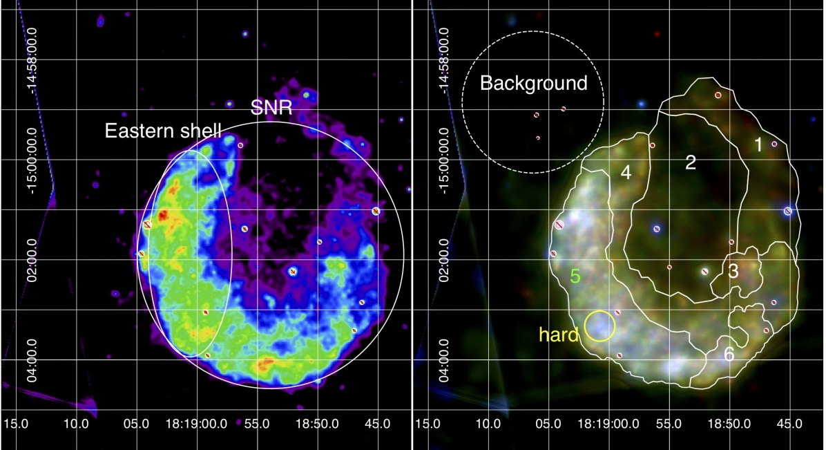
Figure 1: Broad-band mosaic X-ray image (0.3 – 8.0 keV) of SNR G15.9+0.2 taken with Chandra ACIS-S (left) and three-colour image (red = 1.0 – 2.0 keV, green = 2.0 – 3.5 keV, and blue = 3.5 – 7.0 keV, right). Regions used for the extraction of spectra are also shown. Point sources, visible in these images, were removed when the spectra were extracted. The images are all shown in equatorial coordinates. North is up, west is to the right.

2.2 H$\alpha$ image

To study the distribution of the colder ISM at the position of the SNR and verify whether the SNR has developed radiative filaments, we obtained H$\alpha$ and short red continuum images of the SuperCOSMOS H$\alpha$ survey (SHS, Parker et al., 2005), carried out by the Wide Field Astronomy Unit of the Institute for Astronomy of the Royal Observatory, Edinburgh. The continuum-subtracted H$\alpha$ image is shown in Fig. 2 (top left) with contours from the Chandra mosaic broad band image. No obvious H$\alpha$ emission related to the SNR can be found, which would have been a sign for the SNR being radiative. The image rather shows the distribution of warm gas on the line of sight. The H$\alpha$ emission is less bright on the eastern side (on the left-hand side in Fig. 2), indicating that material located on the line of sight is absorbing the background emission. As will be shown in Sect. 3, the X-ray emission of the SNR indicates higher absorption in this region, confirming that there is material located in front of the SNR.

2.3 Infrared

The SNR G15.9+0.2 has also been detected in the IR and shows a clearly shell-like structure similar to its morphology in X-rays. We have obtained the Spitzer InfraRed Array Camera (IRAC; Fazio et al., 2004) and Multiband Imaging Photometer (MIPS; Rieke et al., 2004) images from the Spitzer Heritage Archive. The IRAC images taken in October 2004 (program ID: 146) are a part of the GLIMPSE legacy survey (Benjamin et al., 2003; Churchwell et al., 2009), and the MIPS images were taken in September 2005 (program ID: 20597) as a part of the MIPSGAL survey (Carey et al., 2009). The pipeline-processed post-BCD images have been calibrated and mosaicked using pipelines S18.25 and S18.12 for IRAC and MIPS, respectively, and they are in units MJy/sr. The estimated flux calibration uncertainty for the pipeline products is 4 %.

We also extracted level 2.5 Herschel images taken with the Photodetector Array Camera (PACS; Poglitsch et al., 2010) and with the Spectral and Photometric Imaging Receiver (SPIRE; Griffin et al., 2010) from the Herschel Science Archive (OBSIDs 1342218997, 1342218998). The PACS images were taken at bands 70 and 160 $\mu$m and the SPIRE images at bands 250, 350, and 500 $\mu$m. The PACS 160 and SPIRE 350 $\mu$m images are shown in Fig. 2 (bottom). The observations were performed in April 2011 as a part of the Hi-GAL survey (Molinari et al., 2010). The Herschel 70 $\mu$m images were used in this work instead of the Spitzer 70 $\mu$m images because the spatial resolution of the PACS images is higher (5$\aas@@fstack{\prime\prime}$2 vs. 16″). The PACS images are in Jy/px format, and the extracted SPIRE images have been HiRes-processed (Xu et al., 2014). The absolute flux calibration error in PACS images is estimated to be 5 %.

SNR G15.9+0.2 is very clearly seen at 24 $\mu$m and 70 $\mu$m with a shell-like structure similar to the X-ray emission. The Spitzer MIPS 24 $\mu$m image shows the structure of the SNR best (see Fig. 2, middle left). At 24 $\mu$m the southern and eastern parts of the shell are bright, while at 70 $\mu$m the eastern side is bright. The IR emission of the SNR is well correlated with the X-ray emission, being bright in the east and in the south, whereas there seems to be little emission from the SNR to the northwest.

Emission from the SNR can be seen neither at shorter wavelengths (IRAC 3.6, 4.5, and 5.8 $\mu$m) nor at longer wavelengths (Herschel PACS 160 $\mu$m and SPIRE 250 $\mu$m, 350 $\mu$m, and 500 $\mu$m). In all Spitzer IRAC images at $\leq$8 $\mu$m two dark absorption features can be identified against the bright background at the eastern rim of the SNR shell and northeast of the center of the SNR (see Fig. 2, top right). These are most likely caused by dense foreground clouds. At 160 $\mu$m, 250 $\mu$m, and 350 $\mu$m some structures are seen in the SNR region but these are most likely not associated to the SNR itself. A bright spot is seen at longer wavelengths (Fig. 2, bottom), which seems to be associated with a foreground cloud.

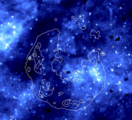
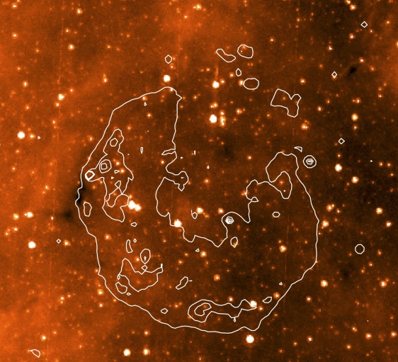
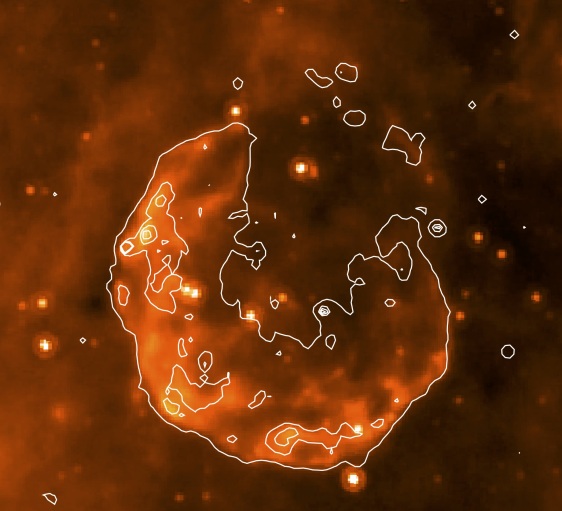
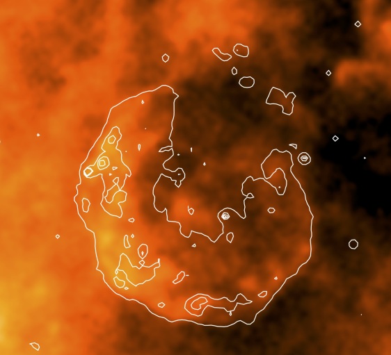
Figure 2: Top: SHS H$\alpha$ image (continuum-subtracted, left) and Spitzer IRAC 8.0 $\mu$m image (right). Middle: Spitzer MIPS 24 $\mu$m (left) and Herschel PACS 70 $\mu$m images (right), in which the SNR is well visible. Bottom: Herschel PACS 160 $\mu$m (left) and SPIRE 350 $\mu$m images (right). All images are presented in linear scale. The white contours are Chandra count rates from 2$\times 10^{-8}$ cts s^-1 to 2$\times 10^{-7}$ cts s^-1 in steps of 6$\times 10^{-8}$ cts s^-1.

3 Spectral analysis of X-ray data

Table 2: Best-fit parameters of the analysis of Chandra spectra. For the ellipse region in the bright shell see Table 3.

Region	$N_{\rm H}$	$kT$	Mg∗	Si∗	S∗	Ar∗	Ca∗	Fe∗	$\tau^{\triangledown}$	$norm$	$\chi^{2}$	d.o.f
	[cm-2]	[keV]	(solar)	(solar)	(solar)	(solar)	(solar)	(solar)	[s cm-3]	[cm-5]
VNEI
SNR⋆	3.5${}^{+0.2}_{-0.2}$e+22	1.1${}^{+0.1}_{-0.1}$	0.7${}^{+0.3}_{-0.1}$	0.9${}^{+0.1}_{-0.1}$	1.3${}^{+0.2}_{-0.1}$	1.3${}^{+0.2}_{-0.2}$	1.6${}^{+0.6}_{-0.7}$	0.3${}^{+0.3}_{-0.3}$	5.6${}^{+0.7}_{-0.4}$e+10	4.2${}^{+0.4}_{-0.6}$e–2	1.21	311
1	3.1${}^{+0.2}_{-0.3}$e+22	1.0${}^{+0.2}_{-0.2}$	-	-	-	-	-	-	6.0${}^{+5.1}_{-2.6}$e+10	2.1${}^{+0.9}_{-0.7}$e–3	0.87	182
2	3.2${}^{+0.4}_{-0.3}$e+22	1.0${}^{+0.3}_{-0.3}$	-	-	-	-	-	-	7.5${}^{+15.2}_{-3.3}$e+10	2.6${}^{+0.9}_{-0.7}$e–3	0.97	227
3	2.1${}^{+0.6}_{-0.5}$e+22	1.4${}^{+0.5}_{-0.3}$	-	-	-	-	-	-	3.7${}^{+3.1}_{-1.4}$e+10	5.0${}^{+3.5}_{-1.8}$e–4	1.13	83
4	3.7${}^{+0.1}_{-0.2}$e+22	1.0${}^{+0.1}_{-0.1}$	-	-	1.3${}^{+0.1}_{-0.2}$	-	-	-	9.0${}^{+2.6}_{-2.0}$e+10	1.1${}^{+0.2}_{-0.2}$e–2	1 17	251
5	4.1${}^{+0.1}_{-0.1}$e+22	1.1${}^{+0.1}_{-0.1}$	-	1.2${}^{+0.1}_{-0.1}$	1.6${}^{+0.1}_{-0.1}$	1.6${}^{+0.3}_{-0.2}$	-	-	6.4${}^{+0.5}_{-0.7}$e+10	2.6${}^{+0.3}_{-0.3}$e–2	1.17	233
6	3.3${}^{+0.2}_{-0.2}$e+22	1.1${}^{+0.1}_{-0.2}$	-	-	1.5${}^{+0.3}_{-0.2}$	2.0${}^{+0.8}_{-0.8}$	-	-	7.8${}^{+3.4}_{-1.9}$e+10	2.9${}^{+0.7}_{-0.5}$e–3	0.91	157
hard	4.4${}^{+0.4}_{-0.4}$e+22	1.4${}^{+0.4}_{-0.3}$	1.7${}^{+1.3}_{-0.9}$	1.7${}^{+0.5}_{-0.4}$	1.6${}^{+0.5}_{-0.4}$	-	-	-	6.1${}^{+2.4}_{-1.5}$e+10	1.1${}^{+0.6}_{-0.3}$e–3	1.01	100
VPSHOCK
SNR⋆	3.5${}^{+0.2}_{-0.3}$e+22	1.1${}^{+0.1}_{-0.1}$	0.8${}^{+0.2}_{-0.2}$	0.9${}^{+0.1}_{-0.1}$	1.6${}^{+0.1}_{-0.1}$	1.5${}^{+0.3}_{-0.1}$	1.7${}^{+0.6}_{-0.7}$	0.3${}^{+0.4}_{-0.2}$	1.1${}^{+0.1}_{-0.2}$e+11	4.3${}^{+0.5}_{-0.6}$e–2	1.25	311
5	4.1${}^{+0.1}_{-0.1}$e+22	1.1${}^{+0.1}_{-0.1}$	-	1.2${}^{+0.1}_{-0.1}$	1.8${}^{+0.1}_{-0.1}$	1.9${}^{+0.4}_{-0.3}$	-	-	1.1${}^{+0.2}_{-0.2}$e+11	2.9${}^{+0.1}_{-0.2}$e–2	1.32	232

^∗ For the sub-regions 1 to 6, and for the circular region around the hard emission, the abundances were fixed to 1.0 if they were consistent with solar values after they had been freed.
^▽ Upper limit of the ionisation timescale for the VPSHOCK model.
^⋆ Entire SNR.

For the analysis of the spectrum taken in X-rays, we extracted spectra from the newest Chandra data with the longest exposure time (ObsID 16766). Point sources have been removed from the data. We have tried different extraction regions based on X-ray and IR emission and have defined areas, which show similar spectral properties in X-rays based on preliminary spectral analyses. By this method we make sure that regions that have similar spectral properties in X-rays and coinciding brightness distribution between X-rays and IR are selected. At the same time the size of the regions should be not too small to have high enough statistics. The final extraction regions which have been used for the spectral analysis reported here are shown in Fig. 1. We analysed the spectra using the X-ray spectral fitting package XSPEC Ver. 12.8.2. All regions were analysed using the model VNEI, which reproduces the emission of a non-equilibrium ionisation (NEI) collisional plasma with variable element abundances. The spectrum of the entire SNR (in circular region shown in Fig. 1, left) has also been studied using the model VPSHOCK (emission from a plane-parallel shock with a range of ionisation timescale). The parameters of the best fits are listed in Table 2.

The fits of the entire SNR with VNEI and VPSHOCK models yield parameter values that are consistent with each other (Table 2, first and last rows). The average foreground column density is $N_{\rm H}$ = 3.5 $\times 10^{22}$ cm^-2 and the plasma temperature is $kT$ = 1.1 keV. Most of the elements have solar abundances, only S and Ar yield significantly higher values. The ionisation timescale is of the order of $\tau=nt=10^{11}$ s cm^-3, suggesting NEI. The absorbed X-ray flux of the SNR is $F_{\rm abs}(0.3-10.0\mathrm{~{}keV})=5.76\times 10^{-12}$ erg cm^-2 s^-1, whereas the unabsorbed flux is $F_{\rm unabs}(0.3-10.0\mathrm{~{}keV})=3.15\times 10^{-10}$ erg cm^-2 s^-1. The spectrum is shown in Fig. 3 (middle).

Due to lower statistics, the regions 1 - 6 have only been analysed using the VNEI model. The spectra of all six regions can be well fitted with a temperature that is consistent for all regions (and for the fit of the entire SNR). Also the ionisation timescale is consistent with each other. Region 3, which is the interior region showing rather soft emission (appearing red in Fig. 1, left), has lower foreground $N_{\rm H}$ than the other regions. Significantly higher $N_{\rm H}$ is obtained for the eastern shell (region 5), indicating that there is material on the line of sight. This is consistent with the distribution of H$\alpha$ emission, which shows absorption in the same region (Fig. 2, top left). In particular, there seems to be a dense cloud in front of the SNR at its eastern rim, seen as a dark absorption feature in the 8.0$\mu$ image (Fig. 2, top right). All regions can be nicely fitted with solar abundances for all elements. Only in regions 4, 5, and 6, freeing the parameter for S abundance and Ar abundance in regions 5 and 6 slightly improves the fits.

The results of the spectral analysis so far show that the X-ray emission of the SNR is dominated by that of shocked ISM and there is no significant spectral variation inside the SNR. However, there is a small region in the southeastern shell indicated with a yellow circle in the X-ray three-colour-image (Fig. 1, right), in which both the X-ray emission and the IR emission shows an interior arc-like structure. Moreover, this region appears blue in the X-ray three-colour image and thus seems to show harder X-ray emission. Therefore, we also extracted spectrum from this particular region in order to find out what the origin of the bright hard X-ray emission might be. The spectrum can be fitted well with a VNEI model with free abundances for Mg, Si, and S (see Table 2). These three elements turn out to be slightly overabundant. If one looks at the spectrum there is also a hint of excess at the position of the Fe K line, however, the statistics are too low to yield any significant fit parameter for the Fe abundance. Since this X-ray bright region is not bright in IR and the spectrum indicates overabundance of $\alpha$ elements, there might be a clump of heated ejecta at this position. The high foreground absorption does not allow us to determine abundances for O or Ne. We also looked for a non-thermal component in the spectrum. Adding a power-law component did not improve the fit but resulted in rather unrealistic values for the power-law index. Therefore, we conclude that the emission is fully thermal.

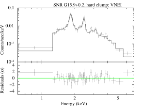
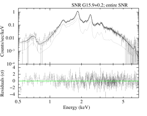
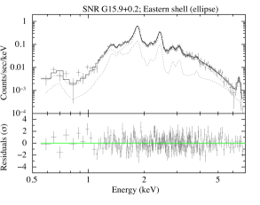
Figure 3: Chandra ACIS-S3 (ObsID: 16766) spectrum of the small blue-ish (‘hard’) region with the VNEI model (top), the entire SNR G15.9+0.2 with the best fit model (see Sect. 3.1, middle), and the ellipse region in the bright eastern shell (bottom). The fitted models and the residuals are also shown.

3.1 Ejecta emission

Our spectral parameters $N_{\rm H}$, $kT$, and $\tau$ are consistent with the results obtained by Maggi & Acero (2017). They also find a slight overabundance of elements Mg, Si, S, Ar, and Ca in various regions of the SNR. In addition, an excess at the position of the Fe K line at $\sim 6.5$ keV was found in the spectrum of the eastern part of the SNR shell. The Chandra spectra of the regions studied so far are all consistent with ISM abundance for Fe or indicate a lower Fe abundance. It is difficult to constrain the Fe abundance parameter since the spectrum is heavily absorbed below 1 keV where the Fe L emission would be observable.

In order to search for ejecta emission discovered by Maggi & Acero (2017) in the XMM-Newton spectrum, we extracted the spectrum of a larger region in the brighter eastern shell as indicated by the ellipse in Fig. 1 (left). As can be seen in the spectrum shown in Fig. 3 (bottom), there is a clear feature at 6.5 keV which is likely Fe K line emission. While this line was not significant in the spectrum of the entire SNR (see Fig. 3, middle), which also includes large portions with very faint emission, the source emission is bright enough with respect to the local X-ray background in the ellipse region to make the Fe K line detectable. We thus confirm the emission detected by Maggi & Acero (2017) and are able to study the ejecta emission using the spectrum of the bright eastern shell.

Table 3: Spectral fit results of the ellipse region in the bright shell.

Parameters	Model 1	Model 2
$N_{\rm H}$ [cm-2]	3.9${}^{+0.1}_{-0.1}$e+22	3.8${}^{+0.1}_{-0.1}$e+22
$kT_{\rm NEI}$ [keV]	1.0${}^{+0.1}_{-0.2}$	0.9${}^{+0.1}_{-0.1}$
$\tau_{\rm NEI}$ [s cm-3]	7.6${}^{+0.6}_{-0.6}$e+10	1.0${}^{+0.6}_{-0.3}$e+11
$norm_{\rm NEI}$ [cm-5]	3.2${}^{+0.3}_{-0.3}$e–2	3.9${}^{+0.4}_{-0.3}$e–2
$kT_{\rm VNEI}$ [keV]		3.0${}^{+0.7}_{-0.7}$
MgVNEI		34†
SiVNEI		8†
SVNEI		9†
ArVNEI		5†
CaVNEI		5†
FeVNEI		14†
$\tau_{\rm VNEI}$ [s cm-3]		2.6${}^{+0.9}_{-0.5}$e+10
$norm_{\rm VNEI}$ [cm-5]		6.3${}^{+2.3}_{-2.4}$e–4
$\chi^{2}$	1.8	1.0
d.o.f	220	216

^† Not well constrained (see text).

We first fitted the spectrum only assuming one NEI component with solar abundances. The best-fit parameters (see Table 3, Model 1) are similar to that of other shell regions (Table 2), but the reduced $\chi^{2}$ = 1.8 (with degrees of freedom d.o.f = 220) is high. We have therefore included an additional thermal component to model the ejecta emission, while the first component is used to model the ISM emission. For this additional ejecta component, we first set all element abundances to zero and fit the abundances of the elements Mg, Si, S, Ar, Ca, and Fe by freeing the parameters one by one. The abundances of these elements become significantly higher than solar. The fit results of the initial NEI component with solar abundances for all elements, are $kT=0.89~{}(+0.03,-0.05)$ keV and $\tau=1.0~{}(+0.6,-0.3)\times 10^{11}$ s cm^-3. The best fit has a reduced $\chi^{2}$ of 1.0 for 216 degrees of freedom (see Table 3, Model 2). Since the normalisation and the element abundances are strongly dependent on each other, the parameters of the second component are not well constrained. The fitted values relative to solar abundances are Mg:Si:S:Ar:Ca:Fe = 34:8:9:5:5:14. The best fit absorbing column density for the whole model is $N_{\rm H}$ = $3.8~{}(+0.1,-0.1)\times 10^{22}$ cm^-2. This yields an absorbed X-ray flux for the ISM component of the eastern (E) shell of $F_{\rm abs,ISM,E}(0.3-10.0\mathrm{~{}keV})=4.5\times 10^{-12}$ erg cm^-2 s^-1, and for the ejecta component $F_{\rm abs,ejecta,E}(0.3-10.0\mathrm{~{}keV})=1.3\times 10^{-12}$ erg cm^-2 s^-1.

As shown before, the ejecta component is not detected significantly in the spectrum of the entire SNR. However, in order to get an estimate of the emission components in the entire SNR, we freeze all parameters of the two additive spectral components except for the normalisations and use the model for the fit of the spectrum of the SNR. We thus keep the shape of the spectral components but rescale their fluxes. This method yields a spectral fit with a reduced $\chi^{2}$ of 1.1 for 315 degrees of freedom. For the SNR, we obtain an absorbed X-ray flux for the ISM component of $F_{\rm abs,ISM}(0.3-10.0\mathrm{~{}keV})=4.3\times 10^{-12}$ erg cm^-2 s^-1, and for the ejecta component $F_{\rm abs,ejecta}(0.3-10.0\mathrm{~{}keV})=1.6\times 10^{-12}$ erg cm^-2 s^-1. The spectra with the best-fit models are shown in Fig. 3 (middle and bottom).

4 Infrared fluxes

To study the IR emission from the SNR, we measured the SNR flux densities in an aperture with a radius of 160″ and estimated the local background in a region located south of the SNR. The background region was selected to have low IR surface brightness and exclude any prominent IR features. The other directions outside the SNR contain external emission in the southeast direction, SNR dust in the north and an apparent brighter edge of a cloud in the northeast direction (“NE rim”). Therefore, we did not use an annulus around the source aperture to estimate the background. Point sources were masked in the IRAC 8.0 and 24 $\mu$m images. The Herschel images do not contain point sources. The dark absorption cores seen at 8.0 and 24 $\mu$m are masked out, and their emission counterparts in the Herschel images are also masked (these features include the foreground clump in the northwest of the SNR center and the eastern rim clumps) if they are seen in the images. Furthermore, at 8 $\mu$m image artefacts ("jailbars") were masked. The median value of the sky brightness was used as the background value. The background-subtracted aperture flux density was then converted into Janskys.

The measured flux densities were aperture-corrected, but not colour- or extinction-corrected. Omitting the colour-correction will produce typically an error from a few to 10 % percent. The flux density values for the SNR are $3.2\pm 1.5$, $15.9\pm 4.0$, and $88.5\pm 9.5$ Jy for 8.0, 24, and 70 $\mu$m, respectively. The SNR G15.9+0.2 IR flux densities have been previously computed as a part of larger SNR surveys. Pinheiro Gonçalves et al. (2011) obtained aperture-corrected values at 8.0, 24, and 70 $\mu$m of $3.2\pm 2.5$, $16\pm 2$, and $55\pm 16$ Jy, respectively, using Spitzer data. Koo et al. (2016) used Spitzer MIPS 24 $\mu$m and Herschel PACS 70 $\mu$m observations to derive fluxes of $10.1\pm 0.4$ and $49.1\pm 2.7$ Jy, respectively.

In addition to the SNR, we had inspected the exterior NE rim properties to verify whether the region could be used for extracting the background value for the SNR. We compared the surface brightnesses in the NE rim and the chosen background region. For this no background value was subtracted of either region. The results are listed in Table 4. At all observed wavelengths the surface brightness in the background region is lower. Comparing the IR images with the H$\alpha$ image suggests that the NE rim is the brightened edge of the large foreground cloud seen in H$\alpha$. This together with the surface brightness values suggests that the NE rim is an object separate from the SNR. The derived background-subtracted flux densities for NE rim are $1.7\pm 1.3$, $1.2\pm 1.1$, $15.1\pm 3.9$, and $51.3\pm 7.2$ Jy, at 8, 24, 70, and 160 $\mu$m, respectively. These are not aperture-corrected, and the corrections introduce at the most a $\sim$10% error.

Table 4: Comparison of surface brightness in the NE rim and the background regions.

Wavelength	Background	NE rim
$[\mu\mathrm{m}]$	[MJy/sr]	[MJy/sr]
8	59.7	69.8
24	70.3	77.4
70	7.0	93.7
160	409.2	700.9

5 Discussion

5.1 SNR properties assuming Sedov solution

The morphology and the X-ray spectrum of SNR G15.9+0.2, which is consistent with ISM emission, indicate that it is in the Sedov phase. Therefore, we calculate its physical parameters using the Sedov-Taylor-von Neumann similarity solution (Sedov, 1959; Taylor, 1950; von Neumann, 1947). For cosmic abundances (Anders & Grevesse, 1989), the gas density is $n_{\rm gas}=1.1~{}n_{\rm H}$, where $n_{\rm H}$ is the atomic H number density. For fully ionised plasma which can be expected for an X-ray SNR, the electron number density is for cosmic abundances is $n_{\rm e}=1.21~{}n_{\rm H}$. Therefore, the total number density of the gas is $n=n_{\rm e}+n_{\rm i}=2.3~{}n_{\rm H}$ with a mean mass per free particle $\bar{m}=0.61~{}m_{\rm p}$, with proton mass $m_{\rm p}$. We estimate the shock velocity using the mean shock temperature $kT$ = 0.89 $\pm$ 0.05 keV for the ISM component obtained from the fit of the ellipse region in the eastern shell as well as the entire SNR assuming ISM and ejecta components. With

$$v_{\rm s}=\left(\frac{16kT_{\rm s}}{3\bar{m}}\right)^{1/2},$$ (1)

where $k$ is the Boltzmann’s constant, the shock velocity is $v_{\rm s}$ = 860 $\pm$ 30 km s^-1.

If we ignore the northern blow-out, the SNR can be regarded as a nicely circular shell with a radius of $\theta$ = 155″$\pm$ 5″= $(7.5\pm 0.3)\times 10^{-4}$ rad as can be verified in the deep Chandra mosaic image (see Fig. 1, right). The linear radius can be written as $R_{\rm s}=(7.5\pm 0.3)\times d_{\rm 10kpc}$ pc or $R_{\rm s}=(2.3\pm 0.1)\times 10^{19}\times d_{\rm 10kpc}$ cm with $d_{\rm 10kpc}$ being the distance normalised to 10 kpc. Unfortunately, the distance $d$ to SNR G15.9+0.2 is not yet known. Caswell et al. (1982) obtained a distance of 16.7 kpc based on a $\Sigma$-$D$-relation, which would result in a rather unrealistic large size with a diameter of 27 pc. High foreground absorption indicates that the SNR is most likely located close to or on the other side of the Galactic center. Therefore, Reynolds et al. (2006) used a fiducial distance of 8.5 kpc in their calculations. We thus have $d_{\rm 10kpc}=0.85-1.67$. The age of the remnant can be estimated from the shock velocity using the Sedov similarity solution:

$$t=\frac{2R_{\rm s}}{5v_{\rm s}}$$ (2)

yielding an age estimate of $t$ = $(1.1\pm 0.1)\times 10^{11}d_{\rm 10kpc}$ s = $(3400\pm 200)\times d_{\rm 10kpc}$ yr.

From the normalisation of the NEI or the VNEI, which is defined as $norm=10^{-14}/(4\pi d^{2})\times\int n_{\rm e}n_{\rm H}dV$ [cm^-5], one can estimate the densities. We rearrange the integral $\int n_{\rm e}n_{\rm H}dV$ using $n_{\rm e}=(n_{\rm e}/n_{\rm H})n_{\rm H}$ and $n_{\rm e}/n_{\rm H}=1.21=const$ into $(n_{\rm e}/n_{\rm H})\int n_{\rm H}^{2}dV=(n_{\rm e}/n_{\rm H})\int_{0}^{R_{\rm s}}4\pi R^{2}n_{\rm H}^{2}dR=(n_{\rm e}/n_{\rm H})2.06n_{\rm H,0}^{2}(4/3)\pi R_{\rm s}^{3}$. For the integration in the last step, the calculation by Kahn (1975) for the Sedov solution has been used (see, e.g., Cox & Anderson, 1982). Therefore, we get $norm$ $=8.3\times 10^{-15}n_{\rm H,0}^{2}R_{\rm s}^{3}d^{-2}$. Using the normalisation obtained for the ISM component of the spectrum of the entire SNR, the initial H density is $n_{\rm H,0}=3.0\times(norm/d_{\rm 10kpc})^{1/2}=(0.73\pm 0.06)\times d_{\rm 10kpc}^{-1/2}$ cm^-3 and the gas density is $n_{\rm gas,0}=1.1n_{\rm H,0}=(0.81\pm 0.06)\times d_{\rm 10kpc}^{-1/2}$ cm^-3. If we assume that this is the mean number density of the interstellar gas in which the SNR is expanding, the mass of ISM that the SNR has shocked is $M_{\rm ISM}=4\pi/3R_{\rm s}^{3}\times 1.4n_{\rm H,0}m_{\rm p}=44M_{\sun}\times d_{\rm 10kpc}^{2.5}$.

For a distance in the range of $d$ = 8.5 – 16.7 kpc, the SNR age and the ambient H density are $t$ = (2900 $\pm$ 200) – (5700 $\pm$ 300) yr and $n_{\rm H,0}$ = (0.79 $\pm$ 0.07) – (0.56 $\pm$ 0.05) cm^-3, respectively. These numbers are realistic for both extreme values of the distance and do not allow us to constrain the distance.

The circular morphology of the SNR and the distribution of the cold ISM as seen in the IR images suggest that the SNR is expanding in a region with a higher density in the south and the east and lower density in particular in the northwest. Therefore, the outer shock could expand further in the northwest than in the rest of the SNR. On this lower-density side of the ISM, the evolution of the SNR is not significantly affected by the existence of higher-density gas on the other side. Therefore, one can apply the Sedov solution also for this part of the SNR. The distance of the outer rim in the north from the geometrical center of the circle around the bright main part of SNR G15.9+0.2 is $\theta_{\mathrm{n}}$ = 210″$\pm$ 10″, corresponding to $R_{\rm s,n}=(10.2\pm 0.5)\times d_{\rm 10kpc}$ pc $=(3.1\pm 0.1)\times 10^{19}\times d_{\rm 10kpc}$ cm. If we now use the age which was derived from the rest of the remnant we can calculate the expansion velocity and the ambient density based on the Sedov solution: $v_{\rm s,n}=2R_{\rm s,n}/(5t)$ = $1100\pm 100$ km s^-1. Since for the Sedov solution, we have the relation: $R_{\rm s}\propto n_{\rm gas,0}^{-1/5}t^{2/5}$, and the age $t$ is obviously the same for the northern part and for the rest of the SNR, one gets: $n_{\rm gas,0,n}=R_{\rm s}^{5}/R_{\rm s,n}^{5}n_{\rm gas,0}$ = $(0.18\pm 0.02)\times d_{\rm 10kpc}^{-1/2}$ cm^-3. Therefore, there is a change in ambient density of a factor of $\sim$4.6 in $\sim$20 pc, which allowed the shock to propagate faster in the north. In principle, this difference in velocity should also be observable in the spectrum of the thermal X-ray emission, which should have a higher temperature. However, the very low statistics in the northern blow-out region makes it not possible to measure the temperature of the emitting plasma. On the other hand, the interaction of the SNR with the denser ISM in the south and in the east resulted in higher emissivity and thus brighter X-ray emission. Furthermore, the shocks also caused the heating of dust on this side, which makes the SNR detectable also in IR at 24 $\mu$m and 70 $\mu$m.

So far, not many SNRs with CCOs have been found. Since the morphology and the evolution of an SNR strongly depend on the geometry of the progenitor and the circumstellar/interstellar environments in which it is located, the study of SNRs are crucial for a better understanding of the formation mechanisms of different types of neutron stars. The most famous SNR with a CCO with an age which is about one order of magnitude lower is SNR Cas A. For Cas A an age of $\sim$320 yr (Ashworth, 1980; Fesen et al., 2006) and a shock velocity of 5200 km s^-1 was measured. A major difference between SNR G15.9+0.2 and Cas A is that the reverse shock is still in the process of heating the ejecta and is observable in Cas A (Gotthelf et al., 2001; Morse et al., 2004) and that its outer shock has traveled through the circumstellar medium not too long ago, while SNR G15.9+0.2  is well in the Sedov phase. Arendt et al. (2014) derived a mass of 0.04$M_{\sun}$ for the shocked hot component of the dust inside Cas A, while the still unaffected cold dust component in the unshocked ejecta is estimated to be $\mathrel{\hbox{\hbox to0.0pt{\hbox{\lower 4.0pt\hbox{$\sim$}}\hss}\hbox{$<$}}}$0.1$M_{\sun}$.

5.2 Ejecta mass

In Section 3.1 we showed that the X-ray spectrum of the entire SNR can be fit well with a model consisting of a solar-abundance ISM component and an ejecta component with higher abundances for elements Mg, Si, S, Ar, Ca, and Fe. Assuming a homogeneous density for ejecta, we can estimate the ejecta mass from the spectral parameters. We use the the normalisation parameter of the ejecta component of the spectrum of the entire SNR, which is $norm=2.1(-0.6,+1.6)\times 10^{-3}$ cm^-5. Using the assumed solar abundance values for the spectral fit (Anders & Grevesse, 1989) and the fitted abundance values relative to solar, we obtain $M_{\text{Mg}}$ = 0.0536 $\times d_{\rm 10kpc}^{2}M_{\sun}$, $M_{\text{Si}}$ = 0.0139 $\times d_{\rm 10kpc}^{2}M_{\sun}$, $M_{\text{S}}$ = 0.00828 $\times d_{\rm 10kpc}^{2}M_{\sun}$, $M_{\text{Ar}}$ = 0.00135 $\times d_{\rm 10kpc}^{2}M_{\sun}$, $M_{\text{Ca}}$ = 0.000709 $\times d_{\rm 10kpc}^{2}M_{\sun}$, and $M_{\text{Fe}}$ = 0.0632 $\times d_{\rm 10kpc}^{2}M_{\sun}$ for the part of the ejecta, which has been ionised and heated by the reverse shock. These values have large uncertainties, since the abundance parameters together with the $norm$ parameter are not well constrained. The comparison to the nucleosynthesis yields for core-collapse SNe presented by Nomoto et al. (1997) shows that the estimated masses and abundance ratios suggest a progenitor mass of $\mathrel{\hbox{\hbox to0.0pt{\hbox{\lower 4.0pt\hbox{$\sim$}}\hss}\hbox{$<$}}}20~{}M_{\sun}$.

5.3 Dust properties

We derive the dust temperature $T_{\rm d}$ from the IR flux ratios. We assume that the emission comes mainly from shocked hot dust that can be described with a single temperature $T_{\rm d}$ and a modified black-body emission:

$$F_{\nu}\propto\nu^{\beta}B_{\nu}(T_{\rm d})$$ (3)

where $F_{\nu}$ is the flux density, $\beta$ is the dust emissivity index which depends on the dust composition ($\beta\sim 1-2$, we use $\beta=2$), and $B_{\nu}(T_{\rm d})$ is the Planck function evaluated at $T_{\rm d}$. Following this we can solve $T_{\rm d}$ from the ratio

$$\frac{F_{\nu_{1}}}{F_{\nu_{2}}}=\left(\frac{\nu_{1}}{\nu_{2}}\right)^{\beta}\frac{B_{\nu_{1}}(T_{d})}{B_{\nu_{2}}(T_{\rm d})}.$$ (4)

Using the measured flux densities for 24 and 70 $\mu$m (Sect. 4) we get 55.9 K. Pinheiro Gonçalves et al. (2011) obtained 60 K, and Koo et al. (2016) 57.8 K using the same ratio $F_{24}/F_{70}$.

For the outside NE rim, the flux density ratios $F_{24}/F_{70}$ and $F_{70}/F_{160}$ yield temperatures of 50.3 K and 21.6 K, respectively. The flux density at 24 $\mu$m is very low and has relatively high errors, but within the $F_{24}$ 1-$\sigma$ error the derived temperature is lower than the one derived for the SNR. For the SNR dust we cannot derive a flux density value at 160 $\mu$m as there is no discernible emission from the SNR. We can however measure the emission at 160 $\mu$m and use the error to estimate an upper limit for the flux density of the SNR dust. The 3-$\sigma$ upper limit for the flux density $F_{160}$ is 35.1 Jy. Using the $F_{160}$ upper limit, the ratio $F_{70}/F_{160}$ corresponds to a temperature of 37.1 K for the SNR. Flux densities lower than the $F_{160}$ upper limit would result in even higher temperature values. This suggests that the dust at the NE rim is colder than the SNR dust.

The total IR flux $F_{\rm IR}$ can be estimated using

$$\frac{F_{\rm IR}}{\nu F_{70}}=\frac{\int\kappa_{\nu}B_{\nu}(T_{\rm d})d\nu}{\nu\kappa_{\nu}B_{\nu}(T_{\rm d})}$$ (5)

where $\kappa_{\nu}$ is the mass absorption coefficient ($\kappa_{\nu}\propto\lambda^{-\beta}$). Koo et al. (2016) calculated $F_{\rm IR}=4.32\times 10^{-9}$ erg cm^-2 s^-1. Our values for $F_{70}$ and $T_{\rm d}$ give $F_{\rm IR}=7.21\times 10^{-9}$ erg cm^-2 s^-1.

If the observed IR emission is solely due to thermal dust emission, the SNR dust mass can be estimated using the following equation:

$$M_{\rm dust}=\frac{d^{2}F_{\nu}}{\kappa_{\nu}B_{\nu}(T_{\rm d})}$$ (6)

where $d$ is the distance to the SNR, and $\kappa_{\nu}$ the dust mass absorption coefficient. We evaluate the dust mass at 24 $\mu$m based on the derived temperature 55.9 K. For $\kappa_{\nu}$ we use the dust model by Draine (2003a, b) for a mixture of silicates and carbonaceous grains. At 24 $\mu$m the dust mass absorption coefficient is 505.9 cm${}^{2}\,$g^-1 which yields $M_{\rm dust}=0.24\times d_{\rm 10kpc}^{2}M_{\odot}=0.17-0.67M_{\odot}$ when $d_{\rm 10kpc}$ = 0.85 – 1.67. Pinheiro Gonçalves et al. (2011) derived a dust mass of 0.081 $M_{\odot}$ using a distance of 8.5 kpc.

We use the $N_{\rm H}$ derived from the X-ray modelling to estimate the extinction correction at 24 $\mu$m: $N_{\rm H}=3.5\times 10^{22}$ cm^-2 corresponds to $A_{V}=18.7$ mag and hence $A_{Ks}=2.1$ mag using the extinction law adapted from Cardelli et al. (1989) and $A_{\rm 24}=0.72$ mag (Chapman et al., 2009). The extinction-corrected flux density is then $1.96\times F_{24}$, leading to a derived dust temperature $T_{\rm d}=61.9$ K and a dust mass of $0.16\times d_{\rm 10kpc}^{2}M_{\odot}$. Using the shocked ISM mass of $M_{\rm ISM}=44M_{\sun}\times d_{\rm 10kpc}^{2.5}$, the dust-to-gas mass ratio is $M_{\rm dust}/M_{\rm ISM}=0.0036\times d_{\rm 10kpc}^{-0.5}=0.0028-0.0039$, a little less but still comparable to the average dust-to-gas mass ratio measured in the ISM of the Milky Way and nearby galaxies (Draine et al., 2007).

However, we note that the use of a single-temperature dust population in thermal equilibrium is a highly simplified view of the situation. Furthermore, even though the SNR is very young and not yet fully in the radiative phase, some of the observed IR flux can also be from line emission instead of thermal dust emission. This causes our dust mass estimate to be an upper limit.

5.4 IR-X comparison

The kinetic energy of the SNR shock is dissipated by interaction of charged particles and the electromagnetic fields and thus heat the plasma, and subsequently, the dust. The efficiency of converting the kinetic energy of the shock into IR radiation of dust $\epsilon_{\rm IR}$ can be estimated using the relation

$$\epsilon_{\rm IR}=L_{\rm IR}/\bigg{(}\frac{1}{2}n_{\rm H,0}\mu_{\rm H}v_{s}^{3}\times 4\pi R_{s}^{2}\bigg{)}$$ (7)

with $n_{\rm H,0}$ being the ambient density, $\mu_{\rm H}=1.4$ the mean relative mass per hydrogen atom, $v_{s}$ the SNR shock velocity, $R_{s}$ the SNR radius (Koo et al., 2016). If one compares the X-ray images (Fig. 1) with the IR image (Fig. 2) it is striking that the X-ray emission agrees well with structures in the IR shell. Using the parameters obtained from the new X-ray and IR analyses, we get for the IR conversion efficiency $\epsilon_{\rm IR}=0.024d_{\rm 10kpc}^{1/2}$. This value is one to two orders of magnitude lower than the value obtained by Koo et al. (2016) for well-known mixed-morphology SNRs. Compared to these SNRs, the morphology of which is believed to be due to shocked emission from shocked interstellar clouds, SNR G15.9+0.2 is younger and is expanding in a low-density medium.

6 Summary

We have studied the X-ray emission of SNR G15.9+0.2 using the newest Chandra data. The spectrum of the SNR is consistent with that of thermal emission from shocked ISM. In a smaller region in the shell we also found some enhancement of the silicon and sulfur abundances, which might indicate emission from an ejecta clump. The spectrum of the bright eastern part of the shell shows a clear Fe K line at $\sim$6.5 keV. This spectrum has been modelled with two thermal components, simulating shocked ISM and shocked ejecta. Using the same model components, we model the spectrum of the entire SNR. Based on a comparison with nucleosynthesis yields calculations, we estimate that the progenitor had a mass of $\mathrel{\hbox{\hbox to0.0pt{\hbox{\lower 4.0pt\hbox{$\sim$}}\hss}\hbox{$<$}}}$ 20 $M_{\odot}$. For the possible range for the distance of $d$ = 8.5 – 16.7 kpc, the parameters derived from the analysis of the X-ray emission yield reasonable values for the SNR age of $t$ = (2900 $\pm$ 200) – (5700 $\pm$ 300) yr and the H density of $n_{\rm H,0}$ = (0.79 $\pm$ 0.07) – (0.56 $\pm$ 0.05) cm^-3, not allowing to constrain the distance. The total mass of shocked ISM is $M_{\rm ISM}$ = (30 – 160) $M_{\sun}$.

To study the morphology of the SNR and its relation with the ambient ISM, we also used H$\alpha$ data from the SuperCOSMOS H$\alpha$ survey and infrared data of Herschel and Spitzer. These data at lower energies indicates that the SNR is located in a region with a complex distribution of colder gas and dust. There is a negative density gradient from southeast to northwest, which is responsible for the shape of the SNR which indicates a blow-out to the north. We derived a dust temperature and mass of $T_{\rm d}=61.9$ K and SNR dust mass 0.12 – 0.45 $M_{\odot}$, corresponding to a dust-to-gas mass ratio of $M_{\rm dust}/M_{\rm ISM}=0.0028-0.0039$. Based on IR flux and the shock parameters obtained from the X-ray analysis, we have shown that the shock-IR-conversion efficiency is low and suggest that, even though the morphologies in IR and X-ray match very well, only a small fraction of the energy has been used for the heating of dust.

References

- Anders & Grevesse (1989) Anders E., Grevesse N., 1989, Geochimica et Cosmochimica Acta, 53, 197
- Arendt et al. (2014) Arendt R. G., Dwek E., Kober G., Rho J., Hwang U., 2014, ApJ, 786, 55
- Ashworth (1980) Ashworth Jr. W. B., 1980, Journal for the History of Astronomy, 11, 1
- Benjamin et al. (2003) Benjamin R. A., et al., 2003, PASP, 115, 953
- Cardelli et al. (1989) Cardelli J. A., Clayton G. C., Mathis J. S., 1989, ApJ, 345, 245
- Carey et al. (2009) Carey S. J., et al., 2009, PASP, 121, 76
- Caswell et al. (1982) Caswell J. L., Haynes R. F., Milne D. K., Wellington K. J., 1982, MNRAS, 200, 1143
- Chapman et al. (2009) Chapman N. L., Mundy L. G., Lai S.-P., Evans II N. J., 2009, ApJ, 690, 496
- Churchwell et al. (2009) Churchwell E., et al., 2009, PASP, 121, 213
- Clark et al. (1975) Clark D. H., Caswell J. L., Green A. J., 1975, Australian Journal of Physics Astrophysical Supplement, 37, 1
- Cox & Anderson (1982) Cox D. P., Anderson P. R., 1982, ApJ, 253, 268
- De Looze et al. (2017) De Looze I., Barlow M. J., Swinyard B. M., Rho J., Gomez H. L., Matsuura M., Wesson R., 2017, MNRAS, 465, 3309
- Doroshenko et al. (2016) Doroshenko V., Pühlhofer G., Kavanagh P., Santangelo A., Suleimanov V., Klochkov D., 2016, MNRAS, 458, 2565
- Draine (2003a) Draine B. T., 2003a, ARA&A, 41, 241
- Draine (2003b) Draine B. T., 2003b, ApJ, 598, 1017
- Draine et al. (2007) Draine B. T., et al., 2007, ApJ, 663, 866
- Fazio et al. (2004) Fazio G. G., et al., 2004, ApJS, 154, 10
- Fesen et al. (2006) Fesen R. A., et al., 2006, ApJ, 645, 283
- Gotthelf et al. (2001) Gotthelf E. V., Koralesky B., Rudnick L., Jones T. W., Hwang U., Petre R., 2001, ApJ, 552, L39
- Griffin et al. (2010) Griffin M. J., et al., 2010, A&A, 518, L3
- Kahn (1975) Kahn F. D., 1975, International Cosmic Ray Conference, 11, 3566
- Klochkov et al. (2016) Klochkov D., Suleimanov V., Sasaki M., Santangelo A., 2016, A&A, 592, L12
- Koo et al. (2016) Koo B.-C., Lee J.-J., Jeong I.-G., Seok J. Y., Kim H.-J., 2016, ApJ, 821, 20
- Maggi & Acero (2017) Maggi P., Acero F., 2017, A&A, 597, A65
- Molinari et al. (2010) Molinari S., et al., 2010, PASP, 122, 314
- Morse et al. (2004) Morse J. A., Fesen R. A., Chevalier R. A., Borkowski K. J., Gerardy C. L., Lawrence S. S., van den Bergh S., 2004, ApJ, 614, 727
- Nomoto et al. (1997) Nomoto K., Hashimoto M., Tsujimoto T., Thielemann F.-K., Kishimoto N., Kubo Y., Nakasato N., 1997, Nuclear Physics A, 616, 79
- Parker et al. (2005) Parker Q. A., et al., 2005, MNRAS, 362, 689
- Pinheiro Gonçalves et al. (2011) Pinheiro Gonçalves D., Noriega-Crespo A., Paladini R., Martin P. G., Carey S. J., 2011, AJ, 142, 47
- Poglitsch et al. (2010) Poglitsch A., et al., 2010, A&A, 518, L2
- Reynolds et al. (2006) Reynolds S. P., Borkowski K. J., Hwang U., Harrus I., Petre R., Dubner G., 2006, ApJ, 652, L45
- Rieke et al. (2004) Rieke G. H., et al., 2004, ApJS, 154, 25
- Sedov (1959) Sedov L. I., 1959, Similarity and Dimensional Methods in Mechanics, Academic Press, New York
- Sun et al. (2011) Sun X. H., Reich P., Reich W., Xiao L., Gao X. Y., Han J. L., 2011, A&A, 536, A83
- Taylor (1950) Taylor G. I., 1950, Proc. R. Soc. London A, 201, 159
- Xu et al. (2014) Xu C. K., et al., 2014, preprint, (arXiv:1401.2109)
- von Neumann (1947) von Neumann J., 1947, Los Alamos Sci. Lab. Tech. Series, Vol. 7