Combining Radon transform and Electrical Capacitance Tomography for a $2d+1$ imaging device

Abstract

This paper describes a coplanar non invasive non destructive capacitive imaging device. We first introduce a mathematical model for its output, and discuss some of its theoretical capabilities. We show that the data obtained from this device can be interpreted as a weighted Radon transform of the electrical permittivity of the measured object near its surface. Image reconstructions from experimental data provide good surface resolution as well as short depth imaging, making the apparatus a $2d+1$ imager. The quality of the images leads us to expect that excellent results can be delivered by ad-hoc optimized inversion formulas. There are also interesting, yet unexplored, theoretical questions on imaging that this sensor will allow to test.

1 Introduction

The imaging capability of electrical capacity sensors – sometimes called dielectrometry – has been discussed in connection with applications to a variety of domains [19, 22, 25], from chemical engineering [21] to medical imaging [12]. It is very closely related to Electrical Impedance Tomography (EIT) in terms of the partial differential equation used in the associated quasi-static model [28, 7, 14, 27, 1]. Several features are nevertheless specific to this modality: in particular, physical contact is not required between the sample and the measurement device. Furthermore, measurements can be performed on one side only [20, 2, 19]. The design of electrodes for Electrical Capacitance Tomography (ECT) and EIT is different. Inter-digital, periodic, grating sensors or the multiplexing device described in this note are line sensors [19, 2, 22]: their output cannot be approximated as pointwise data. Volumetric capacitive measurements, using planar sensors of smaller diameter, have been discussed and analysed in many articles [25, 15, 29]. The purpose of these studies is to detect the presence of objects at a significant depth. Here the imaging device under consideration is focused on retrieving near-field details, rather than deep coarse features.

\begin{picture}(6897.0,3238.0)(1687.0,-3487.0)\end{picture}

Figure 1.1: Sketch of the imaging setup.

The imaging device under consideration is flat: it is represented schematically in 1.1, and physically in 1.4. It has been developed by Zedsen Limited. The dielectric material (a light blue Z, for illustration purposes) is held above the apparatus. The sensor is composed of a series of narrow electrodes [18], which can act as either receiver or transmitter. In 1.1, assuming that the leftmost (blue) electrode is the emitter, either the red, green, brown or magenta electrode is used as a receiver, while all others are grounded. The transmitting electrode sends a pulse for a short duration. The resulting voltage is measured on the receiving electrodes at several time steps. Thus, for a given grid of $2n+1$ electrodes, we obtain ${\color[rgb]{1,0,0}2n}+{\color[rgb]{0,1,0}2n-1}+{\color[rgb]{.75,.5,.25}2n-2}+{\color[rgb]{.75,0,.25}2n-3}$ measures, at a few time points. The imaging device is equipped with a second set of $2m+1$ electrodes placed orthogonally to the first set, leading to another $8m-6$ measurements. Cross measurements are also possible, e.g. transmitting from an horizontal electrode and measuring on a vertical one or vice-versa, leading to $\left(2n+1\right)\times\left(2m+1\right)$ measurements .

\begin{picture}(9001.0,6369.0)(147.0,-12448.0)\end{picture}

Figure 1.2: Schematic cross section, fringing field and capacitive network interpretations.

The rationale for such measurements is based on two dimensional problem reduction considerations. Consider a vertical cross-section of the problem as described in 1.2. If a long vertical homogeneous dielectric is placed on the sensor, the problem becomes approximately two dimensional, and the red, green, brown and magenta electrodes measure the output at an increasing distance. Modelling the system as an electric circuit, which can be justified for very contrasted materials (in the case of electrical impedance tomography, see [27, 8, 7]) this leads to the determination of up to $10$ capacitances. Alternatively, in the case of a weakly contrasted material, viewing the system as a perturbation of the free space, the fringing field zone of dependence – the area where the gradient of the electrostatic potential is large enough to have an effect – is often modelled as semi-discs. As the distance between the source and the receiver increases, the data collected by the sensor depends on the permittivity of deeper and deeper layers. Assuming that the medium is suitably homogeneous, other planar ECT sensors have been shown to provide some depth capacitive data, interdigital devices in particular [16, 11]; assuming that the electric field decays so fast that its amplitude is negligible after the fourth electrodes, similar heuristic approximations could be devised in this case as well.

There are limitations to this approach. An object placed diagonally provides the same output as a horizontal one with an adequate cross section, since the output are summed along lines: these data sets are linear in $n$ and $m$. The cross sectional measurements, from vertical to horizontal electrodes or vice-versa, do provide more localised information, with potentially $\left(2n+1\right)\times\left(2m+1\right)$ independent data points. However, depth dependent information is then only available, indirectly, by means of different time points. The theoretical framework to take advantage of such data is under-developed at this time, and preliminary computations in model cases tend to indicate that the dependence on time difference data could be logarithmic. Collating the localized horizontal data and vertical or horizontal depth measurements does not scale correctly (with respect to the interdigital distance) to provide multi-layered data, but for coarse horizontal grids. One feature of this sensor device is that its horizontal resolution, namely, the distance between the line electrodes, can be adapted to the application at hand. This makes it different from interdigital sensors, where the distance between the gratings determines a wavelength, which is of course related to a spatial resolution, but indirectly. To address these limitations, the dielectrometric imaging device has been mounted on a rotating support, as represented in 1.3 and pictured in 1.4.

\begin{picture}(7197.0,5764.0)(2931.0,-12673.0)\end{picture}

Figure 1.3: The sensor with rotational support.

The dielectric to be imaged is static, while the sensor array is placed on a turntable, rotating by with fixed angular increments of $\pi/p$ radians. As the data are non-directional, all non redundant data are collected after $p$ angular steps. All together, the data collected is an array of size $10p\times\left(\frac{2}{5}n\times m+n+m-1\right)$, for every time-point.

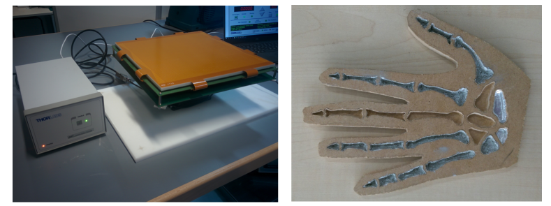
Figure 1.4: The hand model (Kenny’s) is approximately $200$mm long. The sensor array has $55\times 56$ sensor lines $d=2.5$mm apart, covering a $280\times 280$mm square. There were $36,90$ or 180 rotational increments ($1,2$ or $5$ degrees each time). The hand was suspended $2$mm above the sensor array, avoiding contact. Silver ink was used to paint most of the trenches, whose lowest point is $5$mm above the sensor. The trenches in the middle finger and some trenches on the palm were intentionally left empty.

2 Mathematical Modelling

2.1 What the non-rotational output data represents

The preferred model used by practitioners is (quasi-)electrostatic [15, 19, 2, 12, 4, 24, 26, 29]. We write $\underline{x}=\left(x_{1},x_{2},z\right)$ the Cartesian coordinates of any point. The domain under consideration $\Omega$ is outside of the measurement device, where the permittivity is given by $\varepsilon_{0}\left(\underline{x}\right)$ when no object to be measured is present. Above the sensor array, $z\geq 0$, the medium is considered homogeneous, $\varepsilon_{0}\left(\underline{x}\right)=\varepsilon_{0}$. At $z=0$, an insulating board is placed, shielding the electronic equipment and power sources (located below) from interferences with the measurements. Our domain is therefore

$$\Omega=\mathbb{R}^{2}\times\left(0,\infty\right)\setminus\cup_{i=1}^{N}I_{i},$$

where $I_{1},\ldots,I_{N}$ are the electrodes, and $N=2\left(n+m+1\right)$ is the total number of electrodes, horizontal and vertical. The quasi-static approximation corresponds to the absence of current in the measured object $O$, thus behaving like a perfect dielectric [10, II.2.a]. This means that non-zero charges are only on the surface of the (perfectly conducting) electrodes, $I_{1,},\ldots,I_{N}$. The total charge on the electrodes $I_{i}$ is

$$q_{i}=\int_{\partial I_{i}}\rho_{i}\left(\underline{x}^{\prime}\right)\text{d}\sigma\left(\underline{x}^{\prime}\right),$$

where $\rho_{i}\left(\underline{x}^{\prime}\right)$ is the surface charge density of $I_{i}$ (and $\sigma$ is the surface measure of $\partial I$). If we write $U_{i}$ as the (constant) potential on $I_{i}$, we see that the electrostatic potential $u^{0}$ (in absence of any object $O$ to measure) satisfies

$$\begin{cases}\text{div}\left(\varepsilon_{0}\nabla u^{0}\right)=0&\text{ in }\text{$\Omega$,}\\ \left.\begin{array}[]{lr}u^{0}\left(\underline{x}^{\prime}\right)&=U_{i}\\ \left(\varepsilon_{0}\nabla u^{0}\cdot\nu\right)\left(\underline{x}^{\prime}\right)&=\rho_{i}\left(\underline{x}^{\prime}\right)\end{array}\right\}&\text{on }\partial I_{i}\text{ for }i=1,\ldots,N,\\ \varepsilon_{0}\partial_{z}u^{0}(x,y,0)=0,\\ {\displaystyle\lim_{\left|\underline{x}\right|\to\infty}}u^{0}\left(\underline{x}\right)=0,\end{cases}$$ (2.1)

where on each surface $\partial I_{i},$ $\nu$ represent the outgoing normal. Naturally, one cannot impose both all charges and all voltages, as it would be an overdetermined problem. The (mathematical) capacity $C^{0}:\mathbb{R}^{N}\to\mathbb{R}^{N}$ is the map linking $\left(U_{1},\ldots,U_{N}\right)\to\left(q_{1},\ldots,q_{N}\right)$ via (2.1); it is well defined [10, II.2.a]. It is linear, by the superposition principle, and therefore can be represented as a $N\times N$ matrix

$$\underline{\underline{C^{0}}}=\left(C_{ij}^{0}\right)_{1\leq i,j\leq N},\text{ so that }q_{i}=\sum_{j=1}^{N}C_{ij}^{0}U_{j},$$

where

$$C_{ij}^{0}=\int_{\partial I_{i}}\varepsilon_{0}\nabla u_{j}^{0}\cdot\nu\left(\underline{x}^{\prime}\right)\text{d}\sigma\left(\underline{x}^{\prime}\right)$$ (2.2)

and $u_{j}^{0}$ is the solution tending to zero at infinity such that

$$\text{div}\left(\varepsilon_{0}\nabla u_{j}^{0}\right)=0\text{ in }\Omega,$$ (2.3)

and such that $u_{0}^{j}=1$ on $I_{j}$, and $u_{0}^{j}=0$ on $I_{k}$ if $k\neq j$. In presence of an object $O\subset\Omega$ of permittivity is $\varepsilon_{r}\left(\underline{x}\right)\varepsilon_{0}$, the total permittivity becomes

$$\varepsilon=\epsilon_{0}\begin{cases}1&\text{ outside }O,\\ \varepsilon_{r}(x)&\text{ in }O.\end{cases}$$

Extending the definition of $\epsilon_{r}$ by $1$ outside $O$ the permittivity becomes $\varepsilon_{0}\varepsilon_{r}$ provided the object does not touch the electrodes, the capacity matrix is given by

$$C_{ij}=\int_{\partial I_{i}}\varepsilon_{0}\nabla u_{j}\cdot\nu\left(\underline{x}^{\prime}\right)\text{d}\sigma\left(\underline{x}^{\prime}\right),$$ (2.4)

where $u_{j}$ is the unique weak solution tending to zero at infinity such that $u_{j}=u_{j}^{0}$ on the electrodes and

$$\text{div}\left(\varepsilon_{0}\varepsilon_{r}\left(\underline{x}\right)\nabla u_{j}\right)=0\text{ in }\Omega,$$

which means that for any smooth $\phi$ compactly supported in $\Omega$,

$$\int_{\mathbb{R}^{2}\times\left[0,\infty\right)\setminus\cup_{i=1}^{N}I_{i}}\varepsilon_{0}\varepsilon\left(\underline{x}\right)\nabla u_{j}\cdot\nabla\phi\,\text{d}x\text{d}y\text{d}z=0.$$

An integration by parts shows that

$$C_{ij} =\int_{\Omega}\varepsilon_{0}\varepsilon_{r}\nabla u_{j}\cdot\nabla u_{i}\text{d}x\text{d}y\text{d}z,$$

$$\text{ and }C_{ij} =\int_{\Omega}\varepsilon_{0}\varepsilon_{r}\nabla u_{j}\cdot\nabla u_{i}^{0}\text{d}x\text{d}y\text{d}z.$$

The first formula shows that the Capacity matrix is symmetric – this is the Reciprocity Theorem. The second formula shows that relative capacity $\Delta C$ is

$$\Delta C_{ij}=C_{ij}-C_{ij}^{0}=\int_{O}\varepsilon_{0}\left(\varepsilon_{r}-1\right)\nabla u_{j}\cdot\nabla u_{i}^{0}\text{d}x\text{d}y\text{d}z,$$ (2.5)

an integral over the object to be imaged. Applying the Hopf’s Maximum principle, we deduce from (LABEL:defCij) that for any $i\neq j$, $C_{ij}<0$. Thus no information is lost by recording only the moduli of $C_{ij}$.

We denote by $H_{i,k}$ (resp. $V_{i,k}$) the output data obtained obtained between the horizontal (resp. vertical) electrode $i$ and $k$-th electrode to its right. We denote by $X_{ij}$ the output obtained when a horizontal electrode $i$ is used as an emitter and a vertical electrode $j$ is used as receiver (or vice-versa, which is equivalent). Keeping the colour coding of 1.1, the data given by the imaging device are entries of the relative capacity matrix $\Delta C$, namely, for the first for $2n+1$ lines and columns,

$$\Delta C=\left[\begin{array}[]{ccccc}\Delta C_{11}&{\color[rgb]{1,0,0}H_{1,1}}&{\color[rgb]{0,1,0}H_{12}}&H_{{\color[rgb]{0,0,0}1,3}}\\ {\color[rgb]{1,0,0}H_{1,1}}&\ddots&\ddots&\ddots&{\color[rgb]{0,0,0}H_{2n-2,3}}\\ {\color[rgb]{0,1,0}\vdots}&\ddots&\ddots&\ddots&{\color[rgb]{0,1,0}H_{2n-1,2}}\\ {\color[rgb]{.75,0,.25}H_{{\color[rgb]{0,0,0}1,4}}}&&\ddots&\ddots&{\color[rgb]{1,0,0}H_{2n,1}}\\ &{\color[rgb]{0,0,0}{\color[rgb]{.75,0,.25}H_{2n-3,4}}}&\ldots&{\color[rgb]{1,0,0}H_{2n,1}}&\Delta C_{2n+1,2n+1}\end{array}\right],$$

for the last $2m+1$ lines and columns,

$$\Delta C=\left[\begin{array}[]{ccccc}\Delta C_{2n+2,2n+2}&{\color[rgb]{1,0,0}V_{1,1}}&{\color[rgb]{0,1,0}V_{1,2}}&V_{{\color[rgb]{0,0,0}1,3}}\\ {\color[rgb]{1,0,0}V_{1,1}}&\ddots&\ddots&\ddots&{\color[rgb]{0,0,0}V_{2m-2,3}}\\ \vdots&\ddots&\ddots&\ddots&{\color[rgb]{0,1,0}V_{2m-1,2}}\\ {\color[rgb]{.75,0,.25}V_{{\color[rgb]{0,0,0}1,4}}}&\ddots&\ddots&\ddots&{\color[rgb]{1,0,0}V_{2m,1}}\\ &{\color[rgb]{0,0,0}{\color[rgb]{.75,0,.25}V_{2m-3,4}}}&\ldots&{\color[rgb]{1,0,0}V_{2m,1}}&\Delta C_{N,N}\end{array}\right],$$

whereas for the off-diagonal blocks,

$$\Delta C_{i,j}=X_{i,j}.$$

Note that the self-capacitance, $C_{ii}=\int_{\Omega}\varepsilon_{0}\varepsilon_{r}\nabla u_{i}\cdot\nabla u_{i}$ isn’t measured. In two dimension, one can show that $C_{ii}=-\sum_{j\neq i}C_{ij}$, making this data redundant. This is also the case for interior problems in both two and three dimensions. However, in three dimensions, for exterior problem – such as the case at hand – it is always the case that [10, II.5.2b]

$$C_{ii}>-\sum_{j\neq i}C_{ij}.$$

This fact makes any three dimensional planar sensor different from its two dimensional cross sectional approximations, and measurements performed within a cylinder geometry. The other potentially inaccessible data, are longer range interaction between horizontal and vertical sensors, i.e., more than four gaps aside. Such data can be collected, however the amplitude of such signal decays rapidly.

2.2 The Linear–Born–Small Amplitude Approximation

The available data is therefore

$$\Delta C_{ij}=\int_{\mathbb{R}^{3}}\varepsilon_{0}\left(\varepsilon_{r}-1\right)\nabla u_{j}\cdot\nabla u_{i}^{0}\text{d}x\text{d}y\text{d}z,$$ (2.6)

which depends non-linearly on $\varepsilon_{r}$ by means of the term $\nabla u_{j}$. A frequently adopted approximation is to linearise this problem, namely, to replace $\nabla u_{j}$ by $\nabla u_{j}^{0}$ in this formula [5, 23, 1]. In Electromagnetism, this is the so-called Born approximation. We can write the Partial Differential Equation satisfied by $u_{j}$ under the form

$$\text{div}\left(\varepsilon_{0}\nabla u_{j}\right)=-\text{div}\left(\varepsilon_{0}\left(\epsilon_{r}-1\right)\nabla u_{j}\right)\text{ in }\Omega,$$

and assuming that $\left(\epsilon_{r}-1\right)$ is small enough, this is approximately

$$\text{div}\left(\varepsilon_{0}\nabla u_{j}\right)\approx-\text{div}\left(\varepsilon_{0}\left(\epsilon_{r}-1\right)\nabla u_{j}^{0}\right)\text{ in }\Omega.$$

The same integration by parts as before then gives

$$\Delta C_{ij}\approx\int_{\mathbb{R}^{3}}\varepsilon_{0}\left(\varepsilon_{r}-1\right)\nabla u_{j}^{0}\cdot\nabla u_{i}^{0}\text{d}x\text{d}y\text{d}z,$$

which has the added benefit of depending linearly on $\varepsilon_{r}$.

Assuming that the object is placed in the middle of the sensor, that is, there is a number of uncovered electrodes on all sides of the support of $O$ of $\left(\varepsilon_{r}-1\right)$, then from within $O$, the array “appears” infinitely extended in all direction. Thus, for $1\leq k\leq 4$ we have,

$$H_{i,k} \approx\int_{\mathbb{R}^{3}}\varepsilon_{0}\left(\varepsilon_{r}\left(\underline{x}\right)-1\right)\left(\nabla u_{n+1}^{0}\cdot\nabla u_{n+1+k}^{0}\right)\left(\underline{x}-a_{i}\left(1,0,0\right)\right)\text{d}x\text{d}y\text{d}z,$$

$$\approx\int_{\mathbb{R}^{3}}\varepsilon_{0}\left(\varepsilon_{r}\left(\underline{x}\right)-1\right)\psi_{k}\left(\underline{x}-x_{i}\left(1,0,0\right)\right)\text{d}x\text{d}y\text{d}z,$$

with $a_{i}=\left(i-n-1\right)d\in\left\llbracket-nd,\left(n-k\right)d\right\rrbracket$ and

$$\psi_{k}=\nabla u_{n+1}^{0}\cdot\nabla u_{n+1+k}^{0}.$$

Similarly, there holds

$$V_{j,k}\approx\int_{\mathbb{R}^{3}}\varepsilon_{0}\left(\varepsilon_{r}\left(\underline{x}\right)-1\right)\phi_{k}\left(\underline{x}-b_{j}\left(0,1,0\right)\right)\text{d}x\text{d}y\text{d}z,$$

with $b_{j}=\left(j+m-N\right)d\in\left\llbracket-md,\left(m-k\right)d\right\rrbracket$ and

$$\phi_{k}=\nabla u_{N-m}^{0}\cdot\nabla u_{N-m+k}^{0}.$$

The cross data can be written in the same way

$$X_{i,j}\approx\int_{\mathbb{R}^{3}}\varepsilon_{0}\left(\varepsilon_{r}\left(\underline{x}\right)-1\right)\xi\left(\underline{x}-\left(a_{i},b_{j},0\right)\right)\text{d}x\text{d}y\text{d}z,$$

with $(a_{i},b_{j})\in\left\llbracket-nd,nd\right\rrbracket\times\left\llbracket-md,md\right\rrbracket$, and

$$\xi=\nabla u_{n+1}^{0}\cdot\nabla u_{N-m+k}^{0}.$$

The gradient fields decay (exponentially fast) away from the electrodes, and machine precision is $0.7\%$ (the input voltage is at 140V and the sensor returns integer values of voltages) thus it is natural to assume that the $\psi_{k},$ and $\phi_{k}$, $1\leq k\leq 4$ and $\xi$ are supported near the origin. In other words, the middle of central horizontal and vertical electrodes are above the origin.

A further simplification consists in not taking into account the presence of the second layer of (vertical) electrodes, physically located below the horizontal layer, as they are not located between the electrodes and the object to the imaged. This means that, at leading order $\psi_{k}$ depends on $x$ and $z$ only. Thus

$$H_{i,k}\approx\int_{\mathbb{R}^{3}}\varepsilon_{0}\left(\varepsilon_{r}\left(\underline{x}\right)-1\right)\psi_{k}\left(x-x_{i},z\right)\text{d}x\text{d}z\text{d}y,$$ (2.7)

A FEM simulated plot of $\psi_{1},\psi_{2}$ and $\psi_{3}$, performed using Freefem++[13] is given in 2.1. We represented on the graphics the vertical distance $d$, $3d$, $5d$ and $7d$, where $d$ is the inter-electrode distance. The bottom of the object we measure is located at distance $d$, therefore we truncated the support of the weights $\psi_{k}$, $k=1,2,3$, namely we represented instead $\left(x_{1},x_{2}\right)\to c_{k}\psi_{k}(x_{1,}x_{2})\mathbf{1}_{x_{2}\geq d}$, where $c_{k}$ is a scaling constant so that $\max\psi_{k}=1$ for each $k=1,2,3$. Warmer (purple) colours represent the highest values, followed by shades of blue, then green near $0$ and yellow for negative values. The logic of the heuristic argument given in the introduction is roughly satisfied. The area where $\psi_{1}$ takes purple/blue values is closer $x_{2}=0$ than the corresponding area for $\psi_{2}$, which is itself lower than the corresponding area for $\psi_{3}$. However, the weight $\psi_{k}$ are far from uniform, and their amplitudes decay with distance.

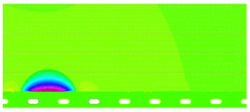
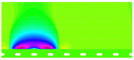
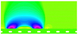
Figure 2.1: The first three horizontal filters $\psi_{1},\psi_{2}$ and $\psi_{3}$. The four horizontal lines correspond to $d$, $3d$, $5d$ and $7d$, where $d$ is the distance between the electrodes. Since the object to be imaged is located at distance $d$ (the first line), $\psi_{1},\psi_{2}$ and $\psi_{3}$ have been set to zero below that line. They are normalized so that $\max\psi_{k}=1$ for each $k$. Warmer colours represent higher values, followed by blue, then green around $0$ and yellow for negative values. The computation was made on a larger domain, with $14$ electrodes, with Freefem++[13], on a fine mesh, using $P2$ elements.

It is worth noting that, for algorithm testing purposes, it is possible to construct closed form qualitatively satisfactory approximation formulas for $\psi_{k}$. The advantage of such approximations is that they do not require the use of a finite element solver. We remind the reader that the Green function for a one dimensional periodic array of period $1$ in the direction $x_{1}$ is given by [3, 9]

$$G(x_{1},x_{2})=-\frac{1}{4\pi}\log\left(\sinh\left(\pi x_{2}\right)^{2}+\sinh\left(\pi x_{1}\right)^{2}\right)+\frac{1}{2}\left|x_{2}\right|.$$ (2.8)

It satisfies, in the sense of distributions

$$-\Delta G=\sum_{n\in\mathbb{Z}}\delta\left((x_{1},x_{2})-(n,0)\right).$$

Given a small parameter $\epsilon_{0}$, we can construct a function $f_{N}$ such that

$$\Delta f_{N}=0\text{ for }x_{2}\geq\epsilon_{0},\,f\left(0,\epsilon_{0}\right)=1\text{ and }f\left(n,\epsilon_{0}\right)=0\text{ for all }n=\left\{-N,\ldots,-1,1,\ldots,N\right\},$$

by finding the $N+1$ coefficients $\alpha_{0},\ldots,\alpha_{N}$ solving the linear system

$$M_{N}\left[\begin{array}[]{c}\alpha_{0}\\ \vdots\\ \vdots\\ \alpha_{N}\end{array}\right]=\left[\begin{array}[]{c}1\\ 0\\ \vdots\\ 0\end{array}\right],$$ (2.9)

where for all $1\leq i,j\leq N+1$,

$$M_{ij}=G(\frac{i-1}{j},\epsilon_{0}).$$

The function $f_{N}$ is then given by

$$f_{N}\left(x,y\right)=\sum_{k=0}^{N}\alpha_{k}G\left(\frac{x_{1}}{k+1},\frac{x_{2}}{k+1}\right).$$

An approximation for $\psi_{k}$ is then

$$\tilde{\psi}_{k}(x,y)=-\nabla f_{N}\left(x,y\right)\cdot\nabla f_{N}\left(x-k,y\right).$$

This approximates $u^{0}$, the background solution of the capacity problem (2.1), by a periodic solution in $x_{1}$ of large period $N$, which cancels periodically with period $1$ along the line $x_{2}=\epsilon_{0}$ when $x_{1}$ is an integer and not a multiple of $N$. Provided that $N$ is chosen large enough, $f_{N}$ is locally qualitatively similar to $u$. One example is represented in 2.2. Naturally, because $G$ given by 2.8 does not contain any information about the shape of the electrodes, they do not correspond precisely to 2.1, but they capture the main features of these weights. Regarding the solvability of system (2.9), notice that after one step of Gaussian elimination, the $N$-by-$N$ matrix $M^{(2)}$ has its entries given by the somewhat simpler formula

$$M_{ij}^{(2)}=\ln\left(1+\frac{\sinh\left(\pi\frac{i}{j+1}\right)^{2}}{\sinh\left(\pi\frac{\epsilon_{0}}{j+1}\right)^{2}}\right).$$

And this matrix turns out to be well conditioned numerically, even for large $N$.

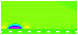
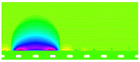
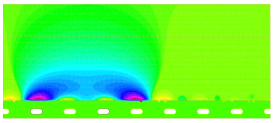
Figure 2.2: The first three horizontal approximate horizontal filters $\tilde{\psi}_{1},\tilde{\psi}_{2}$ and $\tilde{\psi}_{3}$. Computed with $N=16,$and $\epsilon_{0}=d/10.$

2.3 Interpreting the rotational data as a filtered Radon transform

To fix ideas, let us assume that the axis of rotation of the imaging device is the line of direction $(0,0,1)$, which passes through the origin. Suppose the solutions of (2.3), named $\left(u_{i}^{0}\right)_{1\leq i\leq N}$ correspond to $\theta=0$. After a rotation of an angle $\theta$, they become $u_{i}^{0,\theta}(x,y)=u_{i}^{0}\left(R_{-\theta}\underline{x}\right)=u_{i}^{0}\left(\left[\begin{array}[]{cc}\cos\theta&\sin\theta\\ -\sin\theta&\cos\theta\end{array}\right]\left[\begin{array}[]{c}x\\ y\end{array}\right],z\right)$. Thus the measured data becomes

$$\Delta C_{ij}^{\theta} \approx\int_{\mathbb{R}^{3}}\varepsilon_{0}\left(\varepsilon_{r}\left(\underline{x}\right)-1\right)\left(\nabla u_{j}^{0}\cdot\nabla u_{i}^{0}\right)\left(R_{-\theta}\underline{x}\right)\text{d}x\text{d}y\text{d}z,$$

$$=\int_{\mathbb{R}^{3}}\varepsilon_{0}\left(\varepsilon_{r}\left(R_{\theta}\underline{x}\right)-1\right)\left(\nabla u_{j}^{0}\cdot\nabla u_{i}^{0}\right)\left(\underline{x}\right)\text{d}x\text{d}y\text{d}z.$$ (2.10)

In particular, formula (2.7) becomes

$$H_{i,k}^{\theta}\approx\int_{\mathbb{R}^{3}}\varepsilon_{0}\left(\varepsilon_{r}\left(R_{\theta}\underline{x}\right)-1\right)\psi_{k}\left(\underline{x}-x_{i},z\right)\text{d}x\text{d}y\text{d}z,$$ (2.11)

with $x_{i}=\left(i-n-1\right)d\in\left\llbracket-nd,\left(n-k\right)d\right\rrbracket$ . But for the fact that the filter (or weight) $\psi_{k}$ is not constant on its support, $H_{i,k}^{\theta}$ represents the planar Radon Transform of the vertically averaged value of $\varepsilon_{0}\left(\varepsilon_{r}-1\right)$ on the support of $\psi_{k}$.

2.4 Incorporating practical sensor design constraints

The model we introduced is a simplification of the design used in practice. The transmitting and receiving electrodes are distinct sets, as represented in 2.3. The receiving electrode is grounded, whereas the non-receiving electrodes are floating, that is, the potential $u$ satisfies a Neumann (no flux) boundary condition on their surface.

Figure 2.3: Transmitting and receiving electrodes. The transmitting electrodes are represented in blue and connected to the hardware below. The receiving electrodes are connected to the hardware above.

Such a modification changes the shape of the flux, and therefore the definition of weight functions $\psi_{k},k=1,\ldots,4$, $\phi_{k},k=1,\ldots,4$ and $\zeta$; it does not otherwise affect the analysis in a significant manner otherwise. To be precise (2.7) still holds, but the two variable functions $\psi_{k}$ are now given by

$$\psi_{k}=\nabla u_{t}^{k}(x,z)\cdot\nabla u_{r}^{k}(x,z),$$

where for every $k$, both $u_{t}^{k}$ and $u_{r}^{k}$ satisfy different boundary conditions – in contrast to the previous situation where only one potential $u_{0}$ was needed. The potentials $u_{t}^{k}$ and $u_{r}^{k}$ satisfy the same equation and boundary condition away from the electrodes, which is

$$\begin{cases}\partial_{x}\left(\varepsilon_{0}\partial_{x}u_{t/r}^{k}\right)+\partial_{x}\left(\varepsilon_{0}\partial_{z}u_{t/r}^{k}\right)=0&\text{in }\text{$\mathbb{R}\times\left(0,\infty\right)\setminus\cup_{i=-\infty}^{\infty}I_{i}$}\\ \varepsilon_{0}\partial_{z}u_{t/r}^{k}\left(x_{1},0\right)=0,&\text{at }x_{2}=0\\ {\displaystyle\lim_{\left|\underline{x}\right|\to\infty}}u_{t/r}^{k}\left(\underline{x}\right)=0.\end{cases},$$

On the electrodes $u_{t}^{k}$ and $u_{r}^{k}$ satisfies the boundary conditions

$$\begin{cases}u_{t/r}^{k}=1&\text{on }\partial I_{0}\\ u_{t/r}^{k}=\alpha&\text{on }\partial I_{2m},\text{for every }m\in\mathbb{Z}\\ \varepsilon_{0}\partial_{\nu}u_{t/r}^{k}=0&\text{ on }\partial I_{2l+1},\text{for all }l\in\mathbb{Z}\text{ such that }l\neq k-1\\ u_{t/r}^{k}=\beta&\text{on }\partial I_{2k-1}.\end{cases},$$

with $(\alpha,\beta)=(1,0)$ for $u_{t}^{k}$ and $(\alpha,\beta)=(0,1)$ for $u_{r}^{k}$ respectively. In 2.4 we represent the functions $\psi_{1}$, $\psi_{2}$ and $\psi_{3}$, using the same colour scale as in 2.1 and 2.2. The horizontal symmetry is broken, as we should expect, since the boundary conditions of the Electrodes nearest the transmitter and the receiver are different. The weight $\psi_{1}$is the most significantly different from the others, as it takes both positive and negative values within its support. The overall support still roughly describes the arch intuited in the introduction, whereby higher strata are reached by more distant electrodes. After inversion, the data can thus be interpreted as several 2 dimensional horizontal cross sections of the permittivity, at different depths – a $2d+1$ imaging device.

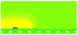
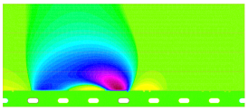
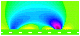
Figure 2.4: The first three horizontal approximate horizontal filters $\psi_{1},\psi_{2}$ and $\psi_{3}$, taking into account the Transmitter/Receiver distinction. Computed with FreeFem++ [13].

3 Experimental data

A Radon transform inversion was performed on the experimental data obtained from the rotating imaging device. Here, $n=27$ (55 electrodes), and $p=180$, which means measurements were recorded after a each $1^{0}$ rotation. The Matlab function iradon was applied to the resulting data, with linear interpolation and a Hamming filter.

In 3.1(1) we see the result of the lowest layer, the one closest to the sensor, corresponding to the data $H_{1}^{\theta}(1\ldots 2n)$. The shape of the hand is clearly visible. Levels of darkness indicate hints of lower and higher densities above. This can be expected: the field really reaches much more than simply the lowest level.

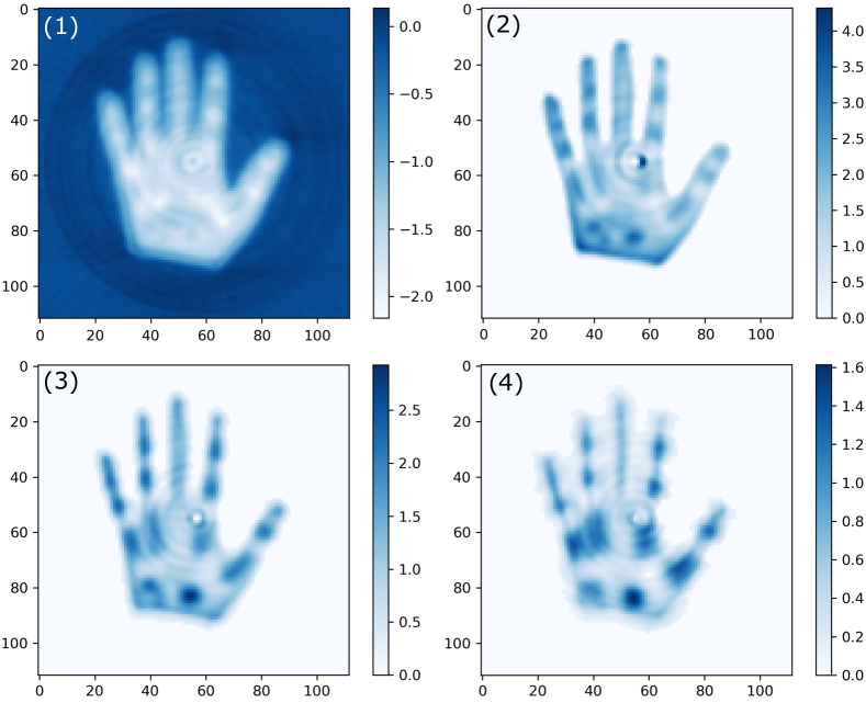
Figure 3.1: (1 - 4) Images reconstructed from $H_{1}$, $H_{2}$, $H_{3}$ and $H_{4}$ (Layers 1 - 4), corresponding to data from nearest, 2nd, 3rd and 4th nearest electrode pairs.

In 3.1(2) we show the second layer, namely, the inversion of $H_{2}^{\theta}(1\ldots 2n-1)$. A more defined hand appears, and the silver-inked trenches appear more marked than the empty trenches. We report the third neighbour data inversion in 3.1(3), and the fourth neighbour data in 3.1(4). As more features are lost with depth, the trenches become more defined. Additionally, the trenches with missing silver ink do not appear on the images due to the high contrast caused by the silver ink.

4 Conclusion, discussion, and future direction

We have described and modelled a coplanar non invasive non destructive capacitive imaging device. It is multiplexing, namely, individual electrodes can be measured independently. Together with a rotating platform, this allows to obtain Radon-like data, which, when inverted provides very good images of the model hand at different depth. It could seem remarkable that a Radon transform could be successfully used for ECT, as this is not a wave propagation problem. The link between EIT and generalized Radon Transform was established in [23] in the analysis of the Back Projection Algorithm [5] and further studied in [6, 17]. Our pictures are a naive double Radon inversion, namely, an actual radon inversion in the plane direction for electrodes of increasing distance, and then a ‘further away means deeper’ heuristic when reading the pictures. This calls for a proper justification, and a more quantitative algorithm, but the pictures obtained are encouraging. The images provided are truly raw data: no AI or compensation has been performed for the various weights involved. The cross data measurements have not been used in this application; they provide a convenient tool to localise horizontally the object at hand. Here, the location of the object was clearly visible. This data corresponds to measurements at one time point. We are investigating what is the best way to make use of various data time points, to enrich or improve the data collected. The quality of the images already obtained encourages us look for optimal reconstruction methods. The advantage of the one we have used here is that it used off-the-shelf algorithms, and data acquisition is very fast, as only a few milliseconds are required for each angle.

References

- [1] A. Adler, R. Gaburro, and W. Lionheart, Electrical Impedance Tomography, Springer New York, New York, NY, 2015, pp. 701–762.
- [2] K. J. Alme and S. Mylvaganam, Electrical capacitance tomography – sensor models, design, simulations, and experimental verification, IEEE Sensors Journal, 6 (2006), pp. 1256–1266.
- [3] H. Ammari and H. Kang, Polarization and moment tensors. With applications to inverse problems and effective medium theory., New York, NY: Springer, 2007.
- [4] R. Banasiak and M. Soleimani, Shape based reconstruction of experimental data in 3d electrical capacitance tomography, NDT and E International, 43 (2010), pp. 241–249. cited By 36.
- [5] D. C. Barber and B. H. Brown, Applied Potential Tomography, Journal of Physics E-Scientific Instruments, 17 (1984), pp. 723–733.
- [6] C. A. Berenstein and E. Casadio Tarabusi, Inversion formulas for the -dimensional Radon transform in real hyperbolic spaces, Duke Math. J., 62 (1991), pp. 613–631.
- [7] L. Borcea, Electrical impedance tomography, Inverse Problems, 18 (2002), p. R99.
- [8] L. Borcea, V. Druskin, and F. G. Vasquez, Electrical impedance tomography with resistor networks, Inverse Problems, 24 (2008), p. 035013.
- [9] R. E. Collin, Field theory of guided waves. 2nd ed., Oxford: Oxford Univ. Press; New York, NY: IEEE, 2nd ed. ed., 1991.
- [10] R. Dautray and J.-L. Lions, Mathematical analysis and numerical methods for science and technology. Volume 1: Physical origins and classical methods. With the collaboration of Philippe Bénilan, Michel Cessenat, André Gervat, Alain Kavenoky, Hélène Lanchon. Transl. from the French by Ian N. Sneddon. 2nd printing., Berlin: Springer, 2nd printing ed., 2000.
- [11] C. Dias and R. Igreja, A method of recursive images to obtain the potential, the electric field and capacitance in multi-layer interdigitated electrode (ide) sensors, Sensors and Actuators A: Physical, 256 (2017), pp. 95 – 106.
- [12] S. Gupta and K. J. Loh, Noncontact electrical permittivity mapping and ph-sensitive films for osseointegrated prosthesis and infection monitoring, IEEE Transactions on Medical Imaging, 36 (2017), pp. 2193–2203.
- [13] F. Hecht, New development in freefem++., J. Numer. Math., 20 (2012), pp. 251–265.
- [14] D. Holder, Electrical impedance tomography : methods, history, and applications, Institute of Physics Pub, Bristol Philadelphia, 2005.
- [15] X. Hu and W. Yang, Planar capacitive sensors – designs and applications, Sensor Review, 30 (2010), pp. 24–39.
- [16] R. Igreja and C. Dias, Extension to the analytical model of the interdigital electrodes capacitance for a multi-layered structure, Sensors and Actuators A: Physical, 172 (2011), pp. 392 – 399.
- [17] H. Isozaki, Inverse boundary value problems in the horosphere—a link between hyperbolic geometry and electrical impedance tomography, Inverse Probl. Imaging, 1 (2007), pp. 107–134.
- [18] H. M. Mamigonians, Method and sensor for sensing the electrical permittivity of an object, March 2015.
- [19] A. V. Mamishev, K. Sundara-Rajan, F. Yang, Y. Du, and M. Zahn, Interdigital sensors and transducers, Proceedings of the IEEE, 92 (2004), pp. 808–845.
- [20] H. J. Pandya, K. Park, and J. P. Desai, Design and fabrication of a flexible mems-based electro-mechanical sensor array for breast cancer diagnosis, Journal of Micromechanics and Microengineering, 25 (2015), p. 075025.
- [21] V. Rimpiläinen, L. M. Heikkinen, and M. Vauhkonen, Moisture distribution and hydrodynamics of wet granules during fluidized-bed drying characterized with volumetric electrical capacitance tomography, Chemical Engineering Science, 75 (2012), pp. 220 – 234.
- [22] A. Samorè, M. Guermandi, S. Placati, and R. Guerrieri, Parametric detection and classification of compact conductivity contrasts with electrical impedance tomography, IEEE Transactions on Instrumentation and Measurement, 66 (2017), pp. 2666–2679.
- [23] F. Santosa and M. Vogelius, A backprojection algorithm for electrical impedance imaging, SIAM J. Appl. Math., 50 (1990), pp. 216–243.
- [24] M. Soleimani and W. Lionheart, Nonlinear image reconstruction for electrical capacitance tomography using experimental data, Measurement Science and Technology, 16 (2005), pp. 1987–1996. cited By 164.
- [25] C. Tholin-Chittenden and M. Soleimani, Planar array capacitive imaging sensor design optimization, IEEE Sensors Journal, 17 (2017), pp. 8059–8071.
- [26] C. Tholin-Chittenden and M. Soleimani, Planar array capacitive imaging sensor design optimization, IEEE Sensors Journal, 17 (2017), pp. 8059–8071. cited By 0.
- [27] G. Uhlmann, Electrical impedance tomography and calderón’s problem, Inverse Problems, 25 (2009), p. 123011.
- [28] J. Webster, Electrical impedance tomography, Adam Hilger, Bristol New York, 1990.
- [29] Z. Ye, R. Banasiak, and M. Soleimani, Planar array 3d electrical capacitance tomography, Insight - Non-Destructive Testing and Condition Monitoring, 55 (2013), pp. 675–680.