Thermal fluctuations in antiferromagnetic nanostructures

Abstract

A theoretical model is developed that can accurately analyze the effects of thermal fluctuations in antiferromagnetic (AFM) nano-particles. The approach is based on Fourier series representation of the random effective field with cut-off frequencies of physical origin at low and high limits while satisfying the fluctuation-dissipation theorem at the same time. When coupled with the formalism of a Langevin dynamical equation, it can describe the stochastic Néel vector dynamics with the AFM parameters, circumventing the arbitrariness of the commonly used treatments in the micro-magnetic simulations. Subsequent application of the model to spontaneous Néel vector switching provides a thermal stability analysis of the AFM states. The numerical simulation shows that the AFM states are much less prone to the thermally induced accidental flips than the ferromagnetic counterparts, suggesting a longer retention time for the former.

I Introduction

Thermal fluctuations are evidently considered a destructive factor as the electronic devices shrink to the nanoscale dimensions. However, the situation is not so clear cut in spintronic devices based on magnetic switching in nano-particles. While spontaneous reversal of the magnetization negatively affects the lifetime of the binary states in a magnetic memory or logic, thermal magnetic fluctuations can be exploited to accelerate or even determine the magnetization flip in ferromagnetic (FM) devices for heat-assisted magnetic recording. Berkov2004 ; Atxitia2009 ; Galatsis2009 ; Vogler2016 Furthermore, other widely adopted mechanisms such as spin transfer torque require a slight misalignment for the desired magnetization rotation. Slavin2009

The theoretical approaches to the modeling of thermal effects are based on stochastic itinerancy in the magnetization orientation induced by a fluctuating effective field $\mathbf{H}_{th}(t)$ that essentially supposes a white noise satisfying Brown1963

$$\left\langle H_{th,j}(t)H_{th,j^{\prime}}(t^{\prime})\right\rangle=D_{\mathrm{FM}}\delta_{j,j^{\prime}}\delta(t-t^{\prime}).$$ (1)

The amplitude of un-correlated random component $j=x,y,z$ of the vector $\mathbf{H}_{th}(t)$ is regulated by the fluctuation-dissipation theorem

$$D_{\mathrm{FM}}=\frac{2\alpha_{\mathrm{G}}k_{B}T}{\gamma M_{\mathrm{FM}}V},$$ (2)

where $\alpha_{\mathrm{G}}$, $\gamma$, $M_{\mathrm{FM}}$, and $V$ denote the Gilbert damping parameter, gyromagnetic ratio, magnetization, and volume of the FM mono-domain, respectively. Incorporating $\mathbf{H}_{th}(t)$ into the stochastic Landau-Lifshitz-Gilbert equation (LLG) in the form of a white noise, while satisfying the requirement of no correlation at different times as described [Eq. (1)], gives rise to the mathematical problem of accounting for a ”rapidly varying, highly irregular function”. Gardiner Further, this treatment of $\mathbf{H}_{th}(t)$ leads to an infinite variance.

In the quantitative studies, micro-magnetic simulations have been used widely that treat the FM particle as an ensemble of magnetic cells with a FM exchange interaction between them. Magnetism2007 Each cell is subjected to a random field $\mathbf{H}_{th}(t)$ which is not correlated with those of the neighbors. Likewise, the random fields in the time-domain implementation are assumed invariable once selected during each time interval $\Delta t$ (in the range of 20$-$100 ps) and without interdependence between the time steps. This approach recovers a finite variance Magnetism2007

$$\left\langle H_{th,j}^{2}(t)\right\rangle=\frac{2\alpha_{\mathrm{G}}k_{B}T}{\gamma M_{\mathrm{FM}}V\Delta t}$$ (3)

that is also in compliance with the fluctuation-dissipation theorem discussed above. The arrangement adopted in the time domain is in recognition of the finite auto-correlation time $\tau_{c}$ in the magnetization dynamics of the realistic systems in contrast to the no correlation assumption of Eq. (1). Magnetism2007 Nonetheless, the arbitrariness in the time discretization $\Delta t$ of the stochastic fields adds a significant uncertainty in the final results. Roma2014 Similarly, concerns exist on applicability of the bulk parameters $\alpha_{\mathrm{G}}$, $M_{\mathrm{FM}}$ and $V$ to (sub-)nanometer scale cells with arbitrarily chosen sizes and shapes.

The difficulties of the conventional treatment are compounded in the simulation of more complex antiferromagnetic (AFM) dynamics. The AFMs have recently received much attention due to their potential advantages in spintronic applications over the FM counterparts. Jungwirth2016 Accordingly, accurate description of Néel vector dynamics is crucial in the realistic conditions at the ambient temperature. In this work, we develop an alternative approach for the effect of the random thermal fluctuations in the AFM structures based on a Langevin-type dynamical equation. The model is then adopted to analyze thermal stability of the AFM states in the nano-scale dimensions (i.e., lifetimes) highlighting its potential applications.

II Thermal field modeling in AFMs

Treating the ratcheted field effect on AFM stochastic dynamics as antiparallelly ordered FM cells in the manner of micro-magnetic simulations poses challenges beyond those faced by FM counterparts. For one, the dynamic equations for AFM (or Néel) vector $\mathbf{L}$ ($=\mathbf{M}_{1}-\mathbf{M}_{2}$, where $\mathbf{M}_{1}$ and $\mathbf{M}_{2}$ are sublattice magnetizations) involve the time derivative $\frac{d}{dt}\mathbf{H}_{th}(t)$ that is not compatible with abrupt changes in $\mathbf{H}_{th}(t)$ often associated with the thermal fields. Even when this singularity is somehow avoided, such a step-function treatment would evidently overestimate the high frequency components of the noise, resulting in parasitic excitation of spurious optical magnons in the AFM. Another difficulty stems from the fact that the correlation time of thermal fields may be comparable to the temporal scale of AFM dynamics which is much faster than the FM counterparts. Atxitia2009 In fact, the effect of a finite correlation time was a subject of a detailed investigation even for much slower FM dynamics in the case of colored thermal noise. Tranchida2016 In general, an increase in the auto-correlation time would enhance the inertial effects and lead to stronger magnetization damping. Thus, the desired solution is a representation of the thermal fields with a finite, physically determined correlation time that can be incorporated into the stochastic Néel vector dynamics for numerical evaluation. An alternative theory based on the Fokker-Planck equation was proposed previously to describe small deviations around the deterministic trajectory of the Néel vector. Gomonay2013 In contrast, the approach pursued here can lead to an exact solution of the stochastic equation that is applicable to large fluctuations as well.

The thermal noise model under consideration is based on a spectral representation of $\mathbf{H}_{th}(t)$ in contrast to the introduction of random step functions in the time domain as it allows a number of advantages. First, the response of a damped AFM vector indicates that the random fluctuations via $\mathbf{H}_{th}(t)$ also decay within the corresponding characteristic time $\tau_{m}$ (i.e., the longest time of relevance). Thus, $2\pi/\tau_{m}$ essentially provides the truncation frequency in the noise spectrum. Similarly, the auto-correlation time $\tau_{c}$ (or more precisely, its inverse) can be incorporated as the upper bound in the high frequencies. Further, the association of $\tau_{m}^{-1}$ to the broadening $\delta_{r}$ of AFM resonant frequency ($\delta_{r}=2\pi/\tau_{m}$) offers a physical ground for the discretization of the spectral domain in the comparable intervals $\Delta\omega$ ($\approx\delta_{r}$). This frequency uncertainty in each interval conveniently enables us to approximate the desired spectral function with an average over $\Delta\omega$ around a typical frequency, followed by a summation over the allowed frequency domain. In other words, the AFM response on the actual thermal noise in a dissipative medium is virtually equivalent to a series of harmonic oscillations (i.e., Fourier expansion) with random amplitudes and frequencies $n\Delta\omega$ ($n=1,2,...,N$, where $N=2\pi/\tau_{c}\Delta\omega\approx\tau_{m}/\tau_{c}$). As such, a similar Fourier series treatment can also be used for $H_{th,j}(t)$.

The underlying rationale of the discrete treatment described above can be seen more clearly by considering the formal conversion of the response to the white noise. Since the magnetic permeability $\chi(\omega)$ (treated here like a scalar for convenience in the notation) drives the dynamical response $m(\omega)$, the resulting stochastic motion is expressed as ($j=x,y,z$):

$$m_{j}(t)=\int\chi(\omega)H_{th,j}(\omega)e^{i\omega t}d\omega=\sum_{n}\int_{0}^{\Delta\omega}\chi(n\Delta\omega+\omega)H_{th,j}(n\Delta\omega+\omega)e^{i(n\Delta\omega+\omega)t}d\omega.$$ (4)

If $\Delta\omega$ is small enough to keep $\chi(n\Delta\omega+\omega)$ almost constant as $\omega$ varies in the interval $(0,\Delta\omega)$, Eq. (4) can be reduced to a discrete sum $\sum_{n}\chi(n\Delta\omega)e^{in\Delta\omega t}H_{jn}$, where $H_{jn}=\int_{0}^{\Delta\omega}H_{th,j}(n\Delta\omega+\omega)e^{i\omega t}d\omega$. Following the same theoretical underpinning, it can also be shown explicitly that $H_{jn}$ corresponds to the $n$th Fourier component of $H_{th,j}(t)$ in the complex space: i.e.,

$$H_{th,j}(t)=\int H_{th,j}(\omega)e^{i\omega t}d\omega=\sum_{n}e^{in\Delta\omega t}\int_{0}^{\Delta\omega}H_{th,j}(n\Delta\omega+\omega)e^{i\omega t}d\omega=\sum_{n}H_{jn}e^{in\Delta\omega t}.$$ (5)

As the field $H_{th,j}$ is random, so is $H_{jn}$. With explicit imposition of the upper and lower bounds in the noise spectrum discussed earlier, the thermal field can finally be written as a series of harmonic perturbations with random amplitudes $a_{jn}$ and $b_{jn}$ in the following form:

$$H_{th,j}(t)=\sum_{n=1}^{N}a_{jn}\sin(n\Delta\omega t)+\sum_{n=1}^{N}b_{jn}\cos(n\Delta\omega t).$$ (6)

Note that this noise expression applies only for a duration up to $2\pi/\Delta\omega$ in the time domain due to the relaxation (i.e., $\sim\tau_{m}$). A time period longer than this interval requires refreshing the selection of amplitude for each component. Thus, $H_{th,j}(t)$ (as well as the associated quantities such as the correlation function) is not periodic in time. Nonetheless, it is continuous in $t$ ensured by a condition imposed on $a_{jn}$ and $b_{jn}$, which stems from the stationarity of the random process (see the discussion below).

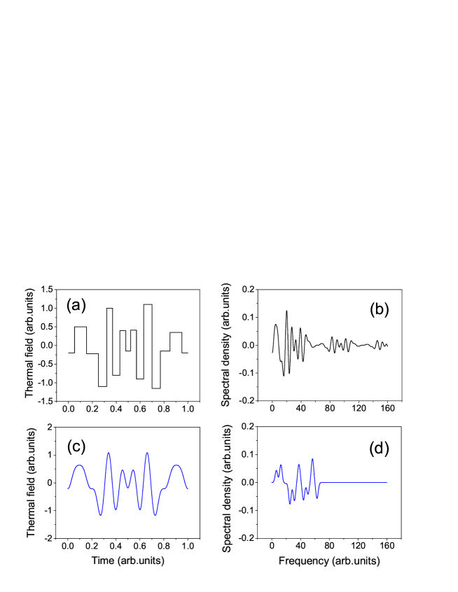
Figure 1: Example of white noise simulation in the time domain in terms of (a) random steps and (c) harmonic oscillations with random amplitudes. While the corresponding spectral density of the step functions is unrestricted in the frequency domain [(b)], the harmonics can be confined in a physically valid range [(d)]. The frequency of each harmonic is assumed to diffuse due to a finite relaxation time.

The approach based on Eq. (6) avoids unphysical features attributed to the white noise treatment of Eq. (1) including the virtually constant spectral density at arbitrary small frequencies and the excitation of very high frequency perturbations (see Fig. 1). It also circumvents the singularities associated with the derivatives of the step-function representation of the random thermal field. Tsiantos2003 As discussed above, the frequency interval $\Delta\omega$ can be associated with the broadening $\delta_{r}$ of AFM resonance frequency (e.g., $\Delta\omega\approx\delta_{r}=2\pi/\tau_{m}$), for which experimental measurements are generally available in the literature. Similarly, the estimation of the upper bound (i.e., $\tau_{c}^{-1}$) can be reliably achieved in term of the microscopic theory. An alternative is to treat $\tau_{c}$ as a phenomenological parameter following the earlier studies for the corresponding problem in the FM particles. Magnetism2007 Needless to say, both of them (i.e., $\tau_{m}$ and $\tau_{c}$) are also a function of temperature as with other relevant parameters of the AFM (including damping constant, resonance frequency, etc.). This dependence can be accounted for by simply adjusting the numerical values according to the the ambient conditions of interest.

On the other hand, the thermal field must satisfy a restriction on the correlation function imposed by the stationarity of the fluctuations as well; i.e.,

$$g_{j,j^{\prime}}(t^{\prime},t)=\delta_{j,j^{\prime}}\left\langle H_{th,j}(t^{\prime})H_{th,j}(t)\right\rangle,$$ (7)

where $\left\langle...\right\rangle$ is an average over the ensemble of identical magnetic particles. The function $g_{j,j^{\prime}}(t^{\prime},t)$ that depends on $t^{\prime}-t$ can be calculated in terms of Eq. (6) so long as the random parameters are statistically independent, i.e., $\left\langle b_{jn}a_{j^{\prime}n^{\prime}}\right\rangle=0$, $\left\langle b_{jn}b_{j^{\prime}n^{\prime}}\right\rangle=\delta_{j,j^{\prime}}\delta_{n,n^{\prime}}\left\langle b_{n}^{2}\right\rangle$, $\left\langle a_{jn}a_{j^{\prime}n^{\prime}}\right\rangle=\delta_{j,j^{\prime}}\delta_{n,n^{\prime}}\left\langle a_{n}^{2}\right\rangle$ and the premise $\left\langle b_{jn}\right\rangle=\left\langle a_{jn}\right\rangle=0$. Stationarity of the random process $H_{th}(t)$ also imposes equality $\left\langle b_{n}^{2}\right\rangle=\left\langle a_{n}^{2}\right\rangle$ such that Eq. (7) reduces to

$$g(t^{\prime},t)=\frac{1}{2}\sum_{n=1}^{N}\left(\left\langle a_{n}^{2}\right\rangle+\left\langle b_{n}^{2}\right\rangle\right)\cos[\Delta\omega n(t^{\prime}-t)]=g(t^{\prime}-t).$$ (8)

Here, subscript $j$ is omitted for simplicity. In the limit of white noise (i.e., $\Delta\omega\rightarrow 0$ and $N\rightarrow\infty$), this equation obviously reproduces the $\delta$-correlation as supposed in Eq. (1), provided that $\left\langle b_{n}^{2}\right\rangle=\left\langle a_{n}^{2}\right\rangle$ is a constant. Thus, the value $\frac{1}{2}\left(\left\langle a_{n}^{2}\right\rangle+\left\langle b_{n}^{2}\right\rangle\right)$ determines the spectral density of the correlation function in Eq. (8):

$$(H_{th}^{2})_{\omega}=\frac{1}{2\delta_{r}}\sum_{n=1}^{N}(\left\langle a_{n}^{2}\right\rangle+\left\langle b_{n}^{2}\right\rangle).$$ (9)

The set of parameters $\left\langle b_{n}^{2}\right\rangle$ relates to magnetic susceptibility $\chi(\omega)=\chi^{\prime}(\omega)+i\chi^{\prime\prime}(\omega)$ via the fluctuation-dissipation theorem. In the limit of high temperature, this theorem prescribes

$$(H_{th}^{2})_{\omega}=2\frac{k_{B}T}{\hbar\omega}\frac{\hbar\chi^{\prime\prime}(\omega)}{\left|\chi(\omega)\right|^{2}}.$$ (10)

We apply the AFM permeability at zero external field in the form Andreev1980

$$\chi(\omega)=-\frac{2}{D(\omega)}V\gamma M_{L}(\gamma H_{an}+i\alpha_{\mathrm{A}}\omega);$$ (11)

$$D(\omega)\simeq\omega^{2}-2\gamma^{2}H_{ex}H_{an}-2i\alpha_{\mathrm{A}}\omega\gamma(H_{ex}+H_{an}),$$ (12)

where $M_{L}$ denotes the saturation magnetization ($=\left|\mathbf{L}\right|$ in equilibrium), $H_{ex}$ and $H_{an}$ ($\ll H_{ex}$) stand for the interlayer exchange field and the anisotropy field, respectively, and $\alpha_{\mathrm{A}}$ is a damping constant which is associated with each AFM sublatice (also related to the resonance width $\delta_{r}=\alpha_{\mathrm{A}}\gamma H_{ex}$). The validity around the zero-field resonance frequency $\omega_{r}=\sqrt{2\gamma^{2}H_{ex}H_{an}}$ is assumed for the permeability expression given above.

A straightforward calculation with a sufficiently small $\alpha_{\mathrm{A}}$ provides the power of the thermal field as

$$(H_{th}^{2})_{\omega}=\frac{2\eta k_{B}T}{\gamma M_{L}V}.$$ (13)

This expression formally resembles the thermal effect in a FM mono-domain [see Eq. (2)] so long as the modified AFM damping parameter $\eta$ ($=\alpha_{\mathrm{A}}\sqrt{H_{ex}/H_{an}}$) corresponds to the FM Gilbert damping constant $\alpha_{\mathrm{G}}$. Comparison of Eqs. (13) and (9) yields

$$\frac{1}{2}(\left\langle b_{n}^{2}\right\rangle+\left\langle a_{n}^{2}\right\rangle)=\delta_{r}\frac{2\eta k_{B}T}{\gamma M_{L}V}.$$ (14)

It is convenient to generate the Fourier amplitudes $a_{n}$, $b_{n}$ of the thermal field in terms of the random numbers $\alpha_{n}$, $\beta_{n}$ of the Gaussian distribution with variance of $1$; i.e.,

$$\frac{1}{2N}\sum_{n=1}^{N}\left\langle\beta_{n}^{2}+\alpha_{n}^{2}\right\rangle=1.$$ (15)

Consequently, Eq. (14) imposes relations $a_{n}=\overline{B}\alpha_{n}$ and $b_{n}=\overline{B}\beta_{n}$ with the scaling

$$\overline{B}=\frac{\delta_{r}}{\gamma}\left(\frac{2k_{B}T}{NKV}\right)^{1/2}$$ (16)

yielding the thermal field in dimensionless units as

$$\frac{\gamma H_{th}(t)}{\omega_{r}}=\frac{\delta_{r}}{\omega_{r}}\left(\frac{2k_{B}T}{NKV}\right)^{1/2}\left(\sum_{n=1}^{N}\alpha_{n}\sin n\delta_{r}t+\sum_{n=1}^{N}\beta_{n}\cos n\delta_{r}t\right),$$ (17)

where $K=M_{L}H_{an}$ is an anisotropy constant. This expression clearly gives the derivatives $dH_{th}(t)/dt$ in the form of smooth functions that can be directly included in the AFM dynamic equation.

III Langevin equation

The thermal field effect on the Néel vector dynamics can now be modeled in terms of the Lagrangian derived from the symmetry consideration. Andreev1980 ; Ivanov1995 The alternative approach based on the LLG equations for the coupled sublattice magnetizations $\mathbf{M}_{1}$ and $\mathbf{M}_{2}$ in an external field $\mathbf{H}$ (including the contribution $\mathbf{H}_{th}$ of thermal origin) as well as the internal exchange and anisotropy fields ($\mathbf{H}_{ex}$, $\mathbf{H}_{an}$) generates the same result when the AFM exchange coupling dominates over the others. The latter condition supposes the magnitude of the Néel vector $\left|\mathbf{L}\right|$ to remain unaltered under its rotation such that the unit vector $\mathbf{n=L/}\left|\mathbf{L}\right|$ is sufficient to uniquely determine the AFM state. Since the following analysis is limited to the AFMs of nano-scale sizes, the spatial variation of $\mathbf{L}$ can be safely omitted in the Lagrangian, which takes the form

$$\textswab{L}=\frac{M_{L}^{2}}{2\omega_{ex}^{2}}{\dot{\mathbf{n}}}^{2}-\frac{M_{L}^{2}}{\omega_{ex}^{2}}[{\dot{\mathbf{n}}}\times\mathbf{n]\cdot}\gamma\mathbf{H}+\frac{M_{L}^{2}}{2\omega_{ex}^{2}}[\mathbf{n\times}\gamma\mathbf{H}]^{2}-W(\mathbf{n}),$$ (18)

where ${\dot{\mathbf{n}}\equiv}\frac{d}{dt}\mathbf{n}$ and $\omega_{ex}^{2}=\gamma^{2}H_{ex}{M_{L}}$. We consider the typical case of a biaxial AFM with the density of anisotropy energy

$$W(\mathbf{n})=\frac{1}{2}(K_{x}n_{x}^{2}+K_{z}n_{z}^{2}),$$ (19)

where the constants $K_{x}$ ($<0$) and $K_{z}$ ($>0$) determine the easy $x$- and the hard $z$-axis, respectively. In addition, the magnetic anisotropy can be engineered via the shape and the strain of the AFM sample. Gomonay2014 The cubic and higher-order terms are neglected in Eq. (19). Accordingly, the anisotropy field $H_{an}$ now corresponds to $\left|K_{x}\right|/M_{L}$ [i.e., $\left|K_{x}\right|\leftrightarrow K$ in Eq. (17)].

Then, the magnetic relaxation toward the local minimum of $W(\mathbf{n},t)$ can be incorporated into the kinetic equation by way of a dissipation function

$$\textfrak{R}=\frac{\delta_{r}{M_{L}}^{2}}{\omega_{ex}^{2}}{\dot{\mathbf{n}}}^{2},$$ (20)

which can be given in terms of the homogeneous line width $\delta_{r}$ of the AFM resonance mentioned earlier. Note that this expression accounts for only the relativistic Gilbert-like relaxation. The effect of the exchange relaxation on $\mathbf{n}$ is expected to be relatively unimportant as it primarily affects the net magnetization of the AFM (i.e., $\mathbf{M}_{1}+\mathbf{M}_{2}$) rather than the actual dynamics of the Néel vector ($=\mathbf{M}_{1}-\mathbf{M}_{2}$) [see Ref. Gomonay2014, for a related discussion].

The corresponding Lagrange equation augmented with Eq. (20) describes the evolution of the AFM vector in the form of a Langevin second-order differential equation. Since the variation $\delta\mathbf{n}$ of unit vector $\mathbf{n}$ comes from its rotation around a vector $\delta\mathbf{\phi}$ by an infinitesimal angle $\left|\delta\mathbf{\phi}\right|$, the resulting expression takes the form

$$\mathbf{n}\times\left[{\ddot{\mathbf{n}}}-2({\dot{\mathbf{n}}}\times\mathbf{h})-(\mathbf{n}\times{\dot{\mathbf{h}}})+\mathbf{h}(\mathbf{n\cdot h})+\frac{\partial}{\partial\mathbf{n}}w(\mathbf{n})+2\frac{\delta_{r}}{\omega_{r}}{\dot{\mathbf{n}}}\right]=0$$ (21)

in dimensionless time $\omega_{r}t\rightarrow t$. Similarly, a normalized form is used for the field $\mathbf{H}$ (i.e., $\mathbf{h}=\gamma\mathbf{\mathbf{H/}}\omega_{r}$). Hereinafter, $\mathbf{h}$ corresponds to the normalized thermal field $\mathbf{h}_{th}$ assuming no contribution of other origins.

The actual independent variables are polar $\varphi$ and azimuthal $\theta$ angles of the unit vector $\mathbf{n}=(\sin\theta\cos\varphi,\sin\theta\sin\varphi,\cos\theta)$. Accordingly, Eq. (21) establishes the set of two second order differential equations

$$\ddot{\theta}=\frac{1}{2}\left[\dot{\varphi}^{2}+\kappa_{z}-\kappa_{x}\cos^{2}\varphi\right]\sin 2\theta-2\lambda\dot{\theta}$$ (22)

$$+2\dot{\varphi}\sin\theta(\mathbf{n}\cdot\mathbf{h})+(\dot{{h}_{x}}\sin\varphi-\dot{{h}_{y}}\cos\varphi)+F_{\theta}(\mathbf{h})$$

and

$$\ddot{\varphi}\sin^{2}\theta=\frac{\kappa_{x}}{2}\sin 2\varphi\sin^{2}\theta-\dot{\theta}\dot{\varphi}\sin 2\theta-2\lambda\dot{\varphi}\sin^{2}\theta$$ (23)

$$-2\dot{\theta}\sin\theta(\mathbf{n}\cdot\mathbf{h})+\cos\theta(\mathbf{n}\cdot\dot{\mathbf{h}})-\dot{{h}_{z}}+F_{\varphi}(\mathbf{h}),$$

where $\kappa_{z}=K_{z}/\left|K_{x}\right|$, $\kappa_{x}=K_{x}/\left|K_{x}\right|$, and $\lambda=\delta_{r}/\omega_{r}$. The quadratic-in-$\mathbf{h}$ terms $F_{\theta}(\mathbf{h})$ and $F_{\varphi}(\mathbf{h})$ have often been neglected for relatively small thermal fluctuations around the deterministic Néel vector traces. Gomonay2013 In contrast, these two terms cannot be ignored when the problem concerns spontaneous Néel vector switching through the barrier of anisotropy energy. The detailed expressions necessary in the latter case are given as

$$F_{\theta}(\mathbf{h})=\frac{1}{2}\sin 2\theta\left(-h_{x}^{2}\cos^{2}\varphi-h_{y}^{2}\sin^{2}\varphi+h_{z}^{2}\right)$$ (24)

and

$$F_{\varphi}(\mathbf{h})=\frac{1}{2}\sin^{2}\theta\sin 2\varphi(-h_{x}^{2}+h_{y}^{2}).$$ (25)

Since $\left\langle h_{x}^{2}\right\rangle=\left\langle h_{y}^{2}\right\rangle=\left\langle h_{z}^{2}\right\rangle$, the thermal field does not deviate the equilibrium position away from the stationary states $\mathbf{n}\|\pm\hat{\mathbf{x}}$ on average (which still permits flipping between them). The cross terms $h_{i}h_{j}$ ($i\neq j$) are dropped safely considering the uncorrelated nature of the fluctuations $h_{i}$ and $h_{j}$. Note that the stochastic equations given above [e.g., Eqs. (22) and (23)] can be readily applied to describe the Néel vector dynamics in the presence of the driving field as well as the thermal fluctuations. In such a case, the field $\mathbf{h}$ (thus, $\mathbf{H}$) needs to be expanded to include both contributions. An explicit Runge-Kutt method can be used for the time integration of the differential equations. The discretization step size for this numerical method depends on the correlation time, for which a fraction of $\tau_{c}$ is a convenient choice.

Compared to the evolution of FM nano-particle magnetization, the AFM Néel vector dynamics is much more complex due to several reasons. For instance, the relatively strong fluctuations may disturb the trajectory in such a manner that does not nudge the Néel vector out of the initial stable state. This phenomenon is related to the chiral dynamics of sublattice magnetizations. Similarly, the inertial behavior can play a considerable role unlike in the FM counterparts. Semenov2017 With strong damping (i.e., a lesser impact by inertia), one can expect that the Néel vector would be drawn closer to the saddle point of the anisotropy potential separating two energetically favorable regions. Under slow relaxation, on the other hand, the nearly free movement with inertia may migrate away from the saddle point, ultimately requiring a stronger excitation to overcome the barrier. At the same time, the rate of field variation (i.e., the slope $\frac{d}{dt}h$) affects the outcome along with its amplitude [see, for example, Eqs. (22) and (23)].

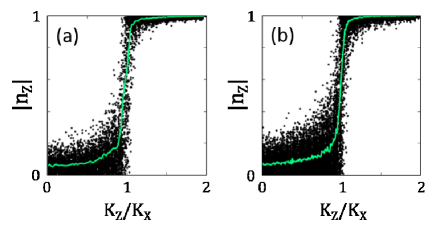
Figure 2: Thermal distribution of Néel vector equilibrium states (a) calculated in terms of the stochastic equations and (b) via random selections according to the Boltzmann probability function. The solid lines indicate the mean values of $n_{z}$. Parameters of AFM nano-particle are as discussed in the main text (see Sec. IV). While the easy $x$-axis anisotropy ($K_{x}$) is set at $-4.4\times 10^{5}$ erg/cm³, the $z$ direction varies from $K_{z}=0$ to $K_{z}=-8.8\times 10^{5}$ erg/cm³ making it the primary easy axis.

Nevertheless, the outcome of the stochastic treatment is expected to mimic the Boltzmann-type thermal distribution in equilibrium. As a test, a comparison is made in Fig. 2 between the two for a range of $z$-directional anisotropy values in a biaxial AFM at room temperature. The result physically corresponds to reorientation of the Néel vector along the $z$ direction ($|n_{z}|\rightarrow 1$) as the primary easy axis of the material switches from $x$ to $z$ (i.e., $K_{z}/K_{x}=0\rightarrow 2$). While Fig. 2(a) plots $100$ independent solutions of stochastic equations at each $K_{z}/K_{x}$ value (after a long but fixed duration $t$), the data points in Fig. 2(b) represent the same number of random selections for $\mathbf{n}$ from the Boltzmann distribution accounting for only the anisotropy energy; i.e., $\exp[-\frac{1}{2}(K_{x}n_{x}^{2}+K_{z}n_{z}^{2})/k_{B}T]$. The similarity between them is rather uncanny despite the drastic difference in the theoretical approaches. The observed small disparity in the variance may be attributed to the neglect of the ”kinetic” energy in the simple Boltzmann expression used in Fig. 2(b) [see the first term on the right-hand side in Eq. (18)]. The non-zero contribution of this (thermal) kinetic energy term tends to reduce the deviation away from the mean value (i.e., a tighter distribution).

IV Retention time evaluation

As an illustration of the ability to describe beyond the small fluctuations around the deterministic trajectory (e.g., Fig. 2), the dynamical model discussed above is adopted to study the problem of spontaneous Néel vector switching in AFM nanostructures. Evidently, the stability of a magnetic state against the thermal excitation is an issue of major significance in numerous applications of magnetic devices such as nonvolatile logic and memory. However, a corresponding analysis of the functional dependence in a parametrically closed form is difficult to achieve as in the theory of bistable dynamics that is quite sophisticated even for one-dimensional (1D) classical particles Melnikov91 or FM mono-domains. Kalmykov2004 Thus, the results of the Langevin dynamics may be more conveniently interpreted from an empirical standpoint of a particle escaping from a local minimum through thermal fluctuations in an open system. Smelyanskiy1997 A key feature commonly adopted in this context is the activation law for escape, or inversely, the retention time $t_{r}\sim\exp(\Delta_{b}/k_{B}T)$. Parameter $\Delta_{b}$ represents the effective activation energy that depends on the particular energetic profile, the spectral density of noise, and the correlation time as it was shown for a 1D classical system with a double-well potential. Dykman1990

To evaluate the escape rate, the numerical solutions are obtained in a sequence of $N_{i}$ iterations, each with the time interval $\tau_{m}$. As discussed above in Sec. II, random selection of the Fourier amplitudes is refreshed for each iteration by following the thermal noise model, while the initial state is set by the solution of the preceding time interval. This sequence is repeated until the number ($N_{sw}$) of observed switching events between the $n_{x}\approx\pm 1$ states reach a sufficiently high value (e.g., a few hundred) to limit the statistical error. Then the retention time (i.e., the inverse of the escape rate) can be estimated as

$$t_{r}=\frac{\tau_{m}N_{i}}{N_{sw}}.$$ (26)

The expression for $\tau_{m}$ can also be given as $2\pi/\delta_{r}$ in terms of AFM parameter. In the actual calculation, the values typical for mono-domain dielectric AFMs such as NiO are used as summarized below: Khymyn2017 $K_{x}=-2.2\times 10^{5}$ erg/cm³, $K_{z}=4.4\times 10^{5}$ erg/cm³, $H_{an}=630$ Oe, $H_{ex}=9.3\times 10^{6}$ Oe, $2\pi M_{L}=700$ Oe, $\gamma=1.76\times 10^{7}$ Oe^-1s^-1, and $\alpha_{\mathrm{A}}=6\times 10^{-4}$. The corresponding zero-field AFM resonance frequency $\omega_{r}$ is $2\pi\times 220$ GHz, while the effective line width $\lambda$ ($=\delta_{r}/\omega_{r}$) is treated as a variable in the initial analysis. Clearly $\tau_{m}$ (thus, $\delta_{r}$) varies from sample to sample as it depends on external factors such as the quality of the materials. Likewise the magnitude of the auto-correlation time $\tau_{c}$ is treated empirically. Our analysis indicates that the quantity of interest (i.e., the escape rate) is not significantly affected by the exact value of $\tau_{c}$ so long as it is sufficiently shorter than $\tau_{m}$. As such, a small constant fraction ($\tau_{c}=0.01\tau_{m}$) is assumed in the current calculation for simplicity. Note also that the temperature dependence of the AFM material properties listed above is not considered to limit the parameter space for a clear physical picture.

Figure 3(a) shows the simulation results (data points) obtained for different values of the AFM damping parameter $\lambda$ and the temperature $T$. Equation (26) in combination with the supposed exponential dependence of $t_{r}$ suggests that $\ln({N_{i}}/{N_{sw}})$ may be a linear function of $1/T$. This appears to be clearly the case as the linear fit matches well with the calculations over a sizable range, leading to an approximate expression

$$\frac{N_{i}}{N_{sw}}=Ae^{\Delta_{b}/k_{B}T}.$$ (27)

The fact that the stochastic calculations reproduce the simple Arrhenius activation law provides an additional validation of the investigated formalism. The effective barrier energy $\Delta_{b}$ and the prefactor $A$ can be readily determined from the slope and the intercept. The extracted $\Delta_{b}$ are provided in Fig. 3(b) as a function of $\lambda$. For the specific $T$ and $\lambda$, the retention time in an AFM nano-particle of volume $V$ can be calculated by multiplying the corresponding $\tau_{m}$ ($=2\pi/\lambda\omega_{r}$) to the obtained $N_{i}/N_{sw}$. The result is shown in Fig. 4 (dashed line) as a function of $V$ for the case of $\lambda=0.01$ and $T=300$ K. The lateral dimension (with a square cross-section $l\times l$) is varied whereas the vertical thickness is fixed at 5 nm.

It is instructive to compare the results with the corresponding values in FM nano-particles. The retention time in an uniaxial FM has been a subject of investigation in numerous works in the literature that can be summed up as Breth2012

$$t_{\mathrm{FM}}\simeq\frac{1}{\alpha_{\mathrm{G}}\gamma H_{an}}\sqrt{\frac{2\pi k_{B}T}{KV}}e^{KV/k_{B}T}.$$ (28)

Estimated values of $t_{\mathrm{FM}}$ are plotted in Fig. 4 as ell by adopting the same parameters used for the AFMs above and $\alpha_{\mathrm{G}}=0.01$. In addition, the result for the AFM with uniaxial symmetry (blue solid line) is also calculated by setting $K_{z}=0$ for a more direct correspondence with the FM case. While the general shapes are very similar in both AFM and FM cases, the slopes (thus, the dependence on the volume) are substantially steeper for the AFMs. Due to the strong exchange field, the AFM states appear to be more robust than the FMs against the thermal fluctuations except in the very small sizes (e.g., $l\lesssim 10$ nm and $17$ nm for the biaxial and uniaxial cases, respectively), where the desirable non-volatility cannot be achieved. For instance, a retention time of over (or nearly) 10 years may be realized with an AFM of $30\times 30\times 5$ nm³ while the same structure in the FM phase is expected to be reliable only for a few minutes. As for the comparison in the ultra-small dimensions, the relative advantage or disadvantage between the AFM and FM structures cannot be determined reliably due to the limitation of Eq. (28). The validity of this analytical expression is in question as the estimated $t_{\mathrm{FM}}$ becomes comparable to the short magnetization relaxation time (i.e., small $V$). Between the uniaxial and biaxial AFMs, the latter (i.e., biaxial) structure appears to be more favorable (or robust). It is not surprising that lifting of the hard anisotropy axis results in the acceleration of the escaping rate.

V Summary

A theoretical model is developed to analyze the effects of thermal fluctuations in the AFM dynamics. The formalism avoids a number of complications attributed to the conventional treatment of mimicking an actual AFM with antiferromagnetically coupled FM cells. Li2017 For example, the latter approach treats the virtual cells as the real FM particles with intrinsic Gilbert damping parameter, anisotropy constants, frequency of FM resonance, etc. The lack of any practical ways to define these parameters in terms of available experimental methods renders the conventional approach unrealistic. In contrast, the formalism developed in the present study takes advantage of the AFM macroscopic parameters and makes it possible to systematically account for the key characteristics including the correlation time. Further, the validity of the approach is not limited to the weak, perturbative effect around the equilibrium point for it can accurately describe rare events such as spontaneous switching between quasistable states. Subsequent application to the thermal stability analysis shows that the AFM states are substantially less prone to the temperature induced accidental flips than the FM counterparts, highlighting a potential advantage of AFM spintronics. Gomonay2017 ; Baltz2018

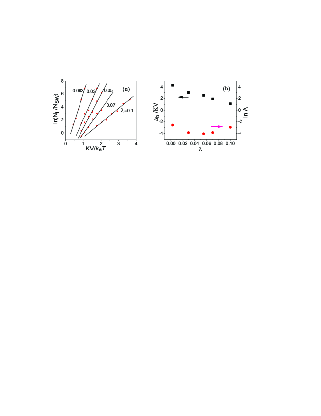
Figure 3: (a) Stochastic simulations of spontaneous Néel vector reversal [$\ln(N_{i}/N_{sw})$] as a function of the inverse temperature for different values of the damping constants $\lambda$. The date points (dots) show the results of the calculation while their exponential approximations are given by the fitted lines. For sufficient statistics, the iterative process based on random Monte Carlo selection continues until the number of observed switching events $N_{sw}$ reaches 150 or more. (b) Effective barrier $\Delta_{b}$ and prefactor $A$ determined from the slopes and the intercepts of the fitted lines shown in (a). Note that $k_{B}T$ and $\Delta_{b}$ are normalized to the anisotropy energy $KV$ at the saddle point (where $K=\left|K_{x}\right|$ and $V$ denotes the AFM nano-particle volume).

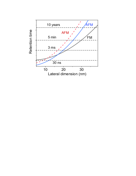
Figure 4: Retention times of AFM and FM nano-particles at room temperature as a function of the lateral dimension. The solid lines represent the cases of uniaxial symmetry (both AFM and FM), while the dashed line is for the biaxial AFM nano-particle ($K_{x}<0$, $K_{z}>0$). A square cross-section is assumed whereas the vertical thickness is fixed at 5 nm.

- (1) D. V. Berkov and N. L. Gorn, J. Magn. Magn. Mater. 272-276, 687 (2004).
- (2) U. Atxitia, O. Chubykalo-Fesenko, R. W. Chantrell, U. Nowak, and A. Rebei, Phys. Rev. Lett. 102, 057203 (2009).
- (3) K. Galatsis, A. Khitun, R. Ostroumov, K. L. Wang, W. R. Dichtel, E. Plummer, J. F. Stoddart, J. I. Zink, J. Y. Lee, Y.-H. Xie, and K. W. Kim, IEEE Trans. Nanotechnol. 8, 66 (2009).
- (4) C. Vogler, C. Abert, F. Bruckner, D. Suess, and D. Praetorius, J. Appl. Phys. 119, 223903 (2016).
- (5) A. Slavin and V. Tiberkevich, IEEE Trans. Magn. 45, 1875 (2009).
- (6) W. F. Brown, Phys. Rev. 130, 1677 (1963).
- (7) C. W. Gardiner, Handbook of stochastic methods for physics, chemistry, and the natural sciences (Springer, Berlin, 2004).
- (8) J.-G. Zhu, in Handbook of magnetism and advanced magnetic materials, eds. H. Kronmüller and S. Parkin (John Wiley, New York, 2007), Chap. 2.
- (9) F. Romá, L. F. Cugliandolo, and G. S. Lozano, Phys. Rev. E 90, 023203 (2014).
- (10) T. Jungwirth, X. Marti, P. Wadley, and J. Wunderlich, Nat. Nano. 11, 231 (2016).
- (11) P. Thibaudeau and S. Nicolis, IEEE Trans. Magn. 52, 1300504 (2016).
- (12) H. V. Gomonay and V. M. Loktev, Eur. Phys. J. Special Topics 216, 117 (2013).
- (13) V. D. Tsiantos, T. Schrefl, W. Scholz, and J. Fidler, J. Appl. Phys. 93, 8576 (2003).
- (14) A. F. Andreev and V. I. Marchenko, Sov. Phys. Usp. 23, 21 (1980).
- (15) B. A. Ivanov and A. K. Kolezhuk, Low Temp. Phys. 21, 760 (1995).
- (16) E. V. Gomonay and V. M. Loktev, Low Temp. Phys. 40, 17 (2014).
- (17) Y. G. Semenov, X.-L. Li, and K. W. Kim, Phys. Rev. B 95, 014434 (2017).
- (18) V. I. Mel’nikov, Phys. Rep. 209, 1 (1991).
- (19) Y. P. Kalmykov, J. Appl. Phys. 96, 1138 (2004).
- (20) V. N. Smelyanskiy, M. I. Dykman, H. Rabitz, and B. E. Vugmeister, Phys. Rev. Lett. 79, 3113 (1997).
- (21) M. I. Dykman, Phys. Rev. A 42, 2020 (1990).
- (22) R. Khymyn, I. Lisenkov, V. Tiberkevich, B. A. Ivanov, and A. Slavin, Sci. Rep. 7, 43705 (2017).
- (23) L. Breth, D. Suess, C. Vogler, B. Bergmair, M. Fuger, R. Heer, and H. Brueckl, J. Appl. Phys. 112, 023903 (2012).
- (24) X.-L. Li, X. Duan, Y. G. Semenov, and K. W. Kim, J. Appl. Phys. 121, 023907 (2017).
- (25) O. Gomonay, T. Jungwirth, and J. Sinova, Phys. Status Solidi RRL 11, 1700022 (2017).
- (26) V. Baltz, A. Manchon, M. Tsoi, T. Moriyama, T. Ono, and Y. Tserkovnyak, Rev. Mod. Phys. 90, 015005 (2018).