A Parsec-scale Bipolar H₂ Outflow in the Massive Star Forming Infrared Dark Cloud Core MSXDC G053.11+00.05 MM1

Abstract

We present a parsec-scale molecular hydrogen (H₂ 1-0 S(1) at 2.12 µm) outflow discovered from the UKIRT Widefield Infrared Survey for H₂. The outflow is located in the infrared dark cloud core MSXDC G053.11+00.05 MM1 at 1.7 kpc and likely associated with two young stellar objects (YSOs) at the center. The overall morphology of the outflow is bipolar along the NE-SW direction with a brighter lobe to the southwest, but the detailed structure consists of several flows and knots. With the total length of $\sim$1 pc, the outflow luminosity is fairly high with $L_{\rm H_{2}}>6~{}L_{\sun}$, implying a massive outflow-driving YSO if the entire outflow is driven by a single source. The two putative driving sources, located at the outflow center, show photometric variability of $\gtrsim$1 mag in H- and K-bands. This, with their early evolutionary stage from spectral energy distribution (SED) fitting, indicates that both are capable of ejecting outflows and may be eruptive variable YSOs. The YSO masses inferred from SED fitting are $\sim$10 $M_{\sun}$ and $\sim$5 $M_{\sun}$, suggesting the association of the outflow with massive YSOs. The geometrical morphology of the outflow is well explained by the lower mass YSO by assuming a single source origin, but without kinematic information, the contribution from the higher mass YSO cannot be ruled out. Considering star formation process by fragmentation of a high-mass core into several lower mass stars, we also suggest the possible presence of another, yet-undetected driving source deeply embedded in the core.

1 Introduction

Outflows and jets from protostars are major outcomes of the star formation process and one of the prominent observational signs in star-forming regions. In low-mass star formation, outflows and jets, driven by magnetic stresses or magneto-centrifugal force in accretion disks, play an important role in removing a large fraction of angular momentum from rotating disks and provide a clue to accretion processes/history of young stellar objects (YSOs) (e.g., Shu et al., 1994; Frank et al., 2014; Caratti o Garatti et al., 2015, and references therein). In high-mass star formation, on the other hand, it is still controversial whether their formation process is a scaled-up version of low-mass star formation (Bonnell et al., 2001; McKee & Tan, 2003; Wang et al., 2010; Tan et al., 2014), and the roles of outflows and jets have thus far remained unclear. Since massive stars are small in number, distant (several kpc), heavily obscured ($A_{\rm V}$ up to 100 mag), and evolve in a short timescale compared to low-mass stars, it is difficult to observationally examine massive star formation process. Because of large extinction, outflows from massive YSOs are not accessible by optical emission lines (e.g., [O I], [S II], H$\alpha$), the outflow-shock tracers frequently used in low-mass YSOs, so they have mainly been explored by molecular lines such as CO or SiO at (sub)millimeter wavelengths (e.g., Beuther et al., 2002; Wu et al., 2005; López-Sepulcre et al., 2009). Those lines from radio observations trace molecular outflows but generally suffer from low spatial resolution except a few interferometer observations. Recently, several surveys of outflows/jets in near-infrared (near-IR), particularly by using the H₂ 1-0 S(1) line at 2.12 µm have been carried out, allowing us to trace shocks in molecular outflows and investigate the primary outflows ejected from their driving sources on scales of a few thousands of AUs to parsecs. Many studies have revealed H₂ outflows from intermediate- or high-mass YSOs some of which are well collimated as outflows from low-mass YSOs, suggesting that disk accretion is likely the leading mechanism in high-mass star formation as well as in low-mass star formation (e.g., Davis et al., 2008, 2010; Varricatt et al., 2010; Lee et al., 2013; Caratti o Garatti et al., 2015).

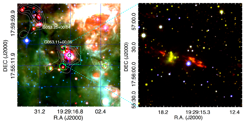
Figure 1: Left: Three-color image of MSXDC G053.11+00.05 produced from Spitzer IRAC 5.8 $\micron$ (B), IRAC 8.0 $\micron$ (G), and MIPS 24 $\micron$ (R) images. White contours are the 1.2 mm continuum emission from the Bolocam Galactic Plane Survey (Aguirre et al., 2011). G53.11_MM1 and the other four cores in MSXDC G053.11+00.05 are marked by black and green circles, respectively. The north-east region is a part of another IRDC MSXDC G053.25+00.04 (Simon et al., 2006). Right: Three-color image of the G53.11_MM1 outflow marked by a cyan dashed-box in the left panel, produced from the UKIRT/WFCAM J(B), K(G), and H₂(R) images.

In this paper, we present a remarkable H₂ outflow and putative outflow-driving YSOs discovered in the infrared dark cloud (IRDC) core MSXDC G053.11+00.05 MM1 (G53.11_MM1 hereafter; Simon et al., 2006; Rathborne et al., 2006) displayed in Figure 1. MSXDC G053.11+00.05 is a part of a long, filamentary CO molecular cloud located at Galactic coordinates $(l,b)\sim(53\fdg 2,0\fdg 0)$, which was defined as IRDC G53.2 in our previous study (see Figure 1 of Kim et al., 2015). The kinematic distance of IRDC G53.2 obtained from the CO line velocity of $\sim$23 km s^-1 is from 1.7 to 2.0 kpc depending on the Galactic rotation model (Rathborne et al., 2006; Ragan et al., 2014; Kim et al., 2015); in this study, we adopt 1.7 kpc derived by using a flat rotation curve with $R_{\sun}=8.5$ kpc and $\Theta_{\sun}=220$ km s^-1 (Kim et al., 2015). IRDC G53.2 is an active star-forming region with more than 300 YSO candidates (Kim et al., 2015) and a large number of molecular hydrogen (H₂ 1-0 S(1) at 2.12 µm) emission-line objects (MHOs) revealed from the UKIRT Widefield Infrared Survey for H₂ (UWISH2; Froebrich et al., 2011, 2015). Among those MHOs identified in IRDC G53.2, the G53.11_MM1 outflow we address here is the most prominent H₂ outflow with a well-defined bipolar morphology (Figure 1) and is rather isolated from the central, crowded region where it is difficult to speculate the driving source. The G53.11_MM1 outflow is likely associated with high-mass star formation as the outflow is found at the center of the IRDC core.

In MSXDC G053.11+00.05, five millimeter cores have been detected (Rathborne et al., 2006) as marked in the left panel of Figure 1. Among them, G53.11_MM1 is the brightest and most massive one with its mass of 124 $M_{\sun}$ derived from the 1.2 mm flux (Rathborne et al., 2006). At the center of the core, the bipolar H₂ outflow oriented in the NE-SW direction is located with two early-class (Class I) YSOs separated by $\sim$8$\arcsec$ (Kim et al., 2015), YSOs that are referred as YSO1 and YSO2 in this study. Besides YSO1 and YSO2, there are about 80 mid-IR sources idetified in the Galactic Legacy Infrared Midplane Survey Extraordinaire (GLIMPSE) Catalog/Archive (Benjamin et al., 2003; Churchwell et al., 2009) around the H₂ outflow, among which 19 sources are detected in all the Spitzer IRAC bands but not detected in the Spitzer MIPS 24 µm band up to 8.4 mag except one source included in Kim et al. (2015). The spectral indices calculated between 2 and 8 µm (Lada, 1987; Greene et al., 1994) mostly classify them as flat spectrum or Class II with a few Class I (Figure 2); the mid-IR colors (Gutermuth et al., 2009) mostly classify them as photospheric sources or Class II. Although these Class I and II YSOs can drive the outflow, the possibility that they are driving the G53.11_MM1 outflow is low because these YSOs are relatively far from the outflow center. Since the outflow is well defined by a bipolar shape, the driving source is likely at the center of the outflow. Therefore, considering the central location as well as the early evolutionary class, we regard YSO1 and YSO2 as the putative driving sources of the G53.11_MM1 outflow.

Toward G53.11_MM1, several maser detections have been previously reported: 22 GHz water maser, 44 and 95 GHz class I methanol masers from the Korean VLBI Network (KVN) observations (Kang et al., 2015); 6.7 GHz class II methanol maser from the MERLIN observations (G53.14+0.07; Pandian et al., 2011). The detected masers with no radio continuum emission at 5 GHz (Urquhart et al., 2009) support star formation activity in early stages; the positional coincidence between the 6.7 GHz methanol maser G53.14+0.07 at ($\alpha_{2000}$, $\delta_{2000}$)= (${\rm 19^{h}29^{m}17\,\fs 581,+17\arcdeg 56\arcmin 23\farcs 21}$) and one of the two central YSOs (YSO1; see Section 5) strongly indicates that this YSO is a high-mass protostellar object. This suggests that either one (or both) of the central YSOs is massive and a possible driving source of the outflow.

In this study, we investigate the characteristics of the G53.11_MM1 outflow and central YSOs using narrow- and broad-band IR imaging observational data. We derive their physical parameters and discuss their properties. In Section 2, we present the observational data used in this study and data reduction process. In Section 3, we present the characteristics of the H₂ outflow by deriving the geometrical/physical parameters, and in Section 4, we search for [Fe II] emission associated with the H₂ outflow. We then move to the central YSOs in Section 5 presenting their photometric variability and spectral energy distribution (SED) analysis. In Section 6, we discuss the origin of the G53.11_MM1 outflow based on the results from the foregoing sections, and we finally summarize and conclude our study in Section 7.

2 Data

2.1 UKIRT/WFCAM Wide-field Images

The outflow in G53.11_MM1 was first identified from the UWISH2 survey. The UWISH2 survey mapped the First Galactic Quadrant ($6\arcdeg\lesssim l\lesssim 65\arcdeg;|b|\lesssim 1\fdg 5$) with the narrow-band filter centered on the H₂ emission line at 2.12 µm using the Wide-Field Camera (WFCAM) at United Kingdom Infrared Telescope (UKIRT) from 2009 July to 2011 August. The WFCAM has four Rockwell Hawaii-II HgCdTe arrays of $2048\times 2048$ pixels and provides $13\farcm 65\times 13\farcm 65$ field-of-view (FOV) images with a pixel scale of $0\farcs 4$. The images are resampled to $0\farcs 2$ in the final stacked images (Froebrich et al., 2011). The IRDC G53.2 region was observed in 2010 and 2011. For continuum subtraction from the narrow-band H₂ images, we used the broad-band K-band images obtained in 2006 from the UKIRT Infrared Deep Sky Survey of the Galactic plane (UKIDSS GPS; Lucas et al., 2008).

We also used the [Fe II] images obtained from the UKIRT Widefield Infrared Survey for Fe⁺ (UWIFE; Lee et al., 2014) to search for [Fe II] emission associated with the H₂ outflow. UWIFE was designed to complement UWISH2 so that it covers the same area with the same instrument as UWISH2 but using the [Fe II] 1.644 µm narrow filter. The UWIFE survey was performed through 2012 and 2013, and the [Fe II] images of the IRDC G53.2 region were taken in 2012. During the observations, we obtained the H-band images as well for continuum subtraction considering possible variations of continuum emission between 2006 (from UKIDSS GPS) and 2012. Details on the UWISH2 and UWIFE surveys are presented in Froebrich et al. (2011) and Lee et al. (2014), respectively.

All WFCAM data were reduced by the Cambridge Astronomical Survey Unit (CASU) as described in detail in Dye et al. (2006); astrometric and photometric calibrations (Hodgkin et al., 2009) were carried out by using the Two Micron All Sky Survey (2MASS) catalogue (Skrutskie et al., 2006). Continuum subtraction from H₂ and [Fe II] narrow-band images was conducted by using H- and K-band images, respectively, as follows. We first re-projected the broad-band image onto the corresponding narrow-band image to align their astrometry. Since the broad- and narrow-band filters have different bandwidths, we also scaled the broad-band image to match the flux of the narrow-band image. Then, we performed point-spread-function (PSF) photometry of each image and removed detected point sources; we finally subtracted the point-source-removed broad-band image from the point-source-removed narrow-band image to remove other extended continuum sources. The above method was developed as a part of the UWIFE data reduction process, and more detailed explanations are given in Lee et al. (2014).

2.2 Subaru/IRCS High-resolution Imaging Observations

We performed near-IR imaging observations of the central part of the G53.11_MM1 outflow with high angular resolution to explore the detailed structures of the outflow and the vicinity of the central YSOs. The observations were conducted on 2012 July 30 UT by using the Infrared Camera and Spectrograph (IRCS; Tokunaga et al., 1998; Kobayashi et al., 2000) on the Subaru telescope in a service mode (ID: S12A0139S; PI: Pyo, T.-S.). Combined with the adaptive optics (AO) system (AO188; Hayano et al., 2010), IRCS provides near-IR (1–5 µm) images with pixel scales of 20 and 52 mas per pixel for the FOV of $21\arcsec\times 21\arcsec$ and $54\arcsec\times 54\arcsec$, respectively. We obtained [Fe II] 1.644 µm, H₂ 2.122 µm, H (centered at 1.63 µm), and K ($K^{\prime}$ centered at 2.12 µm) images toward G53.11_MM1 centered at ($\alpha_{2000},\delta_{2000}$)=(${\rm 19^{h}29^{m}17\,\fs 29,+17\arcdeg 56\arcmin 17\farcs 59}$) with a pixel scale of $0\farcs 052$ (52 mas mode). Total integration times were 4,500 s for narrow-band filters and 300 s for broad-band filters. The AO guide star was at ($\alpha_{2000},\delta_{2000}$)=(${\rm 19^{h}29^{m}16\,\fs 178,+17\arcdeg 56\arcmin 10\farcs 14}$), about 18$\arcsec$ apart from the center of the observed field, and the seeing after AO correction is $0\farcs 17$ at K-band. We reduced the IRCS data with IRAF and IRCS IRAF script package (ircs_imgred) distributed by National Astronomical Observatory of Japan (NAOJ) following the standard procedure including dark subtraction, flat-fielding, median-sky subtraction, dithered image alignment, and image combining. Continuum emission was subtracted from the narrow-band images ([Fe II] and H₂) by using the broad-band images (H and K) with the same method applied for the UKIRT/WFCAM data.

2.3 Gemini/NIRI High-resolution Imaging Observation

We also performed high-resolution K-band imaging observation of the central part of the G53.11_MM1 outflow using the Near Infrared Imager and Spectrometer (NIRI; Hodapp et al., 2003) attached on the Gemini North telescope on 2015 August 29 UT (Program ID: GN-2015B-Q-16; PI: Lee, J.-J.). Among NIRI’s three cameras, we used f/32 camera with the Gemini facility AO system ALTAIR (Christou et al., 2010), which provides a pixel scale of $0\farcs 022$ per pixel and a FOV of $22\arcsec\times 22\arcsec$. We obtained K-band (Kshort filter centered at 2.15µm) images of the central region of the core centered at ($\alpha_{2000},\delta_{2000}$)=(${\rm 19^{h}29^{m}17\,\fs 36,+17\arcdeg 56\arcmin 18\farcs 32}$) and the sky region, where there is no star, for background subtraction with a total integration time of 720 s for each. The AO guide star was the same as the one used in the Subaru/IRCS observations, and the AO-corrected seeing is $0\farcs 12$. Data reduction was done with Gemini IRAF package and the python scripts for cleaning and linearity correction provided from Gemini Observatory, by following the same standard procedure described in Section 2.2.

2.4 Infrared Archival Data

Since G53.11_MM1 has been identified as a point or compact source from near-IR to millimeter, we used mid- and far-IR archival data as complements to investigate the central YSOs. In mid-IR, we used Spitzer IRAC band (3.6, 4.5, 5.8, and 8.0 µm) images from GLIMPSE (Benjamin et al., 2003; Churchwell et al., 2009) with the GLIMPSE I v2.0 Catalog/Archive, Spitzer MIPS 24 µm image from MIPS GALactic plane survey (MIPSGAL; Carey et al. 2009), and Wide-field Infrared Survey Explore (WISE; Wright et al., 2010) all-sky data. In Spitzer images, two YSOs separated by $\sim$8$\arcsec$ (Kim et al., 2015) are resolved but saturated in the MIPS 24 µm image; in the WISE images, two YSOs are not resolved because of low angular resolution. In far-IR, we used the Herschel Infrared Galactic Plane Survey (Hi-GAL; Molinari et al., 2010) data and the catalog of the IRDC-associated starless and protostellar clumps with known distance in the Galactic longitude range $15\arcdeg\leq l\leq 55\arcdeg$ from Hi-GAL (Traficante et al., 2015) to extract the PACS 70 µm flux of G53.11_MM1.

3 Characteristics of the H₂ Outflow

3.1 H₂ Outflow Morphology

3.1.1 Identification of H₂ Emission

Figure 2 presents the UKIRT/WFCAM H₂ image of the G53.11_MM1 outflow before (top) and after (bottom) continuum subtraction. The overall morphology of the outflow is bipolar but is composed of several discrete flows and knots. We identified the H₂ emission features of the outflow to derive their geometrical parameters and H₂ line flux. In the continuum-subtracted image, we estimated the background value ($F_{bg}$) and determined a threshold for the outflow emission as three sigma above the background ($F_{bg}+3\sigma\simeq 2.9\times 10^{-20}~{}{\rm W\,m^{-2}}$). In the bottom panel of Figure 2, red contours are 1$\sigma$, 3$\sigma$, 10$\sigma$, 45$\sigma$, and 80$\sigma$ above the background, and the thick contours ($=F_{bg}+3\sigma$) present the threshold, which is also drawn by red contours in the top panel of the figure. In this process, we excluded artifacts and emission features with the area smaller than $<$0.25 arcsec² (i.e., the area of a circle with its diameter of 1$\arcsec$) considering that a typical full width half maximum of the stellar PSF of the UWISH2 data is $<$1$\arcsec$ (Ioannidis & Froebrich, 2012a). In total, we identified 13 H₂ emission features and assigned the numbers from #1 to #8; for the flows/knots in the same direction, we grouped them and assigned the same numbers with different alphabets (e.g., from #2a to #2c, and from #3a to #3d) as shown in the top panel of Figure 2.

Since the H₂ emission defined by the contours at the threshold has irregular shapes, we fitted the individual emission features by an ellipse to derive their geometrical parameters. For the fitting, we used the IDL procedure FIT_ELLIPSE included in the Coyote IDL Program Libraries. The fitting results are drawn as black dashed ellipses in the top panel of Figure 2, and the derived geometrical parameters are presented in Table 1. The central coordinate, size, and orientation angle ($\psi_{\rm ellipse}$) of the H₂ emission features have been derived by adopting the center position, length of major axis, and orientation angle (from north to east) of the major axis of the fitted ellipses, respectively. The position angles (PAs) PA1 and PA2 have been measured by the angle (from north to east) of the central position of the emission features with respect to YSO1 and YSO2, respectively, because the driving source is not clearly known (see Section 3.1.4). Table 1 also lists the area and H₂ line flux (see Section 3.2) of the emission features that have been directly estimated from their contours.

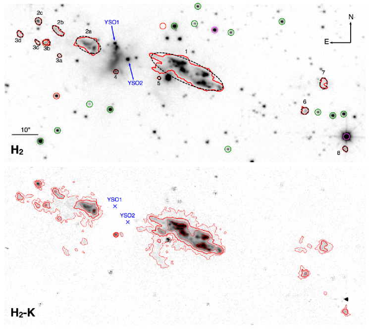
Figure 2: Top: UKIRT/WFCAM H₂ image of the G53.11_MM1 outflow. Red contours present the individual emission features defined by the threshold of three sigma above the background (thick contours in bottom panel), and black dashed ellipses are the results of the ellipse fitting of each contour. Two YSOs at the center (YSO1 and YSO2) are marked. Circles identify the mid-IR sources from GLIMPSE catalog/archive: red, green, magenta colors indicate Class I, Class II including flat spectrum, and Class III YSOs defined by the spectral indices calculated between 2 and 8 µm. Bottom: The continuum-subtracted H₂ image. Red contours are $1\sigma,3\sigma,10\sigma,45\sigma$, and $80\sigma$ above the background. The thick red contours ($3\sigma$) present the threshold used for the identification of the H₂ outflow emission features.

Table 1: Physical Parameters of the H₂ Emission Features of the G53.11_MM1 Outflow

ID	R.A. (J2000)	Dec (J2000)	Size	Size	$\psi_{\rm ellipse}$	PA1	PA2	Area	Line Flux	UWISH2 Source ID
			(arcsec)	(pc)	(deg)	(deg)	(deg)	(arcsec2)	($10^{-18}$ ${\rm W\,m}^{-2}$)
1	19:29:15.68	17:56:12.6	59.0	0.97	65	69	78	179.2	1063.0	UWISH2_053.13615+0.07569
2a	19:29:18.31	17:56:22.7	19.7	0.32	65	$\cdots$	70	39.9	137.9	UWISH2_053.14447+0.06663
2b	19:29:19.11	17:56:28.0	11.1	0.18	47	$\cdots$	68	8.3	13.7	UWISH2_053.14447+0.06663
2c	19:29:19.63	17:56:31.7	5.7	0.09	25	$\cdots$	67	5.1	18.1	UWISH2_053.14796+0.06517
3a	19:29:19.07	17:56:18.6	3.1	0.05	42	$\cdots$	87	1.7	2.4	UWISH2_053.14447+0.06663
3b	19:29:19.42	17:56:23.6	5.6	0.09	73	$\cdots$	78	4.4	7.3	UWISH2_053.14447+0.06663
3c	19:29:19.66	17:56:23.6	5.1	0.08	40	$\cdots$	79	2.2	2.4	UWISH2_053.14447+0.06663
3d	19:29:20.12	17:56:26.8	5.6	0.09	37	$\cdots$	77	3.8	4.5	UWISH2_053.14447+0.06663
4	19:29:17.57	17:56:12.6	3.7	0.06	80	2	137	2.4	7.9	$\cdots$
5	19:29:16.43	17:56:10.2	2.5	0.04	35	52	59	1.2	1.1	UWISH2_053.13615+0.07569
6	19:29:12.56	17:55:57.7	5.6	0.09	137	70	74	5.4	9.1	UWISH2_053.12637+0.08503
7	19:29:12.06	17:56:08.1	8.6	0.14	0	79	83	7.6	8.3	UWISH2_053.12785+0.08817
8	19:29:11.48	17:55:43.3	4.5	0.07	29	65	68	2.8	4.3	UWISH2_053.12064+0.08683
Total	$\cdots$	$\cdots$	126	1.04	$\cdots$	67	74	264	1280	$\cdots$

Note. — R.A. (J2000), Dec (J2000) = central coordinates derived from the center of the fitted ellipses; Size and $\psi_{\rm ellipse}$ = length and orientation angle (from north to east) of the major axis of the fitted ellipses; PA1 and PA2 = position angle (from north to east) of the emission features with respect to YSO1 and YSO2 (see Section 3.1.4); Area = area of the individual contours; Line Flux = H₂ line flux directly measured from the individual contours with the uncertainty of $\sim$10%; UWISH2 Source ID = from the UWISH2 extended H₂ source catalog (Froebrich et al., 2015).

3.1.2 Apparent Morphology

The outflow can be divided into the main flow (from #1 to #5) and the faint knots (from #6 to #8) in the southwest. The main outflow has a bipolar shape along the NE-SW direction. While the NE flow is made up of two groups of flows (#2 and #3), the SW flow is identified as one flow (#1) because the whole flow is brighter than the threshold. This brightness difference between the two flows implies that the brighter SW flow is likely blueshifted if both flows originate from a single source.

The flow #1 is composed of several, at least six bright flows and knots as shown by the contours at the higher levels than the threshold in the bottom panel of Figure 2; the faint emission #5 also can be a part of #1. The sub-flows in #1 have slightly different orientations and show a bow-shock-like feature at their tips (see Figure 8 for higher-resolution images). The flow #2a consists of two components: a compact knot and a flow with a bow-shock-like tip that is well connected to the flows #2b and #2c. The emission features grouped as #3 are smaller and fainter than those in #2. As shown by the one-sigma level contours in the bottom panel of Figure 2, #2 and #3 have different orientations from the outflow center, and #3a is not well aligned with the other knots in #3. The complicated structure with several flows of different orientations seen in the flows #1, #2, and #3 may imply multiple precessing jets; we discuss this possibility in detail in Section 6. The emission #4 is near the center of the main flow, at the southern end of the central nebula. Since #4 is detected in both UKIRT and Subaru images, it is not residual nebula emission from continuum subtraction but real H₂ emission. The association between #4 and the other H₂ features of the outflow is ambiguous because the direction from the central YSOs to #4 is almost perpendicular to the whole outflow in the NE-SW direction, raising a question whether #4 is a part of another, separate outflow (see Section 6).

The remaining emission features #6, #7, and #8 located in the southwest are faint but clearly seen in the continuum-subtracted image. They are rather far away, but there is no other YSO or other object that can emit H₂ emission, indicating their association with the main flow. We note that we have found faint emission features on the opposite side as well, i.e., toward the northeast, outside the region shown in Figure 2, at a similar distance to #8 from the outflow center; however, it is unclear whether they are associated with G53.11_MM1 because their surroundings are complicated, with another H₂ emission features and YSO candidates, so we do not include them in this study and only consider the H₂ emission presented in Figure 2, i.e., from #1 to #8.

3.1.3 Size and Mass Ejection Frequency

Size of the individual H₂ emission features of the outflow estimated from the major axis of the fitted ellipses is from 3$\arcsec$ to $\sim$60$\arcsec$ typically with the larger size for the brighter ones (Table 1). The total length of the outflow is $\sim$80$\arcsec$ if only the main flow from #1 to #5 is considered, or $\sim$130$\arcsec$ if the faint knots in the southwest (#6, #7, #8) are included, corresponding to $\sim$0.7 and $\sim$1 pc, respectively, at the distance to IRDC G53.2, 1.7 kpc. From the length of the one lobe (the SW lobe), from 0.35 to 0.74 pc, we constrain the dynamical age of the outflow, although it gives a wide range of timescales depending on the outflow velocity and inclination with respect to the plane of the sky: from 16,000 to 36,000 yr with the velocity of 20 km s^-1; from 3,000 to 7,200 yr with the velocity of 100 km s^-1. The assumed velocity range from 20 to 100 km s^-1 is adopted from the observed proper motions of H₂ outflows (Khanzadyan et al., 2003; Raga et al., 2013), but we note that an outflow velocity can be as high as 150–300 km s^-1 (e.g., Bally et al., 2015). While protostellar outflows from low-mass YSOs are typically in sub-parsec scale with a small ($\sim$10%) fraction of parsec scale outflows (Stanke et al., 2002; Davis et al., 2008, 2009; Ioannidis & Froebrich, 2012a), the outflows from high-mass YSOs tend to be more spatially extended (Varricatt et al., 2010; Caratti o Garatti et al., 2015). Thus, the relatively large ($\sim$1 pc) size of the G53.11_MM1 outflow suggests that the outflow-driving source is likely massive.

As described above, the outflow is composed of several flows and knots. The discrete components or clumpy features are often interpreted as episodic mass ejection (Dunham et al., 2014, and references therein), so we measured the separations between the emission features that are well aligned in order to examine the mass ejection frequency. The separations between the knots in the main flow are typically around 10$\arcsec$: the separations between #2a and #2b, between #2b and #2c, and between #3b and #3d by assuming YSO2 as a driving source. The separation between two sub-knots in #1 (sub2 and sub5 in Figure 8) along the line from YSO2 is also $\sim$10$\arcsec$. The separation of 10$\arcsec$ corresponds to a time gap about 1,000 yr with the outflow velocity of 80 km s^-1. (Here, we assume the outflow velocity to be the same as the velocity assumed in two studies using the same UWISH2 data for comparison; Ioannidis & Froebrich 2012b, Froebrich & Makin 2016.) This time gap of $\sim$1,000 yr is comparable to the typical time gaps between the H₂ knots of the outflows in Serpens/Aquila (1,000–2,000 yr; Ioannidis & Froebrich, 2012b) and Cassiopeia/Auriga (1,000–3,000 yr; Froebrich & Makin, 2016). The separations to the faint knots in the southwest are larger: the separations between the southernmost sub-knot in #1 (sub1 in Figure 8) and #8 along the line from YSO1 is $\sim$60$\arcsec$; the separation between the same knot and #6 along the line from YSO2 is $\sim$40$\arcsec$. These large separations may imply that the distant, faint knots are not a part of the G53.11_MM1 outflow or that we have missed much fainter emission between them, but it is also possible that the mass ejection frequency and/or outflow velocity is not constant over time or that multiple jets with different direction and velocity have been explosively ejected.

3.1.4 Position Angle

We present the PAs of the H₂ emission features in Table 1. Since the outflow-driving source is unknown, we separately measured PAs of the emission features with respect to YSO1 and YSO2 from north to east, and defined them as PA1 and PA2, respectively. For YSO1, we only consider the emission in the southwest (#1, #5, #6, #7, #8) because the NE flow requires a high degree of precession if it has been ejected from YSO1; for YSO2, we consider all of the emission features except #4 that has a different PA as described in Section 3.1.2. The measured PAs of the emission features with respect to YSO1 (PA1) are from 52$\arcdeg$ to 79$\arcdeg$ with the mean of $67\arcdeg^{+12}_{-15}$, and the PAs with respect to YSO2 (PA2) are from 59$\arcdeg$ to 87$\arcdeg$ with the mean of $74\arcdeg^{+13}_{-15}$. The accurate PA of the entire outflow can be measured once the driving source is confirmed, but our current results indicate that in any case, the PA will be around 70$\arcdeg$. Table 1 also shows that the PA of #4 is indeed very different from those of the other features as expected—the estimated PAs are 2$\arcdeg$ and 137$\arcdeg$ with respect to YSO1 and YSO2, respectively.

3.2 H₂ Outflow Luminosity

We derived the H₂ luminosity of the G53.11_MM1 outflow from the UWISH2 image. We first estimated the H₂ 1-0 S(1) emission line flux ($F_{2.12}$) given as $F_{2.12}=F_{0}({\rm DN}/t_{\rm exp})10^{-0.4ZP}$ from the continuum-subtracted image, where $F_{0}$ ($=9.84\times 10^{-12}$ ${\rm W\,m}^{-2}$) is a total in-band flux of the H₂ filter, DN is the total sum of pixel values of the region of interest, $t_{\rm exp}$ is the exposure time ($=60$ s), and $ZP$ is the zero-point magnitude ($=21.125$ mag for our image) written in the image header. Calculating the total sum of pixel values, we multiplied a factor of 1.10 in order to compensate the H₂ line flux that is included in the K-band image so subtracted during the continuum-subtraction process (Lee, Y.-H. et al. in preparation). With the uncertainty of $\sim$10% in flux measurements, the estimated 2.12 µm line flux of each contour determined in Section 3.1.1 is from $1.1\times 10^{-18}$ to $1063.0\times 10^{-18}$ ${\rm W\,m}^{-2}$ as listed in Table 1, giving the total line flux of $1.28\times 10^{-15}$ ${\rm W\,m}^{-2}$ for the total area of 264 arcsec². We note that the threshold we used to identify the H₂ emission features, three sigma above the background, is rather conservative, so our flux estimation gives a lower limit. For comparison, the G53.11_MM1 outflow is also included in the UWISH2 extended H₂ source catalog (Froebrich et al., 2015) as we present the UWISH2 source IDs in the last column of Table 1. The contours of the UWISH2 sources corresponding to the G53.11_MM1 outflow are almost consistent with the contours at the level of one sigma above the background in Figure 2 (bottom), enclosing the area about three times larger than our results. The different threshold values, however, insignificantly affect the total line flux because most of the additional area have very low surface brightness. The H₂ line flux of the G53.11_MM1 outflow region from the UWISH2 catalog (Froebrich et al., 2015) is $\sim$10% larger than our estimation.

From the total 2.12 µm line flux $F_{\rm 2.12,obs}\sim 1.28\times 10^{-15}$ ${\rm W\,m}^{-2}$, the 2.12 µm luminosity of the outflow at the distance of 1.7 kpc is $L_{\rm 2.12,obs}\sim 0.1~{}L_{\sun}$, but this is highly underestimated because extinction toward IRDC cores is expected to be large. Since the extinction of G53.11_MM1 has not been previously measured, we constrain the lower and upper limits using the optical depth of the Spitzer dark cloud SDC053.158+0.068 (Peretto & Fuller, 2009) and the ¹³CO column density $N(^{13}{\rm CO})$ obtained from the ¹³CO $J=$ 1–0 data in the Boston University-Five College Radio Astronomy Observatory Galactic Ring Survey (GRS; Jackson et al., 2006), respectively. SDC053.158+0.068 is a large (major axis $\sim 300\arcsec$) dark cloud that includes G53.11_MM1. The averaged optical depth of SDC053.158+0.068 measured at 8 µm is 0.68, or $A_{\rm 8\mu m}=0.63$ mag (Peretto & Fuller, 2009). The extinction $A_{\rm 8\mu m}=0.63$ mag is converted to $A_{K}\sim 1.5$ mag or $A_{\rm V}\sim 15$ mag by the mid-IR extinction curves derived in Flaherty et al. (2007) and Chapman et al. (2009); this value $A_{\rm V}\sim 15$ mag can be the lower limit of the extinction of G53.11_MM1, a denser core inside the dark cloud. In our previous study, we derived the $N(^{13}{\rm CO})$ map of IRDC G53.2 from the GRS ¹³CO $J=$ 1–0 data (Kim et al., 2015). In the GRS column density map with a large angular resolution (46$\arcsec$) and pixel scale (20$\arcsec$), G53.11_MM1 is covered by a few pixels with $N(^{13}{\rm CO})$ around $9\times 10^{16}$ cm^-2. From $N(^{13}{\rm CO})$, we derive $N_{\rm H_{2}}$ assuming the same numbers of ${}^{12}{\rm CO}/^{13}{\rm CO}=60$ (Equation (3) of Milam et al., 2005) and $n(^{12}{\rm CO})/n({\rm H_{2}})=1.1\times 10^{-4}$ (Pineda et al., 2010) used to derive the $N(^{13}{\rm CO})$ map (Section 2 of Kim et al., 2015). The derived $N_{\rm H_{2}}$ is $\sim 5\times 10^{22}$ cm^-2, or $A_{\rm V}\sim 50$ mag. Since the extinction value derived from $N(^{13}{\rm CO})$ takes the entire thickness of the molecular cloud along the line of sight into account, we adopt $A_{\rm V}=50$ mag as the upper limit of the extinction of G53.11_MM1. From the above, the extinction of G53.11_MM1 is 15 mag $<A_{\rm V}<$ 50 mag, leading to the extinction-corrected 2.12 µm luminosity of the outflow $0.4<L_{\rm 2.12}/L_{\sun}<10$. Then, we derive the total H₂ luminosity ($L_{\rm H_{2}}$) applying the ratio between the 2.12 µm intensity ($I_{2.12}$) and the total H₂ intensity ($I_{\rm H_{2}}$). While the assumption $I_{2.12}/I_{\rm H_{2}}\sim 0.1$ is commonly used (e.g., Stanke et al., 2002; Caratti o Garatti et al., 2006; Ioannidis & Froebrich, 2012b), $I_{2.12}/I_{\rm H_{2}}$ is in fact a function of gas temperature in LTE conditions. We assume the gas temperature of 1,500–3,000 K, although the temperatures of outflows from high-mass YSOs tend to be relatively higher ($\sim$2,500 K; Smith et al., 1997; Davis et al., 2004; Caratti o Garatti et al., 2015), and apply $I_{2.12}/I_{\rm H_{2}}$ of 0.1–0.05 (Figure 3 of Caratti o Garatti et al., 2006). The $L_{\rm H_{2}}$ of the G53.11_MM1 outflow finally derived in the constrained ranges of extinction and temperature is, therefore, $6\pm 2<L_{\rm H_{2}}/L_{\sun}<150\pm 50$.

In several studies, the H₂ luminosity of outflows shows a strong correlation with the bolometric luminosity ($L_{\rm bol}$) of the driving sources (e.g., Caratti o Garatti et al., 2006; Cooper et al., 2013; Caratti o Garatti et al., 2015), thus we can constrain the driving source of the G53.11_MM1 outflow from the derived outflow luminosity. The luminosities of the outflows driven by low-mass YSOs are typically lower than the luminosity of the G53.11_MM1 outflow. For example, $L_{\rm H_{2}}$ of 23 protostellar jets driven by low- and intermediate-mass YSOs studied in Caratti o Garatti et al. (2006) ranges from 0.007 to 0.76 $L_{\sun}$; the outflows detected in Serpens/Aquila from the UWISH2 survey show $L_{\rm H_{2},obs}$ ranging from 0.01 to 1.0 $L_{\sun}$, which is less than a few solar luminosity after extinction correction by using a typical extinction of the region, $A_{K}=1$ mag (Ioannidis & Froebrich, 2012b). The driving source of the G53.11_MM1 outflow, therefore, is expected to be a high- or at least intermediate-mass YSO. We further constrain $L_{\rm bol}$ of the driving source by adopting the empirical relationship between $L_{\rm H_{2}}$ of the outflows and $L_{\rm bol}$ of the protostars derived from the excitation conditions and visual extinction values obtained by spectroscopic observations, a relationship that is defined as $L_{\rm H_{2}}\propto L_{\rm bol}^{\alpha}$ with $\alpha=0.59$ or $\alpha=0.57\sim 0.62$ for outflows from very young (Class 0 and Class I) low-mass or high-mass YSOs, respectively (Figure 9 of Caratti o Garatti et al., 2015). On the relation of $L_{\rm H_{2}}\propto L_{\rm bol}^{\alpha}$ with $\alpha\sim 0.6$, the $L_{\rm bol}$ of the driving source expected from the outflow luminosity $6\pm 2<L_{\rm H_{2}}/L_{\sun}<150\pm 50$ is $\sim 10^{4}<L_{\rm bol}/L_{\sun}<10^{6}$, supporting a high-mass protostar as a driving source of the G53.11_MM1 outflow.

Although the rough information on the environmental conditions such as visual extinction or gas temperature provides a wide range of the H₂ luminosity of the G53.11_MM1 outflow, the constrained $L_{\rm bol}$ suggests that the G53.11_MM1 outflow is likely driven by a high-mass YSO. However, we note that we have assumed a single source origin for the entire H₂ emission in the above discussion, leaving a possibility of multiple outflow-driving YSOs with lower luminosity/mass, which will be discussed in Section 6.

4 Search for [Fe II] Emission in G53.11_MM1

[Fe II], together with H₂, is one of the prominent emission lines tracing protostellar jets. In outflows/jets with H₂ emission, [Fe II] emission, in particular the [Fe II] 1.644 µm lines in near-IR, are frequently observed as well regardless of mass and evolutionary stage of the exciting stars (e.g., Reipurth et al., 2000; Nisini et al., 2002; Giannini et al., 2004; Caratti o Garatti et al., 2006, 2015; Cooper et al., 2013), although the detection rates, morphologies, and spatial distributions are different because these two lines arise from different shock origins: H₂ lines trace slow and non-dissociative shocks whereas [Fe II] lines trace fast and dissociative shocks (Nisini et al., 2002; Hayashi & Pyo, 2009). Since the G53.11_MM1 outflow is strong and well-defined by a bipolar shape in H₂, it can be expected that [Fe II] emission is also observed as a narrow jet emitted from the central YSOs as seen in a number of Herbig-Haro (HH) objects (e.g., HH 300, HH 111; Reipurth et al., 2000) or as compact knots (e.g., HH 223: López et al. 2010; G35.2N: Lee et al. 2014).

We searched for [Fe II] 1.644 µm emission associated with the G53.11_MM1 outflow. We found no [Fe II] emission in the UWIFE image with a typical root-mean-square noise level of $8.1\times 10^{-20}$ ${\rm W\,m^{-2}\,arcsec^{-2}}$ (Lee et al., 2014) but detected faint emission features in the Subaru/IRCS image owing to the higher sensitivity. As the Subaru/IRCS images in Figure 3 show, the [Fe II] emission was found around the sub-flows in the H₂ flow #1 (sub4 and sub5 in Figure 8). The right panel of Figure 3 is the continuum-subtracted [Fe II] image in the inverted-gray color scale with the [Fe II] emission drawn by green contours. Since the background is very noisy and the [Fe II] emission features are barely seen even in the continuum-subtracted image, we smoothed the image by a Gaussian function with three pixels. In the figure, the green contours represent three- and six-sigma above the background estimated from the smoothed image, the negative features seen in white are the H₂ lines included in H-band that have remained after continuum subtraction, and red dashed lines are the H₂ 2.12 µm contours drawn for comparison.

The detected [Fe II] emission is very small with the total length of $\sim$3$\arcsec$ (or the area of $\sim$1 arcsec²) and faint; the three-sigma flux of the [Fe II] line is $\sim 5.7\times 10^{-19}$ ${\rm W\,m}^{-2}$ with the uncertainty of 10%, or the surface brightness is $\sim 5.6\times 10^{-19}$ ${\rm W\,m^{-2}\,arcsec^{-2}}$, which is $<$10% of the surface brightness of the H₂ emission estimated as $\sim 4.8\times 10^{-18}$ ${\rm W\,m^{-2}\,arcsec^{-2}}$ from the total H₂ line flux and area (Table 1). Although the [Fe II] emission is spatially coincident with the H₂ emission, it is difficult to conclude that the [Fe II] emission is associated with the H₂ outflow because [Fe II] knots are generally expected to be observed at the tips of the H₂ bow shocks, where the shock velocities are high and the gas will be dissociated, rather than behind the H₂ bow shocks (e.g., Davis et al., 1999, 2000; López et al., 2010; Lee et al., 2014; Bally et al., 2015).

Detection of further [Fe II] emission in G53.11_MM1 with high signal-to-noise ratio requires deeper imaging observations, but the marginal detection of [Fe II] emission can be interpreted as intrinsically fainter or absent [Fe II] emission compared to H₂ emission. In the outflows from high-mass YSOs, the [Fe II] detection rate with respect to the H₂ detection rate tends to be low, $\lesssim$50% or much less (Cooper et al., 2013; Wolf-Chase et al., 2013; Caratti o Garatti et al., 2015); the brightness of [Fe II] lines also tend to be weaker than the brightness of H₂ lines (Caratti o Garatti et al., 2015). This can be attributed by different extinction effect between the two lines, but more likely, it is because H₂ and [Fe II] emission arise from different physical conditions such as gas density, temperature, or shock velocity. In the G53.11_MM1 outflow, the strong, extended H₂ emission with very weak or negligible [Fe II] emission may imply that slow, C-type shocks are dominant in G53.11_MM1. Further spectroscopic observations will be necessary in order to derive the physical conditions of environment and confirm shock properties.

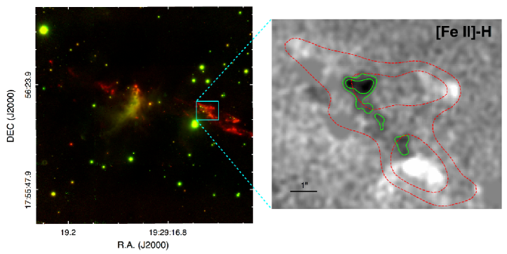
Figure 3: Left: Subaru/IRCS image of G53.11_MM1. Red is H₂, and green is [Fe II]. The cyan box marks the region where the [Fe II] emission features are detected. Right: The continuum-subtracted [Fe II] image of the cyan-box region in the inverted-gray color scale. The image is smoothed by using a Gaussian function, and the residual features from point source subtraction are masked to clearly show the [Fe II] emission. Green contours are the detected [Fe II] emission with the contour levels of $3\sigma$ ($5\times 10^{19}~{}{\rm W\,m^{-2}\,arcsec^{-2}}$) and $6\sigma$ ($9\times 10^{19}~{}{\rm W\,m^{-2}\,arcsec^{-2}}$) above the background estimated from the smoothed image. Red dashed contours are the H₂ emission ($45\sigma$ and $80\sigma$ above the background in Figure 2) drawn for comparison. The negative extended features shown in white are residual H₂ line emission included in H-band that have remained after continuum subtraction.

5 Central Young Stellar Objects

The core G53.11_MM1 is bright from IR to millimeter with large IR-excess emission. The central star (YSO1) was previously identified in the Red MSX Source (RMS) survey with the bolometric luminosity of (3–4)$\times 10^{3}~{}L_{\sun}$ (G053.1417+00.0705; Mottram et al., 2011; Lumsden et al., 2013), but it is in fact composed of two sources, YSO1 and YSO2, separated by $\sim$8$\arcsec$ in the Spitzer mid-IR images with higher spatial resolution. Both YSOs are saturated in the MIPS 24 µm image, but their SEDs with strong excess in mid-IR and spectral indices derived by using the available photometry from the GLIMPSE and MSX catalogs classify them as Class I YSOs that have a dusty envelope infalling onto a central protostar (Kim et al., 2015). The two YSOs are observed in near-IR wavebands as well. Both are fairly bright in K-band, marginally detected in H-band but not observed in J-band, indicating that they are deeply embedded. The evolutionary stages of the YSOs, with the proximity to the center of the outflow (see Figure 2), suggest that one of them or both can be the driving source of the G53.11_MM1 outflow. The coordinates of YSO1 and YSO2 are ($\alpha_{2000},\delta_{2000}$)= (${\rm 19^{h}29^{m}17\,\fs 60,+17\arcdeg 56\arcmin 23\farcs 3}$) and ($\alpha_{2000},\delta_{2000}$)= (${\rm 19^{h}29^{m}17\,\fs 26,+17\arcdeg 56\arcmin 17\farcs 3}$), respectively. Below, we will discuss their photometric variability in near-IR and physical parameters constrained from SED analysis.

5.1 Near-IR Photometric Variability

YSOs are known to commonly show variability (e.g., Carpenter et al., 2001, 2002; Morales-Calderón et al., 2011; Johnstone et al., 2013; Wolk et al., 2013; Rebull et al., 2015). Since we have several H- and K-band images of the central part of G53.11_MM1 obtained at different epochs between 2006 and 2015, we compare the brightness of YSO1 and YSO2 over time. We exclude the 2MASS images in which both YSOs are not clearly resolved and likely contaminated by bright emission of the extended, central nebula due to low resolution. In H-band, we have the UKIRT images taken in 2006 and 2012, and the Subaru/IRCS image taken in 2012; in K-band, we have the UKIRT, Subaru/IRCS, and Gemini/NIRI images obtained in 2006, 2012, and 2015, respectively. Both the UKIRT and Subaru H-band images in 2012 were obtained in July, so we only use the UKIRT image for consistency with the 2006 data. The images are compared in Figure 4. The Subaru and Gemini images with higher resolution show a more complex structure of the central nebula, and variations in relative brightness between YSO1 and YSO2 are seen in some images, e.g., the K-band images between 2012 and 2015.

We estimated the flux of YSO1 and YSO2 from each image. For the UKIRT images, we performed PSF photometry of the point sources using starfinder (Diolaiti et al., 2000) based on the 2MASS catalog (Skrutskie et al., 2006). For the Subaru and Gemini images, we applied differential photometry using the point sources identified in the UKIRT images because our interest is photometric variability of the YSOs. We used four stars without IR excess marked in Figure 4 as reference stars. Table 2 lists the estimated magnitudes of YSO1, YSO2, and the reference stars, and Figure 5 compares the magnitudes of the two YSOs over time. Photometric errors from starfinder are negligibly small but highly underestimated because it only accounts for the errors from PSF fitting and does not include other possible uncertainties such as the uncertainty from background variations that mostly contribute to photometric uncertainties, in particular around the region with nebula emission. In Table 2, the magnitudes of the reference stars at different epochs show the uncertainties less than or around 10%, so we adopt the photometric errors of $\lesssim$10%. We note that S2 exceptionally shows a large difference of $\sim$25% between 2006 and 2012/2015 in K-band. This large uncertainty is likely because S2 is located so close to the nebula that it is more affected by the extended nebula emission particularly in the UKIRT image with lower resolution than in the other two images; if the PSF baseline of S2 in the UKIRT image were determined on the level of the nebula emission, the source flux could have been underestimated from the higher baseline, resulting in the fainter brightness of S2.

Table 3 presents the amplitudes of variability in YSO1 and YSO2 between two time durations: from 2006 to 2012 and from 2012 to 2015. While the variability of YSO2 is obvious in both time durations with magnitude differences of $\gtrsim$1 mag in both H- and K-bands, the variability of YSO1 is rather ambiguous. In H-band, YSO1 was not detected in 2006 but appeared in 2012, giving the magnitude difference larger than 0.76 mag from the detection limit 18.75 mag of the UKIRT H-band image (Lucas et al., 2008); in K-band, however, YSO1 maintained its brightness within the photometric uncertainty between 2006 and 2012. This discrepancy can be also explained by the contamination from the central nebula, but in a manner opposite to S2, the nebula emission could have been included in the source flux since YSO1 is located at the tip of the nebula as seen in Figure 4, leading to overestimation of the K-band flux of YSO1 in 2006. It is less probable that the H-band flux is over/underestimated because the nebula emission in H-band is not as strong as in K-band. We also note that the flux of YSO1 estimated from the Subaru H-band image agrees well with that of the UKIRT image in the same year 2012. Since the two H-band images in Figure 4 were obtained with the same telescope and the same instrument, we believe that the H-band magnitudes in Table 2 are reliable. If assuming that the K-band flux in 2006 is overestimated, YSO1 in 2006 could have been fainter than presented in Table 2 and become brighter in 2012, consistent with the photometric behavior in H-band. The variability of YSO1 is also supported by the brightness change between the 2012 and 2015 K-band images in which the nebula contamination is likely insignificant owing to their higher resolution.

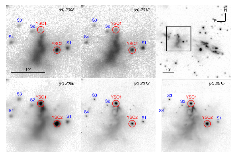
Figure 4: H- and K-band images of the central part of G53.11_MM1 obtained at different epochs. The H₂ image from UWISH2 at the rightmost in upper panel shows the region of interest with a black box. In the rest five figures, the observed bands and years are presented in the right upper side. Two H-band images and the 2006 K-band image were obtained by UKIRT, whereas the K-band images in 2012 and 2015 were obtained by Subaru/IRCS and Gemini/NIRI, respectively. YSO1, YSO2, and the reference stars (from S1 to S4) used for differential photometry are also marked.

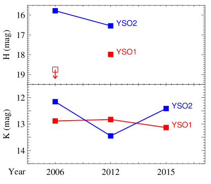
Figure 5: H- and K-band magnitudes of YSO1 and YSO2 over time. Open symbol with an arrow presents the upper limit of YSO1 (=18.75 mag) in the UKIRT H-band image adopted from the typical 90 per cent completeness limit of UKIDSS GPS estimated in uncrowded fields (Lucas et al., 2008). Photometric errors ($\lesssim 10\%$) are smaller than the symbol size.

Table 2: H- and K-band Magnitudes of YSO1, YSO2, and Reference Stars

			H-band (mag)			K-band (mag)
	R.A. (J2000)	Dec(J2000)	UKIRT2006	UKIRT2012		UKIRT2006	Subaru2012	Gemini2015
YSO1	19:29:17.60	17:56:23.3	$>$18.75	17.99		12.88	12.83	13.13
YSO2	19:29:17.26	17:56:17.3	15.78	16.54		12.15	13.45	12.41
S1	19:29:17.04	17:56:17.8	16.51	16.54		14.35	14.34	14.34
S2	19:29:17.79	17:56:22.8	17.91	17.92		15.47	15.23	15.24
S3	19:29:18.05	17:56:24.5	18.06	18.20		14.94	15.09	15.13
S4	19:29:18.22	17:56:19.5	17.26	17.44		15.04	15.10	$\cdots$

Note. — Photometric errors are $\lesssim$10%.

Table 3: Amplitudes of Variability and Colors of YSO1 and YSO2

	$\Delta H_{\rm 2012-2006}$	$\Delta K_{\rm 2012-2006}$	$\Delta K_{\rm 2015-2012}$	$\Delta[H-K]_{\rm 2012-2006}$
YSO1	$<-0.76$	$-0.05$	0.3	$<-0.71$
YSO2	0.76	1.3	$-1.04$	$-0.54$

Flux measurement confirms the variability of both YSOs with the variances up to 0.76 mag in H-band for YSO1 and 1.3 mag in K-band for YSO2. Although the limited data only obtained at two or three epochs are not enough to find either the variability period or the full variability amplitude, the observed variances of $\sim$1 mag give some implications on the variable characteristics. There are several mechanisms that can produce variability in YSOs: cold or hot spots on the stellar photosphere; changes in disk structure such as the location of the inner disk boundary, variable disk inclination, and changes in the accretion rate; and variable extinction along the line of sight (Alves de Oliveira & Casali, 2008; Wolk et al., 2013; Contreras Peña et al., 2017b, and references therein). While most of these mechanisms are expected to make relatively small variability amplitudes of $\Delta K<1$ mag (Table 6 of Wolk et al., 2013), Contreras Peña et al. (2017b) argued that the mechanisms such as variable extinction or changes in accretion rate can contribute to larger variability amplitudes if YSOs are deeply embedded or experience a sudden increase of accretion rate as the FU Orionis objects (FUors). Previous observations of YSOs in $\rho$ Oph and the Cyg OB7 region indeed show typical variability amplitudes in K-band ranging from 0.01 to 0.8 mag and from 0.25 to 1.0 mag, respectively (Alves de Oliveira & Casali, 2008; Wolk et al., 2013), but larger variability amplitudes ($\Delta K>$1–2 mag) have been also found from a small number of YSOs in Cyg OB7 (Wolk et al., 2013) and from more than 400 YSOs identified in 119 deg² of the Galactic midplane by the VISTA Variables in the Via Lactea (VVV) survey, which have been classified as eruptive variable YSOs (Contreras Peña et al., 2017b).

The brightness changes of $\sim$1 mag observed in YSO1 and YSO2 (Table 3) imply that they can be the candidates of eruptive variable YSOs with high variability amplitudes. Although the amplitude of YSO1, $\Delta H_{\rm 2012-2006}$, is not large enough to satisfy the criterion of high amplitude ($\Delta K>1$ mag) defined in Contreras Peña et al. (2017b), it only represent the amplitude between two epochs, giving a lower limit of the full variability. We compare $\Delta H_{\rm 2012-2006}$ and $\Delta[H-K]_{\rm 2012-2006}$ of YSO1 and YSO2 with colors and magnitudes of the variable YSOs in the VVV survey. On the $\Delta(H-Ks)$ vs. $\Delta H$ plot (Figure 21 of Contreras Peña et al., 2017b), YSO1 falls in the “bluer when brightening” quadrant with $\Delta H_{\rm 2012-2006}<-0.76$ and $\Delta[H-K]_{\rm 2012-2006}<-0.71$, and YSO2 falls in the “bluer when fading” quadrant with $\Delta H_{\rm 2012-2006}=0.76$ and $\Delta[H-K]_{\rm 2012-2006}=-0.54$. Most of the VVV sources are elliptically distributed in a broad range passing the “bluer when brightening” and “redder when fading” quadrants regardless of their types defined by the light curve morphology (Contreras Peña et al., 2017b). YSO1 follows this overall distribution. It cannot be determined whether YSO1 is an eruptive YSO, but YSO1 is clearly distinguished from the eclipsing binaries that are clustered around the origin. YSO2 is a little apart from the overall elliptical distribution and located in the “bluer when fading” quadrant. In this region, the ones classified as faders that show a continuous decline in magnitude during the observed period (Contreras Peña et al., 2017b) are dominant but with some eruptive YSOs as well. YSO2 cannot be a fader because it has become brighter again in 2015 but is possible to be an eruptive YSO.

The observed near-IR variability of $\gtrsim$1 mag together with the discrete features in the H₂ outflow (Section 3.1.3) suggest that YSO1 and/or YSO2 are the candidates of eruptive variable YSOs and may be the massive counterparts of MNors, a newly proposed class of eruptive YSOs with the outburst duration between FUors and EXors (Contreras Peña et al., 2017a). Further consecutive observations to derive the full light curves and variability characteristics will be necessary to confirm this possibility.

5.2 Spectral Energy Distribution Analysis

Both YSO1 and YSO2 have been classified as Class I by the spectral indices ($\alpha=d~{}{\rm log}\,(\lambda\,F_{\lambda})/d~{}{\rm log}\,(\lambda)$; Lada, 1987) derived from their SEDs between 2 and 22 µm (YSO1) or between 2 and 8 µm (YSO2): $\alpha_{\rm YSO1}=1.88\pm 0.62$ and $\alpha_{\rm YSO2}=2.21\pm 0.13$ (Kim et al., 2015). While spectral index, only determined by the SED shapes, can provide a way to estimate the evolutionary stages of YSOs in a statistical sense if the sample number is large enough as discussed in Kim et al. (2015) as well as in other previous studies (e.g., Robitaille et al., 2006, 2007), it may not be appropriate to examine an individual source because the SED shapes can be affected by the inclination of the source to the line of sight or extinction toward the source (Robitaille et al., 2007; Forbrich et al., 2010); thus, we fitted the SEDs of the two YSOs using the Python SED Fitter (version 1.0) to confirm their evolutionary stages and constrain the physical parameters based on physical models. The SED Fitter developed by Robitaille et al. (2007) was previously available either in a command-line version or in an online version but recently has been built in Python by the developer. This fitting tool uses a large set of pre-calculated model SED grid (Robitaille et al., 2006) made with the radiation transfer code from Whitney et al. (2003a, b); the models were computed with 20,000 sets of parameters and 10 different viewing angles for each model set, i.e., 200,000 models in total. The model SEDs are convolved with common filter bandpasses that are available in the code or manually given by a user, and the convolved fluxes are fitted with the observed fluxes given as input data. In the fitting, distance to the source and foreground extinction are allowed to be free parameters, and each fit is characterized by a chi-square value (Robitaille et al., 2007).

Table 4 lists mid- and far-IR fluxes of YSO1 and YSO2 used in the SED fitting. In near-IR, we used the fluxes obtained in 2012 to include both H and K band fluxes. Since YSO1 and YSO2 are not resolved at longer ($>$22 µm) wavebands, we first determined the relative contributions to the total fluxes from each YSO by adopting the fraction factors of YSO1, $x$ (for WISE 22 µm) and $y$ (for PACS 70 µm), defined in this way: when the fraction factor is 1, a hundred per cent of the flux at the corresponding waveband comes from YSO1; when the fraction factor is 0, zero per cent of the flux at the corresponding waveband comes from YSO1, i.e., all flux comes from YSO2. Changing $x$ and $y$ in a range between 0 and 1 with an interval of 0.05, we simultaneously fitted the SEDs of the two YSOs with a fixed distance to find the model sets with total reduced chi-squares $\lesssim 3$. Figure 6 shows the reduced chi-square contours of the fitting with the distance of 1.7 kpc, the distance to IRDC G53.2 (Kim et al., 2015); from these contours, we have found the best fraction factors of $x=0.775\pm 0.08$ and $y=0.85\pm 0.1$. Fittings with smaller/larger distances between 1.5 and 2.0 kpc also gave the similar fraction factors of $x\sim 0.8$ and $y\sim 0.8$ often with larger chi-squares, so we have adopted the fraction factors obtained from the $d$=1.7 kpc models. Applying these fraction factors, $x$=0.775 and $y$=0.85, to the 22 µm and 70 µm fluxes (e.g., $f_{\rm 22,YSO1}=xf_{\rm 22,total}$, $f_{\rm 22,YSO2}=(1-x)f_{\rm 22,total}$), we fitted the SED of each YSO again to find the best SED models. The IRAM 1.2 mm flux (the integrated 1.2 mm flux from Rathborne et al., 2006) was used as a upper limit after the fraction factor $y$ (the same factor as PACS 70 µm) was applied. In the fitting, considering the uncertainty in background variations and the fraction factors, we assumed the flux uncertainty of 10% that is larger than photometric errors. A free parameter of external extinction $A_{\rm V}$ was allowed to vary between 0 and 100 mag as the extinction toward G53.11_MM1 is expected to be large (Section 3.2). We used the extinction model of Kim et al. (1994) included in the SED Fitter, a model that fitted a typical Galactic interstellar medium curve modified for the mid-IR extinction properties derived by Indebetouw et al. (2005) (Robitaille et al., 2007). Although distance can be also given as a free parameter, we fixed the distance as 1.7 kpc to reduce the number of free parameters because this distance was independently derived from ¹³CO data (Kim et al., 2015) and $\sim$10% of uncertainty in distance does not significantly affect the fitting results (see below).

Table 4: Mid- and Far-IR Fluxes of YSO1 and YSO2 (in mJy)

Data	YSO1	YSO2
IRAC [3.6 µm]	435.1 $\pm$ 42.5	78.8 $\pm$ 14.8
IRAC [4.5 µm]	3063.0 $\pm$ 310.3	182.0 $\pm$ 27.2
IRAC [5.8 µm]	4425.0 $\pm$ 203.8	384.3 $\pm$ 16.3
IRAC [8.0 µm]	$\cdots$	656.2 $\pm$ 26.6
WISE [22 µm]	37390. $\pm$ 206.6
PACS [70 µm]	307481. $\pm$ 10.9
IRAM [1.2 mm]	1770.

Note. — YSO1 and YSO2 are not resolved at $>$22 µm. The PACS 70 µm flux and IRAC 1.2 mm flux are from Traficante et al. (2015) and Rathborne et al. (2006), respectively.

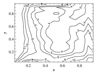
Figure 6: Reduced chi-square (total chi-square divided by the number of data points) contours from the SED fitting of YSO1 and YSO2 to determine the relative fraction factors of the WISE 22 µm flux ($x$) and the PACS 70 µm flux ($y$). $x$ and $y$ are the fraction factors of YSO1, i.e., the fraction factors of YSO2 are $(1-x)$ and $(1-y)$.

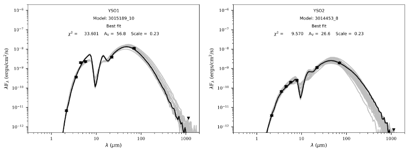
Figure 7: SEDs of YSO1 and YSO2 with the fitted SED models. Black lines present the best fitted model, and gray lines are the models satisfying the criterion of the goodness-of-fit, $\chi^{2}-\chi^{2}_{\rm best}<3\times n_{\rm data}$. Scale of 0.23 is the distance of 1.7 kpc in log scale.

The SED fitting results are shown in Figure 7. The black lines present the best-fitting models, and the gray lines present “good” models satisfying the criterion of $\chi^{2}-\chi^{2}_{\rm best}<3\times n_{\rm data}$, where $\chi^{2}$ is total chi-square from fitting, $\chi^{2}_{\rm best}$ is the total chi-square of the best-fitting model, and $n_{\rm data}$ is the number of data points used in fitting. The fitted parameters of the best models and the parameter ranges of good models are listed in Table 5. The evolutionary stages in the table have been determined by the Stage classification scheme of Robitaille et al. (2006), a scheme that is defined from the ratio of envelope accretion rate ($\dot{M}_{\rm env}$) or disk mass ($M_{\rm disk}$) to central source mass ($M_{\star}$): Stage I (including Stage 0) for the ones with $\dot{M}_{\rm env}/M_{\star}>10^{-6}~{}{\rm yr^{-1}}$; Stage II for the ones with $\dot{M}_{\rm env}/M_{\star}<10^{-6}~{}{\rm yr^{-1}}$ and $M_{\rm disk}/M_{\star}>10^{-6}$; and Stage III for the ones with $\dot{M}_{\rm env}/M_{\star}<10^{-6}~{}{\rm yr^{-1}}$ and $M_{\rm disk}/M_{\star}<10^{-6}$. The criterion of $\chi^{2}-\chi^{2}_{\rm best}<3\times n_{\rm data}$, we used to select good models, is the same as the one defined in Robitaille et al. (2007). Although this criterion is arbitrary and fairly loose in statistical aspects, as Robitaille et al. (2007) pointed out, it provides a range of acceptable fits to the eye and reasonable constraints. Considering the sparse coverage of 14-dimensional parameter space, the uncertainties of the models, and other realistic factors such as intrinsic variability or asymmetrical geometry of YSOs, this criterion also would prevent the risk of overinterpretation of SEDs from using a stricter criterion (Robitaille et al., 2007; Forbrich et al., 2010).

Table 5: SED Fitting Parameters of YSO1 and YSO2 from Good Models selected by $\chi^{2}-\chi^{2}_{\rm best}<3\times n_{\rm data}$

	YSO1				YSO2
Parameters	min	best	max		min	best	max
Central source mass ($M_{\sun}$)	7.94	9.96	10.1		5.27	5.39	7.64
Central source age (yr)	$1.18\times 10^{3}$	$3.21\times 10^{3}$	$2.53\times 10^{5}$		$2.62\times 10^{3}$	$2.62\times 10^{3}$	$9.79\times 10^{5}$
Total luminosity ($L_{\sun}$)	$1.87\times 10^{3}$	$2.20\times 10^{3}$	$4.42\times 10^{3}$		$2.87\times 10^{2}$	$4.60\times 10^{2}$	$1.46\times 10^{3}$
Central source temperature (K)	$4.13\times 10^{3}$	$4.32\times 10^{3}$	$2.46\times 10^{4}$		$4.17\times 10^{3}$	$4.17\times 10^{3}$	$2.01\times 10^{4}$
Envelope accretion rate ($M_{\sun}~{}{\rm yr^{-1}}$)	$2.88\times 10^{-5}$	$1.90\times 10^{-4}$	$2.63\times 10^{-4}$		$6.29\times 10^{-8}$	$6.77\times 10^{-5}$	$1.69\times 10^{-4}$
Disk mass ($M_{\sun}$)	0	0	$5.68\times 10^{-2}$		$9.03\times 10^{-5}$	$1.05\times 10^{-2}$	$4.78\times 10^{-1}$
Interstellar extinction, $A_{\rm V}$ (mag)	40.42	56.81	60.96		15.67	26.59	54.58
Stage		I				I/II

By the criterion of $\chi^{2}-\chi^{2}_{\rm best}<3\times n_{\rm data}$, 17 and 37 good models have been selected for YSO1 and YSO2, respectively, and all of the good models fairly well explain the observed SEDs of the two YSOs as seen in Figure 7, with the reduced chi-squares of 4.8–7.1 (YSO1) and 1.2–4.1 (YSO2). The parameter ranges presented in Table 5 are mostly within one or two order of magnitude except the envelope accretion rate and disk mass of YSO2, giving an ambiguous evolutionary stage between Stage I and II. These large parameter ranges can be improved if we have more data points, particularly far-IR/submillimeter data. Fluxes at longer wavebands significantly affect the determination of envelope accretion rate and disk mass as pointed out in Robitaille et al. (2007). We also tried fitting with distance varying in a range between 1.5 and 2 kpc. The increased number of free parameters increased the number of good models to 40 for YSO1 and 81 for YSO2, but their parameter ranges agree well with the ranges in Table 5, confirming that the uncertainty of distance insignificantly affects the fitting results. The mean distances derived from the fitting are 1.65 kpc and 1.71 kpc for YSO1 and YSO2, respectively, so the distance of 1.7 kpc we assumed is reasonable.

As indicated in Table 5, the young age and high envelope accretion rate of YSO1 confirm that it is a high-mass protostar, as previously implied by the detection of 6.7 GHz class II methanol maser (Pandian et al., 2011); YSO2, on the other hand, is rather close to an intermediate-mass YSO with lower mass. The evolutionary stage of Stage I, consistent with the class determined from the spectral index, indicates that either YSO1 or YSO2 can drive the outflow. Some models of YSO2 fall in Stage II with lower envelope accretion rate, but 80% of the models correspond to Stage I.

We note a large difference of interstellar extinction ($A_{\rm V}$) between YSO1 and YSO2. As this parameter $A_{\rm V}$ only accounts for external foreground extinction excluding the self-extinction by circumstellar dust, the two YSOs at the same distance are generally expected to have similar $A_{\rm V}$. But in Table 5, $A_{\rm V}$ of YSO1 is about two times larger than $A_{\rm V}$ of YSO2, although the maximum $A_{\rm V}$ is comparable. This is likely because YSO1 is almost at the center of the core where the extinction value is the maximum and YSO2 is a little away from the center where the extinction value is expected to be smaller. For example, the radial profiles of the mass surface density of IRDC cores at the distance of 2–3 kpc derived by mid-IR extinction technique (Butler & Tan, 2012) show that the mass surface densities are the maximum at $r<1\arcsec$ and gradually decrease to $\sim$40–60% of the maximum values at $r\sim 10\arcsec$ (Figures 5–12 of Butler & Tan, 2012). If G53.11_MM1 has a similar mass surface density profile to those IRDC cores, the mass surface density would decrease by a half at the position of YSO2 separated by $\sim$8$\arcsec$, and therefore, the difference of $A_{\rm V}$ between YSO1 and YSO2 from the SED fitting is acceptable. Additionally, we compare the extinction of YSO1 and YSO2 derived by their near-IR color. The $A_{\rm V}$ obtained by applying the H- and K-band magnitudes in Table 2 to the Equation 1 of Cooper et al. (2013) is $\sim$100 and $\sim$60 mag for YSO1 and YSO2, respectively. Since extinction from near-IR color includes dust-excess from circumstellar material (self-extinction), the derived $A_{\rm V}$ of the two YSOs are larger than $A_{\rm V}$ from the SED fitting or $N(^{13}{\rm CO})$, but they show a difference by about a factor of two, consistent with the $A_{\rm V}$ difference found in the SED fitting results.

6 Origin of the G53.11_MM1 Outflow

The G53.11_MM1 outflow is likely associated with the YSOs at the outflow center. Physical properties of the central YSOs examined in the previous section indicate that the both are capable of ejecting outflows, but which one is indeed driving the outflow is unclear. As described in Section 3.1.2, the overall morphology of the G53.11_MM1 outflow is bipolar with one lobe much brighter than the other. This bipolar morphology is in general interpreted as the outflow ejected from a single source with the brighter lobe blueshifted and the fainter lobe redshifted. If the whole outflow emission only originates from a single source, YSO2 seems to better explain the outflow morphology than YSO1. In Figure 8, we present vectors tracing the H₂ features on the H₂ emission contours at the top panel and on the continuum-subtracted Subaru/IRCS images at the bottom panels that show a detailed structure of the flows #1 and #2a. As drawn by the vectors from v1 to v12 in red color, YSO2 fairly well explains all of the emission features except #4 as the outflow with PA $\sim 74\arcdeg$ and opening angle $\sim 30\arcdeg$. The red vectors present at least three and five flows with different directions to the northeast and to the southwest, respectively. In particular, the flow #1 is clumpy and consists of several bow-shock flows as seen in the bottom right panel of Figure 8. Similar structures of multiple bow shocks have been observed in the high-resolution optical and near-IR images of HH1/HH2 and explained by thermal instabilities from the shock front running into inhomogeneous and perhaps rather dense ambient gas or by variability in jet direction (Hester et al., 1998; Davis et al., 2000). These radially propagating flows with bow-shock tips in the flow #1 are in part similar to the “H₂ fingers” of the Orion BN/KL outflow (Bally et al., 2015) produced by an explosive outflow with simultaneously ejected multiple jets from a high-mass YSO; however, when we consider the high degree of collimation and the small opening angle compared to the BN/KL outflow, a more feasible interpretation is multiple precessing jets. For example, if the outflow ejected from YSO2 experienced precession, the observed outflow morphology can be explained by at least two precessing jets.

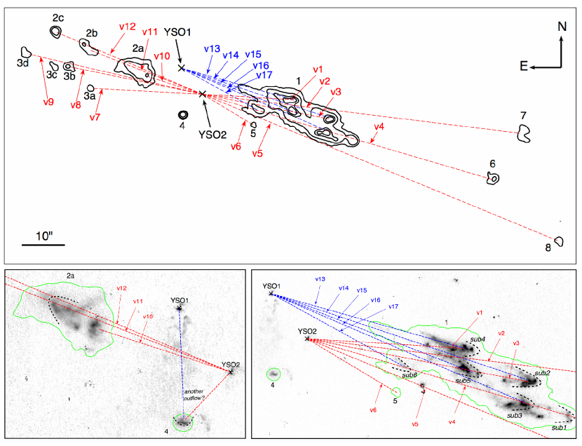
Figure 8: Top: H₂ outflow contours ($3\sigma,10\sigma,45\sigma$, and $80\sigma$ above the background in Figure 2) and the vectors that trace the outflow emission features by assuming the driving source as YSO1 (blue; from v13 to v17) and YSO2 (red; from v1 to v12). Bottom: Continuum-subtracted Subaru/IRCS H₂ images around the flow #1 and flow #2a with the outflow vectors. Possible bow-shock tips are drawn by black dashed-lines, and sub-flows in the flow #1 are labeled from sub1 to sub6.

Assuming YSO2 as a driving source, we can simply explain the entire outflow as discussed above, but it only describes the geometrical morphology that is projected on the sky, so we cannot rule out the possible contribution from YSO1 to the outflow. As the blue vectors from v13 to v17 in Figure 8 show, YSO1 well explains the H₂ emission features in the southwest. (The vectors tracing the features from #5 to #8 are not drawn for simplification.) In the bottom right panel of the figure, some sub-flows in the flow #1 are even better explained by YSO1, for example a faint bow-shock feature sub6 traced by v17, or a jet-like feature along v13. In this case, the outflow is defined by PA $\sim 67\arcdeg$ and opening angle $\sim 27\arcdeg$. Therefore, it can be suggested that the outflow toward southwest at least in part originates from YSO1 while its counter jet that is likely redshifted is not observed due to larger extinction to the opposite side. The H₂ emission in the northeast, on the other hand, are hardly traced by a vector from YSO1. If they originated from YSO1, a jet would have been ejected toward southeast and bent by $\sim$90$\arcdeg$ toward northeast. This requires the outflow to have experienced a high degree of precession, but it is not likely because curved or wiggly structures expected from precession are not seen among the other features. Another possible explanation for the NE flow in a relation with YSO1 is that the outflow axis has an inclination in the way that the NE axis is toward us, i.e., the NE lobe is blueshifted and the SW lobe is redshifted. This possibility conflicts with the general expectation that the blueshifted lobe is brighter than the redshifted one because of lower column density along the line of sight, but such expectation may not be applied if there is a region with locally enhanced extinction. The NE flow is closer to YSO1, i.e., the center of the core, than the SW flow, so the NE side is expected to have larger extinction than the SW side since extinction increases toward the center of the core as discussed in Section 5.2. Therefore, the NE flow can be a blueshifted lobe that is fainter than the other side due to locally larger extinction.

On the other hand, we can think of a possibility that there is another outflow-driving source in the core besides YSO1 and YSO2 that has not yet been detected. As a protostar can eject outflows from very young evolutionary phase surrounded by a thick envelope, outflow-driving YSOs are often so deeply embedded that they are not observed in near- or mid-IR but only observed in (sub)millimeter (e.g., LkH$\alpha$ 234 region; Fuente et al., 2001). In addition, recent ALMA observations have revealed that a massive core in fact is composed of several lower-mass cores embedded in a dust filament, cores that can be only resolved at high angular resolution of $\lesssim 1\arcsec$ (e.g., G35.20-0.74; Sánchez-Monge et al., 2014), suggesting that G53.11_MM1 also possibly contains undetected, deeply embedded protostars driving the H₂ outflow. We note that the outflow luminosity derived in Section 3.2 implies $\sim 10^{4}<L_{\rm bol}/L_{\sun}<10^{6}$ for the driving source on the relation of $L_{\rm H_{2}}\propto L_{\rm bol}^{0.6}$ (Caratti o Garatti et al., 2015). If this empirical relation works here, the luminosity of YSO1 ($\sim 2\times 10^{3}~{}L_{\sun}$) and YSO2 ($\sim 0.5\times 10^{3}~{}L_{\sun}$) inferred from SED fitting does not seem to be enough to explain the observed outflow luminosity. This may imply the possible presence of another outflow-driving source that may be massive enough to solely eject the observed H₂ outflow, but it is more feasible that the G53.11_MM1 outflow is composed of multiple outflows of different origins including YSO1 and YSO2, for they are all very young YSOs in early phase expected to eject outflows.

Lastly, we discuss about the H₂ emission feature #4. In the UKIRT image (Figure 2), #4 appears as a compact knot, but in the Subaru image (the bottom panels of Figure 8), it appears as a small, thin filament with a curvature similar to a bow-shock tip of which apex is well connected to either YSO1 or YSO2. As discussed in Section 3.1.4, the PA of #4 with respect to either YSO is very different from the PAs of the other emission features or the overall PA of the outflow, suggesting that there may be another outflow differentiated from the NW-SE outflow. There are also a small, elongated feature at the west of #4 at the level of one sigma above the background (Figure 2) and faint features between YSO1 and #4 (Figure 8) although the latter are not clear whether they are real H₂ emission or residual nebula emission left from continuum subtraction. If the faint elongated feature is also a part of another outflow with #4, the outflow direction is from north to south and the driving source is likely YSO1.

7 Summary and Conclusion

We have presented a parsec-scale H₂ outflow discovered in the IRDC core G53.11_MM1 at the distance of 1.7 kpc. The overall morphology of the outflow is bipolar along the NE-SW direction in the H₂ 1-0 S(1) 2.12 µm image. At the outflow center, there are two Class I YSOs (YSO1 and YSO2) separated by $\sim$8$\arcsec$; we consider both to be putative outflow-driving sources based on their IR colors and location. We derived the physical parameters of the H₂ outflow and the central YSOs using the H₂ images and the broad-band near-IR images, and have discussed their association. Our results and the implications on the properties and origin of the outflow can be summarized as follows.

1. The outflow is bipolar from northeast to southwest with the SW flow is much brighter than the NE flow, but the detailed structure is composed of several discrete flows and knots. From the UKIRT H₂ image, we identified 13 emission features using the threshold of three sigma above the background. The outflow, with the total length of $\sim$130$\arcsec$ or $\sim$1 pc at 1.7 kpc, is relatively long compared with the observed protostellar outflows from low-mass YSOs. The dynamical age, although it highly depends on outflow velocity, is from several thousand to a few tens of thousand years. Some of the H₂ emission features are well aligned and show time gaps about 1,000 yr at the outflow velocity of 80 km s^-1; a few thousand years of time gaps are comparable to the time gaps reported in previous studies (e.g, Ioannidis & Froebrich, 2012b; Froebrich & Makin, 2016) and suggest episodic or non-steady mass ejection history. The position angle of the outflow is uncertain without a confirmed driving source but is around 70$\arcdeg$.

2. The total extinction-corrected H₂ luminosity of the outflow is $L_{\rm H_{2}}\sim$ (6–150) $L_{\sun}$. We adopt an Av of between 15 and 50 mag, based on the average optical depth of a larger scale Spitzer dark cloud including G53.11_MM1 and ¹³CO column density, respectively. If the whole outflow is ejected from a single source, the observed H₂ luminosity that is several times larger than the luminosity of the outflows from low-/intermediate-mass YSOs (Caratti o Garatti et al., 2006; Ioannidis & Froebrich, 2012b) implies a high-mass outflow-driving source for the G53.11_MM1 outflow. The empirical relationship between the H₂ luminosity of the outflow and the bolometric luminosity of the driving source ($L_{\rm H_{2}}\propto L_{\rm bol}^{\alpha}$ with $\alpha\sim 0.6$; Caratti o Garatti et al., 2015) also suggests that the driving source of the G53.11_MM1 outflow is massive with $\sim 10^{4}<L_{\rm bol}/L_{\sun}<10^{6}$.

3. We identified compact, faint [Fe II] emission features from the high-resolution Subaru/IRCS image. The [Fe II] emission is marginally detected inside the H₂ flows with the area of $\sim$1 arcsec² and the surface brightness about ten times smaller than the H₂ brightness. But it is difficult to conclude that the detected [Fe II] emission is associated with the H₂ outflow because [Fe II] knots are generally observed at the tips of the H₂ jets rather than behind the H₂ bow shocks. Since the H₂ and [Fe II] lines arise from different shock origins, the marginal detection of [Fe II] emission may indicate that slow, C-type shocks are dominant in the G53.11_MM1 outflow, although deeper imaging observations with higher sensitivity or spectroscopic observations are required to derive the physical conditions of the region and confirm shock properties.

4. Both central YSOs show photometric variability in H- and K-bands between several years. The available data are limited to present the full variability, but high variability amplitudes of $\gtrsim$1 mag suggest that they can be eruptive variable YSOs with episodic outbursts. The SED fitting of the two YSOs shows that both YSOs are indeed in the early evolutionary stage with high envelope accretion rates of $10^{-5}$–$10^{-4}M_{\sun}~{}{\rm yr}^{-1}$, implying that the both are proper candidates of the outflow-driving source. The masses inferred from the best SED fitting models are $\sim$10 $M_{\sun}$ and $\sim$5 $M_{\sun}$ for YSO1 and YSO2, respectively. This supports the association between the H₂ outflow and a high-mass YSO, and also confirms high-mass star formation occurring in the IRDC core.

5. The G53.11_MM1 outflow is most likely associated with the two central YSOs. The young evolutionary stages of both YSOs support their association, but which one is driving the outflow is still unclear. YSO2 well explains the geometrical morphology of the outflow as a single-source origin. But we cannot rule out the possible contribution from YSO1 because it also well describes the outflow emission in the southwest, and may explains the emission in the northeast as well if the NE axis of the outflow is toward us. The outflow, by assuming either YSO as a driving source, can be defined by PA $\sim 70\arcdeg$ and opening angle $\sim 30\arcdeg$; the radial flows of different directions with bow-shock tips may suggest multiple precessing jets. In addition, we consider a possibility of the presence of another outflow-driving source very deeply embedded in the core that has not been detected in near- and mid-IR but could be detected in the submillimiter with high-spatial resolution.

6. Our results show that the G53.11_MM1 outflow has a complicated morphology with more than one outflow-driving source candidates. One of the H₂ features with very different PA from the other features even raises a possibility that there is another outflow, implying that the G53.11_MM1 outflow is a combination of multiple outflows of several different origins. Our study also implies that the parsec-scale, collimated H₂ outflow, at least in part, originates from a massive ($\sim$10 $M_{\sun}$) YSO as well as an intermediate-mass ($\gtrsim$5 $M_{\sun}$) YSO, suggesting intermediate- to high-mass star formation by mass accretion via disks as low-mass star formation. Follow-up observations particularly to obtain the kinematic information of the outflow and to search for molecular outflows directly ejected from the central YSOs will be necessary in order to confirm these possibilities and fully understand the outflow characteristics in future.

References

- Aguirre et al. (2011) Aguirre, J. E., Ginsburg, A. G., Dunham, M. K., et al. 2011, ApJS, 192, 4
- Alves de Oliveira & Casali (2008) Alves de Oliveira, C., & Casali, M. 2008, A&A, 485, 155
- Bally et al. (2015) Bally, J., Ginsburg, A., Silvia, D., & Youngblood, A. 2015, A&A, 579, A130
- Benjamin et al. (2003) Benjamin, R. A., Churchwell, E., Babler, B. L., et al. 2003, PASP, 115, 953
- Beuther et al. (2002) Beuther, H., Schilke, P., Gueth, F., et al. 2002, A&A, 387, 931
- Bonnell et al. (2001) Bonnell, I. A., Bate, M. R., Clarke, C. J., & Pringle, J. E. 2001, MNRAS, 323, 785
- Butler & Tan (2012) Butler, M. J., & Tan, J. C. 2012, ApJ, 754, 5
- Chapman et al. (2009) Chapman, N. L., Mundy, L. G., Lai, S.-P., & Evans, N. J., II 2009, ApJ, 690, 496
- Caratti o Garatti et al. (2006) Caratti o Garatti, A., Giannini, T., Nisini, B., & Lorenzetti, D. 2006, A&A, 449, 1077
- Caratti o Garatti et al. (2015) Caratti o Garatti, A., Stecklum, B., Linz, H., Garcia Lopez, R., & Sanna, A. 2015, A&A, 573, A82
- Carey et al. (2009) Carey, S. J., Noriega-Crespo, A., Mizuno, D. R., et al. 2009, PASP, 121, 76
- Carpenter et al. (2001) Carpenter, J. M., Hillenbrand, L. A., & Skrutskie, M. F. 2001, AJ, 121, 3160
- Carpenter et al. (2002) Carpenter, J. M., Hillenbrand, L. A., Skrutskie, M. F., & Meyer, M. R. 2002, AJ, 124, 1001
- Christou et al. (2010) Christou, J. C., Neichel, B., Rigaut, F., et al. 2010, Proc. SPIE, 7736, 77361R
- Churchwell et al. (2009) Churchwell, E., Babler, B. L., Meade, M. R., et al. 2009, PASP, 121, 213
- Contreras Peña et al. (2017a) Contreras Peña, C., Lucas, P. W., Kurtev, R., et al. 2017a, MNRAS, 465, 3039
- Contreras Peña et al. (2017b) Contreras Peña, C., Lucas, P. W., Minniti, D., et al. 2017b, MNRAS, 465, 3011
- Cooper et al. (2013) Cooper, H. D. B., Lumsden, S. L., Oudmaijer, R. D., et al. 2013, MNRAS, 430, 1125
- Davis et al. (2009) Davis, C. J., Froebrich, D., Stanke, T., et al. 2009, A&A, 496, 153
- Davis et al. (2010) Davis, C. J., Gell, R., Khanzadyan, T., Smith, M. D., & Jenness, T. 2010, A&A, 511, A24
- Davis et al. (2008) Davis, C. J., Scholz, P., Lucas, P., Smith, M. D., & Adamson, A. 2008, MNRAS, 387, 954
- Davis et al. (2000) Davis, C. J., Smith, M. D., & Eislöffel, J. 2000, MNRAS, 318, 747
- Davis et al. (1999) Davis, C. J., Smith, M. D., Eislöffel, J., & Davies, J. K. 1999, MNRAS, 308, 539
- Davis et al. (2004) Davis, C. J., Varricatt, W. P., Todd, S. P., & Ramsay Howat, S. K. 2004, A&A, 425, 981
- Diolaiti et al. (2000) Diolaiti, E., Bendinelli, O., Bonaccini, D., et al. 2000, Proc. SPIE, 4007, 879
- Dunham et al. (2014) Dunham, M. M., Stutz, A. M., Allen, L. E., et al. 2014, Protostars and Planets VI, 195
- Dye et al. (2006) Dye, S., Warren, S. J., Hambly, N. C., et al. 2006, MNRAS, 372, 1227
- Flaherty et al. (2007) Flaherty, K. M., Pipher, J. L., Megeath, S. T., et al. 2007, ApJ, 663, 1069
- Forbrich et al. (2010) Forbrich, J., Tappe, A., Robitaille, T., et al. 2010, ApJ, 716, 1453
- Frank et al. (2014) Frank, A., Ray, T. P., Cabrit, S., et al. 2014, Protostars and Planets VI, 451
- Froebrich et al. (2011) Froebrich, D., Davis, C. J., Ioannidis, G., et al. 2011, MNRAS, 413, 480
- Froebrich & Makin (2016) Froebrich, D., & Makin, S. V. 2016, MNRAS, 462, 1444
- Froebrich et al. (2015) Froebrich, D., Makin, S. V., Davis, C. J., et al. 2015, MNRAS, 454, 2586
- Fuente et al. (2001) Fuente, A., Neri, R., Martín-Pintado, J., et al. 2001, A&A, 366, 873
- Giannini et al. (2004) Giannini, T., McCoey, C., Caratti o Garatti, A., et al. 2004, A&A, 419, 999
- Greene et al. (1994) Greene, T. P., Wilking, B. A., Andre, P., Young, E. T., & Lada, C. J. 1994, ApJ, 434, 614
- Gutermuth et al. (2009) Gutermuth, R. A., Megeath, S. T., Myers, P. C., et al. 2009, ApJS, 184, 18
- Hayano et al. (2010) Hayano, Y., Takami, H., Oya, S., et al. 2010, Proc. SPIE, 7736, 77360N
- Hayashi & Pyo (2009) Hayashi, M., & Pyo, T.-S. 2009, ApJ, 694, 582
- Hester et al. (1998) Hester, J. J., Stapelfeldt, K. R., & Scowen, P. A. 1998, AJ, 116, 372
- Hodapp et al. (2003) Hodapp, K. W., Jensen, J. B., Irwin, E. M., et al. 2003, PASP, 115, 1388
- Hodgkin et al. (2009) Hodgkin, S. T., Irwin, M. J., Hewett, P. C., & Warren, S. J. 2009, MNRAS, 394, 675
- Indebetouw et al. (2005) Indebetouw, R., Mathis, J. S., Babler, B. L., et al. 2005, ApJ, 619, 931
- Ioannidis & Froebrich (2012a) Ioannidis, G., & Froebrich, D. 2012a, MNRAS, 421, 3257
- Ioannidis & Froebrich (2012b) Ioannidis, G., & Froebrich, D. 2012b, MNRAS, 425, 1380
- Jackson et al. (2006) Jackson, J. M., Rathborne, J. M., Shah, R. Y., et al. 2006, ApJS, 163, 145
- Johnstone et al. (2013) Johnstone, D., Hendricks, B., Herczeg, G. J., & Bruderer, S. 2013, ApJ, 765, 133
- Kang et al. (2015) Kang, H., Kim, K.-T., Byun, D.-Y., Lee, S., & Park, Y.-S. 2015, ApJS, 221, 6
- Khanzadyan et al. (2003) Khanzadyan, T., Smith, M. D., Davis, C. J., et al. 2003, MNRAS, 338, 57
- Kim et al. (2015) Kim, H.-J., Koo, B.-C., & Davis, C. J. 2015, ApJ, 802, 59
- Kim et al. (1994) Kim, S.-H., Martin, P. G., & Hendry, P. D. 1994, ApJ, 422, 164
- Kobayashi et al. (2000) Kobayashi, N., Tokunaga, A. T., Terada, H., et al. 2000, Proc. SPIE, 4008, 1056
- Lada (1987) Lada, C. J. 1987, Star Forming Regions, 115, 1
- Lee et al. (2013) Lee, H.-T., Liao, W.-T., Froebrich, D., et al. 2013, ApJS, 208, 23
- Lee et al. (2014) Lee, J.-J., Koo, B.-C., Lee, Y.-H., et al. 2014, MNRAS, 443, 2650
- López et al. (2010) López, R., Acosta-Pulido, J. A., Gómez, G.,Estalella, R., & Carrasco-González, C. 2010, A&A, 523, A16
- López-Sepulcre et al. (2009) López-Sepulcre, A., Codella, C., Cesaroni, R., Marcelino, N., & Walmsley, C. M. 2009, A&A, 499, 811
- Lucas et al. (2008) Lucas, P. W., Hoare, M. G., Longmore, A., et al. 2008, MNRAS, 391, 136
- Lumsden et al. (2013) Lumsden, S. L., Hoare, M. G., Urquhart, J. S., et al. 2013, ApJS, 208, 11
- McKee & Tan (2003) McKee, C. F., & Tan, J. C. 2003, ApJ, 585, 850
- Milam et al. (2005) Milam, S. N., Savage, C., Brewster, M. A., Ziurys, L. M., & Wyckoff, S. 2005, ApJ, 634, 1126
- Molinari et al. (2010) Molinari, S., Swinyard, B., Bally, J., et al. 2010, PASP, 122, 314
- Morales-Calderón et al. (2011) Morales-Calderón, M., Stauffer, J. R., Hillenbrand, L. A., et al. 2011, ApJ, 733, 50
- Mottram et al. (2011) Mottram, J. C., Hoare, M. G., Urquhart, J. S., et al. 2011, A&A, 525, A149
- Nisini et al. (2002) Nisini, B., Caratti o Garatti, A., Giannini, T., & Lorenzetti, D. 2002, A&A, 393, 1035
- Pandian et al. (2011) Pandian, J. D., Momjian, E., Xu, Y., Menten, K. M., & Goldsmith, P. F. 2011, ApJ, 730, 55
- Peretto & Fuller (2009) Peretto, N., & Fuller, G. A. 2009, A&A, 505, 405
- Pineda et al. (2010) Pineda, J. L., Goldsmith, P. F., Chapman, N., et al. 2010, ApJ, 721, 686
- Raga et al. (2013) Raga, A. C., Noriega-Crespo, A., Carey, S. J., & Arce, H. G. 2013, AJ, 145, 28
- Ragan et al. (2014) Ragan, S. E., Henning, T., Tackenberg, J., et al. 2014, A&A, 568, AA73
- Rathborne et al. (2006) Rathborne, J. M., Jackson, J. M., & Simon, R. 2006, ApJ, 641, 389
- Rebull et al. (2015) Rebull, L. M., Stauffer, J. R., Cody, A. M., et al. 2015, AJ, 150, 175
- Reipurth et al. (2000) Reipurth, B., Yu, K. C., Heathcote, S., Bally, J., & Rodríguez, L. F. 2000, AJ, 120, 1449
- Robitaille et al. (2007) Robitaille, T. P., Whitney, B. A., Indebetouw, R., & Wood, K. 2007, ApJS, 169, 328
- Robitaille et al. (2006) Robitaille, T. P., Whitney, B. A., Indebetouw, R., Wood, K., & Denzmore, P. 2006, ApJS, 167, 256
- Sánchez-Monge et al. (2014) Sánchez-Monge, Á., Beltrán, M. T., Cesaroni, R., et al. 2014, A&A, 569, A11
- Shu et al. (1994) Shu, F., Najita, J., Ostriker, E., et al. 1994, ApJ, 429, 781
- Simon et al. (2006) Simon, R., Jackson, J. M., Rathborne, J. M., & Chambers, E. T. 2006, ApJ, 639, 227
- Skrutskie et al. (2006) Skrutskie, M. F., Cutri, R. M., Stiening, R., et al. 2006, AJ, 131, 1163
- Smith et al. (1997) Smith, M. D., Davis, C. J., & Lioure, A. 1997, A&A, 327, 1206
- Stanke et al. (2002) Stanke, T., McCaughrean, M. J., & Zinnecker, H. 2002, A&A, 392, 239
- Tan et al. (2014) Tan, J. C., Beltrán, M. T., Caselli, P., et al. 2014, Protostars and Planets VI, 149
- Tody (1986) Tody, D. 1986, Proc. SPIE, 627, 733
- Tody (1993) Tody, D. 1993, Astronomical Data Analysis Software and Systems II, 52, 173
- Tokunaga et al. (1998) Tokunaga, A. T., Kobayashi, N., Bell, J., et al. 1998, Proc. SPIE, 3354, 512
- Traficante et al. (2015) Traficante, A., Fuller, G. A., Peretto, N., Pineda, J. E., & Molinari, S. 2015, MNRAS, 451, 3089
- Urquhart et al. (2009) Urquhart, J. S., Hoare, M. G., Purcell, C. R., et al. 2009, A&A, 501, 539
- Varricatt et al. (2010) Varricatt, W. P., Davis, C. J., Ramsay, S., & Todd, S. P. 2010, MNRAS, 404, 661
- Wang et al. (2010) Wang, P., Li, Z.-Y., Abel, T., & Nakamura, F. 2010, ApJ, 709, 27
- Wenger et al. (2000) Wenger, M., Ochsenbein, F., Egret, D., et al. 2000, A&AS, 143, 9
- Whitney et al. (2003a) Whitney, B. A., Wood, K., Bjorkman, J. E., & Cohen, M. 2003a, ApJ, 598, 1079
- Whitney et al. (2003b) Whitney, B. A., Wood, K., Bjorkman, J. E., & Wolff, M. J. 2003b, ApJ, 591, 1049
- Wolf-Chase et al. (2013) Wolf-Chase, G., Arvidsson, K., Smutko, M., & Sherman, R. 2013, ApJ, 762, 87
- Wolk et al. (2013) Wolk, S. J., Rice, T. S., & Aspin, C. 2013, ApJ, 773, 145
- Wright et al. (2010) Wright, E. L., Eisenhardt, P. R. M., Mainzer, A. K., et al. 2010, AJ, 140, 1868
- Wu et al. (2005) Wu, Y., Zhang, Q., Chen, H., et al. 2005, AJ, 129, 330