THE STAR FORMATION EFFICIENCY PER FREE FALL TIME IN NEARBY GALAXIES

Abstract

We estimate the star formation efficiency per gravitational free fall time, $\epsilon_{\rm ff}$, from observations of nearby galaxies with resolution matched to the typical size of a Giant Molecular Cloud. This quantity, $\epsilon_{\rm ff}$, is theoretically important but so far has only been measured for Milky Way clouds or inferred indirectly in a few other galaxies. Using new, high resolution CO imaging from the PHANGS-ALMA survey, we estimate the gravitational free-fall time at 60 to 120 pc resolution, and contrast this with the local molecular gas depletion time to estimate $\epsilon_{\rm ff}$. Assuming a constant thickness of the molecular gas layer ($H=100$ pc) across the whole sample, the median value of $\epsilon_{\rm ff}$ in our sample is $0.7\%$. We find a mild scale-dependence, with higher $\epsilon_{\rm ff}$ measured at coarser resolution. Individual galaxies show different values of $\epsilon_{\rm ff}$, with the median $\epsilon_{\rm ff}$ ranging from $0.3\%$ to $2.6\%$. We find the highest $\epsilon_{\rm ff}$ in our lowest mass targets, reflecting both long free-fall times and short depletion times, though we caution that both measurements are subject to biases in low mass galaxies. We estimate the key systematic uncertainties, and show the dominant uncertainty to be the estimated line-of-sight depth through the molecular gas layer and the choice of star formation tracers.

1 Introduction

Star formation is “inefficient,” meaning that the star formation rate is low compared to what would be expected if cold gas collapsed directly into stars (see review by McKee & Ostriker, 2007; Krumholz, 2014). Theoretical models of star formation in molecular clouds that attempt to explain this inefficiency include turbulent support (Krumholz & McKee, 2005; Padoan et al., 2012), destructive feedback (Murray et al., 2010), magnetic fields (Federrath, 2015), and dynamical stabilization (Ostriker et al., 2010; Meidt et al., 2018).

Over the last decade, many of these models have expressed their predictions in terms of the efficiency of star formation per free fall time, $\epsilon_{\rm ff}$. This $\epsilon_{\rm ff}$ is the fraction of gas converted into stars per gravitational free fall time, $\tau_{\rm ff}$. As such, $\epsilon_{\rm ff}$ expresses the inefficiency of star formation relative to free-fall collapse. Theoretical predictions for $\epsilon_{\rm ff}$ on cloud scales span the range from $\sim 0.1\%$ to few times $10\%$ (McKee & Ostriker, 2007; Krumholz et al., 2012; Federrath & Klessen, 2012; Padoan et al., 2012; Raskutti et al., 2016), with higher values possible for clouds with active star formation (Murray, 2011; Lee et al., 2016) or the densest parts of clouds (Evans et al., 2014). From numerical simulations, $\epsilon_{\rm ff}$ increases strongly from low values in unbound gas to high values when the virial parameter is near unity (Padoan et al., 2012).

In spite of the fact that $\epsilon_{\rm ff}$ is the central prediction of many current models of star formation, observational constraints on this quantity have remained challenging. The issue is that $\tau_{\rm ff}$ depends on the volume density of the gas, $\rho$, via

$$\mbox{$\tau_{\rm ff}$}=\sqrt{\frac{3\pi}{32G\rho}}~{},$$ (1)

and it is difficult to directly measure $\rho$ at cloud scales. This requires either high resolution imaging or density-sensitive multi-line spectroscopy (Gao & Solomon, 2004a; Leroy et al., 2017b).

Indirect estimates of $\epsilon_{\rm ff}$ are common. For example, Murray (2011), Evans et al. (2014), Lee et al. (2016), and Vutisalchavakul et al. (2016) estimated $\epsilon_{\rm ff}$ $\approx 0.4-1.6\%$ for populations of star-forming clouds in the Milky Way (MW), and Barnes et al. (2017) obtained $\epsilon_{\rm ff}$ $\approx 1-4\%$ in the central few hundred parsec of the MW. Ochsendorf et al. (2017) extended such studies to the Large Magellanic Cloud, where they found $\epsilon_{\rm ff}$ in the range of $12-25\%$ (depending on the adopted SFR tracer) and showed that $\epsilon_{\rm ff}$ decreases with increasing cloud mass. The above findings for $\epsilon_{\rm ff}$ are mean values; all of the above studies of individual GMCs (as well as earlier work by Mooney & Solomon, 1988) showed a large range of efficiency, much of which maybe due to cloud’s evolution. Leroy et al. (2017a) estimated $\epsilon_{\rm ff}$ $\approx 0.30-0.36\%$ in M51, based on the PAWS survey (Schinnerer et al., 2013), and Schruba et al. (2018b) found $\epsilon_{\rm ff}$ $\approx 0.1-1\%$ in the MW and 7 nearby galaxies. However, we still lack a statistically significant sample of $\epsilon_{\rm ff}$ across the local galaxy population.

The most general measurement to date comes from observations of dense gas, as traced by high critical density line emission (e.g., HCN; Gao & Solomon, 2004b). By equating the mean gas density of an emission line with its critical density, and adopting a dense gas conversion factor, they can infer $\epsilon_{\rm ff}$. This approach has been taken by Krumholz & Tan (2007) and García-Burillo et al. (2012), who concluded that $\epsilon_{\rm ff}$ is approximately constant ($0.5-1\%$). Subsequently, numerous other studies (Longmore et al., 2013; Kruijssen et al., 2014; Usero et al., 2015; Bigiel et al., 2016; Gallagher et al., 2018) have used similar techniques to find an environmentally-dependent $\epsilon_{\rm ff}$ ($0.2-4\%$).

The PHANGS collaboration is now using ALMA to map the molecular gas in 74 nearby galaxies with resolution matched to the scale of an individual Giant Molecular Cloud. These observations recover the surface density of molecular gas at high physical resolution, which is closely related to the mean volume density. In this Letter, we combine the first $11$ CO(2–1) maps from PHANGS-ALMA with three CO maps from the literature. From these maps, we infer $\tau_{\rm ff}$ and compare it to the measured gas depletion time to estimate $\epsilon_{\rm ff}$. This yields the largest and most direct sample of extragalactic $\epsilon_{\rm ff}$ measurements to date. After describing our data in $\S$2 and explaining our methodology in $\S$3, we present the key results in $\S$4 and summarize them in $\S$5.

2 Data

2.1 Molecular Gas

We estimate molecular gas surface density from PHANGS-ALMA CO (2–1) data for $11$ targets and archival CO data for M31 (A. Schruba et al. in preparation; Caldú-Primo & Schruba, 2016), M33 (Druard et al., 2014), and M51 (Schinnerer et al., 2013). PHANGS-ALMA uses ALMA’s 12m, 7m, and total power antennas to map CO (2–1) emission from nearby ($d\lesssim 17$ Mpc) galaxies at native angular resolution of $1-1.5\arcsec$. This translates to native physical resolutions of $\sim~{}60{-}120$ pc depending on the distance to the target. At their native resolutions, the CO data cubes have rms noise of $\sim 0.1$ K per $2.5$ km s^-1 channel. The inclusion of the ACA 7m and total power data means that we expect these maps to be sensitive to emission at all spatial scales.

The sample selection, observing strategy, reduction, and properties of the full $74$ galaxies in PHANGS-ALMA survey is presented in A. K. Leroy et al. (in preparation). Here, we use the first data sets, including three literature maps, where the CO surface brightness and line-width have been calculated by Sun et al. (2018). See that paper for a detailed presentation of masking, map construction, and completeness.

We adopt a fixed CO(2–1)-to-H₂ conversion factor $\alpha_{\rm CO}^{2-1}=6.2$ M_⊙ pc^-2 (K km s^-1)^-1. This combines the commonly adopted Galactic CO(1–0) conversion factor, $\alpha_{\rm CO}^{1-0}=4.35$ M_⊙ pc^-2 (K km s^-1)^-1 (Bolatto et al., 2013), including the contribution from Helium, with a typical CO(2–1)/CO(1–0) line ratio of 0.7 (e.g., Sakamoto et al., 1997; Leroy et al., 2013). Then, we convert the CO(2–1) integrated intensity, $I_{\rm CO}^{2-1}$, to $\Sigma_{\rm mol}$ via:

$$\Sigma_{\rm mol}{\rm\left[M_{\odot}~{}pc^{-2}\right]}=\alpha_{\rm CO}^{2-1}\ I_{\rm CO}^{2-1}~{}{\rm\left[K~{}km~{}s^{-1}\right]}~{},$$ (2)

The M31 and M51 CO maps target the CO(1–0) line. For those we use $\alpha_{\rm CO}^{1-0}=4.35$ M_⊙ pc^-2 (K km s^-1)^-1 with no line ratio term. We apply inclination corrections to all measured surface densities.

Our sample includes a few low mass (down to $4~{}\times~{}10^{9}~{}M_{\odot}$), low metallicity galaxies. We explore the effect of a metallicity-dependent $\alpha_{\rm CO}$ on our results for these cases. The fraction of ‘CO-dark‘ molecular gas increases with decreasing metallicity, resulting in higher $\alpha_{\rm CO}$ (Bolatto et al., 2013). We use metallicities compiled by Pilyugin et al. (2004, their Table 5), except for M33 and M51, where we adopt metallicities from Rosolowsky & Simon (2008) and Croxall et al. (2015), respectively, and NGC 1672, NGC 3627, and NGC 4535, for which we adopt metallicities from K. Kreckel et al. in preparation based on new VLT-MUSE observations. All metallicites are quoted at $0.4~{}R_{25}$. We calculate the metallicity-dependent $\alpha_{\rm CO}$ following the prescription of Bolatto et al. (2013). Beyond metallicity effects, the central regions of many galaxies shows smaller $\alpha_{\rm CO}$ (Sandstrom et al., 2013). Our key result in this paper is weighted by area and the center covers only a few lines-of-sight, so we defer investigation of the impact of this effect to future papers.

2.2 Recent Star Formation

We derive the star formation rate (SFR) surface density, $\Sigma_{\rm SFR}$, from WISE infrared and GALEX UV maps (A. K. Leroy et al. in preparation). The WISE maps are derived from the unWISE reprocessing of Lang (2014). The GALEX maps are coadded, convolved, background subtracted maps constructed from the full-mission GALEX archive (Martin & GALEX Team, 2005). We correct the FUV and NUV maps for Galactic extinction using $E(B-V)$ from the map of Schlegel et al. (1998) converted to the GALEX bands using the $R_{\rm NUV}$ and $R_{\rm FUV}$ values from Peek & Schiminovich (2013). Both sets of maps are convolved to have matched Gaussian beams ($15^{\prime\prime}$ FWHM, which corresponds to $1.3$ kpc at our most distant target) and background-subtracted using control regions outside the galaxy.

We convert FUV, NUV, 12$\mu$m, and $22\mu$m intensity, $I_{\nu}$, to an estimate of the recent SFR using

$$\Sigma_{\rm SFR}\ [{\rm M_{\odot}~{}yr}^{-1}{\rm kpc}^{-2}]\approx K\ I_{\nu}\ [{\rm MJy\ sr}^{-1}],$$ (3)

where $K=1.04\times 10^{-1}$, $1.04\times 10^{-1}$, $3.77\times 10^{-3}$, and $2.97\times 10^{-3}$ for FUV, NUV, 12µm, and 24µm bands, respectively (Kennicutt & Evans, 2012; Jarrett et al., 2013). We use hybrid tracers by adding the SFR derived from each choice of UV and IR band, and adopt SFR(FUV+22µm) as a benchmark. To estimate systematic uncertainties, we test the effect of using NUV instead of FUV and using 12µm instead of 22µm.

3 Methodology

We estimate $\epsilon_{\rm ff}$ from the ratio between the gravitational free fall time of molecular gas, $\tau_{\rm ff}$, and the molecular gas depletion time, $\tau_{\rm dep}^{\rm mol}$.

3.1 Molecular Gas Depletion Time

We calculate $\tau_{\rm dep}^{\rm mol}$ at $1.3$ kpc resolution across each target as

$$\mbox{$\tau_{\rm dep,\,1.3kpc}^{\rm mol}$}=\frac{\mbox{$\Sigma_{\rm mol,1.3kpc}$}}{\mbox{$\Sigma_{\rm SFR,1.3kpc}$}}.$$ (4)

Here, $\Sigma_{\rm mol,1.3kpc}$ is the convolved $\Sigma_{\rm mol}$ at 1.3 kpc FWHM to match the resolution of $\Sigma_{\rm SFR,1.3kpc}$ maps. We treat this as our working resolution to estimate $\tau_{\rm dep}^{\rm mol}$.

3.2 Molecular Gas Free Fall Time

We estimate $\tau_{\rm ff}$ following Equation 1. This requires an estimate of the mass volume density, $\rho$. To estimate $\rho$, we combine our measured, high physical resolutions ($60{-}120$ pc) $\Sigma_{\rm mol}$ with an estimate of the line-of-sight depth through the molecular gas layer, $H$, so that:

$$\rho\approx\frac{\mbox{$\Sigma_{\rm mol}$}}{H}~{}.$$ (5)

We describe how we estimate $H$ in $\S$3.3. We combine Equations 1 and 5 to estimate $\tau_{\rm ff}$ as

$$\tau_{\rm ff,60pc}=\sqrt{\frac{3\pi}{32G}\left(\frac{H}{\mbox{$\Sigma_{\rm mol,60pc}$}}\right)}.$$ (6)

We make analogous measurements of $\tau_{\rm ff}$ at $80$, $100$, and $120$ pc resolution, as permitted by the native resolution of the data.

3.3 Thickness of the Molecular Gas Layer

To translate a measured molecular gas surface density into a volume density, we must estimate the line of sight depth of the molecular gas layer, $H$. We define $H$ so that $\rho=\mbox{$\Sigma_{\rm mol}$}/H$. We explore three approaches:

1. Fixed $H=100$ pc. This is roughly the diameter of a large molecular cloud and a characteristic thickness (FWHM) of the molecular gas layer in the Milky Way and other galaxies (Heyer & Dame, 2015; Yim et al., 2014; Pety et al., 2013). This is our default value.

2. In hydrostatic equilibrium, the turbulent midplane pressure of molecular gas balances the vertical weight of the molecular gas column in the potential of the disk. If we consider only gas responding to the potential well defined by stars, i.e., neglecting gas self-gravity, then

   $$H\,\equiv\,2h\approx\,\sqrt{\frac{\sigma_{\rm mol}^{2}~{}h_{*}}{G\,\Sigma_{*}}}~{},$$ (7)

   following Ostriker et al. (2010). Here $\sigma_{\rm mol}$ is the velocity dispersion of the molecular gas, $\Sigma_{*}$ is the mass surface density of stars, and $h_{*}$ is the stellar scale height ($\rho_{*}=\Sigma_{*}/2h_{*})$. Here, we adopt a typical $h_{*}=300$ pc, use the measured line width from Sun et al. (2018), and estimate $\Sigma_{*}$ from the dust-corrected Spitzer $3.6\micron$ maps produced by Querejeta et al. (2015) assuming a mass-to-light ratio of $0.5~{}M_{\odot}/L_{\odot}$ (Meidt et al., 2014). The median of $H$ under this assumption is 122 pc.

3. We assume that each beam contains one spherical, unresolved cloud in energy equipartition. In this case, kinetic energy balances gravitational potential energy, equivalent to setting the virial parameter $\mbox{$\alpha_{\rm vir}$}\,\approx\,2$ (Bertoldi & McKee, 1992; Sun et al., 2018). We take $\mbox{$\alpha_{\rm vir}$}\,\approx\,(5\sigma_{\rm mol}^{2}R)/(GM_{\rm mol})$ and calculate the mass in the beam from $M_{\rm mol}=\mbox{$\Sigma_{\rm mol}$}\,A$, where $A=\pi(\theta_{\rm FWHM}/2)^{2}/\ln 2$ is the physical beam area. From this, we derive the cloud diameter, $2R$, via

   $$H\,\equiv\,2R\,\approx\,\frac{2\,\mbox{$\alpha_{\rm vir}$}\,G\,\mbox{$\Sigma_{\rm mol}$}\,A}{5\,\sigma_{\rm mol}^{2}}.$$ (8)

   The median of $H$ under this assumption is 116 pc.

We calculate $H$ using each method above and compare the resulting $\epsilon_{\rm ff}$ to estimate the systematic uncertainty associated with estimating $H$.

3.4 Combining Scales

We estimate $\tau_{\rm ff}$ at $60{-}120$ pc resolution and measure $\tau_{\rm dep}^{\rm mol}$ at 1.3 kpc resolution. To combine these measurements, we calculate the mass-weighted average of $\tau_{\rm ff}$ within each $1.3$ kpc region of a galaxy. This is equivalent to asking “What is the mass-weighted mean of $\tau_{\rm ff}$ of a parcel of molecular gas in this kpc-sized region of this galaxy?” Figure 1 illustrates our approach for one of our targets, NGC 628.

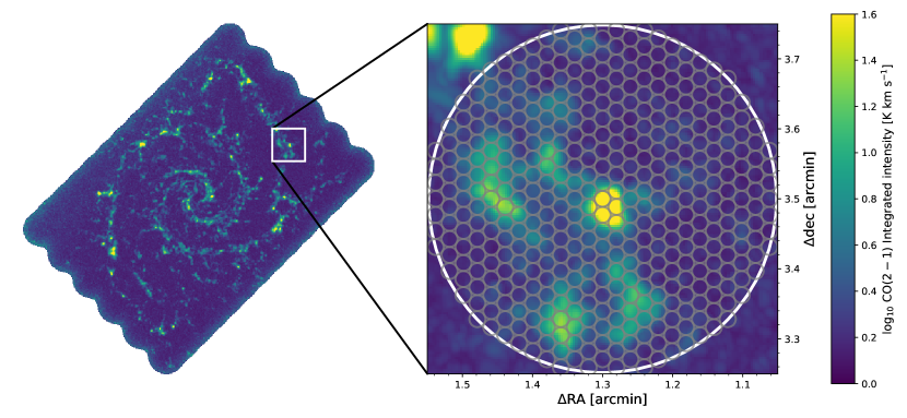
Figure 1: Left: CO(2–1) integrated intensity map of NGC 628 at $60$ pc resolution (color codes in the range of $0.0\leq{\rm log}_{10}$[CO(2–1)/K km s^-1] $\leq 1.6$). We use this map to estimate molecular gas surface density and free-fall time. Right: Illustration of our cross-scale methodology. We measure the molecular gas depletion time, $\tau_{\rm dep}\equiv\mbox{$\Sigma_{\rm mol}$}/\Sigma_{\rm SFR}$ at $1.3$ kpc resolution (illustrated by the large circle). Within each $1.3$ kpc region, we calculate $\Sigma_{\rm mol}$ and $\tau_{\rm ff}$ for each 60 pc beam (small circles). We average these high resolution $\tau_{\rm ff}$ estimates within 1.3 kpc region, weighted by $\Sigma_{\rm mol}$ at 60 pc beam. By dividing $\tau_{\rm ff}$ by $\tau_{\rm dep}^{\rm mol}$, we calculate the average $\epsilon_{\rm ff}$ within each $1.3$ kpc region while still leveraging the high resolution of the PHANGS-ALMA CO maps.

We calculate the mass-weighted mean of $\tau_{\rm ff}$^-1 via

$$\left<\tau_{\rm ff,60pc}^{-1}\right>_{\rm 1.3kpc}=\frac{\tau_{\rm ff,60pc}^{-1}~{}\mbox{$\Sigma_{\rm mol,60pc}$}~{}\ast~{}\theta_{\rm 60pc}^{\rm 1.3kpc}}{\Sigma_{\rm mol,60pc}~{}\ast~{}\theta_{\rm 60pc}^{\rm 1.3kpc}},$$ (9)

where $\Sigma_{\rm mol,60pc}$ is the surface density of molecular gas at $60$ pc resolution, $\theta_{\rm 60pc}^{\rm 1.3kpc}$ is the Gaussian kernel to convolve a $60$ pc resolution map to $1.3$ kpc resolution, and $\ast$ denotes convolution. We have round Gaussian beams in all maps. Hereby, we assume that $\left<\tau_{\rm ff,60pc}\right>_{\rm 1.3kpc}^{-1}\approx\left<\tau_{\rm ff,60pc}^{-1}\right>_{\rm 1.3kpc}$.

This differs slightly from Leroy et al. (2017a). They first calculated the mass-weighted mean of surface density, and then used that to calculate $\tau_{\rm ff}$, instead of directly calculating the mass-weighted mean of $\mbox{$\tau_{\rm ff}$}^{-1}$. The approach here should yield a more rigorous comparison to predictions in which $\Sigma_{\rm SFR}=\mbox{$\epsilon_{\rm ff}$}\ \Sigma_{\rm mol}/\mbox{$\tau_{\rm ff}$}$. The two approaches yield qualitatively similar results, though, with the mean $\left<\mbox{$\tau_{\rm ff}$}_{\rm,60pc}\right>_{\rm 1.3kpc}$ differing by only $\sim 7\%$.

3.5 Star Formation Efficiency per Free Fall Time

We calculate $\epsilon_{\rm ff}$ as the ratio between $\tau_{\rm ff}$ and $\tau_{\rm dep}^{\rm mol}$,

$$\mbox{$\left<\epsilon_{\rm ff,60pc}\right>_{\rm 1.3kpc}$}=\frac{\left<\tau_{\rm ff,60pc}\right>_{\rm 1.3kpc}}{\mbox{$\tau_{\rm dep,\,1.3kpc}^{\rm mol}$}}.$$ (10)

We carry out analogous calculations at 80, 100, and 120 pc resolutions. This allows us to study the impact of varying the linear resolution on the measured values of $\epsilon_{\rm ff}$. Our targets vary in their native physical resolutions, so not all targets are available at the highest resolutions (Sun et al., 2018).

3.6 Correction for Incompleteness

When estimating $\left<\mbox{$\tau_{\rm ff}$}_{\rm,60pc}\right>_{\rm 1.3kpc}$, we begin with a high resolution map that has been masked using a signal-to-noise cut (Sun et al., 2018). The calculation will miss emission at signal-to-noise below this cut, which has preferentially low $\Sigma_{\rm mol}$ and long $\tau_{\rm ff}$. Sun et al. (2018) measured the degree of this effect for each of our maps. They define the completeness, $C$, as the fraction of the total CO flux, measured at lower resolution with very good signal-to-noise, that is included in the high resolution, masked map. For our targets, $C$ ranges from 44% to 96% at 120 pc resolution, and is typically lower at finer resolutions.

To estimate the effect of incompleteness on our calculated $\tau_{\rm ff}$, we use a Monte Carlo approach. We randomly draw $10^{6}$ samples from a lognormal distribution designed to simulate the true distribution of mass as a function of $\Sigma_{\rm mol}$ (see Leroy et al., 2016; Sun et al., 2018). These model distributions have $1\sigma$ width of $0.5$ dex. For each distribution, we calculate true expectation value of $\mbox{$\tau_{\rm ff}$}^{-1}$ weighted by $\Sigma_{\rm mol}$, for the whole distribution and for subsets of the sample where only the highest fraction $C$ of the data are included.

This yields a correction factor $f_{C}$, defined as the ratio of the true $\left<\tau_{\rm ff}\right>$ over the measured $\left<\tau_{\rm ff}\right>$, as a function of $C$. We apply these to the data based on the value of $C$ measured in each $1.3$ kpc larger beam (our flux recovery is nearly perfect at $1.3$ kpc resolution; Leroy et al., 2016; Sun et al., 2018). Incompleteness suppresses faint, long $\tau_{\rm ff}$ lines-of-sight, so that $1.0\lesssim f_{C}\lesssim 1.1$ for 120 pc beam. Therefore, correcting for incompleteness increases $\tau_{\rm ff}$ and $\epsilon_{\rm ff}$.

4 Results

In the left panel of Figure 2 and Table 1, we summarize our measurements of $\epsilon_{\rm ff}$ for the whole sample, using our standard assumption ($H=100$ pc, SFR from FUV$+22\micron$, incomplete, and Galactic $\alpha_{\rm CO}$). These measurements over a large area across $14$ galaxies represent the most complete measurement of the efficiency of star formation per free fall time to date. At $120$ pc resolution (red histogram), we find median $\mbox{$\epsilon_{\rm ff}$}\approx 0.7\%$ across all lines-of-sight in $14$ galaxies, with the $16{-}84\%$ percentile range spanning $\mbox{$\epsilon_{\rm ff}$}\approx 0.4{-}1.1\%$.

The number of lines-of-sight varies in each galaxy. If instead, we take a median value for each galaxy, and compute the overall median across the whole sample (equivalent to giving equal weight to each galaxy), then $\mbox{$\epsilon_{\rm ff}$}\approx 0.8\%$. Those $\epsilon_{\rm ff}$ values are the most fundamental result of this letter.

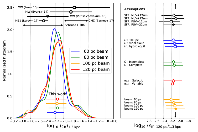
Figure 2: Efficiency per free fall time in 14 galaxies. Left: histograms of $\epsilon_{\rm ff}$ for all regions studied (smoothed using a Gaussian kernel density estimator following Scott 1992). The histograms combine all galaxies and give equal weight to each $1.3$ kpc region regardless of galaxy or other properties. Different colors show results for $\tau_{\rm ff}$ calculated at different resolutions. Circles and lines mark the median, 16^th, and $84^{\rm th}$ percentile $\epsilon_{\rm ff}$ for each resolution. For comparison, we show the values of $\epsilon_{\rm ff}$ measured for Milky Way clouds (Evans et al., 2014; Lee et al., 2016), in the Central Molecular Zone (Barnes et al., 2017), in M51 at 40 pc resolution (Leroy et al., 2017a), and a compilation study for MW and 7 nearby galaxies (Schruba et al. 2018b). Right: Impact of assumptions and uncertainties. We plot the median and $16^{\rm th}-84^{\rm th}$ percentile range of $\left<\mbox{$\epsilon_{\rm ff}$}\right>$ by altering various assumptions from our default values at 120 pc resolution. For various linear resolutions, we only include 9 galaxies that can be resolved down to 60 pc. Most systematic uncertainties affect the results at the $\sim 0.1$ dex ($\sim 25\%)$ level. The choices of SFR tracers and beam sizes have the largest impact. We also plot the median $\left<\mbox{$\epsilon_{\rm ff}$}\right>$, giving equal weight for each galaxy, as small vertical arrows.

Table 1: Measurements summary for all lines-of-sight.

	Physical resolutions of CO maps
Quantities	60 pc	80 pc	100 pc	120 pc
Numbers of galaxies	9	9	11	14
Numbers of lines-of-sight	949	949	1651	2937
Median of $\left<\epsilon_{\rm ff}\right>$	$0.63\%$	$0.72\%$	$0.70\%$	$0.71\%$
16th percentile of $\left<\epsilon_{\rm ff}\right>$	$0.40\%$	$0.44\%$	$0.38\%$	$0.39\%$
84th percentile of $\left<\epsilon_{\rm ff}\right>$	$1.00\%$	$1.15\%$	$1.15\%$	$1.15\%$
Median of $\left<\tau_{\rm ff}\right>$ [Myr]	11.16	12.68	12.54	11.79
16th percentile of $\left<\tau_{\rm ff}\right>$ [Myr]	6.52	7.04	7.29	7.57
84th percentile of $\left<\tau_{\rm ff}\right>$ [Myr]	13.62	15.74	15.75	15.59
Median of $\tau_{\rm dep}$ [Gyr]	1.72	1.72	1.77	1.69
16th percentile of $\tau_{\rm dep}$ [Gyr]	1.18	1.18	1.13	1.11
84th percentile of $\tau_{\rm dep}$ [Gyr]	2.29	2.29	2.41	2.35

4.1 Uncertainties

The histograms in Figure 2 combine more than $940$ regions of 1.3 kpc in size (see Table 1), and the statistical uncertainties on any given $\epsilon_{\rm ff}$ estimate tend to be quite small ($\lesssim 0.01$ dex), because many measurements are already averaged together within each $1.3$ kpc beam. As a result, we expect that the spread in the histogram to represent real physical variations in $\epsilon_{\rm ff}$ from region to region and from galaxy to galaxy. The dominant uncertainties affecting the measurement are systematic. We explore the magnitude of these systematic uncertainties in the right panel of Figure 2, where we vary our adopted SFR tracer, the line-of-sight depth, completeness correction, the CO-to-H₂ conversion factor, and linear resolution.

In general, over the range of assumptions that we explore, systematic effects can shift $\epsilon_{\rm ff}$ by $\sim 0.1$ dex. In particular, altering our mix of SFR tracers shifts $\epsilon_{\rm ff}$ by $\lesssim 0.1$ dex. Adopting a metallicity-dependent $\alpha_{\rm CO}$ only has a small impact on the median $\epsilon_{\rm ff}$ of the whole sample because our low mass galaxies contribute only a small fraction of the total lines-of-sight. However, variations in $\alpha_{\rm CO}$ have a more significant impact on the measured $\epsilon_{\rm ff}$ in individual galaxies ($\S$4.3).

Varying the resolution of the maps changes $\epsilon_{\rm ff}$, but only weakly. Within our sample, changing the resolution from 60 to 120 pc increases $\epsilon_{\rm ff}$ by $\sim 0.1$ dex. This is consistent with the idea that beam dilution decreases the measured $\Sigma_{\rm mol}$ as the resolution degrades, which in turn raises $\tau_{\rm ff}$ and $\epsilon_{\rm ff}$. Other systematic uncertainties stem from imperfect knowledge of the disk thickness, $H$, and incompleteness due to limited sensitivity in the high resolution CO maps. The right panel of Figure 2 shows that correcting for the presence of low $\Sigma_{\rm mol}$, high $\tau_{\rm ff}$ lines-of-sight shifts $\epsilon_{\rm ff}$ towards higher value by $<0.1$ dex. Meanwhile, adopting different plausible treatments of $H$ can also shift $\epsilon_{\rm ff}$ by $\lesssim 0.1$ dex. Direct measurements of the vertical distribution of the cold gas in galaxies (Yim et al., 2011, 2014) will help to constraint $H$ and $\epsilon_{\rm ff}$.

4.2 Comparison to Previous Studies

We find $\mbox{$\epsilon_{\rm ff}$}\approx 0.7\%\pm 0.3\%$. This value is comparable to the often-quoted theoretical values of $\approx 1\%$ (McKee & Ostriker, 2007; Krumholz & Tan, 2007; Krumholz et al., 2012). Numerical simulations of kpc-scale regions of the ISM with star formation feedback found $\epsilon_{\rm ff}$ $\approx~{}0.6\%$ (Kim et al., 2013); this can be understood based on expectations from UV heating and turbulence driving by supernovae (Ostriker et al., 2010; Ostriker & Shetty, 2011). Our $\epsilon_{\rm ff}$ value is lower than $\mbox{$\epsilon_{\rm ff}$}\approx 10\%$ suggested by Agertz & Kravtsov (2015), but they also argued that their high local efficiency is derived from a short cloud-scale $\tau_{\rm dep}^{\rm mol}$ (rather than kpc-scales as in our work), and can still result in a low apparent global efficiency ($\sim 0.25\%$) if a global (kpc-scales) $\tau_{\rm dep}^{\rm mol}$ of $\sim 2$ Gyrs (Leroy et al., 2013; Utomo et al., 2017, this work) is adopted.

As Figure 2 shows, our measured $\epsilon_{\rm ff}$ is low compared to the median $\epsilon_{\rm ff}$ $\sim 1.5{-}1.8\%$ found in the Milky Way (MW) clouds by Evans et al. (2014), Lee et al. (2016), and Barnes et al. (2017). This can be partially understood because the focus of MW measurements is on the high column density parts of clouds (Evans et al., 2014) and on actively star forming clouds (Lee et al., 2016). Evans et al. measured $\epsilon_{\rm ff}$ within a visual extinction contour of $A_{V}>2$ magnitude (equivalent to $\Sigma_{\rm mol}\gtrsim 20~{}M_{\odot}$ pc^-2). Our measurements also integrate over lower column density regions, resulting in $\tau_{\rm ff}$ and $\tau_{\rm dep}^{\rm mol}$ $\sim 8$ and 16 times longer than those in Evans et al. Indeed, Vutisalchavakul et al. (2016) found a mean $\mbox{$\epsilon_{\rm ff}$}\approx 0.4\%$ by considering a sample of lower volume density of MW clouds (with mean $n_{\rm H2}\sim 300$ cm^-3, instead of $800$ cm^-3 as in Evans et al.).

Furthermore, we expect the difference with the Lee et al. (2016) MW measurements to reflect a bias towards actively star forming clouds in their sample (e.g., Kruijssen & Longmore, 2014; Kruijssen et al., 2018, §2.1). Their measurements include $\sim 80\%$ of the ionizing photon flux in the MW, but only captured $\sim 10\%$ of the total GMC mass in the Miville-Deschênes et al. (2017) catalog. Our measurements include all CO emission in each 1.3 kpc aperture, so that clouds and star forming regions in all evolutionary states are included (as long as they are above the sensitivity limit). Following Murray (2011), Lee et al. (2016) emphasized the large scatter of $\epsilon_{\rm ff}$ from cloud to cloud (a result that goes back to Mooney & Solomon, 1988). Our 1.3 kpc $\tau_{\rm dep}^{\rm mol}$ measurements average over many clouds and so neither contradict nor confirm their result. Cloud-by-cloud star formation rate estimates are in progress for PHANGS (e.g., K. Kreckel et al. in preparation), and will help to test whether the observations of Murray (2011) and Lee et al. (2016) indeed hold in other galaxies.

Our median $\mbox{$\epsilon_{\rm ff}$}\approx 0.7\%$ in the whole sample is about twice the $\mbox{$\epsilon_{\rm ff}$}\approx 0.30-0.36\%$ found by Leroy et al. (2017a) using an almost identical methodology to study M51 at 40 pc resolution. M51 is also part of our sample, and our measurements for that galaxy agree well with those in Leroy et al. (2017a). This appears to reflect a real difference between M51 and the rest of our sample, i.e. M51 has the lowest $\epsilon_{\rm ff}$ of any galaxy in our sample. Following Meidt et al. (2013), this may reflect strong gas flows in M51 that act to stabilize the gas and suppress star formation. Strong gas flows were also observed in NGC 3627 (Beuther et al., 2017), where $\epsilon_{\rm ff}$ is low ($\approx 0.6\%$).

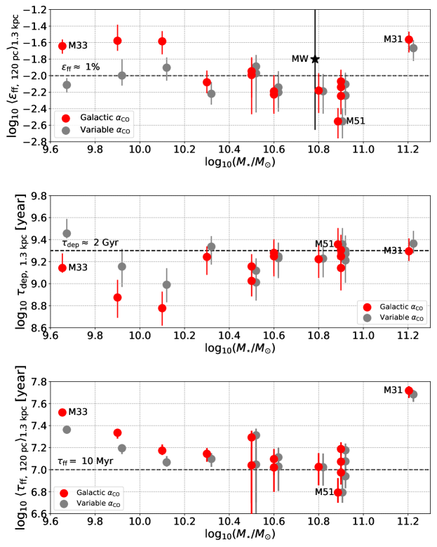
Figure 3: Galaxy-by-galaxy measurements of $\epsilon_{\rm ff}$, $\tau_{\rm dep}^{\rm mol}$, and $\tau_{\rm ff}$. Top panel: Median and $16^{\rm th}-84^{\rm th}$ percentile range of $\epsilon_{\rm ff}$ for each galaxy as a function of galaxy stellar mass ($M_{*}$) for Galactic $\alpha_{\rm CO}$ (red circles and bars) and a metallicity-dependent $\alpha_{\rm CO}$ (gray circles and bars). We shift the gray circles to the right by 0.02 dex for clarity. Middle and bottom panels: same as the top panel, but for $\tau_{\rm dep}^{\rm mol}$ and $\tau_{\rm ff}$.

4.3 Galaxy-to-Galaxy Variations

Figure 2 shows overall results for the whole sample, but we also observe strong galaxy-to-galaxy variations in $\epsilon_{\rm ff}$. In Figure 3 and Table 2, we report $\epsilon_{\rm ff}$ for each galaxy at 120 pc resolution. Red circles and bars show the median and $16^{\rm th}{-}84^{\rm th}$ percentile range for each galaxy using a Galactic $\alpha_{\rm CO}$. Here, the contrast between low mass, low metallicity galaxies and massive galaxies stands out. To illuminate a possible cause for this, we also show results adopting metallicity-dependent $\alpha_{\rm CO}$ as gray circles. Because $\epsilon_{\rm ff}$ depends on both $\tau_{\rm dep}^{\rm mol}$ and $\tau_{\rm ff}$, we also plot these quantities in the middle and lower panels.

The top panel of Figure 3 shows a dynamic range of an order of magnitude in $\epsilon_{\rm ff}$ ($\approx 0.3$–$2.6\%$) across our sample. Among the high mass galaxies (excluding M31 and M51), the scatter in $\epsilon_{\rm ff}$ is $\sim 0.2$ dex. Except for M31, $\epsilon_{\rm ff}$ appears to decrease with increasing stellar mass of the galaxy (Spearman rank correlation coefficient, $r_{s}\approx-0.75$).

The middle and bottom panels show that this trend originates from a combination of changes in $\tau_{\rm dep}^{\rm mol}$ and $\tau_{\rm ff}$. For Galactic $\alpha_{\rm CO}$, our three lowest mass galaxies show the shortest $\tau_{\rm dep}^{\rm mol}$ in our sample ($\lesssim 1$ Gyr). A similar $\tau_{\rm dep}^{\rm mol}$$-M_{\star}$ trend was also observed by Saintonge et al. (2011), Leroy et al. (2013), and Bolatto et al. (2017). Meanwhile, $\tau_{\rm ff}$ declines with increasing stellar mass ($r_{s}\approx-0.64$; excluding M31). This agrees with the observation that at a fixed resolution, $\Sigma_{\rm mol}$ scales with galaxy stellar mass (Sun et al., 2018), leading to longer $\tau_{\rm ff}$ in low mass galaxies.

Much, but not all, of the observed trends with stellar mass can be explained by the application of a metallicity dependent $\alpha_{\rm CO}$, shown as the gray points. If a large reservoir of CO-dark molecular gas is present in these low mass galaxies (e.g., Leroy et al., 2011; Bolatto et al., 2013; Gratier et al., 2017; Schruba et al., 2017), then $\tau_{\rm dep}^{\rm mol}$ will be longer and $\tau_{\rm ff}$ shorter, resulting in lower $\epsilon_{\rm ff}$ in the low mass galaxies. The correction that we adopt, which is uncertain, yields $\mbox{$\epsilon_{\rm ff}$}\sim 1\%$ in the low mass targets, similar to $\epsilon_{\rm ff}$ in the high mass galaxies. However, even with this metallicity correction, there is still a significant anti-correlation between galaxy stellar mass and $\epsilon_{\rm ff}$ ($r_{s}\approx-0.57$; excluding M31).

M31 shows a higher $\epsilon_{\rm ff}$ that can not be explained by the metallicity-dependent $\alpha_{\rm CO}$ only. This apparent high efficiency may partially reflect beam-filling effects. M31 has a low molecular-to-atomic gas fraction, and if the clouds are small, widely spaced, and tenuous compared to the beam (as suggested by Sun et al. 2018), then the long $\tau_{\rm ff}$ may be partially an observational bias due to low beam filling factor.

5 Summary

We estimate the star formation efficiency per gravitational free-fall time, $\epsilon_{\rm ff}$, in $14$ star-forming galaxies, where $11$ of them are part of the PHANGS-ALMA survey. This represents the most complete measurement of this key theoretical quantity across local galaxies to date. To do so, we use high resolution CO maps to infer the molecular gas volume density and free-fall time, $\tau_{\rm ff}$, at $60{-}120$ pc resolution. We estimate the gas depletion time from the same CO maps and archival UV and IR data, convolved to $1.3$ kpc resolution. We connect those cross-scale measurements by taking the mass-weighted average of $\tau_{\rm ff}$^-1 within 1.3 kpc aperture.

Overall, we find $\epsilon_{\rm ff}$ in the range of $0.4{-}1.1\%$, with median $\approx 0.7\%$, and significant galaxy-to-galaxy scatter ($0.3-2.6\%$). We assess the impact of systematic uncertainties on this measurement to be within $0.1$ dex, with the largest uncertainties associated with the assumption of molecular gas thickness and the choice of SFR tracer. The galaxy-to-galaxy scatter in $\epsilon_{\rm ff}$ is systematic, with an overall trend toward finding higher $\epsilon_{\rm ff}$ in low mass galaxies and in our only “green valley” target, M31. We argue that these trends may be partially explained by a metallicity-dependent $\alpha_{\rm CO}$ and sparse, small clouds in M31.

Table 2: Measurements for each galaxy at 120 pc beam of CO maps.

Galaxies	Morphology	distance	inclination	log${}_{10}M_{*}$	log10SFR	# l.o.s	log10$\tau_{\rm ff}$	log10$\tau_{\rm dep}^{\rm mol}$	log10$\epsilon_{\rm ff}$	$C$	$f_{C}$	$\alpha_{\rm CO}$(1–0)
		Mpc	degree	$M_{\odot}$	$M_{\odot}$ yr-1		years	years				(see notes)
NGC 0224	Sb-A	0.8	77.7	11.20	$-0.43$	22	$7.72_{-0.06(-0.30)}^{+0.03(+0.18)}$	$9.29_{-0.08(-0.14)}^{+0.11(+0.07)}$	$-1.56_{-0.15(-0.05)}^{+0.09(+0.65)}$	$0.97_{-0.05}^{+0.10}$	$1.01_{-0.01}^{+0.01}$	$5.10$
NGC 6744	Sbc-AB	11.6	40.0	10.90	$0.39$	299	$7.19_{-0.05(-0.02)}^{+0.05(+0.04)}$	$9.25_{-0.10(-0.06)}^{+0.11(+0.02)}$	$-2.07_{-0.10(-0.00)}^{+0.13(+0.16)}$	$0.67_{-0.17}^{+0.15}$	$1.05_{-0.02}^{+0.02}$	$4.59$
NGC 4321	Sbc-AB	15.2	27.0	10.90	$0.53$	525	$7.07_{-0.15(-0.00)}^{+0.09(+0.04)}$	$9.31_{-0.15(-0.06)}^{+0.13(+0.07)}$	$-2.25_{-0.22(-0.04)}^{+0.20(+0.14)}$	$0.65_{-0.31}^{+0.19}$	$1.05_{-0.03}^{+0.05}$	$4.29$
NGC 4303	Sbc-AB	17.6	25.0	10.90	$0.72$	424	$6.97_{-0.10(-0.03)}^{+0.08(+0.08)}$	$9.14_{-0.20(-0.06)}^{+0.14(+0.07)}$	$-2.14_{-0.23(-0.11)}^{+0.18(+0.13)}$	$0.75_{-0.26}^{+0.13}$	$1.03_{-0.02}^{+0.04}$	$5.10$
NGC 5194	Sbc-A	7.6	21.0	10.89	$0.43$	100	$6.79_{-0.09(-0.00)}^{+0.12(+0.08)}$	$9.36_{-0.13(-0.05)}^{+0.14(+0.10)}$	$-2.55_{-0.20(-0.10)}^{+0.15(+0.14)}$	$0.90_{-0.17}^{+0.06}$	$1.01_{-0.01}^{+0.02}$	$4.35$
NGC 4254	Sc-A	16.8	27.0	10.80	$0.68$	553	$7.03_{-0.16(-0.00)}^{+0.12(+0.08)}$	$9.22_{-0.17(-0.05)}^{+0.12(+0.05)}$	$-2.18_{-0.26(-0.05)}^{+0.20(+0.13)}$	$0.76_{-0.26}^{+0.15}$	$1.03_{-0.02}^{+0.04}$	$4.41$
NGC 4535	Sc-AB	15.8	40.0	10.60	$0.30$	314	$7.10_{-0.14(-0.00)}^{+0.08(+0.07)}$	$9.28_{-0.18(-0.06)}^{+0.12(+0.06)}$	$-2.19_{-0.24(-0.00)}^{+0.19(+0.20)}$	$0.63_{-0.16}^{+0.15}$	$1.05_{-0.02}^{+0.03}$	$4.04$
NGC 3627	Sb-AB	8.3	62.0	10.60	$0.10$	153	$7.02_{-0.22(-0.04)}^{+0.11(+0.19)}$	$9.25_{-0.18(-0.05)}^{+0.14(+0.13)}$	$-2.23_{-0.23(-0.00)}^{+0.19(+0.40)}$	$0.89_{-0.10}^{+0.06}$	$1.02_{-0.01}^{+0.01}$	$4.18$
NGC 3351	Sb-B	10.0	41.0	10.50	$0.11$	93	$7.29_{-0.71(-0.08)}^{+0.05(+0.02)}$	$9.16_{-0.27(-0.08)}^{+0.11(+0.12)}$	$-1.95_{-0.31(-0.06)}^{+0.13(+0.24)}$	$0.76_{-0.12}^{+0.16}$	$1.03_{-0.02}^{+0.02}$	$3.98$
NGC 1672	Sb-B	11.9	40.0	10.50	$0.48$	172	$7.04_{-0.34(-0.02)}^{+0.15(+0.10)}$	$9.03_{-0.14(-0.06)}^{+0.13(+0.13)}$	$-1.99_{-0.47(-0.09)}^{+0.21(+0.22)}$	$0.69_{-0.19}^{+0.17}$	$1.04_{-0.02}^{+0.03}$	$4.21$
NGC 0628	Sc-A	9.0	6.5	10.30	$-0.02$	208	$7.14_{-0.07(-0.05)}^{+0.05(+0.05)}$	$9.24_{-0.16(-0.06)}^{+0.09(+0.09)}$	$-2.08_{-0.13(-0.16)}^{+0.13(+0.10)}$	$0.80_{-0.10}^{+0.06}$	$1.03_{-0.01}^{+0.01}$	$5.39$
NGC 5068	Scd-AB	9.0	26.9	10.10	$-0.59$	30	$7.17_{-0.03(-0.11)}^{+0.05(+0.07)}$	$8.78_{-0.15(-0.08)}^{+0.15(+0.21)}$	$-1.58_{-0.15(-0.31)}^{+0.12(+0.15)}$	$0.60_{-0.08}^{+0.05}$	$1.06_{-0.01}^{+0.01}$	$7.10$
NGC 2835	Sc-B	10.1	56.4	9.90	$-0.40$	23	$7.34_{-0.05(-0.14)}^{+0.02(+0.04)}$	$8.87_{-0.18(-0.07)}^{+0.16(+0.28)}$	$-1.58_{-0.12(-0.25)}^{+0.19(+0.27)}$	$0.44_{-0.11}^{+0.08}$	$1.08_{-0.01}^{+0.02}$	$8.30$
NGC 0598	Scd-A	0.9	58.0	9.65	$-0.35$	19	$7.52_{-0.03(-0.29)}^{+0.02(+0.06)}$	$9.14_{-0.04(-0.00)}^{+0.13(+0.31)}$	$-1.64_{-0.09(-0.45)}^{+0.07(+0.22)}$	$0.85_{-0.05}^{+0.04}$	$1.02_{-0.01}^{+0.01}$	$8.95$

Note. — Aliases for NGC 224, NGC 598, and NGC 5194 are M31, M33, and M51, respectively. The values of $\tau_{\rm ff}$, $\tau_{\rm dep}^{\rm mol}$, and $\epsilon_{\rm ff}$ are for SFR(FUV+22µm), $H=100$ pc, $C<1$, and Galactic $\alpha_{\rm CO}$. We provide the scatter of measurements ($+/-$ sign) as the range between 16th and 84th percentiles. The systematic uncertainties, defined as the largest difference between the median quantities from various assumptions, are written inside the parentheses. The standard errors of the median are very small ($\lesssim 0.01$ dex), and so not reported. Units of metallicity dependent $\alpha_{\rm CO}$(1–0) are $M_{\odot}$ [K km s^-1 pc²]^-1.

References

- Agertz & Kravtsov (2015) Agertz, O., & Kravtsov, A. V. 2015, ApJ, 804, 18
- Barnes et al. (2017) Barnes, A. T., Longmore, S. N., Battersby, C., et al. 2017, MNRAS, 469, 2263
- Bertoldi & McKee (1992) Bertoldi, F., & McKee, C. F. 1992, ApJ, 395, 140
- Beuther et al. (2017) Beuther, H., Meidt, S., Schinnerer, E., Paladino, R., & Leroy, A. 2017, A&A, 597, A85
- Bigiel et al. (2016) Bigiel, F., Leroy, A. K., Jiménez-Donaire, M. J., et al. 2016, ApJ, 822, L26
- Bolatto et al. (2013) Bolatto, A. D., Wolfire, M., & Leroy, A. K. 2013, ARA&A, 51, 207
- Bolatto et al. (2017) Bolatto, A. D., Wong, T., Utomo, D., et al. 2017, ApJ, 846, 159
- Caldú-Primo & Schruba (2016) Caldú-Primo, A., & Schruba, A. 2016, AJ, 151, 34
- Croxall et al. (2015) Croxall, K. V., Pogge, R. W., Berg, D. A., Skillman, E. D., & Moustakas, J. 2015, ApJ, 808, 42
- Druard et al. (2014) Druard, C., Braine, J., Schuster, K. F., et al. 2014, A&A, 567, A118
- Evans et al. (2014) Evans, II, N. J., Heiderman, A., & Vutisalchavakul, N. 2014, ApJ, 782, 114
- Federrath (2015) Federrath, C. 2015, MNRAS, 450, 4035
- Federrath & Klessen (2012) Federrath, C., & Klessen, R. S. 2012, ApJ, 761, 156
- Gallagher et al. (2018) Gallagher, M. J., Leroy, A. K., Bigiel, F., et al. 2018, ApJ in press, arXiv:1803.10785, arXiv:1803.10785
- Gao & Solomon (2004a) Gao, Y., & Solomon, P. M. 2004a, ApJS, 152, 63
- Gao & Solomon (2004b) —. 2004b, ApJ, 606, 271
- García-Burillo et al. (2012) García-Burillo, S., Usero, A., Alonso-Herrero, A., et al. 2012, A&A, 539, A8
- Gratier et al. (2017) Gratier, P., Braine, J., Schuster, K., et al. 2017, A&A, 600, A27
- Heyer & Dame (2015) Heyer, M., & Dame, T. M. 2015, ARA&A, 53, 583
- Jarrett et al. (2013) Jarrett, T. H., Masci, F., Tsai, C. W., et al. 2013, AJ, 145, 6
- Kennicutt & Evans (2012) Kennicutt, R. C., & Evans, N. J. 2012, ARA&A, 50, 531
- Kim et al. (2013) Kim, C.-G., Ostriker, E. C., & Kim, W.-T. 2013, ApJ, 776, 1
- Kruijssen & Longmore (2014) Kruijssen, J. M. D., & Longmore, S. N. 2014, MNRAS, 439, 3239
- Kruijssen et al. (2014) Kruijssen, J. M. D., Longmore, S. N., Elmegreen, B. G., et al. 2014, MNRAS, 440, 3370
- Kruijssen et al. (2018) Kruijssen, J. M. D., Schruba, A., Hygate, A. P. S., et al. 2018, MNRAS in press, arXiv:1805.00012
- Krumholz (2014) Krumholz, M. R. 2014, Phys. Rep., 539, 49
- Krumholz et al. (2012) Krumholz, M. R., Dekel, A., & McKee, C. F. 2012, ApJ, 745, 69
- Krumholz & McKee (2005) Krumholz, M. R., & McKee, C. F. 2005, ApJ, 630, 250
- Krumholz & Tan (2007) Krumholz, M. R., & Tan, J. C. 2007, ApJ, 654, 304
- Lang (2014) Lang, D. 2014, AJ, 147, 108
- Lee et al. (2016) Lee, E. J., Miville-Deschênes, M.-A., & Murray, N. W. 2016, ApJ, 833, 229
- Leroy et al. (2011) Leroy, A. K., Bolatto, A., Gordon, K., et al. 2011, ApJ, 737, 12
- Leroy et al. (2013) Leroy, A. K., Walter, F., Sandstrom, K., et al. 2013, AJ, 146, 19
- Leroy et al. (2016) Leroy, A. K., Hughes, A., Schruba, A., et al. 2016, ApJ, 831, 16
- Leroy et al. (2017a) Leroy, A. K., Schinnerer, E., Hughes, A., et al. 2017a, ApJ, 846, 71
- Leroy et al. (2017b) Leroy, A. K., Usero, A., Schruba, A., et al. 2017b, ApJ, 835, 217
- Longmore et al. (2013) Longmore, S. N., Bally, J., Testi, L., et al. 2013, MNRAS, 429, 987
- Makarov et al. (2014) Makarov, D., Prugniel, P., Terekhova, N., Courtois, H., & Vauglin, I. 2014, A&A, 570, A13
- Martin & GALEX Team (2005) Martin, C., & GALEX Team. 2005, in IAU Symposium, Vol. 216, Maps of the Cosmos, ed. M. Colless, L. Staveley-Smith, & R. A. Stathakis, 221
- McKee & Ostriker (2007) McKee, C. F., & Ostriker, E. C. 2007, ARA&A, 45, 565
- Meidt et al. (2013) Meidt, S. E., Schinnerer, E., García-Burillo, S., et al. 2013, ApJ, 779, 45
- Meidt et al. (2014) Meidt, S. E., Schinnerer, E., van de Ven, G., et al. 2014, ApJ, 788, 144
- Meidt et al. (2018) Meidt, S. E., Leroy, A. K., Rosolowsky, E., et al. 2018, ApJ, 854, 100
- Miville-Deschênes et al. (2017) Miville-Deschênes, M.-A., Murray, N., & Lee, E. J. 2017, ApJ, 834, 57
- Mooney & Solomon (1988) Mooney, T. J., & Solomon, P. M. 1988, ApJ, 334, L51
- Murray (2011) Murray, N. 2011, ApJ, 729, 133
- Murray et al. (2010) Murray, N., Quataert, E., & Thompson, T. A. 2010, ApJ, 709, 191
- Ochsendorf et al. (2017) Ochsendorf, B. B., Meixner, M., Roman-Duval, J., Rahman, M., & Evans, II, N. J. 2017, ApJ, 841, 109
- Ostriker et al. (2010) Ostriker, E. C., McKee, C. F., & Leroy, A. K. 2010, ApJ, 721, 975
- Ostriker & Shetty (2011) Ostriker, E. C., & Shetty, R. 2011, ApJ, 731, 41
- Padoan et al. (2012) Padoan, P., Haugbølle, T., & Nordlund, Å. 2012, ApJ, 759, L27
- Peek & Schiminovich (2013) Peek, J. E. G., & Schiminovich, D. 2013, ApJ, 771, 68
- Pety et al. (2013) Pety, J., Schinnerer, E., Leroy, A. K., et al. 2013, ApJ, 779, 43
- Pilyugin et al. (2004) Pilyugin, L. S., Vílchez, J. M., & Contini, T. 2004, A&A, 425, 849
- Querejeta et al. (2015) Querejeta, M., Meidt, S. E., Schinnerer, E., et al. 2015, ApJS, 219, 5
- Raskutti et al. (2016) Raskutti, S., Ostriker, E. C., & Skinner, M. A. 2016, ApJ, 829, 130
- Rosolowsky & Simon (2008) Rosolowsky, E., & Simon, J. D. 2008, ApJ, 675, 1213
- Saintonge et al. (2011) Saintonge, A., Kauffmann, G., Wang, J., et al. 2011, MNRAS, 415, 61
- Sakamoto et al. (1997) Sakamoto, S., Hasegawa, T., Handa, T., Hayashi, M., & Oka, T. 1997, ApJ, 486, 276
- Sandstrom et al. (2013) Sandstrom, K. M., Leroy, A. K., Walter, F., et al. 2013, ApJ, 777, 5
- Schinnerer et al. (2013) Schinnerer, E., Meidt, S. E., Pety, J., et al. 2013, ApJ, 779, 42
- Schlegel et al. (1998) Schlegel, D. J., Finkbeiner, D. P., & Davis, M. 1998, ApJ, 500, 525
- Schruba et al. (2017) Schruba, A., Leroy, A. K., Kruijssen, J. M. D., et al. 2017, ApJ, 835, 278
- Scott (1992) Scott, D. W. 1992, Multivariate Density Estimation
- Sun et al. (2018) Sun, J., Leroy, A. K., Schruba, A., et al. 2018, ArXiv e-prints, arXiv:1805.00937
- Tully et al. (2009) Tully, R. B., Rizzi, L., Shaya, E. J., et al. 2009, AJ, 138, 323
- Usero et al. (2015) Usero, A., Leroy, A. K., Walter, F., et al. 2015, AJ, 150, 115
- Utomo et al. (2017) Utomo, D., Bolatto, A. D., Wong, T., et al. 2017, ApJ, 849, 26
- Vutisalchavakul et al. (2016) Vutisalchavakul, N., Evans, II, N. J., & Heyer, M. 2016, ApJ, 831, 73
- Yim et al. (2011) Yim, K., Wong, T., Howk, J. C., & van der Hulst, J. M. 2011, AJ, 141, 48
- Yim et al. (2014) Yim, K., Wong, T., Xue, R., et al. 2014, AJ, 148, 127