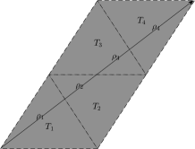
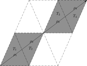
A Posteriori Error Estimate and Adaptive Mesh Refinement Algorithm for Atomistic/Continuum Coupling with Finite Range Interactions in Two Dimensions

M. Liao Mingjie Liao
Department of Applied Mathematics and Mechanics
University of Science and Technology Beijing
No. 30 Xueyuan Road, Haidian District
Beijing 100083
China
mliao@xs.ustb.edu.cn
P. Lin Ping Lin
Department of Mathematics
University of Dundee
Dundee, DD1 4HN, Scotland
United Kingdom
plin@maths.dundee.ac.uk
 and  L. Zhang Lei Zhang
School of Mathematical Sciences, Institute of Natural Sciences, and Ministry of Education Key Laboratory of Scientific and Engineering Computing (MOE-LSC)
Shanghai Jiao Tong University
800 Dongchuan Road
Shanghai 200240
China
lzhang2012@sjtu.edu.cn
Abstract.

In this paper, we develop the residual based a posteriori error estimates and the corresponding adaptive mesh refinement algorithm for atomistic/continuum (a/c) coupling with finite range interactions in two dimensions. We have systematically derived a new explicitly computable stress tensor formula for finite range interactions. In particular, we use the geometric reconstruction based consistent atomistic/continuum (GRAC) coupling scheme, which is optimal if the continuum model is discretized by P1superscript𝑃1P^{1} finite elements. The numerical results of the adaptive mesh refinement algorithm is consistent with the optimal a priori error estimates.

Key words and phrases:
atomistic models, coarse graining, atomistic-to-continuum coupling, quasicontinuum method, a posteriori error estimate
2000 Mathematics Subject Classification:
65N12, 65N15, 70C20, 82D25
ML and PL were partially supported by National Natural Science Foundation of China grant 91430106. LZ was partially supported by National Natural Science Foundation of China grant 11471214, 11571314 and the One Thousand Plan of China for young scientists.

1. Introduction

Atomistic/continuum (a/c) coupling methods are a class of computational multiscale methods for crystalline solids with defects that aim to optimally balance the accuracy of the atomistic model and the efficiency of the continuum model [19, 35, 11]. The construction and analysis of different a/c coupling methods have attracted considerable attention in the research community in recent years. Rigorous a prior analysis and systematic benchmark has been done in, for example, [14, 24, 12, 29, 30, 15]. We refer readers to [18, 16] for a review. The study of a/c coupling methods has not only provided an analytical framework for the prototypical problems[9], but also opened avenue for coupling schemes in more complicated physical situations [3, 4, 13].

Like many multiscale methods dealing with defects or singularities, adaptivity is the key for the efficient implementation of a/c coupling methods. In contrast to the a priori analysis, the development of a posteriori analysis for a/c coupling methods are still lagging behind. Although heuristic methods have been proposed in the engineering literature [39, 32, 35]. Previous mathematical justifications are largely limited to one dimension cases [32, 1, 2]. In particular, the residual based a posteriori error bounds for a/c coupling schemes are first derived in [25, 20, 27] by Ortner et al. in one dimension.

In [40], we carried out a rigorous a posteriori analysis of the residual, the stability constant, and the error bound, for a consistent atomistic/continuum coupling method [28] with nearest neighbour interactions in two dimensions. Corresponding adaptive mesh refinement algorithm was designed and implemented based on the a posteriori error estimates, and the convergence rate with respect to degrees of freedom is the same as optimal a priori error estimates. This is the first rigorous a posteriori analysis for a/c coupling method in two dimensions. With the a posteriori error estimates and the adaptive algorithm, we can not only automatically move the a/c interface and adjust the discretization of the continuum region, but also change the size of the computational domain. We have also introduced the so-called “stress tensor correction” technique, which distinguish the essential difference of high dimensional results compared with previous one dimensional results.

In this paper, we treat the more general case of a/c coupling with finite range interactions, which is physically more relevant and computationally more involved. The a priori analysis of GRAC scheme has been extended from nearest neighbour case in [28] to finite range interactions in [29]. 1superscript1\ell^{1}-minimization is introduced to resolve the issue of non-uniqueness of reconstruction parameters, and a stabilisation mechanism is proposed in [22] to reduce the stability gap between the a/c coupling scheme and the original atomistic model.

The analytical framework for both a priori analysis and a posteriori analysis of a/c coupling methods strongly relies on the stress based formulation. In [21, 26], an explicit formulation of stress tensor is proposed based on a mollified version of line measure supported on the interaction bonds, thence one can obtain an integral representation of finite differences to further derive an integral representation of the first variation of the interaction energy. This representation greatly simplifies the expression of the stress tensor and plays a significant role in the a priori analysis. However, the obtained stress tensor is a function of the continuous space variable, therefore it is difficult to compute in practice, and not suitable for the a posteriori estimates and adaptive computation.

In this paper, we derive a novel expression of the stress tensor for finite range interactions, which is new to the best of our knowledge. The stress tensor is piecewise constant and only depends on a local neighbourhood, therefore it is computable and the assembly cost is linear with respect to the number of bonds. This stress formulation allows for the convenient derivation of a posterior error estimates and efficient implementation of the adaptive algorithms.

The paper is organized as follows. We set up the atomistic to continuum (a/c) coupling models for point defects in § 2, and introduce the general GRAC formulation in § 3. In § 4, we present the stress formulation and the stress tensor assembly algorithm for finite range interactions. In § 5 the rigorous a posteriori error estimates based adaptive algorithm is deduced and complemented by numerical experiments. We draw conclusions and make suggestions for future research in § 6. Some auxiliary results are given in the Appendix § 7.

2. Model Formulation

In this section, We setup an atomistic model for crystal defects in an infinite lattice in the spirit of [9] in § 2.1 and then introduce the Cauchy-Born continuum model in § 2.2. We give a generic form of a/c coupling schemes in § 2.3.

2.1. Atomistic Model

2.1.1. Atomistic lattice and defects

Given d{2,3}𝑑23d\in\{2,3\}, Ad×dAsuperscript𝑑𝑑{\textsf{A}}\in\mathbb{R}^{d\times d} non-singular, Λhom:=AdassignsuperscriptΛhomAsuperscript𝑑\Lambda^{\textrm{hom}}:={\textsf{A}}\mathbb{Z}^{d} is the homogeneous reference lattice which represents a perfect single lattice crystal formed by identical atoms. ΛdΛsuperscript𝑑\Lambda\subset\mathbb{R}^{d} is the reference lattice with some local defects. The mismatch between ΛΛ\Lambda and ΛhomsuperscriptΛhom\Lambda^{\textrm{hom}} represents possible defects ΛdefsuperscriptΛdef\Lambda^{\textrm{def}}, which are contained in some localized defect cores Ddefsuperscript𝐷defD^{\textrm{def}} such that the atoms in ΛDdefΛsuperscript𝐷def\Lambda\setminus D^{\textrm{def}} do not interact with defects ΛdefsuperscriptΛdef\Lambda^{\textrm{def}}. Vacancy, interstitial and impurity are different types of possible point defects.

2.1.2. Lattice function and lattice function space

Given m{1,2,3}𝑚123m\in\{1,2,3\}, denote the set of vector-valued lattice functions by

𝒰:={v:Λm}.assign𝒰conditional-set𝑣Λsuperscript𝑚\mathscr{U}:=\{v:\Lambda\to\mathbb{R}^{m}\}.

A deformed configuration is a lattice function y𝒰𝑦𝒰y\in\mathscr{U}. Let x𝑥x be the identity map, the displacement u𝒰𝑢𝒰u\in\mathscr{U} is defined by u()=y()x()=y()𝑢𝑦𝑥𝑦u(\ell)=y(\ell)-x(\ell)=y(\ell)-\ell for any ΛΛ\ell\in\Lambda.

For each ΛΛ\ell\in\Lambda, we prescribe an interaction neighbourhood 𝒩:={Λ| 0<||rcut}assignsubscript𝒩conditional-setsuperscriptΛ 0superscriptsubscript𝑟cut\mathcal{N}_{\ell}:=\{\ell^{\prime}\in\Lambda\,|\,0<|\ell^{\prime}-\ell|\leq r_{\textrm{cut}}\} with some cut-off radius rcutsubscript𝑟cutr_{\textrm{cut}}. The interaction range :={|𝒩}assignsubscriptconditional-setsuperscriptsuperscriptsubscript𝒩\mathcal{R}_{\ell}:=\{\ell^{\prime}-\ell\,|\,\ell^{\prime}\in\mathcal{N}_{\ell}\} is defined as the union of lattice vectors defined by the finite differences between lattice points in 𝒩subscript𝒩\mathcal{N}_{\ell} and \ell. Define the “finite difference stencil” Dv():={Dρv()}ρ:={v(+ρ)v()}ρassign𝐷𝑣subscriptsubscript𝐷𝜌𝑣𝜌subscriptassignsubscript𝑣𝜌𝑣𝜌subscriptDv(\ell):=\{D_{\rho}v(\ell)\}_{\rho\in\mathcal{R}_{\ell}}:=\{v(\ell+\rho)-v(\ell)\}_{\rho\in\mathcal{R}_{\ell}}.

The homogeneous lattice Λhom=AdsuperscriptΛhomAsuperscript𝑑\Lambda^{\textrm{hom}}={\textsf{A}}\mathbb{Z}^{d} naturally induces a simplicial micro-triangulation 𝒯asuperscript𝒯a\mathcal{T}^{\textrm{a}}. In two dimensions, 𝒯a={Aξ+T^,AξT^|ξ2}superscript𝒯aconditional-setA𝜉^𝑇A𝜉^𝑇𝜉superscript2\mathcal{T}^{\textrm{a}}=\{{\textsf{A}}\xi+\hat{T},{\textsf{A}}\xi-\hat{T}|\xi\in\mathbb{Z}^{2}\}, where T^=conv{0,e1,e2}^𝑇conv0subscript𝑒1subscript𝑒2\hat{T}={\textrm{conv}}\{0,e_{1},e_{2}\}. Let ζ¯W1,(Λhom;)¯𝜁superscript𝑊1superscriptΛhom\bar{\zeta}\in W^{1,\infty}(\Lambda^{\textrm{hom}};\mathbb{R}) be the P1subscript𝑃1P_{1} nodal basis function associated with the origin; namely, ζ¯¯𝜁\bar{\zeta} is piecewise linear with respect to 𝒯asuperscript𝒯a\mathcal{T}^{\textrm{a}}, and ζ¯(0)=1¯𝜁01\bar{\zeta}(0)=1 and ζ¯(ξ)=0¯𝜁𝜉0\bar{\zeta}(\xi)=0 for ξ0𝜉0\xi\neq 0 and ξΛhom𝜉superscriptΛhom\xi\in\Lambda^{\textrm{hom}}. The nodal interpolant of v𝒰𝑣𝒰v\in\mathscr{U} can be written as

v¯(x):=ξdv(ξ)ζ¯(xξ).assign¯𝑣𝑥subscript𝜉superscript𝑑𝑣𝜉¯𝜁𝑥𝜉\bar{v}(x):=\sum_{\xi\in\mathbb{Z}^{d}}v(\xi)\bar{\zeta}(x-\xi).

We can introduce the discrete homogeneous Sobolev spaces

𝒰1,2:={u𝒰|u¯L2},assignsuperscript𝒰12conditional-set𝑢𝒰¯𝑢superscript𝐿2\mathscr{U}^{1,2}:=\{u\in\mathscr{U}|\nabla\bar{u}\in L^{2}\},

with semi-norm u¯L2subscriptnorm¯𝑢superscript𝐿2\|\nabla\bar{u}\|_{L^{2}}.

2.1.3. Interaction potential

We consider the general multibody interaction potential of the generic pair functional form [38], which includes the widely used potentials such as EAM (Embedded Atom Method) potential [5] and Finnis-Sinclair model [10]. Namely, the potential is a function of the distances between atoms within interaction range and has no angular dependence. For example, for each ΛΛ\ell\in\Lambda, let V(y)subscript𝑉𝑦V_{\ell}(y) denote the site energy associated with the lattice site ΛΛ\ell\in\Lambda, the EAM potential reads,

V(y):=assignsubscript𝑉𝑦absent\displaystyle V_{\ell}(y):= 𝒩Φ(|y()y()|)+F(𝒩ψ(|y()y()|)),subscriptsuperscriptsubscript𝒩Φ𝑦𝑦superscript𝐹subscriptsuperscriptsubscript𝒩𝜓𝑦𝑦superscript\displaystyle\sum_{\ell^{\prime}\in\mathcal{N}_{\ell}}\Phi(|y(\ell)-y(\ell^{\prime})|)+F\Big{(}{\textstyle\sum_{\ell^{\prime}\in\mathcal{N}_{\ell}}\psi(|y(\ell)-y(\ell^{\prime})|)}\Big{)},
=\displaystyle= ρΦ(|Dρy()|)+F(ρψ(|Dρy()|)).subscript𝜌subscriptΦsubscript𝐷𝜌𝑦𝐹subscript𝜌subscript𝜓subscript𝐷𝜌𝑦\displaystyle\sum_{\rho\in\mathcal{R}_{\ell}}\Phi\big{(}|D_{\rho}y(\ell)|\big{)}+F\Big{(}{\textstyle\sum_{\rho\in\mathcal{R}_{\ell}}}\psi\big{(}|D_{\rho}y(\ell)|\big{)}\Big{)}. (2.1)

with the pair potential ΦΦ\Phi, the electron density function ψ𝜓\psi and the embedding function F𝐹F.


Remark 2.1. For convenience, with a slight abuse of notation, we will use V(Dρy)subscript𝑉subscript𝐷𝜌𝑦V_{\ell}(D_{\rho}y), V(|Dρy|)subscript𝑉subscript𝐷𝜌𝑦V_{\ell}(|D_{\rho}y|) instead of V^({Dρy()}ρ)subscript^𝑉subscriptsubscript𝐷𝜌𝑦𝜌subscript\widehat{V}_{\ell}(\{D_{\rho}y(\ell)\}_{\rho\in\mathcal{R}_{\ell}}), V~({|Dρy()|}ρ)subscript~𝑉subscriptsubscript𝐷𝜌𝑦𝜌subscript\widetilde{V}_{\ell}(\{|D_{\rho}y(\ell)|\}_{\rho\in\mathcal{R}_{\ell}}) when there is no confusion in the context. ∎

We assume that the potential V(y)Ck((d)),k2formulae-sequencesubscript𝑉𝑦superscript𝐶𝑘superscriptsuperscript𝑑subscript𝑘2V_{\ell}(y)\in C^{k}((\mathbb{R}^{d})^{\mathcal{R}_{\ell}}),k\geq 2. We also assume that V(y)subscript𝑉𝑦V_{\ell}(y) is homogeneous outside the defect region Ddefsuperscript𝐷defD^{\textrm{def}}, namely, V=Vsubscript𝑉𝑉V_{\ell}=V and =subscript\mathcal{R}_{\ell}=\mathcal{R} for ΛDdefΛsuperscript𝐷def\ell\in\Lambda\setminus D^{\textrm{def}}. Furthermore, V𝑉V and \mathcal{R} have the following point symmetry: =\mathcal{R}=-\mathcal{R}, and V({gρ}ρ)=V(g)𝑉subscriptsubscript𝑔𝜌𝜌𝑉𝑔V(\{-g_{-\rho}\}_{\rho\in\mathcal{R}})=V(g).

For an infinite lattice, assume the macroscopic applied strain is Bd×dBsuperscript𝑑𝑑\textsf{B}\in\mathbb{R}^{d\times d}, we redefine the potential V(y)subscript𝑉𝑦V_{\ell}(y) as the difference V(y)V(yB)subscript𝑉𝑦subscript𝑉subscript𝑦BV_{\ell}(y)-V_{\ell}(y_{\textsf{B}}). We denote the energy functional (y)𝑦\mathscr{E}(y) as the infinite sum of the redefined potential over ΛΛ\Lambda, which is well-defined for yyB𝒰1,2𝑦superscript𝑦Bsuperscript𝒰12y-y^{\textsf{B}}\in\mathscr{U}^{1,2} [9],

(y)=ΛV(y)𝑦subscriptΛsubscript𝑉𝑦\mathscr{E}(y)=\sum_{\ell\in\Lambda}V_{\ell}(y) (2.2)

Under the above conditions, the goal of the atomistic problem is to find a strongly stable equilibrium y𝑦y, such that,

yargmin{(y)|yyB𝒰1,2}.𝑦conditional𝑦𝑦superscript𝑦𝐵superscript𝒰12y\in\arg\min\big{\{}\mathscr{E}(y)\,\big{|}\,y-y^{B}\in\mathscr{U}^{1,2}\big{\}}. (2.3)

y𝑦y is strongly stable if there exists c0>0subscript𝑐00c_{0}>0 such that

δ2(y)v,vc0vL22,v𝒰1,2.formulae-sequencesuperscript𝛿2𝑦𝑣𝑣subscript𝑐0superscriptsubscriptnorm𝑣superscript𝐿22for-all𝑣superscript𝒰12\langle\delta^{2}\mathscr{E}(y)v,v\rangle\geq c_{0}\|\nabla v\|_{L^{2}}^{2},\quad\forall v\in\mathscr{U}^{1,2}.

2.2. Continuum model

From the atomistic model, a continuum model can be derived by coarse graining, and computationally it allows for the reduction of degrees of freedom when the deformation is smooth. A typical choice in the multi-scale context is the Cauchy-Born continuum model [8, 26]. Let W:d×d:𝑊superscript𝑑𝑑W:\mathbb{R}^{d\times d}\to\mathbb{R} be a strain energy density function, the Cauchy-Born energy density W𝑊W is defined by

W(F):=detA1V(F).assign𝑊FsuperscriptA1𝑉FW(\textsf{F}):=\det{\textsf{A}}^{-1}V(\textsf{F}\cdot\mathcal{R}).

2.3. Generic Formulation of Energy Based Atomistic/Continuum Coupling

We give a generic formulation of the a/c coupling method and employ concepts and notation from various earlier works, such as [19, 35, 36, 17, 29], and we adapt the formulation to the settings in this paper.

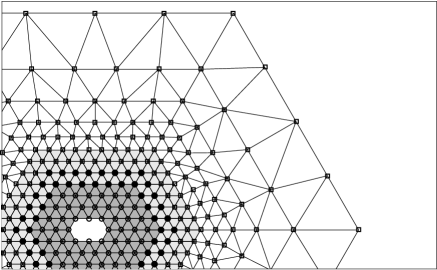
The computational domain ΩR=ΩRaΩRcdsubscriptΩ𝑅superscriptsubscriptΩ𝑅asuperscriptsubscriptΩ𝑅csuperscript𝑑\Omega_{R}=\Omega_{R}^{\textrm{a}}\bigcup\Omega_{R}^{\textrm{c}}\subset\mathbb{R}^{d} is a simply connected, polygonal and closed set, consists of the atomistic region ΩRasuperscriptsubscriptΩ𝑅a\Omega_{R}^{\textrm{a}} and the continuum partition ΩRcsuperscriptsubscriptΩ𝑅c\Omega_{R}^{\textrm{c}}, where R𝑅R is the radius of ΩRsubscriptΩ𝑅\Omega_{R}. Given the reference lattice ΛΛ\Lambda with some local defects, we decompose the set Λa,i:=ΛΩRa=ΛaΛiassignsuperscriptΛaiΛsubscriptsuperscriptΩa𝑅superscriptΛasuperscriptΛi\Lambda^{\textrm{a},\textrm{i}}:=\Lambda\bigcap\Omega^{\textrm{a}}_{R}=\Lambda^{\textrm{a}}\bigcup\Lambda^{\textrm{i}} into a core atomistic set ΛasuperscriptΛa\Lambda^{\textrm{a}} and an interfacial atomistic set ΛisuperscriptΛi\Lambda^{\textrm{i}} such that ΛDdefΛaΛsuperscript𝐷defsuperscriptΛa\Lambda\bigcap D^{\textrm{def}}\subset\Lambda^{\textrm{a}}, where Ddefsuperscript𝐷defD^{\textrm{def}} represents the defect core. Let 𝒯h,Rasubscriptsuperscript𝒯a𝑅\mathcal{T}^{\textrm{a}}_{h,R} (respectively 𝒯h,Risubscriptsuperscript𝒯i𝑅\mathcal{T}^{\textrm{i}}_{h,R}) be the canonical triangulation induced by ΛasuperscriptΛa\Lambda^{\textrm{a}} (respectively ΛisuperscriptΛi\Lambda^{\textrm{i}}), and 𝒯h,Rcsubscriptsuperscript𝒯𝑐𝑅\mathcal{T}^{c}_{h,R} be a shape-regular simplicial partition of the continuum region. We denote 𝒯h,R=𝒯h,Rc𝒯h,Ri𝒯h,Rasubscript𝒯𝑅subscriptsuperscript𝒯c𝑅subscriptsuperscript𝒯i𝑅subscriptsuperscript𝒯a𝑅{\mathcal{T}_{h,R}}=\mathcal{T}^{\textrm{c}}_{h,R}\bigcup\mathcal{T}^{\textrm{i}}_{h,R}\bigcup\mathcal{T}^{\textrm{a}}_{h,R} as the triangulation of the a/c coupling configuration. Please see Figure 1 for an illustration of the computational mesh.
Refer to caption
Figure 1. Illustration of computational mesh. The computational domain is ΩRsubscriptΩ𝑅\Omega_{R}, and the corresponding triangulation is 𝒯h,Rsubscript𝒯𝑅\mathcal{T}_{h,R}. \circ in the DimGrey region are atoms of ΛasuperscriptΛ𝑎\Lambda^{a}. For the next nearest neighbour interaction, ΛisuperscriptΛi\Lambda^{\textrm{i}} contains \bullet in the LightGrey interface region. \Box are continuum degrees of freedom.

The space of coarse-grained displacements is,

𝒰h,R:={uh:Ωh,Rm|\displaystyle\mathscr{U}_{h,R}:=\big{\{}u_{h}:\Omega_{h,R}\to\mathbb{R}^{m}\,\big{|}\,~{} uhsubscript𝑢u_{h} is continuous and p.w. affine w.r.t. 𝒯h,Rsubscript𝒯𝑅\mathcal{T}_{h,R},
uh=0 on ΩR }.\displaystyle\text{ $u_{h}=0$ on $\partial\Omega_{R}$ }\big{\}}.

The subscript R𝑅R in the above definitions can be dropped if there is no confusion, for example, we can replace 𝒯h,Rsubscript𝒯𝑅{\mathcal{T}_{h,R}} by 𝒯hsubscript𝒯h\mathcal{T}_{\textrm{h}}.

Let vor()vor\textrm{vor}(\ell) represents the voronoi cell associated with \ell of the homogeneous reference lattice Λhom:=AdassignsuperscriptΛhomAsuperscript𝑑\Lambda^{\textrm{hom}}:={\textsf{A}}\mathbb{Z}^{d}, for some given non-singular Ad×dAsuperscript𝑑𝑑{\textsf{A}}\in\mathbb{R}^{d\times d}. We have |vor()|=detAvorA|\textrm{vor}(\ell)|=\det{\textsf{A}}, for each ΛhomsuperscriptΛhom\ell\in\Lambda^{\textrm{hom}}. For each ΛΛ\ell\in\Lambda denote its effective cell as νsubscript𝜈\nu_{\ell} (see [28]), let ω:=|ν||vor()|assignsubscript𝜔subscript𝜈vor\omega_{\ell}:=\displaystyle{\frac{|\nu_{\ell}|}{|\textrm{vor}(\ell)|}} be the effective volume associated with \ell. For each element T𝒯h𝑇subscript𝒯hT\in\mathcal{T}_{\textrm{h}} we define the effective volume of T𝑇T by

ωT:=|T(Λavor())(Λiνi)|.assignsubscript𝜔𝑇𝑇subscriptsuperscriptΛavorsubscriptsuperscriptΛisubscriptsuperscript𝜈i\omega_{T}:=|T\setminus(\bigcup_{\ell\in\Lambda^{\textrm{a}}}{\textrm{vor}}(\ell))\setminus(\bigcup_{\ell\in\Lambda^{\textrm{i}}}\nu^{\textrm{i}}_{\ell})|.

We note that ωT=0subscript𝜔𝑇0\omega_{T}=0 if T𝒯ha𝒯hi𝑇subscriptsuperscript𝒯asubscriptsuperscript𝒯iT\in\mathcal{T}^{\textrm{a}}_{h}\setminus\mathcal{T}^{\textrm{i}}_{h}, ωT=|T|subscript𝜔𝑇𝑇\omega_{T}=|T| if T𝒯hc𝒯hi𝑇subscriptsuperscript𝒯csubscriptsuperscript𝒯iT\in\mathcal{T}^{\textrm{c}}_{h}\setminus\mathcal{T}^{\textrm{i}}_{h}, and 0ωT<|T|0subscript𝜔𝑇𝑇0\leq\omega_{T}<|T| if T𝒯hi𝑇subscriptsuperscript𝒯iT\in\mathcal{T}^{\textrm{i}}_{h}, dependes on how we defining νisuperscriptsubscript𝜈𝑖\nu_{\ell}^{i}, the effective cell of ΛisuperscriptΛ𝑖\ell\in\Lambda^{i}. The choices of νsubscript𝜈\nu_{\ell} and ωTsubscript𝜔𝑇\omega_{T} satisfy Λa,iν+T𝒯hωT=|Ωh,R|subscriptsuperscriptΛaisubscript𝜈subscript𝑇subscript𝒯hsubscript𝜔𝑇subscriptΩ𝑅\sum_{\ell\in\Lambda^{\textrm{a},\textrm{i}}}\nu_{\ell}+\sum_{T\in\mathcal{T}_{\textrm{h}}}\omega_{T}=|\Omega_{h,R}|.

Now we are ready to define the generic a/c coupling energy functional hsuperscripth\mathscr{E}^{\textrm{h}},

h(yh):=assignsuperscripthsubscript𝑦absent\displaystyle\mathscr{E}^{\textrm{h}}(y_{h}):= ΛaV(yh)+ΛiωVi(yh)+T𝒯hωTW(yh|T)subscriptsuperscriptΛasubscript𝑉subscript𝑦subscriptsuperscriptΛisubscript𝜔subscriptsuperscript𝑉isubscript𝑦subscript𝑇subscript𝒯hsubscript𝜔𝑇𝑊evaluated-atsubscript𝑦𝑇\displaystyle\sum_{\ell\in\Lambda^{\textrm{a}}}V_{\ell}(y_{h})+\sum_{\ell\in\Lambda^{\textrm{i}}}\omega_{\ell}V^{\textrm{i}}_{\ell}(y_{h})+\sum_{T\in\mathcal{T}_{\textrm{h}}}\omega_{T}W(\nabla y_{h}|_{T}) (2.4)

where Visuperscriptsubscript𝑉iV_{\ell}^{\textrm{i}} is a modified interface site potential.

The goal of a/c coupling is to find

yh,Rargmin{h(yh)|yhyB𝒰h,R}.subscript𝑦𝑅conditionalsuperscripthsubscript𝑦subscript𝑦superscript𝑦𝐵subscript𝒰𝑅y_{h,R}\in\arg\min\big{\{}\mathscr{E}^{\textrm{h}}(y_{h})\,\big{|}\,y_{h}-y^{B}\in\mathscr{U}_{h,R}\big{\}}. (2.5)

The subscript R𝑅R in yh,Rsubscript𝑦𝑅y_{h,R} and 𝒰h,Rsubscript𝒰𝑅\mathscr{U}_{h,R} can be omitted if there is no confusion.

The first variation of the a/c coupling variational problem (2.5) is to find yhyB𝒰h,Rsubscript𝑦superscript𝑦Bsubscript𝒰𝑅y_{h}-y^{\textsf{B}}\in\mathscr{U}_{h,R} such that

δh(yh),vh=0,vh𝒰h,R.formulae-sequence𝛿superscripthsubscript𝑦subscript𝑣0for-allsubscript𝑣subscript𝒰𝑅\langle\delta\mathscr{E}^{\textrm{h}}(y_{h}),v_{h}\rangle=0,\quad\forall v_{h}\in\mathscr{U}_{h,R}. (2.6)

Spurious artificial force could occur at the interface for energy based coupling even for homogeneous deformation [35], and was dubbed ”ghost force”. The issue of ”ghost force removal” has received considerable attention in the recent years, and consistent a/c coupling methods without ghost force were developed by [36, 7] in one dimension and [28, 33] in two dimensions. We will introduce the consistent GRAC formulation in § 3 .

3. General GRAC formulation

In this section, we describe the construction of the geometric reconstruction based consistent atomistic/continuum (GRAC) coupling energy for multibody potentials with general interaction range and arbitrary interfaces.

Given the homogeneous site potential V(Dy())𝑉𝐷𝑦V\big{(}Dy(\ell)\big{)}, we can represent the interface potential Visuperscriptsubscript𝑉iV_{\ell}^{\textrm{i}} in (2.4) in terms of V𝑉V. For each Λi,ρ,ςformulae-sequencesuperscriptΛi𝜌𝜍subscript\ell\in\Lambda^{\textrm{i}},\rho,\varsigma\in\mathcal{R}_{\ell}, let C;ρ,ςsubscript𝐶𝜌𝜍C_{\ell;\rho,\varsigma} be free parameters, and define

Vi(y):=V((ςC;ρ,ςDςy())ρ)assignsuperscriptsubscript𝑉i𝑦𝑉subscriptsubscript𝜍subscriptsubscript𝐶𝜌𝜍subscript𝐷𝜍𝑦𝜌subscriptV_{\ell}^{\textrm{i}}(y):=V\Big{(}\big{(}{\textstyle\sum_{\varsigma\in\mathcal{R}_{\ell}}C_{\ell;\rho,\varsigma}D_{\varsigma}y(\ell)}\big{)}_{\rho\in\mathcal{R}_{\ell}}\Big{)} (3.1)

A convenient short-hand notation is

Vi(y)=V(CDy()),where{C:=(C;ρ,ς)ρ,ς,andCDy:=(ςC;ρ,ςDςy)ρ.superscriptsubscript𝑉i𝑦𝑉subscript𝐶𝐷𝑦wherecasesassignsubscript𝐶subscriptsubscript𝐶𝜌𝜍𝜌𝜍subscriptandmissing-subexpressionassignsubscript𝐶𝐷𝑦subscriptsubscript𝜍subscriptsubscript𝐶𝜌𝜍subscript𝐷𝜍𝑦𝜌subscriptmissing-subexpressionV_{\ell}^{\textrm{i}}(y)=V(C_{\ell}\cdot Dy(\ell)),\quad\text{where}\quad\left\{\begin{array}[]{rl}C_{\ell}:=(C_{\ell;\rho,\varsigma})_{\rho,\varsigma\in\mathcal{R}_{\ell}},\quad\text{and}&\\ C_{\ell}\cdot Dy:=\big{(}{\textstyle\sum_{\varsigma\in\mathcal{R}_{\ell}}C_{\ell;\rho,\varsigma}D_{\varsigma}y}\big{)}_{\rho\in\mathcal{R}_{\ell}}.&\end{array}\right.

We call the parameters C;ρ,ςsubscript𝐶𝜌𝜍C_{\ell;\rho,\varsigma} as the reconstruction parameters.

To construct consistent a/c coupling energy, we need to enforce the so-called patch tests for the energy functional hsuperscripth\mathscr{E}^{\textrm{h}}, namely, energy patch test (3.2) and force patch test (3.4). Those patch tests in turn prescribe conditions (3.3) and (3.6) for the reconstruction parameters C𝐶C. In general, the reconstruction parameters satisfying patch tests are not unique, an 1superscript1\ell^{1}-minimization technique can be introduced to choose the ”optimal” parameters [29]. Also, a stabilisation mechanism can be applied to improve the stability of the GRAC coupling scheme [22].

3.1. Energy patch test

To guarantee that hsuperscripth\mathscr{E}^{\textrm{h}} approximates the atomistic energy =ΛV(y)subscriptΛsubscript𝑉𝑦\mathscr{E}=\sum_{\ell\in\Lambda}V_{\ell}(y), it is reasonable to require that the interface potentials satisfy an energy patch test

Vi(yF)=V(yF)Λi,Fm×d.formulae-sequencesuperscriptsubscript𝑉isuperscript𝑦F𝑉superscript𝑦Fformulae-sequencefor-allsuperscriptΛiFsuperscript𝑚𝑑V_{\ell}^{\textrm{i}}(y^{\textsf{F}})=V(y^{\textsf{F}})\qquad\quad\forall\ell\in\Lambda^{\textrm{i}},\quad\textsf{F}\in\mathbb{R}^{m\times d}. (3.2)

namely, the interface potential coincides with the atomistic potential for uniform deformations.

For the GRAC coupling scheme, a sufficient and necessary condition for the energy patch test is that F()=C(F)Fsubscript𝐶F\textsf{F}\cdot\mathcal{R}(\ell)=C_{\ell}\cdot(\textsf{F}\cdot\mathcal{R}) for all Fm×dFsuperscript𝑚𝑑\textsf{F}\in\mathbb{R}^{m\times d} and ΛisuperscriptΛi\ell\in\Lambda^{\textrm{i}}. This is equivalent to

ρ=ς()C;ρ,ςςΛi,ρ().formulae-sequence𝜌subscript𝜍subscript𝐶𝜌𝜍𝜍formulae-sequencefor-allsuperscriptΛi𝜌\rho=\sum_{\varsigma\in\mathcal{R}(\ell)}C_{\ell;\rho,\varsigma}\varsigma\qquad\forall\ell\in\Lambda^{\textrm{i}},\quad\rho\in\mathcal{R}(\ell). (3.3)

3.2. Force patch test

We call the following condition the force patch test, namely, for Λ=ΛhomΛsuperscriptΛhom\Lambda=\Lambda^{\textrm{hom}} and Φ=ΦsubscriptΦΦ\Phi_{\ell}=\Phi,

δh(yF),vh=0vh𝒰h,Fm×d.formulae-sequence𝛿superscripthsuperscript𝑦Fsubscript𝑣0formulae-sequencefor-allsubscript𝑣subscript𝒰Fsuperscript𝑚𝑑\langle\delta\mathscr{E}^{\textrm{h}}(y^{\textsf{F}}),v_{h}\rangle=0\qquad\forall v_{h}\in\mathscr{U}_{h},\quad\textsf{F}\in\mathbb{R}^{m\times d}. (3.4)

where F is some uniform deformation gradient. This is saying that there is no artificial ”ghost force” for uniform deformations.

From the general GRAC formulation (2.4), we can decompose the first variation of the a/c coupling energy into three parts,

δh(yF),vh=δa(yF),vh+δi(yF),vh+δc(yF),vh.vh𝒰h\langle\delta\mathscr{E}^{\textrm{h}}(y^{\textsf{F}}),v_{h}\rangle=\langle\delta\mathscr{E}^{\textrm{a}}(y^{\textsf{F}}),v_{h}\rangle+\langle\delta\mathscr{E}^{\textrm{i}}(y^{\textsf{F}}),v_{h}\rangle+\langle\delta\mathscr{E}^{\textrm{c}}(y^{\textsf{F}}),v_{h}\rangle.\quad\forall v_{h}\in\mathscr{U}_{h} (3.5)

To simplify the notation, we drop the yFsuperscript𝑦Fy^{\textsf{F}} dependence from the following expressions in this section, for example, we write asuperscripta\mathscr{E}^{\textrm{a}} instead of a(yF)superscriptasuperscript𝑦F\mathscr{E}^{\textrm{a}}(y^{\textsf{F}}), ρVsubscript𝜌𝑉\nabla_{\rho}V instead of ρV(DyF)subscript𝜌𝑉𝐷superscript𝑦F\nabla_{\rho}V(Dy^{\textsf{F}}), and so forth. Here, ρVsubscript𝜌𝑉\nabla_{\rho}V denotes the partial derivative of V𝑉V with respect to the Dρysubscript𝐷𝜌𝑦D_{\rho}y component. Since ρV=ρVsubscript𝜌𝑉subscript𝜌𝑉\nabla_{\rho}V=-\nabla_{-\rho}V, we only consider half of the directions in the interaction range: fix +superscript\mathcal{R}^{+}\subset\mathcal{R} such that +(+)=superscriptsuperscript\mathcal{R}^{+}\cup(-\mathcal{R}^{+})=\mathcal{R} and +(+)=superscriptsuperscript\mathcal{R}^{+}\cap(-\mathcal{R}^{+})=\emptyset.

As proposed in [29], a necessary and sufficient condition on the reconstruction parameters Csubscript𝐶C_{\ell} to satisfy the force patch test (3.4) for all VC((d))𝑉superscript𝐶superscriptsuperscript𝑑V\in C^{\infty}((\mathbb{R}^{d})^{\mathcal{R}}) is

cρa()+cρi()+cρc()=0,subscriptsuperscript𝑐a𝜌subscriptsuperscript𝑐i𝜌subscriptsuperscript𝑐c𝜌0c^{\textrm{a}}_{\rho}(\ell)+c^{\textrm{i}}_{\rho}(\ell)+c^{\textrm{c}}_{\rho}(\ell)=0, (3.6)

for Λi+superscriptΛi\ell\in\Lambda^{\textrm{i}}+\mathcal{R}, and ρ+𝜌superscript\rho\in\mathcal{R}^{+}. The coefficients cρa()subscriptsuperscript𝑐a𝜌c^{\textrm{a}}_{\rho}(\ell), cρi()subscriptsuperscript𝑐i𝜌c^{\textrm{i}}_{\rho}(\ell) and cρc()subscriptsuperscript𝑐c𝜌c^{\textrm{c}}_{\rho}(\ell) are geometric parameters with respect to the underlying lattice and the interface geometry, formulated by collecting all the coefficients for the terms ρV\nabla_{\rho}V\cdot of the first variations of a/c coupling energy as in the following equations (3.7). The interface coefficients cρi()subscriptsuperscript𝑐i𝜌c^{\textrm{i}}_{\rho}(\ell) depend linearly on the unknown reconstruction paramters C;ρ,ςsubscript𝐶𝜌𝜍C_{\ell;\rho,\varsigma}. Then, by (3.5), we have

δa,vh=Λa+ρ+cρa()[ρVvh()]=ρ+Λaρ[ρVvh()]ρ+Λa+ρ[ρVvh()],δi,vh=Λi+ρ+cρi()[ρVvh()]=ςΛi+ςωςiρ+(Cς;ρ,ςCς;ρ,ς)[ρVvh()]Λiωiρ+ς(C;ρ,ςC;ρ,ς)[ρVvh()],andδc,vh=Tρ+i=132ωTdetATϕiTρ[ρVvh,iT],=Tρ+i=132ωTdetATϕiTρ[ρVvh,iT],\displaystyle\begin{split}\langle\delta\mathscr{E}^{\textrm{a}},v_{h}\rangle&=\sum_{\ell\in\Lambda^{\textrm{a}}+\mathcal{R}}\sum_{\rho\in\mathcal{R}^{+}}c^{\textrm{a}}_{\rho}(\ell)\big{[}\nabla_{\rho}V\cdot v_{h}(\ell)\big{]}\\ &=\sum_{\begin{subarray}{c}\rho\in\mathcal{R}^{+}\\ \ell\in\Lambda^{\textrm{a}}-\rho\end{subarray}}{\big{[}\nabla_{\rho}V\cdot v_{h}(\ell)\big{]}}-\sum_{\begin{subarray}{c}\rho\in\mathcal{R}^{+}\\ \ell\in\Lambda^{\textrm{a}}+\rho\end{subarray}}\big{[}\nabla_{\rho}V\cdot v_{h}(\ell)\big{]},\\ \langle\delta\mathscr{E}^{\textrm{i}},v_{h}\rangle&=\sum_{\ell\in\Lambda^{i}+\mathcal{R}}\sum_{\rho\in\mathcal{R}^{+}}c^{\textrm{i}}_{\rho}(\ell)\big{[}\nabla_{\rho}V\cdot v_{h}(\ell)\big{]}\\ &=\sum_{\begin{subarray}{c}\varsigma\in\mathcal{R}\\ \ell\in\Lambda^{\textrm{i}}+\varsigma\end{subarray}}\omega_{\ell-\varsigma}^{\textrm{i}}\sum_{\rho\in\mathcal{R}^{+}}(C_{\ell-\varsigma;\rho,\varsigma}-C_{\ell-\varsigma;-\rho,\varsigma})\big{[}\nabla_{\rho}V\cdot v_{h}(\ell)\big{]}\\ &\qquad-\sum_{\ell\in\Lambda^{\textrm{i}}}\omega_{\ell}^{\textrm{i}}\sum_{\rho\in\mathcal{R}^{+}}\sum_{\varsigma\in\mathcal{R}}(C_{\ell;\rho,\varsigma}-C_{\ell;-\rho,\varsigma})\big{[}\nabla_{\rho}V\cdot v_{h}(\ell)\big{]},\quad\text{and}\\ \langle\delta\mathscr{E}^{\textrm{c}},v_{h}\rangle&=\sum_{T}\sum_{\rho\in\mathcal{R}^{+}}\sum_{i=1}^{3}2\frac{\omega_{T}}{\det{\textsf{A}}}\nabla_{T}\phi_{i}^{T}\cdot\rho\big{[}{\nabla_{\rho}V}\cdot v^{T}_{h,i}\big{]},\\ &=\sum_{T}\sum_{\rho\in\mathcal{R}^{+}}\sum_{i=1}^{3}2\frac{\omega_{T}}{\det{\textsf{A}}}\nabla_{T}\phi_{i}^{T}\cdot\rho\big{[}{\nabla_{\rho}V}\cdot v^{T}_{h,i}\big{]},\end{split} (3.7)

where the nodes iTsuperscriptsubscript𝑖𝑇\ell_{i}^{T} are the three corners of the triangle T𝑇T, vh,iT=v(iT)superscriptsubscript𝑣𝑖𝑇𝑣superscriptsubscript𝑖𝑇v_{h,i}^{T}=v(\ell_{i}^{T}) and ϕiTsuperscriptsubscriptitalic-ϕ𝑖𝑇\phi_{i}^{T} are the three nodal linear bases corresponding to vh,iTsuperscriptsubscript𝑣𝑖𝑇v_{h,i}^{T}, i=1,2,3𝑖123i=1,2,3,

The force patch test is automatically satisfied for the atomistic model and the Cauchy-Born continuum model.Therefore, we only need to consider the force consistency for those sites with the extended interface region Λi+:={Λ|Λi,ρ, such that =+ρ}assignsuperscriptΛiconditional-setΛformulae-sequencesuperscriptsuperscriptΛiformulae-sequence𝜌 such that superscript𝜌\Lambda^{\textrm{i}}+\mathcal{R}:=\{\ell\in\Lambda|\exists\ell^{\prime}\in\Lambda^{\textrm{i}},\exists\rho\in\mathcal{R},\text{ such that }\ell=\ell^{\prime}+\rho\}. Therefore (3.6) for Λi+superscriptΛi\ell\in\Lambda^{\textrm{i}}+\mathcal{R} together with (3.3) for ΛisuperscriptΛi\ell\in\Lambda^{\textrm{i}} form a linear system for the unknown parameters C;ρ,ςsubscript𝐶𝜌𝜍C_{\ell;\rho,\varsigma}.


Remark 3.1. In [28, 29], we choose ωi=vor(),Λiformulae-sequencesuperscriptsubscript𝜔𝑖vorfor-allsuperscriptΛ𝑖\omega_{\ell}^{i}={\textrm{vor}}(\ell),\forall\ell\in\Lambda^{i}. To reduce the degrees of freedom of the reconstruction parameters and also the number of constraint equations, we can use a variation of the local reflection method in [29]. Namely, we choose ωi=vor()Ωasuperscriptsubscript𝜔𝑖vorsuperscriptΩa\omega_{\ell}^{i}={\textrm{vor}}(\ell)\cap\Omega^{\textrm{a}}, and enforce that C;ρ,ς=0subscript𝐶𝜌𝜍0C_{\ell;\rho,\varsigma}=0 for ΛisuperscriptΛi\ell\in\Lambda^{\textrm{i}} and +ςΩc𝜍superscriptΩc\ell+\varsigma\in\Omega^{\textrm{c}}, then we only need to impose the force balance equation for (Λi+)ΛasuperscriptΛisuperscriptΛa(\Lambda^{\textrm{i}}+\mathcal{R})\cap\Lambda^{\textrm{a}}. It has been shown that in [29], the linear system for the reconstruction parameters is underdetermined, and up to numerical accuracy, the solution exists and therefore it is not unique.

Refer to caption
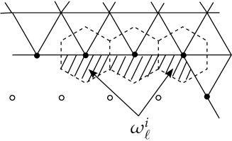
Figure 2. Effective Voronoi cells for the interface nodes (filled circles) are the shaded area in the above figure. ωi<1superscriptsubscript𝜔i1\omega_{\ell}^{\textrm{i}}<1 for the outmost interface atoms which are adjacent to the continuum region.

3.3. Consistency and Optimisation of Reconstruction Parameters

Due to the non-uniqueness of the reconstruction parameters C,ρ,ςsubscript𝐶𝜌𝜍C_{\ell,\rho,\varsigma}, we need to choose the ”optimal” parameters. A naive idea is to use a least-squares approach to minimize C2subscriptnorm𝐶superscript2\|C\|_{\ell^{2}},

minimize Λiρ,ς()|C;ρ,ς|2 subject to (3.3) and (3.6).minimize subscriptsuperscriptΛisubscript𝜌𝜍superscriptsubscript𝐶𝜌𝜍2 subject to (3.3) and (3.6).\text{minimize }\sum_{\ell\in\Lambda^{\textrm{i}}}\sum_{\rho,\varsigma\in\mathcal{R}(\ell)}|C_{\ell;\rho,\varsigma}|^{2}\quad\text{ subject to \eqref{eq:E_pt_grac} and \eqref{eq:F_pt_grac}.} (3.8)

However, the resulting parameters do not give a convergent method.

It is shown in [21, Thm. 6.1] , under the assumptions that d=2𝑑2d=2 and that the atomistic region ΩasuperscriptΩa\Omega^{\textrm{a}} is connected, any a/c coupling scheme of the type (2.4) satisfying the energy and force patch tests (3.2), (3.4) is first-order consistent: if y=yB𝑦superscript𝑦By=y^{\textsf{B}} in ΛΩRΛsubscriptΩ𝑅\Lambda\setminus\Omega_{R} and if y~~𝑦\tilde{y} is an Hloc2subscriptsuperscript𝐻2locH^{2}_{\textrm{loc}}-conforming interpolant of y𝑦y, then

δ(y)δh(Ihy),vhC1h2y~L2(Ω~c)vhL2,𝛿𝑦𝛿superscripthsubscript𝐼𝑦subscript𝑣subscript𝐶1subscriptnormsuperscript2~𝑦superscript𝐿2superscript~Ωcsubscriptnormsubscript𝑣superscript𝐿2\big{\langle}\delta\mathscr{E}(y)-\delta\mathscr{E}^{\textrm{h}}(I_{h}y),v_{h}\big{\rangle}\leq C_{1}\|h\nabla^{2}\tilde{y}\|_{L^{2}(\tilde{\Omega}^{\textrm{c}})}\|\nabla v_{h}\|_{L^{2}}, (3.9)

where C1subscript𝐶1C_{1} is independent of y𝑦y. The dependence of C1subscript𝐶1C_{1} on the reconstruction parameters Csubscript𝐶C_{\ell} is analysed in [29],

C1C1(1+width(Λi))ρ,ς|ρ||ς|Mρ,ς+C1′′subscript𝐶1superscriptsubscript𝐶11widthsuperscriptΛisubscript𝜌𝜍𝜌𝜍subscript𝑀𝜌𝜍superscriptsubscript𝐶1′′\displaystyle C_{1}\leq C_{1}^{\prime}\,(1+\textrm{width}(\Lambda^{\textrm{i}}))\,\sum_{\rho,\varsigma\in\mathcal{R}}|\rho|\,|\varsigma|\,M_{\rho,\varsigma}+C_{1}^{\prime\prime} (3.10)
whereMρ,ς=maxΛiτ,τ()|Vτ,τ(CDy())||C;τ,ρ||C;τ,ς|.wheresubscript𝑀𝜌𝜍subscriptsuperscriptΛisubscript𝜏superscript𝜏subscript𝑉𝜏superscript𝜏subscript𝐶𝐷𝑦subscript𝐶𝜏𝜌subscript𝐶superscript𝜏𝜍\displaystyle\text{where}\quad M_{\rho,\varsigma}=\max_{\ell\in\Lambda^{\textrm{i}}}\sum_{\tau,\tau^{\prime}\in\mathcal{R}(\ell)}|V_{\tau,\tau^{\prime}}(C_{\ell}\cdot Dy(\ell))|\,|C_{\ell;\tau,\rho}|\,|C_{\ell;\tau^{\prime},\varsigma}|.

C1superscriptsubscript𝐶1C_{1}^{\prime} is a generic constant and C1′′superscriptsubscript𝐶1′′C_{1}^{\prime\prime} does not depend on the reconstruction parameters.

Intuitively one may think of

M():=ρ,ς|ρ||ς|τ,τ|Vτ,τ(CDy())||C;τ,ρ||C;τ,ς|assign𝑀subscript𝜌𝜍𝜌𝜍subscript𝜏superscript𝜏subscript𝑉𝜏superscript𝜏subscript𝐶𝐷𝑦subscript𝐶𝜏𝜌subscript𝐶superscript𝜏𝜍M(\ell):=\sum_{\rho,\varsigma}|\rho|\,|\varsigma|\sum_{\tau,\tau^{\prime}}\big{|}V_{\tau,\tau^{\prime}}(C_{\ell}\cdot Dy(\ell))\big{|}\,|C_{\ell;\tau,\rho}|\,|C_{\ell;\tau^{\prime},\varsigma}|

to be a realistic (\ell-dependent) pre-factor. With generic structural assumption |Vτ,τ(CDy())|ω(|τ|)ω(|τ|)less-than-or-similar-tosubscript𝑉𝜏superscript𝜏subscript𝐶𝐷𝑦𝜔𝜏𝜔superscript𝜏|V_{\tau,\tau^{\prime}}(C_{\ell}\cdot Dy(\ell))|\lesssim\omega(|\tau|)\,\omega(|\tau^{\prime}|), where ω𝜔\omega has some decay that is determined by the specific interaction potential, see the discussion for an EAM type potential in App.B.2 [26]. We obtain that

M()𝑀\displaystyle M(\ell) ρ,ς|ρ||ς|τ,τω(|τ|)ω(|τ|)|C;τ,ρ||C;τ,ς|less-than-or-similar-toabsentsubscript𝜌𝜍𝜌𝜍subscript𝜏superscript𝜏𝜔𝜏𝜔superscript𝜏subscript𝐶𝜏𝜌subscript𝐶superscript𝜏𝜍\displaystyle\lesssim\sum_{\rho,\varsigma}|\rho|\,|\varsigma|\sum_{\tau,\tau^{\prime}}\omega(|\tau|)\,\omega(|\tau^{\prime}|)\,|C_{\ell;\tau,\rho}|\,|C_{\ell;\tau^{\prime},\varsigma}|
=(ρ,τ|ρ|ω(|τ|)|C;τ,ρ|)(ς,τ|ς|ω(|τ|)|C;τ,ς|)absentsubscript𝜌𝜏𝜌𝜔𝜏subscript𝐶𝜏𝜌subscript𝜍superscript𝜏𝜍𝜔superscript𝜏subscript𝐶superscript𝜏𝜍\displaystyle=\Big{(}\sum_{\rho,\tau}|\rho|\omega(|\tau|)|C_{\ell;\tau,\rho}|\Big{)}\,\Big{(}\sum_{\varsigma,\tau^{\prime}}|\varsigma|\omega(|\tau^{\prime}|)|C_{\ell;\tau^{\prime},\varsigma}|\Big{)}
=(ρ,τ|ρ|ω(|τ|)|C;τ,ρ|)2.absentsuperscriptsubscript𝜌𝜏𝜌𝜔𝜏subscript𝐶𝜏𝜌2\displaystyle=\Big{(}\sum_{\rho,\tau}|\rho|\omega(|\tau|)|C_{\ell;\tau,\rho}|\Big{)}^{2}.

This indicates that, instead of C2subscriptnorm𝐶superscript2\|C\|_{\ell^{2}}, we should minimize maxΛiρ,τ|ρ|ω(|τ|)|C;τ,ρ|subscriptsuperscriptΛisubscript𝜌𝜏𝜌𝜔𝜏subscript𝐶𝜏𝜌\max_{\ell\in\Lambda^{\textrm{i}}}\sum_{\rho,\tau}|\rho|\omega(|\tau|)|C_{\ell;\tau,\rho}|. Since we do not in general know the generic weights ω𝜔\omega, we simply drop them, and instead minimise ρ,τ|C;τ,ρ|subscript𝜌𝜏subscript𝐶𝜏𝜌\sum_{\rho,\tau}|C_{\ell;\tau,\rho}|. Further, taking the maximum of ΛisuperscriptΛi\ell\in\Lambda^{\textrm{i}} leads to a difficult and computationally expensive multi-objective optimisation problem. Instead, we propose to minimise the 1superscript1\ell^{1}-norm of all the coefficients:

 minimise Λiρ,ς()|C;ρ,ς| subject to (3.3) and (3.6). minimise subscriptsuperscriptΛisubscript𝜌𝜍subscript𝐶𝜌𝜍 subject to (3.3) and (3.6).\text{ minimise }\sum_{\ell\in\Lambda^{\textrm{i}}}\sum_{\rho,\varsigma\in\mathcal{R}(\ell)}|C_{\ell;\rho,\varsigma}|\quad\text{ subject to \eqref{eq:E_pt_grac} and \eqref{eq:F_pt_grac}.} (3.11)

We remark that with the simplifications, the reconstruction parameters only depend on the interaction range, not the particular form of interaction potentials, also, 1superscript1\ell^{1}-minimisation tends to generate “sparse” reconstruction parameters which may present some gain in computational cost in the energy and force assembly routines for E acsuperscript𝐸 acE^{\textrm{ ac}}.

3.4. Stability and stabilisation

The stability of a/c coupling method is of great importance for numerical analysis and the issue of critical stability is essential for practitioners. The issue of stability and (in)stability of a/c coupling scheme is discussed in detail in [22], in particular, a stabilization mechanism is proposed to reduce the stability gap between the a/c coupling methods and the corresponding atomistic model (ground truth). We sketch those results in this subsection.

We expect a/c coupling method has the following stability estimate of the form,

δ2h(Ihy)vh,vhc0vhL22superscript𝛿2superscripthsubscript𝐼𝑦subscript𝑣subscript𝑣subscript𝑐0superscriptsubscriptnormsubscript𝑣superscript𝐿22\langle\delta^{2}\mathscr{E}^{\textrm{h}}(I_{h}y)v_{h},v_{h}\rangle\geq c_{0}\|\nabla v_{h}\|_{L^{2}}^{2} (3.12)

together with consistency and other technical assumptions, we can prove the convergence of the a/c coupling method with inverse function theorem with the form uuhconsistency error/c0less-than-or-similar-tonorm𝑢subscript𝑢consistency errorsubscript𝑐0\|u-u_{h}\|\lesssim\text{consistency error}/c_{0}.

Also, we have the observation that for any uniform deformation, the stability constant of a/c coupling method is less or equal to the stability constant of the corresponding atomistic model. This motivate the introduction of the following stabilization of the interface potential,

Vi(yh):=V(CDyh())+κ|Dnn2yh()|2,assignsuperscriptsubscript𝑉isubscript𝑦𝑉subscript𝐶𝐷subscript𝑦𝜅superscriptsuperscriptsubscript𝐷nn2subscript𝑦2V_{\ell}^{\textrm{i}}(y_{h}):=V\big{(}C_{\ell}\cdot Dy_{h}(\ell)\big{)}+\kappa|D_{\textrm{nn}}^{2}y_{h}(\ell)|^{2}, (3.13)

where κ0𝜅0\kappa\geq 0 is a stabilisation parameter, and |Dnn2yh()|2superscriptsuperscriptsubscript𝐷nn2subscript𝑦2|D_{\textrm{nn}}^{2}y_{h}(\ell)|^{2} is defined as follows: we choose md𝑚𝑑m\geq d linearly independent “nearest-neighbour” directions a1,,amsubscript𝑎1subscript𝑎𝑚a_{1},\dots,a_{m} in the lattice, and denote

|Dnn2yh()|2:=j=1m|yh(+aj)2yh()+yh(aj)|2.assignsuperscriptsuperscriptsubscript𝐷nn2subscript𝑦2superscriptsubscript𝑗1𝑚superscriptsubscript𝑦subscript𝑎𝑗2subscript𝑦subscript𝑦subscript𝑎𝑗2\big{|}D_{\textrm{nn}}^{2}y_{h}(\ell)\big{|}^{2}:=\sum_{j=1}^{m}\big{|}y_{h}(\ell+a_{j})-2y_{h}(\ell)+y_{h}(\ell-a_{j})\big{|}^{2}.

If κ𝜅\kappa is O(1)𝑂1O(1) constant, the stabilization term does not affect consistency, the reconstruction parameters Csubscript𝐶C_{\ell} are still determined by (3.11). However, the stabilisation will affect the computation of the stress tensor in the interface region, which we will introduce in the following section. In [22], we have theoretically proved for some symmetric configuration and numerical justified for prototypical examples that such stabilization can reduce the stability gap and suppress spurious critical mode for the a/c coupling methods.

4. Stress formulation

The stress formulation plays a significant role in the analysis of a/c coupling methods. Given deformation yyB𝒰1,2𝑦superscript𝑦𝐵superscript𝒰12y-y^{B}\in\mathscr{U}^{1,2} and an energy functional (y)𝑦\mathscr{E}(y), the first Piola-Kirchhoff stress σ(y)𝜎𝑦\sigma(y) satisfies

δ(y),v=dσ(y):vdx,:𝛿𝑦𝑣subscriptsuperscript𝑑𝜎𝑦𝑣d𝑥\langle\delta\mathscr{E}(y),v\rangle=\int_{\mathbb{R}^{d}}\sigma(y):\nabla v\,{\textrm{d}}x,

for any v𝒰1,2𝑣superscript𝒰12v\in\mathscr{U}^{1,2}.

From the first variation of the a/c energy functional (3.5) and (3.7), we expect to derive its stress formulation, namely, for any vh𝒰hsubscript𝑣subscript𝒰v_{h}\in\mathscr{U}_{h},

δh(yh),vh=𝛿superscripthsubscript𝑦subscript𝑣absent\displaystyle\langle\delta\mathscr{E}^{\textrm{h}}(y_{h}),v_{h}\rangle= δa,vh+δi,vh+δc,vh𝛿superscriptasubscript𝑣𝛿superscriptisubscript𝑣𝛿superscriptcsubscript𝑣\displaystyle\langle\delta\mathscr{E}^{\textrm{a}},v_{h}\rangle+\langle\delta\mathscr{E}^{\textrm{i}},v_{h}\rangle+\langle\delta\mathscr{E}^{\textrm{c}},v_{h}\rangle
=\displaystyle= Ωaσa:vhdx+Ωiσi:vhdx+Ωcσc:Tvh:subscriptsuperscriptΩasuperscript𝜎asubscript𝑣d𝑥subscriptsuperscriptΩisuperscript𝜎i:subscript𝑣d𝑥subscriptsuperscriptΩcsuperscript𝜎c:subscript𝑇subscript𝑣\displaystyle\int_{\Omega^{\textrm{a}}}\sigma^{\textrm{a}}:\nabla v_{h}\,{\textrm{d}}x+\int_{\Omega^{\textrm{i}}}\sigma^{\textrm{i}}:\nabla v_{h}\,{\textrm{d}}x+\int_{\Omega^{\textrm{c}}}\sigma^{\textrm{c}}:\nabla_{T}v_{h}
=\displaystyle= Ωσh:vhdx:subscriptΩsuperscript𝜎hsubscript𝑣d𝑥\displaystyle\int_{\Omega}\sigma^{\textrm{h}}:\nabla v_{h}\,{\textrm{d}}x

In this section, we first review the stress tensor formula derived by [26] in § 4.1 which is essential for the a priori analysis, however, this formula is not suitable for the a posteriori estimate. In § 4.2 we introduce a novel computable stress tensor expression, which is convenient for the purpose of a posterior error estimation and adaptive algorithm. We discuss the assembly of stress tensor for our model problem in § 7.1.

4.1. Stress Tensor Formulation in [26]

We first discuss the formula for σasuperscript𝜎a\sigma^{\textrm{a}}. For simplicity, consider full atomistic energy \mathscr{E} in (2.2). The ”canonical weak form” of δ𝛿\delta\mathscr{E} is

δ(u),v=ΛρV,ρ(u)Dρv(),for v𝒰1,2formulae-sequence𝛿𝑢𝑣subscriptΛsubscript𝜌subscript𝑉𝜌𝑢subscript𝐷𝜌𝑣for 𝑣superscript𝒰12\langle\delta\mathscr{E}(u),v\rangle=\sum_{\ell\in\Lambda}\sum_{\rho\in\mathcal{R}}V_{\ell,\rho}(u)\cdot D_{\rho}v(\ell),\quad\text{for }v\in\mathscr{U}^{1,2} (4.1)

Now we define a modified version of the canonical weak form. Let

v:=ζ¯v¯.assignsuperscript𝑣¯𝜁¯𝑣v^{\ast}:=\bar{\zeta}\ast\bar{v}. (4.2)

The finite differences Dρv(ζ)subscript𝐷𝜌superscript𝑣𝜁D_{\rho}v^{\ast}(\zeta) can be expressed as in [34],

Dρv()=subscript𝐷𝜌superscript𝑣absent\displaystyle D_{\rho}v^{\ast}(\ell)= s=01ρv(+sρ)ds=ds=01ζ¯(+sρx)ρv¯(x)dsdxsuperscriptsubscript𝑠01subscript𝜌superscript𝑣𝑠𝜌d𝑠subscriptsuperscript𝑑superscriptsubscript𝑠01¯𝜁𝑠𝜌𝑥subscript𝜌¯𝑣𝑥d𝑠d𝑥\displaystyle\int_{s=0}^{1}\nabla_{\rho}v^{\ast}(\ell+s\rho)\,{\textrm{d}}s=\int_{\mathbb{R}^{d}}\int_{s=0}^{1}\bar{\zeta}(\ell+s\rho-x)\nabla_{\rho}\bar{v}(x)\,{\textrm{d}}s\,{\textrm{d}}x
=\displaystyle= dχ,ρ(x)ρv¯(x)dxsubscriptsuperscript𝑑subscript𝜒𝜌𝑥subscript𝜌¯𝑣𝑥d𝑥\displaystyle\int_{\mathbb{R}^{d}}\chi_{\ell,\rho}(x)\nabla_{\rho}\bar{v}(x)\,{\textrm{d}}x (4.3)

where χ,ρsubscript𝜒𝜌\chi_{\ell,\rho} is a generic weighting function defined as below, can be understood as a mollified version of the line measure.

χ,ρ(x):=01ζ¯(+tρx)dtassignsubscript𝜒𝜌𝑥superscriptsubscript01¯𝜁𝑡𝜌𝑥d𝑡\chi_{\ell,\rho}(x):=\int_{0}^{1}\bar{\zeta}(\ell+t\rho-x)\,{\textrm{d}}t (4.4)

Now, we replace the test function in (4.1) from v𝑣v to vsuperscript𝑣v^{\ast},

δ(y),v=𝛿𝑦superscript𝑣absent\displaystyle\langle\delta\mathscr{E}(y),v^{\ast}\rangle= ΛaρρVdχ,ρ(x)ρv¯(x)dxsubscriptsuperscriptΛ𝑎subscript𝜌subscript𝜌subscript𝑉subscriptsuperscript𝑑subscript𝜒𝜌𝑥subscript𝜌¯𝑣𝑥d𝑥\displaystyle\sum_{\ell\in\Lambda^{a}}\sum_{\rho\in\mathcal{R}}\partial_{\rho}V_{\ell}\cdot\int_{\mathbb{R}^{d}}\chi_{\ell,\rho}(x)\nabla_{\rho}\bar{v}(x)\,{\textrm{d}}x
=\displaystyle= d{Λaρ[ρVρ]χ,ρ(x)}:v¯dx:subscriptsuperscript𝑑subscriptsuperscriptΛ𝑎subscript𝜌delimited-[]subscript𝜌tensor-productsubscript𝑉𝜌subscript𝜒𝜌𝑥¯𝑣d𝑥\displaystyle\int_{\mathbb{R}^{d}}\left\{\sum_{\ell\in\Lambda^{a}}\sum_{\rho\in\mathcal{R}}\left[\partial_{\rho}V_{\ell}\otimes\rho\right]\chi_{\ell,\rho}(x)\right\}:\nabla\bar{v}\,{\textrm{d}}x

Thus, we have shown that for yyB𝒰1,2𝑦superscript𝑦Bsuperscript𝒰12y-y^{\textsf{B}}\in\mathscr{U}^{1,2} and v𝒰𝑣𝒰v\in\mathscr{U} with compact support ,

δ(y),v=dσa(y;x):v¯dx,:𝛿𝑦superscript𝑣subscriptsuperscript𝑑superscript𝜎a𝑦𝑥¯𝑣d𝑥\langle\delta\mathscr{E}(y),v^{\ast}\rangle=\int_{\mathbb{R}^{d}}\sigma^{\textrm{a}}(y;x):\nabla\bar{v}\,{\textrm{d}}x,

with

σa(y;x):=Λaρ[ρVρ]χ,ρ(x),assignsuperscript𝜎a𝑦𝑥subscriptsuperscriptΛasubscript𝜌delimited-[]subscript𝜌tensor-productsubscript𝑉𝜌subscript𝜒𝜌𝑥\sigma^{\textrm{a}}(y;x):=\sum_{\ell\in\Lambda^{\textrm{a}}}\sum_{\rho\in\mathcal{R}}\left[\partial_{\rho}V_{\ell}\otimes\rho\right]\chi_{\ell,\rho}(x), (4.5)

Through an analogy to the analysis above, δi(y),v𝛿superscripti𝑦superscript𝑣\langle\delta\mathscr{E}^{\textrm{i}}(y),v^{\ast}\rangle could be written as,

δi(y),v=dσi(y;x):v¯dx,:𝛿superscripti𝑦superscript𝑣subscriptsuperscript𝑑superscript𝜎i𝑦𝑥¯𝑣d𝑥\langle\delta\mathscr{E}^{\textrm{i}}(y),v^{\ast}\rangle=\int_{\mathbb{R}^{d}}\sigma^{\textrm{i}}(y;x):\nabla\bar{v}\,{\textrm{d}}x,

where

σi(y;x):=Λiρ[ωiρViρ]χ,ρ(x),assignsuperscript𝜎i𝑦𝑥subscriptsuperscriptΛisubscript𝜌delimited-[]subscriptsuperscript𝜔isubscript𝜌tensor-productsubscriptsuperscript𝑉i𝜌subscript𝜒𝜌𝑥\sigma^{\textrm{i}}(y;x):=\sum_{\ell\in\Lambda^{\textrm{i}}}\sum_{\rho\in\mathcal{R}}\left[\omega^{\textrm{i}}_{\ell}\partial_{\rho}V^{\textrm{i}}_{\ell}\otimes\rho\right]\chi_{\ell,\rho}(x), (4.6)

Finally, the first Piola-Kirchhoff stress of the Cauchy-Born model gives,

σc(y;x)=W(y(x))superscript𝜎c𝑦𝑥𝑊𝑦𝑥\sigma^{\textrm{c}}(y;x)=\partial W(\nabla y(x)) (4.7)

By proper regularity assumptions on V𝑉V and y𝑦y, it can be shown that σc(y;x)superscript𝜎c𝑦𝑥\sigma^{\textrm{c}}(y;x) is second order consistent to σa(y;x)superscript𝜎a𝑦𝑥\sigma^{\textrm{a}}(y;x).

The stress tensor expression introduced in this section is important for the a priori analysis of Caucy-Born continuum model in [26] and blended a/c coupling method [12]. However, since σa(y;x)superscript𝜎a𝑦𝑥\sigma^{\textrm{a}}(y;x) and σi(y;x)superscript𝜎i𝑦𝑥\sigma^{\textrm{i}}(y;x) depend on x𝑥x through χ,ρ(x)subscript𝜒𝜌𝑥\chi_{\ell,\rho}(x), it is relatively difficult to calculate the value of them, which is crucial for the a posteriori error estimates and adaptive algorithm. In the next section, we will introduce a computable expression of stress tensor.

4.2. A Computable Stress Tensor Formulation

For the nearest neighbour interactions [40], we use the canonical expressions of δ𝛿\delta\mathscr{E} (δh𝛿superscripth\delta\mathscr{E}^{\textrm{h}}) to define σasuperscript𝜎a\sigma^{\textrm{a}} (σhsuperscript𝜎h\sigma^{\textrm{h}}). In that case, σasuperscript𝜎a\sigma^{\textrm{a}} (σhsuperscript𝜎h\sigma^{\textrm{h}}) is piecewise constant over the triangulation 𝒯asubscript𝒯a\mathcal{T}_{\textrm{a}} (𝒯hsubscript𝒯h\mathcal{T}_{\textrm{h}}). In this section, we will extend this formulation to general finite range interactions.

Consider the canonical weak form of δ𝛿\delta\mathscr{E} in (4.1), instead of replacing v𝑣v with vsuperscript𝑣v^{\ast}, we distribute Dρvsubscript𝐷𝜌𝑣D_{\rho}v to relevant triangles in order to transfer the sum with respect to atoms to the sum over elements in the micro-triangulation 𝒯asubscript𝒯a\mathcal{T}_{\textrm{a}} induced by the reference lattice ΛΛ\Lambda. We express Dρvsubscript𝐷𝜌𝑣D_{\rho}v as,

Dρv()=T𝒯ρωρ(T)Tvρsubscript𝐷𝜌𝑣subscript𝑇superscriptsubscript𝒯𝜌superscriptsubscript𝜔𝜌𝑇subscript𝑇𝑣𝜌D_{\rho}v(\ell)=\sum_{T\in\mathcal{T}_{\ell}^{\rho}}\omega_{\ell}^{\rho}(T)\nabla_{T}v\cdot\rho (4.8)

where 𝒯ρ:={T𝒯a|length(T(,+ρ))>0}assignsuperscriptsubscript𝒯𝜌conditional-set𝑇subscript𝒯alength𝑇𝜌0\mathcal{T}_{\ell}^{\rho}:=\{T\in\mathcal{T}_{\textrm{a}}|\textrm{length}(T\cap(\ell,\ell+\rho))>0\} is the set which contains the elements that form the compact support of bond (,+ρ)𝜌(\ell,\ell+\rho), ωρ(T)superscriptsubscript𝜔𝜌𝑇\omega_{\ell}^{\rho}(T) is an appropriate weight function. The implementation details for two dimensional triangular lattice will be discussed in detail in § 7.1.

For any yyB𝒰1,2,v𝒰1,2formulae-sequence𝑦superscript𝑦Bsuperscript𝒰12𝑣superscript𝒰12y-y^{\textsf{B}}\in\mathscr{U}^{1,2},v\in\mathscr{U}^{1,2},

δ(y),v=ΛρρVDρv=ΛρρV(ωρ(b=(,+ρ)TTv)ρ)=Λρ2|T|detAρVρ:(ωρb=(,+ρ)TTv)=|T|T𝒯aρ1detAb=(,+ρ)T2ωρρVρ:(Tv),v𝒰:𝛿𝑦𝑣subscriptΛsubscript𝜌subscriptsubscript𝜌subscript𝑉subscript𝐷𝜌𝑣subscriptΛsubscript𝜌subscriptsubscript𝜌subscript𝑉subscript𝜔𝜌subscript𝑏𝜌𝑇subscript𝑇𝑣𝜌subscriptΛsubscript𝜌subscript2𝑇Asubscript𝜌tensor-productsubscript𝑉𝜌subscript𝜔𝜌subscript𝑏𝜌𝑇subscript𝑇𝑣𝑇subscript𝑇subscript𝒯asubscript𝜌subscript1Asubscript𝑏𝜌𝑇2subscript𝜔𝜌subscript𝜌tensor-productsubscript𝑉𝜌:subscript𝑇𝑣for-all𝑣𝒰\begin{split}\langle\delta\mathscr{E}(y),v\rangle&=\sum_{\ell\in\Lambda}\sum_{\rho\in\mathcal{R}_{\ell}}\partial_{\rho}V_{\ell}\cdot D_{\rho}v\\ &=\sum_{\ell\in\Lambda}\sum_{\rho\in\mathcal{R}_{\ell}}\partial_{\rho}V_{\ell}\cdot\left(\omega_{\rho}\left(\sum_{b=(\ell,\ell+\rho)\cap T\neq\emptyset}\nabla_{T}v\right)\cdot\rho\right)\\ &=\sum_{\ell\in\Lambda}\sum_{\rho\in\mathcal{R}_{\ell}}\frac{2|T|}{\det{\textsf{A}}}\partial_{\rho}V_{\ell}\otimes\rho:\left(\omega_{\rho}\sum_{b=(\ell,\ell+\rho)\cap T\neq\emptyset}\nabla_{T}v\right)\\ &=|T|\sum_{T\in\mathcal{T}_{\textrm{a}}}\sum_{\rho\in\mathcal{R}_{\ell}}\frac{1}{\det{\textsf{A}}}\sum_{b=(\ell,\ell+\rho)\cap T\neq\emptyset}2\omega_{\rho}\partial_{\rho}V_{\ell}\otimes\rho:\left(\nabla_{T}v\right),\forall v\in\mathscr{U}\end{split} (4.9)

ωρ(T)superscriptsubscript𝜔𝜌𝑇\omega_{\ell}^{\rho}(T) represents the contribution of the value of ρV(Tyh)ρsubscript𝜌tensor-product𝑉subscript𝑇subscript𝑦𝜌\partial_{\rho}V(\nabla_{T}y_{h})\otimes\rho from element T𝑇T, which depends on the specific type of ρ𝜌\rho\in\mathcal{R}.

Recall from (2.4) and (3.1), the GRAC a/c coupling energy functional is of the form

h(yh):=ΛaV(yh)+ΛiωVi(yh)+T𝒯hωTW(yh|T)assignsuperscripthsubscript𝑦subscriptsuperscriptΛasubscript𝑉subscript𝑦subscriptsuperscriptΛisubscript𝜔subscriptsuperscript𝑉isubscript𝑦subscript𝑇subscript𝒯hsubscript𝜔𝑇𝑊evaluated-atsubscript𝑦𝑇\mathscr{E}^{\textrm{h}}(y_{h}):=\sum_{\ell\in\Lambda^{\textrm{a}}}V_{\ell}(y_{h})+\sum_{\ell\in\Lambda^{\textrm{i}}}\omega_{\ell}V^{\textrm{i}}_{\ell}(y_{h})+\sum_{T\in\mathcal{T}_{\textrm{h}}}\omega_{T}W(\nabla y_{h}|_{T})

with

Vi(y):=V((ςC;ρ,ςDςy())ρ)assignsuperscriptsubscript𝑉i𝑦subscript𝑉subscriptsubscript𝜍subscriptsubscript𝐶𝜌𝜍subscript𝐷𝜍𝑦𝜌subscriptV_{\ell}^{\textrm{i}}(y):=V_{\ell}\Big{(}\big{(}{\sum_{\varsigma\in\mathcal{R}_{\ell}}C_{\ell;\rho,\varsigma}D_{\varsigma}y(\ell)}\big{)}_{\rho\in\mathcal{R}_{\ell}}\Big{)}

With the decomposition of the first variation of GRAC in (3.5), the first variation of the interface energy isuperscripti\mathscr{E}^{\textrm{i}} has the following form,

δΛiωVi(yh),vh=δΛiωV((ςC;ρ,ςDςyh)ρ),vh=ΛiωρρV(ςC;ρ,ςDςvh())=ΛiωρςρVC;ρ,ς(ως(b=(,+ς)TTvh)ς)=Λi2ω|T|detAς(ρC;ρ,ςρVς):(ωςb=(,+ς)TTvh)=T𝒯hi|T|detAςb=(,+ς)T2ω(ρC;ρ,ςωςρVς):(Tvh):𝛿subscriptsuperscriptΛisubscript𝜔subscriptsuperscript𝑉isubscript𝑦subscript𝑣𝛿subscriptsuperscriptΛisubscript𝜔subscript𝑉subscriptsubscript𝜍subscriptsubscript𝐶𝜌𝜍subscript𝐷𝜍subscript𝑦𝜌subscriptsubscript𝑣subscriptsuperscriptΛisubscript𝜔subscript𝜌subscriptsubscript𝜌subscript𝑉subscript𝜍subscriptsubscript𝐶𝜌𝜍subscript𝐷𝜍subscript𝑣subscriptsuperscriptΛisubscript𝜔subscript𝜌subscriptsubscript𝜍subscriptsubscript𝜌subscript𝑉subscript𝐶𝜌𝜍subscript𝜔𝜍subscript𝑏𝜍𝑇subscript𝑇subscript𝑣𝜍subscriptsuperscriptΛi2subscript𝜔𝑇Asubscript𝜍subscriptsubscript𝜌subscriptsubscript𝐶𝜌𝜍subscript𝜌tensor-productsubscript𝑉𝜍subscript𝜔𝜍subscript𝑏𝜍𝑇subscript𝑇subscript𝑣subscript𝑇superscriptsubscript𝒯hi𝑇Asubscript𝜍subscriptsubscript𝑏𝜍𝑇2subscript𝜔subscript𝜌subscriptsubscript𝐶𝜌𝜍subscript𝜔𝜍subscript𝜌tensor-productsubscript𝑉𝜍:subscript𝑇subscript𝑣\begin{split}\langle\delta\sum_{\ell\in\Lambda^{\textrm{i}}}\omega_{\ell}V^{\textrm{i}}_{\ell}(y_{h}),v_{h}\rangle&=\langle\delta\sum_{\ell\in\Lambda^{\textrm{i}}}\omega_{\ell}V_{\ell}\Big{(}\big{(}{\sum_{\varsigma\in\mathcal{R}_{\ell}}C_{\ell;\rho,\varsigma}D_{\varsigma}y_{h}}\big{)}_{\rho\in\mathcal{R}_{\ell}}\Big{)},v_{h}\rangle\\ &=\sum_{\ell\in\Lambda^{\textrm{i}}}\omega_{\ell}\sum_{\rho\in\mathcal{R}_{\ell}}\partial_{\rho}V_{\ell}\cdot\left(\sum_{\varsigma\in\mathcal{R}_{\ell}}C_{\ell;\rho,\varsigma}D_{\varsigma}v_{h}(\ell)\right)\\ &=\sum_{\ell\in\Lambda^{\textrm{i}}}\omega_{\ell}\sum_{\rho\in\mathcal{R}_{\ell}}\sum_{\varsigma\in\mathcal{R}_{\ell}}\partial_{\rho}V_{\ell}C_{\ell;\rho,\varsigma}\cdot\left(\omega_{\varsigma}\left(\sum_{b=(\ell,\ell+\varsigma)\cap T\neq\emptyset}\nabla_{T}v_{h}\right)\cdot\varsigma\right)\\ &=\sum_{\ell\in\Lambda^{\textrm{i}}}\frac{2\omega_{\ell}|T|}{\det{\textsf{A}}}\sum_{\varsigma\in\mathcal{R}_{\ell}}\left(\sum_{\rho\in\mathcal{R}_{\ell}}C_{\ell;\rho,\varsigma}\partial_{\rho}V_{\ell}\otimes\varsigma\right):\left(\omega_{\varsigma}\sum_{b=(\ell,\ell+\varsigma)\cap T\neq\emptyset}\nabla_{T}v_{h}\right)\\ &=\sum_{T\in\mathcal{T}_{\textrm{h}}^{\textrm{i}}}\frac{|T|}{\det{\textsf{A}}}\sum_{\varsigma\in\mathcal{R}_{\ell}}\sum_{b=(\ell,\ell+\varsigma)\cap T\neq\emptyset}2\omega_{\ell}\left(\sum_{\rho\in\mathcal{R}_{\ell}}C_{\ell;\rho,\varsigma}\omega_{\varsigma}\partial_{\rho}V_{\ell}\otimes\varsigma\right):\left(\nabla_{T}v_{h}\right)\end{split} (4.10)

Consider the continuum model, for any yhyB𝒰h,vh𝒰hformulae-sequencesubscript𝑦superscript𝑦Bsubscript𝒰subscript𝑣subscript𝒰y_{h}-y^{\textsf{B}}\in\mathscr{U}_{h},v_{h}\in\mathscr{U}_{h}, we have

δc(yh),vh𝛿superscriptcsubscript𝑦subscript𝑣\displaystyle\langle\delta\mathscr{E}^{\textrm{c}}(y_{h}),v_{h}\rangle =T𝒯h|T|W(Tyh)absentsubscript𝑇subscript𝒯h𝑇𝑊subscript𝑇subscript𝑦\displaystyle=\sum_{T\in\mathcal{T}_{\textrm{h}}}|T|\partial W(\nabla_{T}y_{h}) (4.11)
=T𝒯h|T|ρρV(Tyh)ρ:Tvh,:absentsubscript𝑇subscript𝒯h𝑇subscript𝜌subscript𝜌tensor-product𝑉subscript𝑇subscript𝑦𝜌subscript𝑇subscript𝑣\displaystyle=\sum_{T\in\mathcal{T}_{\textrm{h}}}|T|\sum_{\rho\in\mathcal{R}}\partial_{\rho}V(\nabla_{T}y_{h})\otimes\rho:\nabla_{T}v_{h}, (4.12)

Adding the stabilization term as in (3.13), we are ready to obtain the first variation of the (stabilized) GRAC coupling method,

δh(yh),vh𝛿superscripthsubscript𝑦subscript𝑣\displaystyle\langle\delta\mathscr{E}^{\textrm{h}}(y_{h}),v_{h}\rangle =T𝒯ha𝒯hi|T|detAρb=(,+ρ)T2ωωρ(T)ρVhρ:(Tvh):absentsubscript𝑇superscriptsubscript𝒯hasuperscriptsubscript𝒯hi𝑇Asubscript𝜌subscriptsubscript𝑏𝜌𝑇2subscript𝜔superscriptsubscript𝜔𝜌𝑇subscript𝜌tensor-productsuperscriptsubscript𝑉𝜌subscript𝑇subscript𝑣\displaystyle=\sum_{T\in\mathcal{T}_{\textrm{h}}^{\textrm{a}}\cup\mathcal{T}_{\textrm{h}}^{\textrm{i}}}\frac{|T|}{\det{\textsf{A}}}\sum_{\rho\in\mathcal{R}_{\ell}}\sum_{b=(\ell,\ell+\rho)\cap T\neq\emptyset}2\omega_{\ell}\omega_{\ell}^{\rho}(T)\partial_{\rho}V_{\ell}^{h}\otimes\rho:\left(\nabla_{T}v_{h}\right)
+T𝒯hωTdetAρρV(Tyh)ρ:Tvh,:subscript𝑇subscript𝒯hsubscript𝜔𝑇Asubscript𝜌subscript𝜌tensor-product𝑉subscript𝑇subscript𝑦𝜌subscript𝑇subscript𝑣\displaystyle+\sum_{T\in\mathcal{T}_{\textrm{h}}}\frac{\omega_{T}}{\det{\textsf{A}}}\sum_{\rho\in\mathcal{R}}\partial_{\rho}V(\nabla_{T}y_{h})\otimes\rho:\nabla_{T}v_{h}, (4.13)
+CstabT𝒯hiζnnb=(,+ζ)T2ωζ(T)dnn3(,ζ)ζ:T:subscript𝐶stabsubscriptsuperscript𝑇superscriptsubscript𝒯h𝑖subscript𝜁subscriptnnsubscriptsuperscript𝑏𝜁superscript𝑇tensor-product2superscriptsubscript𝜔𝜁𝑇superscriptsubscriptdnn3𝜁𝜁subscriptsuperscript𝑇\displaystyle+C_{\textrm{stab}}\sum_{T^{\prime}\in\mathcal{T}_{\textrm{h}}^{i}}\sum_{\zeta\in\mathbb{R}_{\textrm{nn}}}\sum_{b^{\prime}=(\ell,\ell+\zeta)\cap T^{\prime}\neq\emptyset}2\omega_{\ell}^{\zeta}(T)\textrm{d}_{\textrm{nn}}^{3}(\ell,\zeta)\otimes\zeta:\nabla_{T^{\prime}}
whereρVh:={ρV,ΛaςC;ς,ρςV,Λiassignwheresubscript𝜌superscriptsubscript𝑉casessubscript𝜌subscript𝑉superscriptΛ𝑎missing-subexpressionsubscript𝜍subscriptsubscript𝐶𝜍𝜌subscript𝜍subscript𝑉superscriptΛ𝑖missing-subexpression\text{where}\quad\partial_{\rho}V_{\ell}^{h}:=\left\{\begin{array}[]{rl}\partial_{\rho}V_{\ell},\quad\ell\in\Lambda^{a}&\\ \sum_{\varsigma\in\mathcal{R}_{\ell}}C_{\ell;\varsigma,\rho}\partial_{\varsigma}V_{\ell},\quad\ell\in\Lambda^{i}&\end{array}\right.

and

dnn3(,ζ)=yh(+2ζ)+3yh(+ζ)3yh()+yh(ζ)superscriptsubscriptdnn3𝜁subscript𝑦2𝜁3subscript𝑦𝜁3subscript𝑦subscript𝑦𝜁\textrm{d}_{\textrm{nn}}^{3}(\ell,\zeta)=-y_{h}(\ell+2\zeta)+3y_{h}(\ell+\zeta)-3y_{h}(\ell)+y_{h}(\ell-\zeta)

Cstabsubscript𝐶stabC_{\textrm{stab}} is a constant equal to 1 if stabilisation is applied, and 0 otherwise.

We can define the atomistic stress tensor σasuperscript𝜎a\sigma^{\textrm{a}} (with respect to micro-triangulation 𝒯asubscript𝒯a\mathcal{T}_{\textrm{a}}), the continuum stress tensor σcsuperscript𝜎c\sigma^{\textrm{c}}, and the a/c stress tensor σhsuperscript𝜎h\sigma^{\textrm{h}} by the following first variations of different models,

δa(y),v𝛿superscripta𝑦𝑣\displaystyle\langle\delta\mathscr{E}^{\textrm{a}}(y),v\rangle =T𝒯a|T|σa(y;T):Tv,v𝒰,:absentsubscript𝑇subscript𝒯a𝑇superscript𝜎a𝑦𝑇subscript𝑇𝑣for-all𝑣𝒰\displaystyle=\sum_{T\in\mathcal{T}_{\textrm{a}}}|T|\sigma^{\textrm{a}}(y;T):\nabla_{T}v,\forall v\in\mathscr{U}, (4.14)
δc(yh),vh𝛿superscriptcsubscript𝑦subscript𝑣\displaystyle\langle\delta\mathscr{E}^{\textrm{c}}(y_{h}),v_{h}\rangle =T𝒯h|T|σc(yh;T):Tvh,vh𝒰h,:absentsubscript𝑇subscript𝒯h𝑇superscript𝜎csubscript𝑦𝑇subscript𝑇subscript𝑣for-allsubscript𝑣subscript𝒰\displaystyle=\sum_{T\in\mathcal{T}_{\textrm{h}}}|T|\sigma^{\textrm{c}}(y_{h};T):\nabla_{T}v_{h},\forall v_{h}\in\mathscr{U}_{h}, (4.15)
δh(yh),vh𝛿superscripthsubscript𝑦subscript𝑣\displaystyle\langle\delta\mathscr{E}^{\textrm{h}}(y_{h}),v_{h}\rangle =T𝒯h|T|σh(yh;T):Tvh,vh𝒰h.:absentsubscript𝑇subscript𝒯h𝑇superscript𝜎hsubscript𝑦𝑇subscript𝑇subscript𝑣for-allsubscript𝑣subscript𝒰\displaystyle=\sum_{T\in\mathcal{T}_{\textrm{h}}}|T|\sigma^{\textrm{h}}(y_{h};T):\nabla_{T}v_{h},\forall v_{h}\in\mathscr{U}_{h}. (4.16)

From the above discussions, we have the following ”canonical” choices for σasuperscript𝜎a\sigma^{\textrm{a}}, σcsuperscript𝜎c\sigma^{\textrm{c}} and σhsuperscript𝜎h\sigma^{\textrm{h}}.

σa(y;T):=assignsuperscript𝜎a𝑦𝑇absent\displaystyle\sigma^{\textrm{a}}(y;T):=~{} 1detAρb=(,+ρ)T2ωρ(T)ρVρ,1Asubscript𝜌subscriptsubscript𝑏𝜌𝑇2superscriptsubscript𝜔𝜌𝑇subscript𝜌tensor-productsubscript𝑉𝜌\displaystyle\frac{1}{\det{\textsf{A}}}\sum_{\rho\in\mathcal{R}_{\ell}}\sum_{b=(\ell,\ell+\rho)\cap T\neq\emptyset}2\omega_{\ell}^{\rho}(T)\partial_{\rho}V_{\ell}\otimes\rho, (4.17)
σc(yh;T):=assignsuperscript𝜎csubscript𝑦𝑇absent\displaystyle\sigma^{\textrm{c}}(y_{h};T):=~{} 1detAρρV(Tyh)ρ,1Asubscript𝜌subscript𝜌tensor-product𝑉subscript𝑇subscript𝑦𝜌\displaystyle\frac{1}{\det{\textsf{A}}}\sum_{\rho\in\mathcal{R}}\partial_{\rho}V(\nabla_{T}y_{h})\otimes\rho, (4.18)
σh(yh;T):=assignsuperscript𝜎hsubscript𝑦𝑇absent\displaystyle\sigma^{\textrm{h}}(y_{h};T):=~{} 1detA(ρb=(,+ρ)T2ωωρ(T)ρVhρ+ωT|T|σc(yh;T)\displaystyle\frac{1}{\det{\textsf{A}}}\left(\sum_{\rho\in\mathcal{R}_{\ell}}\sum_{b=(\ell,\ell+\rho)\cap T\neq\emptyset}2\omega_{\ell}\omega_{\ell}^{\rho}(T)\partial_{\rho}V_{\ell}^{h}\otimes\rho+\frac{\omega_{T}}{|T|}\sigma^{\textrm{c}}(y_{h};T)\right. (4.19)
+Cstabζnnb=(,+ζ)TT𝒯i2ωζ(T)dnn3(,ζ)ζ).\displaystyle\left.+C_{\textrm{stab}}\sum_{\zeta\in\mathbb{R}_{\textrm{nn}}}\sum_{\begin{subarray}{c}b^{\prime}=(\ell,\ell+\zeta)\cap T^{\prime}\neq\emptyset\\ T^{\prime}\in\mathcal{T}^{\textrm{i}}\end{subarray}}2\omega_{\ell}^{\zeta}(T)\textrm{d}_{\textrm{nn}}^{3}(\ell,\zeta)\otimes\zeta\right).

However, the stress tensors defined through (4.14)-(4.16) are not unique due to the following results.


Definition 1. We call piecewise constant tensor field σP0(𝒯)2×2𝜎subscriptP0superscript𝒯22\sigma\in\textrm{P}_{0}(\mathcal{T})^{2\times 2} divergence free if

T𝒯|T|σ(T):Tv0,v(P1(𝒯))2.:subscript𝑇𝒯𝑇𝜎𝑇formulae-sequencesubscript𝑇𝑣0for-all𝑣superscriptsubscriptP1𝒯2\sum_{T\in\mathcal{T}}|T|\sigma(T):\nabla_{T}v\equiv 0,\forall v\in({\textrm{P}}_{1}(\mathcal{T}))^{2}.

Corollary 4.1. By definitions (4.16), it is easy to know that the force patch test condition (3.4) is equivalent to that σh(yF)superscript𝜎hsubscript𝑦F\sigma^{\textrm{h}}(y_{\textsf{F}}) is divergence free for any constant deformation gradient F.

The discrete divergence free tensor fields over the triangulation 𝒯𝒯\mathcal{T} can be characterized by the non-conforming Crouzeix-Raviart finite elements [28, 21]. The Crouzeix-Raviart finite element space over 𝒯𝒯\mathcal{T} is defined as

N1(𝒯)={c:T𝒯int(T)|\displaystyle N_{1}(\mathcal{T})=\{c:\bigcup_{T\in\mathcal{T}}\textrm{int}(T)\to\mathbb{R}\quad\big{|} c is piecewise affine w.r.t. 𝒯,and𝑐 is piecewise affine w.r.t. 𝒯and\displaystyle\quad c\textrm{ is piecewise affine w.r.t. }\mathcal{T},\textrm{and}
continuous in edge midpoints qf,f}\displaystyle\textrm{continuous in edge midpoints }q_{f},\forall f\in\mathcal{F}\}

The following lemma in [28] characterizes the discrete divergence-free tensor field.


Lemma 4.2. A tensor field σP0(𝒯)2×2𝜎subscriptP0superscript𝒯22\sigma\in\textsf{P}_{0}(\mathcal{T})^{2\times 2} is divergence free if and only if there exists a constant σ02×2subscript𝜎0superscript22\sigma_{0}\in\mathbb{R}^{2\times 2} and a function cN1(𝒯)2𝑐subscript𝑁1superscript𝒯2c\in N_{1}(\mathcal{T})^{2} such that

σ=σ0+cJ,whereJ=[0110]SO(2).formulae-sequence𝜎subscript𝜎0𝑐JwhereJdelimited-[]matrix0110SO2\sigma=\sigma_{0}+\nabla c\textsf{J},\qquad\textrm{where}\quad\textsf{J}=\left[\begin{matrix}0&-1\\ 1&0\end{matrix}\right]\in{\textsf{SO}}(2).

The following corollary provides a representation of the stress tensors defined in (4.14)-(4.16).


Corollary 4.3. The stress tensors in the definitions (4.14)-(4.16) are not unique. Given any stress tensor σP0(𝒯)2×2𝜎subscriptP0superscript𝒯22\sigma\in\textsf{P}_{0}(\mathcal{T})^{2\times 2} satisfies one of the definitions (4.14)-(4.16) , where 𝒯𝒯\mathcal{T} is the corresponding triangulation. Define the admissible set as Adm(σ):={σ+cJ,cN1(𝒯)2}assignAdm𝜎𝜎𝑐J𝑐subscript𝑁1superscript𝒯2\textrm{Adm}(\sigma):=\{\sigma+\nabla c\textsf{J},c\in N_{1}(\mathcal{T})^{2}\}, then any σAdm(σ)superscript𝜎Adm𝜎\sigma^{\prime}\in\textrm{Adm}(\sigma) satisfies the definition of stress tensor.

5. Adaptive Algorithms and Numerical Experiments

We have derived the following a posteriori estimate in [40, Theorem 3.1]: let yhsubscript𝑦y_{h} be the a/c solution, for any v𝒰1,2𝑣superscript𝒰12v\in\mathscr{U}^{1,2}, the residual R[v]=δ(Iayh),vRdelimited-[]𝑣𝛿subscript𝐼asubscript𝑦𝑣\textsf{R}[v]=\langle\delta\mathscr{E}(I_{\textrm{a}}y_{h}),v\rangle is bounded by the sum of the following estimators,

δ(Iayh),v(ηT(yh)+ηM(yh)+ηC(yh))vL2𝛿subscript𝐼asubscript𝑦𝑣subscript𝜂𝑇subscript𝑦subscript𝜂𝑀subscript𝑦subscript𝜂𝐶subscript𝑦subscriptnorm𝑣superscript𝐿2\langle\delta\mathscr{E}(I_{\textrm{a}}y_{h}),v\rangle\leq\big{(}\eta_{T}(y_{h})+\eta_{M}(y_{h})+\eta_{C}(y_{h})\big{)}\|\nabla v\|_{L^{2}} (5.1)

where ηTsubscript𝜂𝑇\eta_{T} is the truncation error estimator (the L2superscript𝐿2L^{2} norm of the atomistc stress tensor close to the outer boundary), ηMsubscript𝜂𝑀\eta_{M} is the modelling error estimator (the difference of a/c stress tensor and atomistic stress tensor), and ηCsubscript𝜂𝐶\eta_{C} is the coarsening error (jump of a/c stress tensor across interior edges). They are given by

ηT(yh):=C1σa(Iayh)σBL2(ΩRBR/2).assignsubscript𝜂𝑇subscript𝑦subscript𝐶1subscriptnormsuperscript𝜎asubscript𝐼asubscript𝑦superscript𝜎Bsuperscript𝐿2subscriptΩ𝑅subscript𝐵𝑅2\eta_{T}(y_{h}):=C_{1}\|\sigma^{\textrm{a}}(I_{\textrm{a}}y_{h})-\sigma^{\textsf{B}}\|_{L^{2}(\Omega_{R}\setminus B_{R/2})}. (5.2)

where σB=1detAρρV(Ba)ρsuperscript𝜎B1Asubscript𝜌subscriptsubscript𝜌tensor-product𝑉B𝑎𝜌\displaystyle\sigma^{\textsf{B}}=\frac{1}{\det{\textsf{A}}}\sum_{\rho\in\mathcal{R}_{\ell}}\partial_{\rho}V(\textsf{B}a)\otimes\rho.

ηM(yh):=C2{T𝒯a|T|[σa(Iayh,T)T𝒯h,TT|TT||T|σh(yh,T)]2}12.assignsubscript𝜂𝑀subscript𝑦subscript𝐶2superscriptconditional-setsubscript𝑇subscript𝒯aconditional𝑇superscriptdelimited-[]superscript𝜎asubscript𝐼asubscript𝑦𝑇subscriptformulae-sequencesuperscript𝑇subscript𝒯hsuperscript𝑇𝑇superscript𝑇𝑇𝑇superscript𝜎hsubscript𝑦superscript𝑇212\eta_{M}(y_{h}):=C_{2}\big{\{}\sum_{T\in\mathcal{T}_{\textrm{a}}}|T|\big{[}\sigma^{\textrm{a}}(I_{\textrm{a}}y_{h},T)-\sum_{T^{\prime}\in\mathcal{T}_{\textrm{h}},T^{\prime}\bigcap T\neq\emptyset}\frac{|T^{\prime}\bigcap T|}{|T|}\sigma^{\textrm{h}}(y_{h},T^{\prime})\big{]}^{2}\big{\}}^{\frac{1}{2}}. (5.3)
ηC(uh):=C3(fh(hfσh)2)12\eta_{C}(u_{h}):=C_{3}(\sum_{f\in\mathcal{F}_{h}}(h_{f}\llbracket\sigma^{\textrm{h}}\rrbracket)^{2})^{\frac{1}{2}} (5.4)

where C1subscript𝐶1C_{1}, C2subscript𝐶2C_{2}, and C3subscript𝐶3C_{3} are independent of R𝑅R and uhsubscript𝑢u_{h}, actually C3=3CC𝒯hsubscript𝐶33𝐶subscriptsuperscript𝐶subscript𝒯hC_{3}=\sqrt{3}CC^{\prime}_{\mathcal{T}_{\textrm{h}}} depends only on the shape regularity of 𝒯hsubscript𝒯h\mathcal{T}_{\textrm{h}}.

In this section, we will propose an adaptive mesh refinement algorithm for finite range interactions based on the a posteriori error estimates (5.1). Numerical experiments show that our algorithm achieves an optimal convergence rate in terms of accuracy vs. the degrees of freedom, which is also consistent with the optimal a priori error estimates.

5.1. Adaptive mesh refinement algorithm.

We will develop the adaptive mesh refinement algorithm for GRAC method with finite range interactions. In [40], we have designed the adaptive algorithm for GRAC with nearest neighbour interaction. In the nearest neighbor case, there exists a special set of reconstruction parameters [28]. However, with finite range interactions, we have to apply 1superscript1\ell^{1}-minimisation to solve the reconstruction parameters from (3.3) and (3.6). Furthermore, we need to stabilize the coupling scheme by adding a stabilization term at the interface region, which will effectively add a second order term to the interface stress tensor. We will compare the effects of 1superscript1\ell^{1} minimization and stabilization in numerical experiments.

5.1.1. Stress tensor correction

By (4.17)-(4.19), the error estimators ηTsubscript𝜂𝑇\eta_{T}, ηMsubscript𝜂𝑀\eta_{M}, and ηCsubscript𝜂𝐶\eta_{C} depend on the stress tensors σhsuperscript𝜎h\sigma^{\textrm{h}} and σasuperscript𝜎a\sigma^{\textrm{a}}, which are unique up to divergence free tensor fields by Lemma 4.2. In principle, we need to minimize η(yh):=η~(σa(Iayh),σh(yh))=ηT(yh)+ηM(yh)+ηC(yh)assign𝜂subscript𝑦~𝜂superscript𝜎asubscript𝐼asubscript𝑦superscript𝜎hsubscript𝑦subscript𝜂𝑇subscript𝑦subscript𝜂𝑀subscript𝑦subscript𝜂𝐶subscript𝑦\eta(y_{h}):=\tilde{\eta}(\sigma^{\textrm{a}}(I_{\textrm{a}}y_{h}),\sigma^{\textrm{h}}(y_{h}))=\eta_{T}(y_{h})+\eta_{M}(y_{h})+\eta_{C}(y_{h}) with respect to all the admissible stress tensors.

δ(Iayh),vmincaN1(𝒯a)2,chN1(𝒯h)2η~(σa(Iayh)+caJ,σh(yh)+chJ)vL2.𝛿subscript𝐼asubscript𝑦𝑣subscriptformulae-sequencesubscript𝑐𝑎subscript𝑁1superscriptsubscript𝒯𝑎2subscript𝑐subscript𝑁1superscriptsubscript𝒯2~𝜂superscript𝜎asubscript𝐼asubscript𝑦subscript𝑐𝑎Jsuperscript𝜎hsubscript𝑦subscript𝑐Jsubscriptnorm𝑣superscript𝐿2\langle\delta\mathscr{E}(I_{\textrm{a}}y_{h}),v\rangle\leq\min_{c_{a}\in N_{1}(\mathcal{T}_{a})^{2},c_{h}\in N_{1}(\mathcal{T}_{h})^{2}}\tilde{\eta}(\sigma^{\textrm{a}}(I_{\textrm{a}}y_{h})+\nabla c_{a}\textsf{J},\sigma^{\textrm{h}}(y_{h})+\nabla c_{h}\textsf{J})\|\nabla v\|_{L^{2}}. (5.5)

To save computational power, we can choose a ”good” a/c stress tensor instead of the ”optimal” one. A ”good” a/c stress tensor should satisfy the following natural conditions:

  • Equal to the atomistic stress tensor in the atomistic domain.

  • Equal to the continuum stress tensor for uniform deformation.

Then, we choose ca0subscript𝑐𝑎0c_{a}\equiv 0 and ch(qf)=0subscript𝑐subscript𝑞𝑓0c_{h}(q_{f})=0 in (5.5), where qfsubscript𝑞𝑓q_{f} is the midpoint of fh,fΛi=formulae-sequence𝑓subscript𝑓subscriptΛ𝑖f\in\mathcal{F}_{h},f\cap\Lambda_{i}=\emptyset. Also, since ηTsubscript𝜂𝑇\eta_{T} and ηCsubscript𝜂𝐶\eta_{C} are higher order contributions to the estimator, we only need to minimize the modeling error ηMsubscript𝜂𝑀\eta_{M} with respect to the degrees of freedom of σhsuperscript𝜎h\sigma^{\textrm{h}} adjacent to the interface.

We propose the following algorithm Algorithm 5.1 for approximate stress tensor correction:

Algorithm 5.1.

Approximate stress tensor correction

  1. (1)

    Take σa(Iayh)superscript𝜎asubscript𝐼asubscript𝑦\sigma^{\textrm{a}}(I_{\textrm{a}}y_{h}) and σh(yh)superscript𝜎hsubscript𝑦\sigma^{\textrm{h}}(y_{h}) as the canonical forms in (4.17) and (4.19) respectively.

  2. (2)

    Denote qfsubscript𝑞𝑓q_{f} as the midpoint of fh,fΛiformulae-sequence𝑓subscript𝑓subscriptΛ𝑖f\in\mathcal{F}_{h},f\cap\Lambda_{i}\neq\emptyset. chsubscript𝑐c_{h} minimizes the following sum

    T𝒯i|T|[σa(Iayh,T)(σh(Iayh,T)+chJ)]2subscript𝑇superscript𝒯i𝑇superscriptdelimited-[]superscript𝜎asubscript𝐼asubscript𝑦𝑇superscript𝜎hsubscript𝐼asubscript𝑦𝑇subscript𝑐J2\sum_{T\in\mathcal{T}^{\textrm{i}}}|T|\left[\sigma^{\textrm{a}}(I_{\textrm{a}}y_{h},T)-\big{(}\sigma^{\textrm{h}}(I_{\textrm{a}}y_{h},T)+\nabla c_{h}\textsf{J}\big{)}\right]^{2} (5.6)

    subject to the constraint that ch(qf)=0subscript𝑐subscript𝑞𝑓0c_{h}(q_{f})=0, for fΛi=𝑓subscriptΛif\bigcap\Lambda_{\textrm{i}}=\emptyset.

  3. (3)

    Let σh(yh)=σh(yh)+chJsuperscript𝜎hsubscript𝑦superscript𝜎hsubscript𝑦superscript𝑐J\sigma^{\textrm{h}}(y_{h})=\sigma^{\textrm{h}}(y_{h})+\nabla c^{h}\textsf{J}, compute ηMsubscript𝜂𝑀\eta_{M}, ηTsubscript𝜂𝑇\eta_{T} and ηCsubscript𝜂𝐶\eta_{C} with σa(Iayh)superscript𝜎asubscript𝐼asubscript𝑦\sigma^{\textrm{a}}(I_{\textrm{a}}y_{h}) and σh(yh)superscript𝜎hsubscript𝑦\sigma^{\textrm{h}}(y_{h}).

5.1.2. Local error estimator

We can evaluate the global estimator η𝜂\eta by computing its three components individually. These components corresond to different operations in the adaptive algorithm. The value of truncation error ηTsubscript𝜂𝑇\eta_{T} is determined by the domain size. As the size of the computational domain becomes larger, we have smaller ηTsubscript𝜂𝑇\eta_{T}. Hence, we regard ηTsubscript𝜂𝑇\eta_{T} as a criterion to control the domain size. Values of the modelling error ηMsubscript𝜂𝑀\eta_{M} and the coarsening error ηCsubscript𝜂𝐶\eta_{C} indicate local error contributions, and we need to assign ηMsubscript𝜂𝑀\eta_{M} and ηCsubscript𝜂𝐶\eta_{C} to local elements properly.

We define

ηM(T,Ta):=|TaT|[σa(Iayh,Ta)T𝒯h,TTa|TTa||Ta|(σh(yh,T))]2.assignsubscript𝜂𝑀𝑇superscript𝑇𝑎superscript𝑇𝑎𝑇superscriptdelimited-[]superscript𝜎asubscript𝐼asubscript𝑦superscript𝑇𝑎subscriptformulae-sequencesuperscript𝑇subscript𝒯hsuperscript𝑇superscript𝑇𝑎superscript𝑇superscript𝑇𝑎superscript𝑇𝑎superscript𝜎hsubscript𝑦superscript𝑇2\eta_{M}(T,T^{a}):=|T^{a}\bigcap T|\left[\sigma^{\textrm{a}}(I_{\textrm{a}}y_{h},T^{a})-\sum_{T^{\prime}\in\mathcal{T}_{\textrm{h}},T^{\prime}\bigcap T^{a}\neq\emptyset}\frac{|T^{\prime}\bigcap T^{a}|}{|T^{a}|}(\sigma^{\textrm{h}}(y_{h},T^{\prime}))\right]^{2}.

for Ta𝒯asuperscript𝑇𝑎subscript𝒯aT^{a}\in\mathcal{T}_{\textrm{a}}, then let

ηM(T)=Ta𝒯a,TaTηM(T,Ta), for T𝒯h.formulae-sequencesubscript𝜂𝑀𝑇subscriptformulae-sequencesuperscript𝑇𝑎subscript𝒯asuperscript𝑇𝑎𝑇subscript𝜂𝑀𝑇superscript𝑇𝑎 for 𝑇subscript𝒯h\eta_{M}(T)=\sum_{T^{a}\in\mathcal{T}_{\textrm{a}},T^{a}\bigcap T\neq\emptyset}\eta_{M}(T,T^{a}),\textrm{ for }T\in\mathcal{T}_{\textrm{h}}.
ηC(T)=3CTrC𝒯hfhT𝒯h12(hfσhf)2.\eta_{C}(T)=\sqrt{3}C^{\textrm{Tr}}C^{\prime}_{\mathcal{T}_{\textrm{h}}}\sum_{f\in\mathcal{F}_{h}\bigcap T\in\mathcal{T}_{\textrm{h}}}\frac{1}{2}(h_{f}\llbracket\sigma^{\textrm{h}}\rrbracket_{f})^{2}.

Once all the local estimators are assigned, we are ready to define the indicator ρTsubscript𝜌𝑇\rho_{T}:

ρT=(CTr)2ηM(T)ηM+(3CTrC𝒯h)2ηC(T)ηC.subscript𝜌𝑇superscriptsuperscript𝐶Tr2subscript𝜂𝑀𝑇subscript𝜂𝑀superscript3superscript𝐶Trsubscriptsuperscript𝐶subscript𝒯h2subscript𝜂𝐶𝑇subscript𝜂𝐶\rho_{T}=(C^{\textrm{Tr}})^{2}\frac{\eta_{M}(T)}{\eta_{M}}+(\sqrt{3}C^{\textrm{Tr}}C^{\prime}_{\mathcal{T}_{\textrm{h}}})^{2}\frac{\eta_{C}(T)}{\eta_{C}}. (5.7)

Notice that the sum of local estimators ρTsubscript𝜌𝑇\rho_{T} together with truncation error ηTsubscript𝜂𝑇\eta_{T} is equal to the global estimator η𝜂\eta. The constants CTrsuperscript𝐶TrC^{\textrm{Tr}}, C𝒯hsubscriptsuperscript𝐶subscript𝒯hC^{\prime}_{\mathcal{T}_{\textrm{h}}} in (5.7) are not known a priorily, instead, we use their empirical estimates in the numerical implementation.

Here is the main algorithm Algorithm 5.2, where the Dörfler adaptive strategy [6] is adopted.

Algorithm 5.2.

A posteriori mesh refinement with size control.

  1. Step 0

    Set ΩR0subscriptΩsubscript𝑅0\Omega_{R_{0}}, 𝒯hsubscript𝒯h\mathcal{T}_{\textrm{h}}, Nmaxsubscript𝑁N_{\max}, ρtolsubscript𝜌tol\rho_{\textrm{tol}}, τ1subscript𝜏1\tau_{1}, τ3subscript𝜏3\tau_{3} and Rmaxsubscript𝑅R_{\max}.

  2. Step 1

    Solve: Solve the a/c solution yh,Rsubscript𝑦𝑅y_{h,R} of (2.5) on the current mesh 𝒯h,Rsubscript𝒯𝑅\mathcal{T}_{h,R}.

  3. Step 2

    Estimate: Carry out the stress tensor correction step in Algorithm 5.1, and compute the error indicator ρTsubscript𝜌𝑇\rho_{T} for each T𝒯h𝑇subscript𝒯hT\in\mathcal{T}_{\textrm{h}}, including the contribution from truncation error ηTsubscript𝜂𝑇\eta_{T}. Set ρT=0subscript𝜌𝑇0\rho_{T}=0 for T𝒯a𝒯h𝑇subscript𝒯asubscript𝒯hT\in\mathcal{T}_{\textrm{a}}\bigcap\mathcal{T}_{\textrm{h}}. Compute the degrees of freedom N𝑁N, error estimator ρTsubscript𝜌𝑇\rho_{T} and ρ=TρT𝜌subscript𝑇subscript𝜌𝑇\rho=\sum_{T}\rho_{T}. Stop if N>Nmax𝑁subscript𝑁N>N_{\max} or ρ<ρtol𝜌subscript𝜌tol\rho<\rho_{\textrm{tol}} or R>Rmax𝑅subscript𝑅R>R_{\max}.

  4. Step 3

    Mark:

    1. Step 3.1

      : Choose a minimal subset 𝒯hsubscript𝒯h\mathcal{M}\subset\mathcal{T}_{\textrm{h}} such that

      TρT12T𝒯hρT.subscript𝑇subscript𝜌𝑇12subscript𝑇subscript𝒯hsubscript𝜌𝑇\sum_{T\in\mathcal{M}}\rho_{T}\geq\frac{1}{2}\sum_{T\in\mathcal{T}_{\textrm{h}}}\rho_{T}.
    2. Step 3.2

      : We can find the interface elements which are within k𝑘k layers of atomistic distance, ik:={T𝒯hc:dist(T,Λi)k}assignsubscriptsuperscript𝑘iconditional-set𝑇superscriptsubscript𝒯hcdist𝑇superscriptΛi𝑘\mathcal{M}^{k}_{\textrm{i}}:=\{T\in\mathcal{M}\bigcap\mathcal{T}_{\textrm{h}}^{\textrm{c}}:\textrm{dist}(T,\Lambda^{\textrm{i}})\leq k\}. Choose K1𝐾1K\geq 1, find the first kK𝑘𝐾k\leq K such that

      TikρTτ1TρT,subscript𝑇subscriptsuperscript𝑘isubscript𝜌𝑇subscript𝜏1subscript𝑇subscript𝜌𝑇\sum_{T\in\mathcal{M}^{k}_{\textrm{i}}}\rho_{T}\geq\tau_{1}\sum_{T\in\mathcal{M}}\rho_{T}, (5.8)

      with tolerance 0<τ1<10subscript𝜏110<\tau_{1}<1. If such a k𝑘k can be found, let =iksubscriptsuperscript𝑘i\mathcal{M}=\mathcal{M}\setminus\mathcal{M}^{k}_{\textrm{i}}. Then in step 3, expand interface ΛisubscriptΛi\Lambda_{\textrm{i}} outward by k𝑘k layers.

  5. Step 4

    Refine: If (5.8) is true, expand interface ΛisubscriptΛi\Lambda_{\textrm{i}} outward by one layer. If ηTτ3ρsubscript𝜂𝑇subscript𝜏3𝜌\eta_{T}\geq\tau_{3}\rho, enlarge the computational domain. Bisect all elements T𝑇T\in\mathcal{M}. Stop if ηTηM+ηCτ2subscript𝜂𝑇subscript𝜂𝑀subscript𝜂𝐶subscript𝜏2\frac{\eta_{T}}{\eta_{M}+\eta_{C}}\geq\tau_{2}, otherwise, go to Step 1.

5.2. Numerical Experiments

We present the numerical experiments with the following model problem. We consider the two dimensional triangular lattice Λhom:=A2assignsuperscriptΛhomAsuperscript2\Lambda^{\textrm{hom}}:={\textsf{A}}\mathbb{Z}^{2} with

A=[1cos(π/3)0sin(π/3)].Adelimited-[]matrix1𝜋30𝜋3{\textsf{A}}=\left[\begin{matrix}1&\cos(\pi/3)\\ 0&\sin(\pi/3)\end{matrix}\right]. (5.9)

Let a1=(1,0)Tsubscript𝑎1superscript10𝑇a_{1}=(1,0)^{T}, then aj=A6j1a1subscript𝑎𝑗superscriptsubscriptA6𝑗1subscript𝑎1a_{j}={\textsf{A}}_{6}^{j-1}a_{1}, j=1,,6𝑗16j=1,\dots,6, are the nearest neighbour directions in ΛhomsuperscriptΛhom\Lambda^{\textrm{hom}}, where A6subscriptA6{\textsf{A}}_{6} is the rotation matrix corresponding to a π/3𝜋3\pi/3 clockwise planar rotation. Let 𝒩={ai}i=16𝒩superscriptsubscriptsubscript𝑎𝑖𝑖16\mathcal{N}=\{a_{i}\}_{i=1}^{6} denote the set of nearest neighbor interacting bonds. Given the cut-off radius rcutsubscript𝑟cutr_{\textrm{cut}}, then each interaction direction ρ𝜌\rho\in\mathcal{R} can be uniquely represented as ρ=αai+βai+1𝜌𝛼subscript𝑎𝑖𝛽subscript𝑎𝑖1\rho=\alpha a_{i}+\beta a_{i+1}, where α0,β0,α+βrcutformulae-sequence𝛼0formulae-sequence𝛽0𝛼𝛽subscript𝑟cut\alpha\geq 0,\beta\geq 0,\alpha+\beta\leq r_{\textrm{cut}} and ai𝒩subscript𝑎𝑖𝒩a_{i}\in\mathcal{N}.

Recall the EAM potential defined in (2.1). Let

ϕ(r)=exp(2a(r1))2exp(a(r1)),ψ(r)=exp(br)formulae-sequenceitalic-ϕ𝑟2𝑎𝑟12𝑎𝑟1𝜓𝑟𝑏𝑟\phi(r)=\exp(-2a(r-1))-2\exp(-a(r-1)),\quad\psi(r)=\exp(-br)
F(ρ~)=C[(ρ~ρ~0)2+(ρ~ρ~0)4]𝐹~𝜌𝐶delimited-[]superscript~𝜌subscript~𝜌02superscript~𝜌subscript~𝜌04F(\tilde{\rho})=C\left[(\tilde{\rho}-\tilde{\rho}_{0})^{2}+(\tilde{\rho}-\tilde{\rho}_{0})^{4}\right]

with parameters a=4.4,b=3,c=5formulae-sequence𝑎4.4formulae-sequence𝑏3𝑐5a=4.4,b=3,c=5 and ρ~0=6exp(b)subscript~𝜌06𝑏\tilde{\rho}_{0}=6\exp(-b), which is the same as the numerical experiments in the a priori analysis of GRAC method [29].

To generate a defect, we remove k𝑘k atoms from ΛhomsuperscriptΛhom\Lambda^{\textrm{hom}},

Λkdef:={(k/2)e1,,(k/21)e1)},\displaystyle\Lambda_{k}^{\textrm{def}}:=\{-(k/2)e_{1},\ldots,(k/2-1)e_{1})\}, ifkis even,if𝑘is even\displaystyle\qquad{\textrm{if}}\quad k\quad\textrm{is even},
Λkdef:={(k1)/2e1,,(k1)/2e1)},\displaystyle\Lambda_{k}^{\textrm{def}}:=\{-(k-1)/2e_{1},\ldots,(k-1)/2e_{1})\}, ifkis odd,if𝑘is odd\displaystyle\qquad{\textrm{if}}\quad k\quad\textrm{is odd},

and Λ=ΛhomΛkdefΛsuperscriptΛhomsuperscriptsubscriptΛ𝑘def\Lambda=\Lambda^{\textrm{hom}}\setminus\Lambda_{k}^{\textrm{def}}.

For ΛΛ\ell\in\Lambda, consider the next nearest neighbour interaction, 𝒩:={Λ| 0<||2}assignsubscript𝒩conditional-setsuperscriptΛ 0superscript2\mathcal{N}_{\ell}:=\{\ell^{\prime}\in\Lambda\,|\,0<|\ell^{\prime}-\ell|\leq 2\}, and interaction range :={|𝒩}{aj,j=1,,18}\mathcal{R}_{\ell}:=\{\ell^{\prime}-\ell\,|\,\ell^{\prime}\in\mathcal{N}_{\ell}\}\subseteq\{a_{j},j=1,\dots,18\}. The defect core Ddefsuperscript𝐷defD^{\textrm{def}} can be defined by Ddef={x:dist(x,Λkdef)2}superscript𝐷defconditional-set𝑥dist𝑥superscriptsubscriptΛ𝑘def2D^{\textrm{def}}=\{x:\textrm{dist}(x,\Lambda_{k}^{\textrm{def}})\leq 2\}, ΛDdefΛsuperscript𝐷def\Lambda\bigcap D^{\textrm{def}} is the first layer of atoms around ΛkdefsuperscriptsubscriptΛ𝑘def\Lambda_{k}^{\textrm{def}}.

5.2.1. Di-vacancy

In this section, we numerically justify the performance of the proposed adaptive mesh refinement algorithm. We take the same di-vacancy example in [29], namely, setting k=2𝑘2k=2 for ΛkdefsuperscriptsubscriptΛ𝑘def\Lambda_{k}^{\textrm{def}}. We apply isotropic stretch SS\mathrm{S} and shear γIIsubscript𝛾𝐼𝐼\gamma_{II} by setting

B=(1+SγII01+S)𝖥𝟢B1Ssubscript𝛾𝐼𝐼01Ssubscript𝖥0{\textsf{B}}=\left(\begin{array}[]{cc}1+\mathrm{S}&\gamma_{II}\\ 0&1+\mathrm{S}\end{array}\right)\cdot{\mathsf{F_{0}}}

where 𝖥𝟢Iproportional-tosubscript𝖥0I\mathsf{F_{0}}\propto\mathrm{I} minimizing the Cauchy-Born energy density WW\mathrm{W}, S=γII=0.03Ssubscript𝛾𝐼𝐼0.03\mathrm{S}=\gamma_{II}=0.03.

5.2.2. Micro-crack

In the microcrack experiment, we remove a longer segment of atoms, Λ11def={5e1,,5e1}subscriptsuperscriptΛdef115subscript𝑒15subscript𝑒1\Lambda^{\textrm{def}}_{11}=\{-5e_{1},\dots,5e_{1}\} from the computational domain. The body is then loaded in mixed mode II{\rm I} & IIII{\rm II}, by setting,

B:=(1γII01+γI)F0.assignBmatrix1subscript𝛾II01subscript𝛾IsubscriptF0\textsf{B}:=\begin{pmatrix}1&\gamma_{\rm II}\\ 0&1+\gamma_{\rm I}\end{pmatrix}\cdot\textsf{F}_{0}.

where F0Iproportional-tosubscriptF0𝐼\textsf{F}_{0}\propto I minimizes W𝑊W, and γI=γII=0.03subscript𝛾Isubscript𝛾II0.03\gamma_{\rm I}=\gamma_{\rm II}=0.03 (3%percent33\% shear and 3%percent33\% tensile stretch).

We take τ3=0.7subscript𝜏30.7\tau_{3}=0.7 in the numerical implementation of Algorithm 5.2. We compare results with and without stabilisation and also with different optimisation approaches to obtain the reconstruction parameters.

From the numerical results in Figures 3 - 6, we can see that the least square method for the reconstruction parameters does not converge at all. For the 1superscript1\ell^{1}-minimisation approach without stabilization, there exist large errors in the pre-asymptotic regime, though the solutions tend to converge with increasing degree of freedom. For 1superscript1\ell^{1}-minimisation combined with stabilisation, we are able to obtain the optimal convergence rate that consistent with the a priori result.
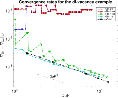
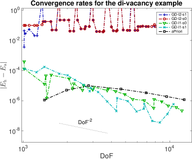
Refer to caption
Figure 3. Numerical results by Algorithm 5.2: H1superscript𝐻1H^{1} error vs. N𝑁N, using a posteriori estimator in H1superscript𝐻1H^{1} norm. In the legend, l1 means 1superscript1\ell^{1}-minimization approach while l2 represents a least-squares approach; s1 indicates with stabilization and s0 without.
Refer to caption
Figure 4. Numerical results by Algorithm 5.2: Energy error vs. N𝑁N, using a posteriori estimator in H1superscript𝐻1H^{1} norm. In the legend, l1 means 1superscript1\ell^{1}-minimization approach while l2 represents a least-squares approach; s1 indicates with stabilization and s0 without.
Refer to caption
Figure 5. Numerical results by Algorithm 5.2: H1superscript𝐻1H^{1} error vs. N𝑁N, using a posteriori estimator in H1superscript𝐻1H^{1} norm. In the legend, l1 means 1superscript1\ell^{1}-minimization approach while l2 represents a least-squares approach; s1 indicates with stabilization and s0 without.
Refer to caption
Figure 6. Numerical results by Algorithm 5.2: Energy error vs. N𝑁N, using a posteriori estimator in H1superscript𝐻1H^{1} norm. In the legend, l1 means 1superscript1\ell^{1}-minimization approach while l2 represents a least-squares approach; s1 indicates with stabilization and s0 without.

6. Conclusion

In this paper, we construct the adaptive algorithm for a class of consistent (ghost force free) atomistic/continuum coupling schemes with finite range interactions based on the rigorous a posteriori error estimates. Different from the localization formula for the stress tensor in the a priori analysis [21, 23, 26], we develop a computable formulation for the stress tensor. Combined with 1subscript1\ell_{1}-minimization approach for reconstruction parameters and stabilization, we have shown that the numerical results for the corresponding adaptive algorithms are comparable to optimal a priori analysis.

The extension of the straight screw dislocation in two dimensions and point defect case in three dimensions is straightforward. More practical problems, for example, the study of dislocation nucleation and dislocation interaction by a/c coupling methods has attracted considerable attention from the early stage of a/c coupling methods [37, 31]. The difficulty is to deal with boundary condition and complicated geometry changes of the interface.

For general atomistic/continuum coupling schemes, such as BQCE, BQCF and BGFC, the a priori analysis in [15, 12, 30] provide a general analytical framework and the stress tensor based formulation plays a key role in the analysis. Therefore, the a posteriori analysis for those coupling schemes can inherit this analytical framework and the stress tensor formulation. Techniques developed in this paper will be essential for the efficient implementation of the corresponding adaptive algorithms.

7. Appendix

7.1. Derivation of (4.8) for Two Dimensional Triangular Lattice

In this section, for two dimensional triangular lattice introduced in § 5.2, we derive (4.8). We first classify interaction bonds into two types according to their intersection to corresponding elements.

Type I interaction bonds is parallel to one of the nearest neighbour directions. The set of all Type I bonds is defined by BI={ρ|ainn, such that ρ=|ρ|ai}subscriptBIconditional-set𝜌formulae-sequencesubscripta𝑖subscriptnn such that 𝜌𝜌subscript𝑎𝑖\textsf{B}_{\textrm{I}}=\{\rho|\exists\textrm{a}_{i}\in\mathcal{R}_{\textrm{nn}},\text{ such that }\rho=|\rho|a_{i}\}, as illustrated in Figure 7.

Refer to caption
Figure 7. Illustration of corresponding elements (marked gray) to bond ρBI𝜌subscriptBI\rho\in\textsf{B}_{\textrm{I}} with ρ=2a3𝜌2subscript𝑎3\rho=2a_{3}.

For each ρBI𝜌subscriptBI\rho\in\textsf{B}_{\textrm{I}} with start point ΛΛ\ell\in\Lambda and v𝒰1,2𝑣superscript𝒰12v\in\mathscr{U}^{1,2}, we have

Dρvsubscript𝐷𝜌𝑣\displaystyle D_{\rho}v =k=1|ρ|Daiv(+(k1)ai)absentsuperscriptsubscript𝑘1𝜌subscript𝐷subscript𝑎𝑖𝑣𝑘1subscript𝑎𝑖\displaystyle=\sum_{k=1}^{|\rho|}D_{a_{i}}v(\ell+(k-1)a_{i})
=(k=1|ρ|(12Tk+v+12Tkv))ρ|ρ|absentsuperscriptsubscript𝑘1𝜌12subscriptsuperscriptsubscript𝑇𝑘𝑣12subscriptsuperscriptsubscript𝑇𝑘𝑣𝜌𝜌\displaystyle=\left(\sum_{k=1}^{|\rho|}\left(\frac{1}{2}\nabla_{T_{k}^{+}}v+\frac{1}{2}\nabla_{T_{k}^{-}}v\right)\right)\cdot\frac{\rho}{|\rho|} (7.1)
=k=1|ρ|12|ρ|(Tk+vρ+Tkvρ)absentsuperscriptsubscript𝑘1𝜌12𝜌subscriptsuperscriptsubscript𝑇𝑘𝑣𝜌subscriptsuperscriptsubscript𝑇𝑘𝑣𝜌\displaystyle=\sum_{k=1}^{|\rho|}\frac{1}{2|\rho|}\left(\nabla_{T_{k}^{+}}v\cdot\rho+\nabla_{T_{k}^{-}}v\cdot\rho\right)

where Tk+superscriptsubscript𝑇𝑘T_{k}^{+} and Tksuperscriptsubscript𝑇𝑘T_{k}^{-} are the triangles with (+(k1)ai,+kai)𝑘1subscript𝑎𝑖𝑘subscript𝑎𝑖\left(\ell+(k-1)a_{i},\ell+ka_{i}\right) as the common edge, for k=1,,|ρ|𝑘1𝜌k=1,\ldots,|\rho|, superscript “++” means the element being located on the left of the bond. In this case, the contribution in(4.8) is

ωρ(Tk(±))=12|ρ|.superscriptsubscript𝜔𝜌superscriptsubscript𝑇𝑘plus-or-minus12𝜌\omega_{\ell}^{\rho}(T_{k}^{(\pm)})=\frac{1}{2|\rho|}.

Type II interaction bonds is not parallel to any of the nearest neighbour directions, therefore they must cross the intersecting elements. The set of all Type II bonds is defined by BII={ρ|ρ is not parallel to any ainn}subscriptBIIconditional-set𝜌𝜌 is not parallel to any subscript𝑎𝑖subscriptnn\textsf{B}_{\textrm{II}}=\{\rho|\rho\text{ is not parallel to any }a_{i}\in\mathcal{R}_{\textrm{nn}}\}, as illustrated in Figure 8.

Refer to caption
Figure 8. Illustration of the intersecting elements (marked gray) with respect to bond ρBII𝜌subscriptBII\rho\in\textsf{B}_{\textrm{II}}, ρ=a1+2a2𝜌subscript𝑎12subscript𝑎2\rho=a_{1}+2a_{2}.

For any Type II interaction bond ρBII𝜌subscriptBII\rho\in\textsf{B}_{\textrm{II}}, there exists nearest neighbour directions aisubscript𝑎𝑖a_{i}, ai+1subscript𝑎𝑖1a_{i+1}, such that ρ=αai+βai+1𝜌𝛼subscript𝑎𝑖𝛽subscript𝑎𝑖1\rho=\alpha a_{i}+\beta a_{i+1}, α,β>0𝛼𝛽0\alpha,\beta>0. Let (,+ρ)𝜌(\ell,\ell+\rho) consecutively intersect with elements Tksubscript𝑇𝑘T_{k}, k=1,,np𝑘1subscript𝑛𝑝k=1,\cdots,n_{p}, for v𝒰1,2𝑣superscript𝒰12v\in\mathscr{U}^{1,2}, we have

Dρvsubscript𝐷𝜌𝑣\displaystyle D_{\rho}v =ρV(k=1nρDρkv(+t=1kρk1))absentsubscript𝜌subscript𝑉superscriptsubscript𝑘1subscript𝑛𝜌subscript𝐷subscript𝜌𝑘𝑣superscriptsubscript𝑡1𝑘subscript𝜌𝑘1\displaystyle=\partial_{\rho}V_{\ell}\left(\sum_{k=1}^{n_{\rho}}D_{\rho_{k}}v(\ell+\sum_{t=1}^{k}\rho_{k-1})\right)
=(k=1nρTkv)ρkabsentsuperscriptsubscript𝑘1subscript𝑛𝜌subscriptsubscript𝑇𝑘𝑣subscript𝜌𝑘\displaystyle=\left(\sum_{k=1}^{n_{\rho}}\nabla_{T_{k}}v\right)\cdot\rho_{k} (7.2)
=(k=1nρTkv)|ρk||ρ|ρabsentsuperscriptsubscript𝑘1subscript𝑛𝜌subscriptsubscript𝑇𝑘𝑣subscript𝜌𝑘𝜌𝜌\displaystyle=\left(\sum_{k=1}^{n_{\rho}}\nabla_{T_{k}}v\right)\cdot\frac{|\rho_{k}|}{|\rho|}\rho
=k=1nρ)|ρk||ρ|Tkvρ\displaystyle=\sum_{k=1}^{n_{\rho})}\frac{|\rho_{k}|}{|\rho|}\nabla_{T_{k}}v\cdot\rho

where the set of vectors {ρk}k=1nρsuperscriptsubscriptsubscript𝜌𝑘𝑘1subscript𝑛𝜌\{\rho_{k}\}_{k=1}^{n_{\rho}} is the unit partition of ρ𝜌\rho with ρ=k=1nρρk𝜌superscriptsubscript𝑘1subscript𝑛𝜌subscript𝜌𝑘\rho=\sum_{k=1}^{n_{\rho}}\rho_{k}, ρ0=𝟎subscript𝜌00\rho_{0}=\mathbf{0} and ρk|ρk|=ρ|ρ|subscript𝜌𝑘subscript𝜌𝑘𝜌𝜌\frac{\rho_{k}}{|\rho_{k}|}=\frac{\rho}{|\rho|} for k=1,,np𝑘1subscript𝑛𝑝k=1,\ldots,n_{p}. ρk=Tk(,+ρ)subscript𝜌𝑘subscript𝑇𝑘𝜌\rho_{k}=T_{k}\cap(\ell,\ell+\rho). For the two dimensional triangular lattice as in § 5.2, we have nρ=2(α+β1)subscript𝑛𝜌2𝛼𝛽1n_{\rho}=2(\alpha+\beta-1) if αβ𝛼𝛽\alpha\neq\beta, and nρ=2αsubscript𝑛𝜌2𝛼n_{\rho}=2\alpha if α=β𝛼𝛽\alpha=\beta. In this case,

ωρ(Tk)=|ρk||ρ|.superscriptsubscript𝜔𝜌subscript𝑇𝑘subscript𝜌𝑘𝜌\omega_{\ell}^{\rho}(T_{k})=\frac{|\rho_{k}|}{|\rho|}.

For the Type II bonds with α=β𝛼𝛽\alpha=\beta, in the hexagon site geometry, The contribution factor ωρTsuperscriptsubscript𝜔𝜌𝑇\omega_{\rho}^{T} is the same for every element related to bond ρ𝜌\rho with the value ωρT=12αsuperscriptsubscript𝜔𝜌𝑇12𝛼\omega_{\rho}^{T}=\frac{1}{2\alpha} which can be see from figure (9).

Refer to caption
Figure 9. Illustration of corresponding elements (marked gray) to bond ρBI𝜌subscriptBI\rho\in\textsf{B}_{\textrm{I}} with ρ=2a1+2a2𝜌2subscript𝑎12subscript𝑎2\rho=2a_{1}+2a_{2}.

References

  • [1] M. Arndt and M. Luskin. Error estimation and atomistic-continuum adaptivity for the quasicontinuum approximation of a Frenkel-Kontorova model. SIAM J. Multiscale Modeling & Simulation, 7:147–170, 2008.
  • [2] M. Arndt and M. Luskin. Goal-oriented adaptive mesh refinement for the quasicontinuum approximation of a Frenkel-Kontorova model. Computer Methods in Applied Mechanics and Engineering, 197:4298–4306, 2008.
  • [3] H. Chen and C. Ortner. Qm/mm methods for crystalline defects. part 1: Locality of the tight binding model. Multiscale Model. Simul., 14:232–264, 2016.
  • [4] H. Chen and C. Ortner. Qm/mm methods for crystalline defects. part 2: Consistent energy and force-mixing. Multiscale Model. Simul., 15:184–214, 2017.
  • [5] M. S. Daw and M. I. Baskes. Embedded-Atom Method: Derivation and Application to Impurities, Surfaces, and other Defects in Metals. Physical Review B, 20, 1984.
  • [6] W. Dörfler. A convergent adaptive algorithm for poisson’s equation. SIAM J. Numer. Anal., 33:1106–1124, 1996.
  • [7] W. E, J. Lu, and J. Z. Yang. Uniform accuracy of the quasicontinuum method. Phys. Rev. B, 74(21):214115, 2006.
  • [8] W. E and P. Ming. Cauchy-Born rule and the stability of crystalline solids: static problems. Arch. Ration. Mech. Anal., 183(2):241–297, 2007.
  • [9] V. Ehrlacher, C. Ortner, and A. V. Shapeev. Analysis of boundary conditions for crystal defect atomistic simulations. Arch. Rat. Mech. Anal., 222(3):1217–1268, 2016.
  • [10] M. W. Finnis and J. E. Sinclair. A simple empirical n-body potential for transition-metals. Philos. Mag. A, 50(1):45–55, 1984.
  • [11] H. Fischmeister, H. Exner, M.-H. Poech, S. Kohlhoff, P. Gumbsch, S. Schmauder, L. S. Sigi, and R. Spiegler. Modelling fracture processes in metals and composite materials. Z. Metallkde., 80:839–846, 1989.
  • [12] X. H. Li, C. Ortner, A. V. Shapeev, and B. Van Koten. Analysis of blended atomistic/continuum hybrid methods. Numerische Mathematik, 134(2):275–326, 2016.
  • [13] Lei Zhang Lidong Fang, Apala Majumdar. Multiscale numerical method for nematic liquid crystal. 2018.
  • [14] P. Lin. Convergence analysis of a quasi-continuum approximation for a two-dimensional material without defects. SIAM J. Numer. Anal., 45(1):313–332 (electronic), 2007.
  • [15] J. Lu and P. Ming. Convergence of a force-based hybrid method for atomistic and continuum models in three dimension. Comm. Pure Appl. Math., 66:83–108, 2013.
  • [16] M. Luskin and C. Ortner. Atomistic-to-continuum-coupling. Acta Numerica, 2013.
  • [17] M. Luskin, C. Ortner, and B. Van Koten. Formulation and optimization of the energy-based blended quasicontinuum method. Comput. Methods Appl. Mech. Engrg., 253, 2013.
  • [18] R. Miller and E. Tadmor. A unified framework and performance benchmark of fourteen multiscale atomistic/continuum coupling methods. Modelling Simul. Mater. Sci. Eng., 17, 2009.
  • [19] M. Ortiz, R. Phillips, and E. B. Tadmor. Quasicontinuum analysis of defects in solids. Philosophical Magazine A, 73(6):1529–1563, 1996.
  • [20] C. Ortner. A priori and a posteriori analysis of the quasi-nonlocal quasicontinuum method in 1D. Math. Comp., 80(275):1265–1285, 2011.
  • [21] C. Ortner. The role of the patch test in 2D atomistic-to-continuum coupling methods. ESAIM Math. Model. Numer. Anal., 46, 2012.
  • [22] C. Ortner, A. Shapeev, and L. Zhang. (in-)stability and stabilisation of qnl-type atomistic-to-continuum coupling methods. SIAM Multiscale Model. Simul., 12(3):1258–1293, 2014.
  • [23] C. Ortner and A. V. Shapeev. Interpolation of lattice functions and applications to atomistic/continuum multiscale methods. ArXiv e-prints, arXiv:1204.3705, 2012.
  • [24] C. Ortner and A. V. Shapeev. Analysis of an energy-based atomistic/continuum coupling approximation of a vacancy in the 2d triangular lattice. Math. Comp., 82:2191–2236, 2013.
  • [25] C. Ortner and E. Süli. Analysis of a quasicontinuum method in one dimension. M2AN Math. Model. Numer. Anal., 42(1):57–91, 2008.
  • [26] C. Ortner and F. Theil. Justification of the cauchy–born approximation of elastodynamics. Arch. Ration. Mech. Anal., 207, 2013.
  • [27] C. Ortner and H. Wang. A posteriori error control for a quasi-continuum approximation of a periodic chain. IMA Journal of Numerical Analysis, 34(3):977–1001, 2013.
  • [28] C. Ortner and L. Zhang. Construction and sharp consistency estimates for atomistic/continuum coupling methods with general interfaces: a 2D model problem. SIAM J. Numer. Anal., 50, 2012.
  • [29] C. Ortner and L. Zhang. Energy-based atomisitic-to-continuum coupling without ghost forces. Comput. Methods Appl. Mech. Engrg., 279(1):29–45, 2014.
  • [30] C. Ortner and L. Zhang. Atomistic/continuum blending with ghost force correction. SIAM J. Sci. Comput., 38(1):A346–A375, 2016.
  • [31] R. Phillips, D. Rodney, V. Shenoy, E. Tadmor, and M. Ortiz. Hierarchical models of plasticity: dislocation nucleation and interaction. Modelling Simul. Mater. Sci. Eng., 7:769–780, 1999.
  • [32] S. Prudhomme, P. T. Bauman, and J. T. Oden. Error control for molecular statics problems. International Journal for Multiscale Computational Engineering, 4(5-6):647–662, 2006.
  • [33] A. V. Shapeev. Consistent energy-based atomistic/continuum coupling for two-body potentials in one and two dimensions. Multiscale Modeling & Simulation, 9(3):905–932, 2011.
  • [34] A. V. Shapeev. Consistent energy-based atomistic/continuum coupling for two-body potentials in three dimensions. SIAM J. Sci. Comput., 34(3):B335–B360, 2012.
  • [35] V. B. Shenoy, R. Miller, E. B. Tadmor, D. Rodney, R. Phillips, and M. Ortiz. An adaptive finite element approach to atomic-scale mechanics–the quasicontinuum method. J. Mech. Phys. Solids, 47(3):611–642, 1999.
  • [36] T. Shimokawa, J. J. Mortensen, J. Schiotz, and K. W. Jacobsen. Matching conditions in the quasicontinuum method: Removal of the error introduced at the interface between the coarse-grained and fully atomistic region. Phys. Rev. B, 69(21):214104, 2004.
  • [37] E. B. Tadmor, R. Miller, R. Phillips, and M. Ortiz. Nanoindentation and incipient plasticity. Journal of Materials Research, 14(6):2233–2250, 1999.
  • [38] E. B. Tadmor and R. E. Miller. Modeling Materials: Continuum, Atomistic and Multiscale Techniques. Cambridge University Press, 2012.
  • [39] I. Tembhekar, J. S. Amelang, L. Munk, and D. M. Kochmann. Automatic adaptivity in the fully-nonlocal quasicontinuum method for coarse-grained atomistic simulations. Int. J. Numer. Meth. Engng., 2016.
  • [40] H. Wang, M. Liao, P. Lin, and L. Zhang. A posteriori error estimation and adaptive algorithm for the atomistic/continuum coupling in 2d. ArXiv e-prints, arXiv:1702.02701, 2017.