KUNS-2732

Emergence of AdS geometry
in the simulated tempering algorithm

Masafumi Fukuma¹, Nobuyuki Matsumoto¹ and Naoya Umeda²

¹Department of Physics, Kyoto University, Kyoto 606-8502, Japan
²PricewaterhouseCoopers Aarata LLC,
Otemachi Park Building, 1-1-1 Otemachi, Chiyoda-ku, Tokyo 100-0004, Japan

In our previous work [1], we introduced to an arbitrary Markov chain Monte Carlo algorithm a distance between configurations. This measures the difficulty of transition from one configuration to the other, and enables us to investigate the relaxation of probability distribution from a geometrical point of view. In this paper, we investigate the global geometry of a stochastic system whose equilibrium distribution is highly multimodal with a large number of degenerate vacua. We show that, when the simulated tempering algorithm is implemented to such a system, the extended configuration space has an asymptotically Euclidean anti-de Sitter (AdS) geometry. We further show that this knowledge of geometry enables us to optimize the tempering parameter in a simple, geometrical way.

1 Introduction

Let $\mathcal{M}=\{x\}$ be a configuration space, and $S(x)$ an action. We are often concerned with calculating the vacuum expectation value (VEV) of an operator $\mathcal{O}(x)$ with respect to the action:

$$\langle\mathcal{O}(x)\rangle\equiv\frac{1}{Z}\,\int dx\,e^{-S(x)}\,\mathcal{O}(x)\quad\Bigl{(}Z=\int dx\,e^{-S(x)}\Bigr{)}.$$ (1.1)

In a Markov chain Monte Carlo (MCMC) simulation, we set up an algorithm that generates a stochastic process $p_{n}(x)\to p_{n+1}(x)=\int dy\,P(x|y)\,p_{n}(y)$ such that the probability distribution $p_{n}(x)$ relaxes to the desired equilibrium distribution $e^{-S(x)}/Z$ in the limit $n\to\infty$. In order for such an algorithm to be practically useful, the relaxation to equilibrium needs to be sufficiently rapid. However, when the equilibrium distribution is multimodal (i.e., when the action has very high potential barriers), transitions between configurations belonging to different modes take extraordinarily long computational times, which delay the relaxation to equilibrium and make the MCMC simulation almost impractical.

To accelerate the transitions, there have been invented various methods, including the overrelaxation [2] and the simulated and the parallel tempering methods [3, 4, 5, 6]. In the simulated tempering method [3], for example, as will be briefly reviewed in subsection 3.1, one picks up a parameter $\beta$ of the model (such as the overall coefficient of the action) as a tempering parameter, and extends the configuration space by treating $\beta$ as an additional dynamical variable. We then design a MCMC algorithm such that configurations belonging to different modes for the original action now can be connected easily by passing through configurations in the extended configuration space. In order for such an algorithm to work, transitions along the $\beta$ direction must have significant acceptance rates, which enforces us to make a careful adjustment of the parameters that are additionally introduced when extending the configuration space.

In our previous work [1], we introduced to an arbitrary MCMC algorithm the notion of distance between configurations. This measures the difficulty of transition from one configuration to the other, and enables us to investigate the relaxation of probability distribution from a geometrical point of view. We also introduced the coarse-grained configuration space to a highly multimodal stochastic system, where configurations in the same mode are regarded as a single configuration [1]. This perspective facilitates the understanding of the global geometry of the configuration space, and is justified by the fact that distances between different modes take so large values that the difference of distances between two configurations in the same mode can be effectively neglected. In this paper, we investigate the global geometry of such a highly multimodal stochastic system with a large number of degenerate vacua. We show that, when the simulated tempering algorithm is implemented, an asymptotically Euclidean anti-de Sitter (AdS) geometry emerges in the extended, coarse-grained configuration space. We further show that this knowledge of geometry enables us to optimize the additional parameters in a simple, geometrical way.

This paper is organized as follows. In section 2, we give a brief review on the distance between configurations for a MCMC algorithm [1]. We mainly consider a system whose equilibrium distribution is highly multimodal with a large number of degenerate vacua. We also introduce the concept of the coarse-grained configuration space and define the metric on the space. In section 3, we implement the simulated tempering method by taking the tempering parameter to be the overall coefficient of the action, and show that the geometry of the extended, coarse-grained configuration space is given by an asymptotically Euclidean AdS space metric. In Section 4, we optimize the tempering parameter such that the distances get minimized, and show that this can be easily done in a geometrical way. The conclusion is confirmed by direct numerical calculations. Section 5 is devoted to conclusion and outlook for future work.

2 Distance between configurations in MCMC simulations

In this section, we give a brief review on the distance between configurations for a MCMC algorithm [1]. We mainly consider a system whose equilibrium distribution is highly multimodal with a large number of degenerate vacua. We then introduce the coarse-grained configuration space, where configurations in the same mode are regarded as a single configuration.

2.1 Definition of the distance between configurations

Let us consider a configuration space $\mathcal{M}=\{x\}$ with a real-valued action $S(x)$. Suppose that we make a numerical simulation to estimate the VEVs of observables by using a given MCMC algorithm. We denote by $P(x|y)=\langle x|\hat{P}\,|y\rangle$ the transition probability from a configuration $y$ to a configuration $x$ at a single Markov step. The Markov property then says that the transition probability from $y$ to $x$ at $n$ steps is given by $P_{n}(x|y)=\langle x|\hat{P}^{n}|y\rangle$. We assume that the stochastic process has the unique equilibrium distribution $e^{-S(x)}/Z$ $(Z=\int dxe^{-S(x)})$ and $P(x|y)$ satisfies the detailed balance condition $P(x|y)\,e^{-S(y)}=P(y|x)\,e^{-S(x)}$. We further assume that all the eigenvalues of $P(x|y)$ are positive (see [1] for mathematical details).

The distance $\theta_{n}(x,y)$ between two configurations $x,y$ [1] is then defined by

$$\theta_{n}(x,y)\equiv\arccos\biggl{(}\frac{P_{n}(x|y)\,P_{n}(y|x)}{P_{n}(x|x)\,P_{n}(y|y)}\biggr{)}.$$ (2.1)

One can easily show that $\theta_{n}(x,y)$ satisfies the axioms of distance [1]:

$$\bullet \ \theta_{n}(x,y)\geq 0,$$ (2.2)

$$\bullet \ x=y\Leftrightarrow\theta_{n}(x,y)=0,$$ (2.3)

$$\bullet \ \theta_{n}(x,y)=\theta_{n}(y,x),$$ (2.4)

$$\bullet \ \theta_{n}(x,y)+\theta_{n}(y,z)\geq\theta_{n}(x,z),$$ (2.5)

and vanishes in the limit $n\to\infty$ for any two configurations $x,\,y\in\mathcal{M}$:

$$\lim_{n\to\infty}\,\theta_{n}(x,y)=0,$$ (2.6)

because $P_{n}(x|y)\to e^{-S(x)}/Z$ in the limit $n\to\infty$. The distance $\theta_{n}(x,y)$ actually measures the difficulty of transition from $y$ to $x$ at $n$ steps in the sense that:

• When configurations $x$ and $y$ belong to different modes of the equilibrium distribution, $\theta_{n}(x,y)$ is large for a finite $n$.

• If $x$ can be easily reached from $y$, $\theta_{n}(x,y)$ is small even for a finite $n$.

One can further show that, as long as the chosen algorithm generates only local moves of configuration, the large scale structure of distance $\theta_{n}(x,y)$ takes a universal form, in the sense that differences of distance between two such algorithms can always be absorbed into a rescaling of $n$ [1].

In [1] we introduced a few distances in addition to $\theta_{n}(x,y)$, among which is the distance $d_{n}(x,y)$ that is defined by

$$d_{n}(x,y)=\sqrt{-\log\biggl{(}\frac{P_{n}(x|y)\,P_{n}(y|x)}{P_{n}(x|x)\,P_{n}(y|y)}\biggr{)}}$$ (2.7)

and is related with $\theta_{n}(x,y)$ as

$$\cos\theta_{n}(x,y)=e^{-(1/2)\,d_{n}^{2}(x,y)}.$$ (2.8)

$d_{n}(x,y)$ agrees with $\theta_{n}(x,y)$ when they take small values, and satisfies almost the same properties as $\theta_{n}(x,y)$. The only exception is that $d_{n}(x,y)$ generically does not satisfy the triangle inequality for the original configuration space $\mathcal{M}$. However, as will be discussed in subsection 2.3, $d_{n}(x,y)$ is more useful than $\theta_{n}(x,y)$ for investigating the large scale geometry of the configuration space and does satisfy the triangle inequality when the configuration space is coarse-grained. Thus, we will mainly use $d_{n}(x,y)$ in the following discussions.

2.2 Coarse-grained configuration space

For a stochastic system whose equilibrium distribution is highly multimodal with a large number of degenerate vacua, distances $d_{n}$ between two different modes take so large values that the difference of distances between two configurations in the same mode can be effectively neglected. This leads us to introduce the coarse-grained configuration space $\bar{\mathcal{M}}$ by regarding configurations in the same mode as a single configuration [1]. In the following, we assume that a way of separation between different modes is uniform and translationally invariant in $\bar{\mathcal{M}}$. A typical model which has this property can be given by the action

$$S(\mathbf{x};\beta_{0})=\beta_{0}\,\sum_{\mu=1}^{D}\,[1-\cos(2\pi x_{\mu})].$$ (2.9)

Here, the configuration space is a $D$-dimensional torus with the period $2L$ for every direction: $\mathcal{M}=\{\mathbf{x}=(x_{\mu})\,|\,{-L}<x_{\mu}\leq L\ (\mu=1,\ldots,D)\}$ (we impose the periodic boundary condition). This action certainly gives a multimodal equilibrium distribution when $\beta_{0}\gg 1$. The coarse-grained configuration space $\bar{\mathcal{M}}$ is given by the $D$-dimensional lattice torus $\bar{\mathcal{M}}=\{n=(n_{\mu})\,|\,n_{\mu}={-L}+1,\ldots,L-1,L\}$, that consists of the degenerate classical vacua and has a translational invariance.

2.3 Distance on the coarse-grained configuration space

We here explain why we think that $d_{n}(x,y)$ is more suitable than $\theta_{n}(x,y)$ for investigating the geometry of $\bar{\mathcal{M}}$.

Firstly, $d_{n}(x,y)$ has a better resolution on the large scale structure of configuration space. In fact, as can be seen from its definition, when transitions between two configurations $x$ and $y$ happen only very rarely, $d_{n}(x,y)$ can take a large value without limitation, while the value of $\theta_{n}(x,y)$ is saturated close to $\pi/2$.

Secondly, the distance $d_{n}(x,y)$ gives a flat Euclidean metric for a simple Gaussian distribution [1]. In fact, for a quadratic action $S(\mathbf{x})=(\omega/2)\,\mathbf{x}^{2}$ defined on the configuration space $\mathcal{M}=\{\mathbf{x}\,|\,\mathbf{x}\in\mathbb{R}^{D}\}$ with the Langevin algorithm, the distance between $\mathbf{x}$ and $\mathbf{y}$ is given by

$$d_{n}(\mathbf{x},\mathbf{y})=\sqrt{\frac{\omega}{2\sinh(\omega n\epsilon)}}\,|\mathbf{x}-\mathbf{y}|,$$ (2.10)

where $\epsilon$ is the step size of the discretized fictitious time in the Langevin equation. $\theta_{n}(x,y)$, to the contrary, has a complicated expression.

Lastly, the distance $d_{n}(x,y)$ is expected to satisfy the triangle inequality on the coarse-grained configuration space $\bar{\mathcal{M}}$. Although we still do not have a rigorous proof on this statement, we can check it numerically for the model (2.9). To see this, we first note that the triangle inequality in $\bar{\mathcal{M}}$ is equivalent to the concavity of $d_{n}(x,y)$ as a function of $r=|x-y|$ ($x,y\in\bar{\mathcal{M}}$) due to the translational symmetry of this model. Figure 1 shows $d_{n}(x,0)$ for the action (2.9) with $D=1$, $L=10$ and $\beta_{0}=3$.

Figure 1: $d_{n}(x,0)$ for $0\leq x\leq L$. We set $n=2,500$ , $\beta_{0}=3$ and $L=10$.

As a MCMC algorithm, we use the Metropolis algorithm with the Gaussian proposal distribution with standard deviation $\sigma_{x}=1.6/(2\pi\sqrt{\beta_{0}})$. We discretize the original configuration space $\mathcal{M}$ with spacing $0.02$, and numerically construct the transition matrix $P(x|y)$. We then calculate $d_{n}(x,0)$ for $0\leq x\leq L$ with $n=2,500$. We see that, although $d_{n}(x,0)$ does not satisfy concavity for generic configurations $x\in\mathcal{M}$, it becomes a concave function of $r=|x|$ when $x$ is on the lattice of the coarse-grained configuration space (drawn as orange points in the figure).

We now define the metric $ds^{2}$ in the coarse-grained configuration space $\bar{\mathcal{M}}$ as

$$ds^{2}\equiv d_{n}^{2}(x,\,x+dx),$$ (2.11)

where $x$ and $x+dx$ are nearby points residing on $\bar{\mathcal{M}}$ [1]. For the translationally invariant, parity even action (2.9), the metric will take the following form for $\beta_{0}\gg 1$:

$$ds^{2}={\rm const.}\,\beta_{0}\,\sum_{\mu=1}^{D}\,dx_{\mu}^{2},$$ (2.12)

because the transition probability between two neighboring modes is given by $O(e^{-{\rm const.}\,\beta_{0}})$ as can be easily seen by an instanton calculus [1].

3 Emergence of the Euclidean AdS geometry

In this section, we implement the simulated tempering method for the action (2.9) by taking the tempering parameter to be the overall coefficient of the action, $\beta_{0}$. The configuration space is thus extended so that the tempering parameter is also treated as a dynamical variable. We show that the global geometry of the extended configuration space is given by an asymptotically Euclidean AdS metric. In subsection 3.1 we briefly explain the simulated tempering algorithm, and in subsection 3.2 we write down the transition matrix explicitly for large $\beta$. In subsection 3.3 we prove that the geometry of the extended, coarse-grained configuration space is given by an AdS metric for large $\beta$. This statement is numerically verified in subsection 3.4.

3.1 Simulated tempering algorithm

We here give a brief review of the simulated tempering algorithm [3]. As is commented in Introduction, this is introduced to a multimodal stochastic system in order to accelerate the relaxation to global equilibrium.

A MCMC simulation proceeds as follows:

1. We choose a tempering parameter (to be denoted by $\beta_{0}$) from parameters in the action, which we write as $S(x;\beta_{0})$ to indicate its dependence on $\beta_{0}$.

2. We introduce the tempering parameter set $\mathcal{A}=\{\beta_{a}\}$ $(a=0,1,\ldots,A)$, to which belongs the original parameter $\beta_{0}$.

3. We extend the original configuration space $\mathcal{M}=\{x\}$ to $\mathcal{M}\times\mathcal{A}=\{X=(x,\beta_{a})\}$.

4. We set up a Markov chain on the extended configuration space such that the global equilibrium distribution $P_{\rm eq}(X)$ takes the form

   $$P_{\rm eq}(X)=P_{\rm eq}(x,\beta_{a})=w_{a}\,e^{-S(x;\beta_{a})}.$$ (3.1)

5. After the system is well regarded as reaching global equilibrium, we retrieve a subsample with $\beta_{a=0}$ out of a full sample taken from the extended configuration space, and estimate the VEVs by sample averages with respect to the subsample.

In this paper, we realize the global equilibrium (3.1) by repeating the following steps:

• We generate a local move in the $x$ direction, $X=(x,\beta_{a})\to X^{\prime}=(x^{\prime},\beta_{a})$, with the Metropolis algorithm. This is repeated $2k$ times so that local equilibrium is realized for fixed $\beta_{a}$.

• We generate a local move in the $\beta$ direction, $X=(x,\beta_{a})\to X^{\prime}=(x,\beta_{a\pm 1})$, using the Metropolis algorithm, where an adjacent tempering parameter is proposed with probability $1/2$ and accepted with probability $\min(1,P_{\mathrm{eq}}(X^{\prime})/P_{\mathrm{eq}}(X))$.

We denote by $\hat{P}_{(1)}$ the one-step transition matrix in the $x$ direction, which will be repeated $2k$ times, and by $\hat{P}_{(2)}$ that in the $\beta$ direction. We regard

$$\hat{P}\equiv\hat{P}_{(1)}^{k}\hat{P}_{(2)}\hat{P}_{(1)}^{k}$$ (3.2)

as the transition matrix at a single Markov step. One can easily check that $\hat{P}$ satisfies the detailed balance condition, $\langle X|\hat{P}|X^{\prime}\rangle\,P_{\rm eq}(X^{\prime})=\langle X^{\prime}|\hat{P}|X\rangle\,P_{\rm eq}(X)$.

With the transition matrix $\hat{P}$, the distance $d_{n}(X,Y)$ is defined for the extended configuration space $\mathcal{M}\times\mathcal{A}$ as in (2.7):

$$d_{n}(X,Y)=\sqrt{-\log\biggl{(}\frac{P_{n}(X|Y)\,P_{n}(Y|X)}{P_{n}(X|X)\,P_{n}(Y|Y)}\biggr{)}},$$ (3.3)

where $P_{n}(X|Y)=\langle X|\hat{P}^{n}|Y\rangle$. In appendix A, we demonstrate that the distance $d_{n}(X,Y)$ also satisfies the triangle inequality on the extended, coarse-grained configuration space $\bar{\mathcal{M}}\times\mathcal{A}$.

3.2 Matrix elements of the transition matrix

In this subsection, we write down the matrix elements of $\hat{P}=\hat{P}_{(1)}^{k}\hat{P}_{(2)}\hat{P}_{(1)}^{k}$ for $\beta_{a},\beta_{b}\gg 1$:

$$\langle\mathbf{x},\beta_{a}\,|\,\hat{P}\,|\,\mathbf{y},\beta_{b}\rangle =\langle\mathbf{x},\beta_{a}\,|\,\hat{P}_{(1)}^{k}\hat{P}_{(2)}\hat{P}_{(1)}^{k}\,|\,\mathbf{y},\beta_{b}\rangle$$

$$=\int_{\mathcal{M}}d^{D}x_{1}d^{D}x_{2}\,\sum_{a_{1},a_{2}}\langle\mathbf{x},\beta_{a}\,|\,\hat{P}_{(1)}^{k}\,|\,\mathbf{x}_{1},\beta_{a_{1}}\rangle\times$$

$$~{}~{}~{}~{}\times\langle\mathbf{x}_{1},\beta_{a_{1}}\,|\,\hat{P}_{(2)}\,|\,\mathbf{x}_{2},\beta_{a_{2}}\rangle\,\langle\mathbf{x}_{2},\beta_{a_{2}}\,|\,\hat{P}_{(1)}^{k}\,|\,\mathbf{y},\beta_{b}\rangle.$$ (3.4)

We first recall that $k$ is taken to be sufficiently large such that the transition in the $x$ direction, $\hat{P}_{(1)}^{k}$, makes the system be well in local equilibrium. Thus, configurations will get distributed around local minima after the action of $\hat{P}_{(1)}^{k}$,

$$\langle\mathbf{x},\beta_{a}\,|\,\hat{P}_{(1)}^{k}\,|\,\mathbf{y},\beta_{b}\rangle\simeq P_{\mathrm{eq}}^{(\mathrm{loc})}(\mathbf{x},\beta_{a})\,\delta_{[\mathbf{x}]\,[\mathbf{y}]}\,\delta_{ab}\quad(\beta_{a},\beta_{b}\gg 1).$$ (3.5)

Here, $[\mathbf{x}]$ represents the local minimum (a lattice point) within the mode to which $\mathbf{x}$ belongs. The probability distribution of local equilibrium, $P_{\mathrm{eq}}^{(\mathrm{loc})}(\mathbf{x},\beta_{a})$, should be well approximated by the Gaussian distribution around $[\mathbf{x}]$ for large $\beta_{a}$:

$$P_{\mathrm{eq}}^{(\mathrm{loc})}(\mathbf{x},\beta_{a})\simeq(2\pi\beta_{a})^{D/2}\,e^{-2\pi^{2}\beta_{a}\,|\mathbf{x}-[\mathbf{x}]|^{2}}.$$ (3.6)

On the other hand, the matrix elements of $\hat{P}_{(2)}$ for $a\neq b$ are given as follows (see subsection 3.1):

$$\langle\mathbf{x},\beta_{a}\,|\,\hat{P}_{(2)}\,|\,\mathbf{y},\beta_{b}\rangle$$

$$=\min\Big{(}1,\frac{P_{\mathrm{eq}}(\mathbf{x},\beta_{a})}{P_{\mathrm{eq}}(\mathbf{y},\beta_{b})}\Big{)}\times\frac{1}{2}\,(\delta_{a,b+1}+\delta_{a,b-1})\times\delta(\mathbf{x}-\mathbf{y})\quad(a\neq b).$$ (3.7)

Substituting (3.5)–(3.7) to (3.4) and making some calculation (see appendix B), we obtain the $a\neq b$ matrix elements for $\beta_{a},\beta_{b}\gg 1$:

$$\langle\mathbf{x},\beta_{a}\,|\,\hat{P}\,|\,\mathbf{y},\beta_{b}\rangle$$

$$\simeq P_{\mathrm{eq}}^{(\mathrm{loc})}(\mathbf{x},\beta_{a})\times\frac{1}{2}\,(\delta_{a,b+1}+\delta_{a,b-1})\times\int_{\mathcal{M}}d^{D}{y}\,\min\Bigl{(}1,\frac{P_{\mathrm{eq}}(\mathbf{y},\beta_{a})}{P_{\mathrm{eq}}(\mathbf{y},\beta_{b})}\Bigr{)}\,P_{\mathrm{eq}}^{(\mathrm{loc})}(\mathbf{y},\beta_{b})\,\delta_{[\mathbf{x}]\,[\mathbf{y}]}$$

$$\simeq P_{\mathrm{eq}}^{(\mathrm{loc})}(\mathbf{x},\beta_{a})\times\frac{1}{2}\,(\delta_{a,b+1}+\delta_{a,b-1})\times\bigl{[}1-\Delta(\beta_{b}/\beta_{a})\bigr{]}\,\delta_{[\mathbf{x}]\,[\mathbf{y}]}\quad(a\neq b),$$ (3.8)

where the explicit form of the function $\Delta(z)$ is given in (B.7). The remaining $a=b$ elements can be determined from probability conservation, and we finally obtain the full matrix elements for $\beta_{a},\,\beta_{b}\gg 1$:

$$\langle\mathbf{x},\beta_{a}\,|\,\hat{P}\,|\,\mathbf{y},\beta_{b}\rangle \simeq P_{\mathrm{eq}}^{(\mathrm{loc})}(\mathbf{x},\beta_{a})\times\biggl{[}\frac{1}{2}\,\delta_{a,b+1}[1-\Delta(\beta_{a+1}/\beta_{a})]+\frac{1}{2}\,\delta_{a,b-1}\,[1-\Delta(\beta_{a-1}/\beta_{a})]$$

$$~{}~{}~{}+\frac{1}{2}\,\delta_{a,b}\,[\Delta(\beta_{a+1}/\beta_{a})+\Delta(\beta_{a-1}/\beta_{a})]\biggr{]}\,\delta_{[\mathbf{x}]\,[\mathbf{y}]}.$$ (3.9)

Note that the matrix element $\langle\mathbf{x},\beta_{a}\,|\,\hat{P}\,|\,\mathbf{y},\beta_{b}\rangle$ is factorized to the following form:

$$\langle\mathbf{x},\beta_{a}\,|\,\hat{P}\,|\,\mathbf{y},\beta_{b}\rangle\simeq P_{\mathrm{eq}}^{(\mathrm{loc})}(\mathbf{x},\beta_{a})\,\delta_{[\mathbf{x}]\,[\mathbf{y}]}\times\mbox{(function of $R_{a}$'s)}\quad(\beta_{a},\beta_{b}\gg 1),$$ (3.10)

where $R_{a}\equiv\beta_{a}/\beta_{a+1}$ is the ratio of the parameters. One can further show that $\langle\mathbf{x},\beta_{a}\,|\,\hat{P}^{n}\,|\,\mathbf{y},\beta_{b}\rangle$ also takes a factorized form:

$$\langle\mathbf{x},\beta_{a}\,|\,\hat{P}^{n}|\,\mathbf{y},\beta_{b}\rangle\simeq P_{\mathrm{eq}}^{(\mathrm{loc})}(\mathbf{x},\beta_{a})\,\delta_{[\mathbf{x}]\,[\mathbf{y}]}\times\mbox{(function of $R_{a}$'s)}\quad(\beta_{a},\beta_{b}\gg 1).$$ (3.11)

In fact, in the equation $\hat{P}^{n}=\hat{P}_{(1)}^{k}\hat{P}_{(2)}\hat{P}_{(1)}^{k}\,\hat{P}^{n-1}$, the matrix $\hat{P}_{(1)}^{k}$ projects $\hat{P}^{n-1}$ to the local equilibrium distribution, and thus the rest calculation is the same as the case of $n=1$.

3.3 Geometry of the extended, coarse-grained configuration space

We are now in a position to show that the extended, coarse-grained configuration space $\bar{\mathcal{M}}\times\mathcal{A}$ has an asymptotic AdS geometry. Here, the metric on $\bar{\mathcal{M}}\times\mathcal{A}$ is defined in a similar way to (2.11):

$$ds^{2}=d_{n}^{2}(X,\,X+dX),$$ (3.12)

where $X=(x,\beta_{a})$ and $X+dX=(x+dx,\beta_{a+1})$ are nearby points in $\bar{\mathcal{M}}\times\mathcal{A}$. For the translationally invariant, parity even action (2.9), the metric must take the form

$$ds^{2}=f(\beta)\,d\beta^{2}+g(\beta)\,\sum_{\mu=1}^{D}dx_{\mu}^{2}.$$ (3.13)

In order to show that the metric takes a Euclidean AdS form for large $\beta$, we first note that $g(\beta)$ should be an increasing function of $\beta$ at least when $\beta$ is large [1]. In fact, the squared distance $g(\beta)\,\sum_{\mu=1}^{D}dx_{\mu}^{2}$ corresponds to those between two different modes for fixed $\beta$, and the transition between them should become more difficult as $\beta$ increases. We then may assume a power-like increase, $g(\beta)\propto\beta^{q}$. The exponent $q$ needs to be in the range $0<q<1$ [1]. In fact, $q=1$ when the simulated tempering method is not implemented [see (2.12)], and $q$ must be less than this value when the simulated tempering is implemented, because the distance should be reduced by the introduction of the simulated tempering and the reduction should be more significant for larger $\beta$.

As for $f(\beta)$, one can use the expression (3.11) to calculate the distance along the $\beta$ direction for large $\beta$ as follows (recall that $R_{a}=\beta_{a}/\beta_{a+1}$):

$$f(\beta)\,d\beta^{2}=d_{n}^{2}((\mathbf{x},\beta_{a}),(\mathbf{x},\beta_{a+1}))$$

$$=-\log\biggl{(}\frac{\langle\mathbf{x},\beta_{a}|\hat{P}^{n}|\mathbf{x},\beta_{a+1}\rangle\,\langle\mathbf{x},\beta_{a+1}|\hat{P}^{n}|\mathbf{x},\beta_{a}\rangle}{\langle\mathbf{x},\beta_{a}|\hat{P}^{n}|\mathbf{x},\beta_{a}\rangle\,\langle\mathbf{x},\beta_{a+1}|\hat{P}^{n}|\mathbf{x},\beta_{a+1}\rangle}\biggr{)}$$

$$\simeq-\log\biggl{(}\frac{\bigl{[}P_{\mathrm{eq}}^{(\mathrm{loc})}(\mathbf{x},\beta_{a})\times(\mbox{function of $R_{a}$'s})\bigr{]}\cdot\bigl{[}P_{\mathrm{eq}}^{(\mathrm{loc})}(\mathbf{x},\beta_{a+1})\times(\mbox{function of $R_{a}$'s})\bigr{]}}{\bigl{[}P_{\mathrm{eq}}^{(\mathrm{loc})}(\mathbf{x},\beta_{a})\times(\mbox{function of $R_{a}$'s})\bigr{]}\cdot\big{[}P_{\mathrm{eq}}^{(\mathrm{loc})}(\mathbf{x},\beta_{a+1})\times(\mbox{function of $R_{a}$'s})\bigr{]}}\biggr{)}$$

$$=-\log\,(\mbox{function of $R_{a}$'s}).$$ (3.14)

Thus, the dependences on local equilibrium distribution disappear from the expression, only leaving a function that depends on the ratios $R_{a}$. Therefore, $f(\beta)\,d\beta^{2}$ is invariant under the scaling transformation $\beta_{a}\rightarrow\lambda\,\beta_{a}$ for large $\beta$, and thus we conclude that $f(\beta)\propto 1/\beta^{2}$ ($\beta\gg 1$).

Putting everything together, we find that the metric on the extended, coarse-grained configuration space $\bar{\mathcal{M}}\times\mathcal{A}$ takes the following form for $\beta\gg 1$:

$$ds^{2}=\ell^{2}\,\Bigl{(}\frac{d\beta^{2}}{\beta^{2}}+\alpha\,\beta^{q}\sum_{\mu=1}^{D}dx_{\mu}^{2}\Bigr{)}\quad(\ell,\alpha:\mathrm{const}).$$ (3.15)

Note that this is a Euclidean AdS metric, as can be easily seen by a coordinate transformation $x_{\mu}\to(2/q\sqrt{\alpha})\,x_{\mu}$, $\beta\to z^{-2/q}$:

$$ds^{2}=\Bigl{(}\frac{2\ell}{q}\Bigr{)}^{2}\cdot\frac{1}{z^{2}}\,\Bigl{(}dz^{2}+\sum_{\mu=1}^{D}dx_{\mu}^{2}\Bigr{)}.$$ (3.16)

3.4 Numerical verification of the metric

In this subsection, we verify that the geometry of $\bar{\mathcal{M}}\times\mathcal{A}$ for large $\beta$ is actually given by the metric (3.15), by numerically evaluating the distance $d_{n}(\mathbf{X},\mathbf{Y})$ and comparing the result with a geodesic distance of AdS space which can be analytically calculated for the metric (3.15) as

$$\mathcal{I}(\mathbf{x},\beta_{a};\ell,\alpha,q)\equiv\frac{4\ell}{q}\,\ln\bigg{(}\frac{\sqrt{(q\sqrt{\alpha}\,|\mathbf{x}|/4)^{2}+\beta_{a}^{-q}}+q\sqrt{\alpha}\,|\mathbf{x}|/4}{\beta_{a}^{-q/2}}\bigg{)}.$$ (3.17)

We consider a 2-dimensional ($D=2$) configuration space that is compactified with the period $2L=100$. We set the parameters to $n=100$, $k=8$. Transitions in the $\mathbf{x}$ direction at fixed $\beta_{a}$ are generated by the Metropolis algorithm using the Gaussian proposal distribution with standard deviation $\sigma_{x}(\beta_{a})=1.6/(2\pi\sqrt{2\beta_{a}})$. As for transitions in the $\beta$ direction, in order to reduce boundary effects for a finite interval $\{\beta_{a}\}$, we extend the set $\{\beta_{a}\}$ such that $a$ runs from $-200$ to $200$, and only consider the distances between the points $\mathbf{X}_{a}\equiv(\mathbf{x},\beta_{a})$ and $\mathbf{Y}_{a}\equiv(\mathbf{0},\beta_{a})$ with $a=0,1,2$. The explicit functional form of $\beta_{a}=\beta(a)$ are chosen in two ways in order to show that the asymptotic AdS geometry is always obtained independently of the choice of $\beta_{a}$’s. The first choice is an exponential form $\beta_{a}=\exp(10.6-2.06a)$, and the other is a zigzag form $\beta_{a}=\exp[10.6-2.06a+(-1)^{a}]$. The exponential form given above is actually the optimized form that minimize distances, as will be found in subsection 4.3. We generate $5\times 10^{6}$ configurations for each initial configuration $\mathbf{Y}_{a}$ $(a=0,1,2)$, and then calculate the distance between $\mathbf{X}_{a}=(\mathbf{x},\beta_{a})$ and $\mathbf{Y}_{a}=(\mathbf{0},\beta_{a})$ for various $\mathbf{x}$ $(|\mathbf{x}|=0,\ldots,10)$. The obtained results for the first choice are depicted as dots in figure 2, while those for the second choice in figure 3.

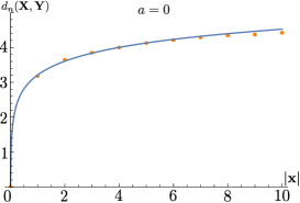
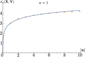
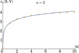
Figure 2: $d_{n}(\mathbf{X}_{a},\mathbf{Y}_{a})$ for $\beta_{a}=\exp(10.6-2.06a)$. $a=0,1,2$ from left to right. The solid line is the geodesic distance (3.17) with the fitted parameters.

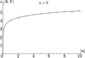
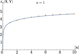
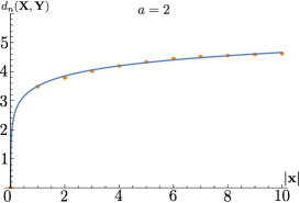
Figure 3: $d_{n}(\mathbf{X}_{a},\mathbf{Y}_{a})$ for $\beta_{a}=\exp[10.6-2.06a+(-1)^{a}]$. $a=0,1,2$ from left to right. The solid line is the geodesic distance (3.17) with the fitted parameters.

Using the obtained numerical results, we fit the parameters $\ell,\,\alpha,\,q$ in (3.15) by minimizing the following $\chi^{2}$:

$$\chi^{2}(\ell,\alpha,q)\equiv\sum_{\mathbf{x},a}\frac{\bigl{[}d_{n}\bigl{(}(\mathbf{x},\beta_{a}),(\mathbf{0},\beta_{a})\bigr{)}-\mathcal{I}(\mathbf{x},\beta_{a};\ell,\alpha,q)\bigr{]}^{2}}{\mbox{Var}\bigl{[}d_{n}\bigl{(}(\mathbf{x},\beta_{a}),(\mathbf{0},\beta_{a})\bigr{)}\bigr{]}}.$$ (3.18)

For the first choice (exponential form) we obtain $\ell=0.0445\pm 0.0002$, $\alpha=(1.180\pm 0.022)\times 10^{5}$, $q=0.313\pm 0.001$, with $\sqrt{\chi^{2}/30}=13.6$, and for the second choice (zigzag form) we obtain $\ell=0.0624\pm 0.0002$, $\alpha=(4.421\pm 0.165)\times 10^{5}$, $q=0.497\pm 0.002$, with $\sqrt{\chi^{2}/30}=6.9$. We draw the geodesic distances with these fitted parameters as solid lines in figs. 2 and 3. The good agreement shows that the distances can be regarded as geodesic distances of an asymptotically Euclidean AdS metric, and also that this conclusion does not depend on the choice of the functional form of $\beta_{a}$.

4 Optimization of the tempering parameter

In this section, we optimize the tempering parameter by demanding that the distances get minimized. We will show that a simple, geometrical consideration gives the conclusion that $\beta_{a}$’s take an exponential form for large $\beta_{a}$. We further will confirm this conclusion by numerically optimizing the tempering parameter set. We show that the optimized parameter set actually takes an exponential form for large $\beta_{a}$ and that they also exhibit a horizon for small $\beta_{a}$, beyond which configurations can move freely in the $x$ direction.

4.1 Need for the optimization of $\beta_{a}$

The tempering parameter set $\mathcal{A}=\{\beta_{a}\}$ must be chosen such that transitions in the $\beta$ direction have significant acceptance rates and also that transitions in the $x$ direction are easy for some $\beta_{a}$. If $\beta$ represents the overall coefficient of the action and we order $\mathcal{A}=\{\beta_{a}\}$ as $\beta_{0}>\beta_{1}>\cdots>\beta_{A}$ [as we have done for the action (2.9)], then the above requirement means that $\beta_{a}$ must be placed densely to some extent (and thus $A$ must be large), and also that $\beta_{a}$ $(a\sim A)$ must be sufficiently small such that severe potential barriers no longer exist there. However, if one introduced too many $\beta_{a}$’s, the size of the subsample with $\beta_{a=0}$ would become small and the sample average would get a large statistical error. This enforces us to make a careful adjustment of the elements of the set $\mathcal{A}=\{\beta_{a}\}$. We will show in the next subsection that this adjustment can be carried out in a simple, geometrical way.

4.2 Geometrical optimization of the tempering parameter

In section 3, we showed that the metric in the extended, coarse-grained configuration space has the component:

$$ds^{2}|_{x={\rm const}}=d_{n}^{2}\bigl{(}(x,\beta),(x,\beta+d\beta)\bigr{)}={\rm const.}\,\frac{d\beta^{2}}{\beta^{2}}={\rm const.}\,\Bigl{(}\frac{\beta^{\prime}(a)}{\beta(a)}\Bigr{)}^{2}\,da^{2},$$ (4.1)

where we regard $\beta(a)\equiv\beta_{a}$ as a continuous function of $a$. To accelerate the relaxation of the probability distribution, we need to optimize the tempering parameter set $\{\beta_{a}\}$. Since almost all of the transitions occur only in the $\beta$ direction for large $\beta_{a}$, the optimization should be made so that the transitions in the $\beta$ direction has no obstacle for large $\beta$. Since it is the parameter $a$ that is directly dealt with by a MCMC simulation, the above requirement can be re-expressed as a geometrical statement that the metric in the $a$ direction is flat. This means the equality

$$\frac{\beta^{\prime}(a)}{\beta(a)}={\rm const.},$$ (4.2)

and thus we conclude that the optimized tempering parameter set should have an exponential form, $\beta_{a}=\beta_{0}\,R^{-a}$ ($R$: constant). Note that this form is expected only for large $\beta_{a}$’s, because for small enough $\beta_{a}$, transitions in the $x$ direction come to occur frequently and thus the above argument no longer holds.

4.3 Numerical confirmation of the geometrical optimization

In this subsection, we numerically optimize the tempering parameter set $\{\beta_{a}\}$, and show that the optimized set actually takes an exponential form for large $\beta_{a}$. We also show that there exists a horizon for small $\beta_{a}$, beyond which configurations can move freely in the $x$ direction.

Below is the numerical algorithm we take to optimize the tempering parameter set. We here fix $\beta_{0}$ (the overall coefficient of the original action), $n$ (the number of steps), and $A$ (the number of the additional parameters), and vary the parameters $\bm{\beta}\equiv\{\beta_{a}\}_{a=1,\ldots,A}$ such that the distances between different modes $\mathbf{X}_{1}=(\mathbf{x}_{1},\beta_{0}),\,\mathbf{X}_{2}=(\mathbf{x}_{2},\beta_{0})\in\bar{\mathcal{M}}\times\mathcal{A}$ are minimized. For given initial parameters $\bm{\beta}$, we update them with the following steps:

1. We calculate the distance $d_{n}(\mathbf{X}_{1},\mathbf{X}_{2};\bm{\beta})$ for $\bm{\beta}$.

2. We propose a new parameter set $\bm{\beta}^{\prime}=\{\beta_{0},\ldots,\beta_{a-1},\beta_{a}^{\prime},\beta_{a+1},\ldots,\beta_{A}\}$ by generating $\ln{\beta_{a}^{\prime}}$ using the Gaussian distribution with mean $\ln\beta_{a}$ and standard deviation $\sigma_{\beta}$ (a constant given in advance) for randomly selected $a$. If the obtained parameters are not ordered, we repeatedly generate another set until we get ordered ones.

3. We calculate the distance $d_{n}(\mathbf{X}_{1},\mathbf{X}_{2};\bm{\beta}^{\prime})$ for the new parameter set, and update $\bm{\beta}$ to $\bm{\beta^{\prime}}$ if $d_{n}(\mathbf{X}_{1},\mathbf{X}_{2};\bm{\beta}^{\prime})<d_{n}(\mathbf{X}_{1},\mathbf{X}_{2};\bm{\beta})$.

4. We repeat steps 2 and 3. Since the calculated distance can be unintentionally small due to a statistical error, it can happen that we reject a set which should be accepted. To avoid this to happen frequently, we recalculate the distance with a larger precision when proposed sets are rejected $N_{\mathrm{discard}}$ times sequentially ($N_{\mathrm{discard}}$ is a number given in advance).

Figure 4 shows the optimized values of $\{\beta_{a}\}$ $(a=1,\ldots,A)$ for a 2-dimensional ($D=2$) noncompact configuration space with the parameters $k=8$ and $n=100$.

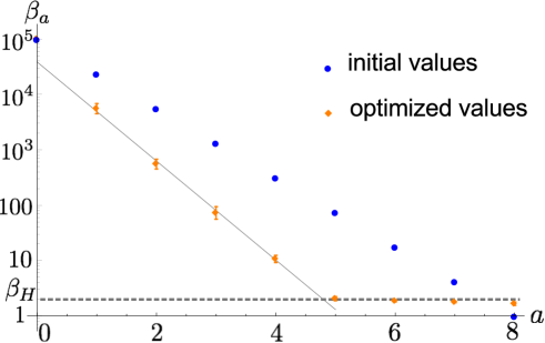
Figure 4: Optimized values for $\bm{\beta}=\{\beta_{a}\}$ $(a=1,\ldots,8)$. The blue dots are the initial values, and the orange dots give the resulting optimized values that minimize the distance $d_{n}(\mathbf{X}_{1},\mathbf{X}_{2})$. The horizontal dashed line at $\beta_{H}\simeq 2$ represents the horizon, beyond which configurations can move freely in the $x$ direction.

We set $\beta_{0}=10^{5}$, $A=8$, $\sigma_{\beta}=(\ln\beta_{0})/(4A)$ and $N_{\mathrm{discard}}=10$. We start from initial values $\beta_{a}=\beta_{0}^{1-a/A}$. We use the Metropolis algorithm to generate a transition in the $\mathbf{x}$ direction, using the Gaussian distribution with standard deviation $\sigma_{x}(\beta_{a})=1.6/(2\pi\sqrt{2\beta_{a}})$ as a proposal distribution. We calculate the distance $d_{n=100}(\mathbf{X}_{1},\mathbf{X}_{2};\bm{\beta})$ between $\mathbf{X}_{1}=((1,0),\beta_{0})$ and $\mathbf{X}_{2}=((0,0),\beta_{0})$ for given $\bm{\beta}$. We first repeat steps 2 and 3 10,000 times, where at least 100 paths from $\mathbf{X}_{1}$ to $\mathbf{X}_{2}$ are generated to calculate the distance. Following this, we then repeat the same procedures 15,000 times, but this time at least 200 paths are generated. After we obtain the optimized values (drawn as orange points in fig. 4), we fit the points in the region $1\leq a\leq 4$ with a linear function $c_{1}a+c_{2}$ by minimizing $\chi^{2}$. We obtain $c_{1}=-2.06\pm 0.08$, $c_{2}=10.6\pm 0.2$ with $\sqrt{\chi^{2}/4}=0.48$. The points near the boundary $a=0$ behaves differently which may be explained as boundary effects. We also see that $\beta_{a}$ $(a=5,6,7,8)$ have almost the same value, $\beta_{H}\sim 2$. $\beta_{H}$ represents a “horizon”, beyond which the potential barriers in the $x$ direction disappear and configurations can move freely in the direction. Thus, the value $A=8$ is actually too large, and we find that five parameters $\beta_{a}$ $(a=1,\ldots,5)$ should be enough for this calculation.

We thus arrive at the conclusion that the optimized tempering parameter is given by an exponential form, $\beta_{a}=\beta_{0}\,R^{-a}$, except for those near boundaries. This confirms the geometrical optimization made in subsection 4.2.

We end this subsection with a comment that there are actually many metastable solutions for $\bm{\beta}$ and all such solutions also take exponential forms. The left panel of fig. 5 is the history of $d_{n}^{2}(\mathbf{X}_{1},\mathbf{X}_{2};\bm{\beta})$ with respect to the updates of $\bm{\beta}$.

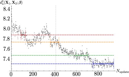
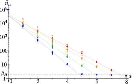
Figure 5: (Left) History of $d_{n}^{2}(\mathbf{X}_{1},\mathbf{X}_{2};\bm{\beta})$ with respect to the updates of $\bm{\beta}$. Smaller $\sigma_{\beta}$ is used for step 3 after the number of updates of $\bm{\beta}$ exceeds 410. (Right) Metastable solutions. Each solid line represents a metastable solution $\bm{\beta}=\{\beta_{a}\}$ defined as the average of the values of $\bm{\beta}$’s belonging to a segment drawn in the left panel.

We there see several plateaus that correspond to metastable states. The right panel shows that the metastable solutions, each corresponding to a plateau, actually take exponential forms.

5 Conclusion and outlook

In this paper, we have investigated the global geometry of a stochastic system whose equilibrium distribution is highly multimodal with a large number of degenerate vacua that are distributed uniformly.

We implemented the simulated tempering algorithm to such a system by taking the tempering parameter to be the overall coefficient $\beta_{0}$ of the action. We showed that the geometry of the extended, coarse-grained configuration space $\bar{\mathcal{M}}\times\mathcal{A}$ is given by an asymptotically AdS space. With this knowledge of geometry, we deduced the conclusion that the optimized tempering parameter set $\{\beta_{a}\}$ must take an exponential form $\beta_{a}=\beta_{0}\,R^{-a}$ for large $\beta_{a}$. This conclusion was confirmed by numerical calculations, where it was also found that a horizon exists at small $\beta$, around which transitions in the $x$ direction become easy.

As for the future work, it would be interesting to investigate the large scale geometry of the configuration space in the Yang-Mills theory, especially by coarse-graining the configuration space according to the topological charges.

It should also be important to construct a more convenient method to find the optimized parameters for a given MCMC algorithm. For the simulated tempering algorithm, for example, the optimization is to determine the functional form of $\beta_{a}=\beta(a)$. Thus, it should be nice if we can find a local functional of $\beta(a)$ such that the optimized form is directly given by solving its Euler-Lagrange equation, and further if this local functional has some relationship with the Einstein-Hilbert action. We expect that this investigation may also give a clue to understanding the hidden stochastic character in general relativity.

In this paper, we have discussed only the case where the action $S(x)$ is real. When the action takes complex values as in QCD at finite density or in the quantum Monte Carlo computation of the Hubbard model away from half filling, we cannot directly use the present definition of distance because the Boltzmann weight is complex-valued. It must be important to investigate whether nice distances can also be introduced to these algorithms. In particular, it must be interesting to investigate the large scale geometry of the (generalized) Lefschetz thimble method [8, 9, 10, 11, 12, 13, 14, 15] with the implementation of the tempering algorithm that takes the tempering parameter to be the flow time of the antiholomorphic gradient flow [14, 15].

A study along these lines is now in progress and will be reported elsewhere.

Appendix A Triangle inequality on the extended, coarse-grained configuration space

We demonstrate that the distance $d_{n}(X,Y)$ satisfies the triangle inequality also in the extended, coarse-grained configuration space $\bar{\mathcal{M}}\times\mathcal{A}$ for $\beta_{a}\gg 1$.

For this purpose, we explicitly calculate the value $d_{n}(X,Y)+d_{n}(Y,Z)-d_{n}(X,Z)$ by taking three points $X,Y,Z\in\bar{\mathcal{M}}\times\mathcal{A}$ in various ways. We use the action (2.9) with parameters $D=2$ and $L=100$. The tempering parameter is set to $\beta_{a}=100\cdot 10^{-3a/10}$ ($a=-200,\ldots,200$). To generate a transition in the $\mathbf{x}$ direction, we use the same Metropolis algorithm but now set the standard deviation of the Gaussian proposal distribution to $\sigma_{x}(\beta_{a})=1.6/(2\pi\sqrt{2\beta_{a}})$. We set $k=8$ and $n=1,000$, and generate $10^{6}$ configurations from each initial configuration. In table 1, we show the result for $X=((0,0),\beta_{0})$, $Y=((y,0),\beta_{a})$ and $Z=((3,0),\beta_{1})$ with $y=0,\ldots,6$ and $a=-2,\ldots,2$.

$a$ \ $y$	0	1	2	3	4	5	6
-2	0.0$\pm$1.2	1.4$\pm$0.1	2.3$\pm$0.1	0.1$\pm$1.0	2.7$\pm$0.1	3.1$\pm$0.1	3.5$\pm$0.1
-1	0.1$\pm$0.2	2.3$\pm$0.1	2.3$\pm$0.1	0.2$\pm$0.1	2.6$\pm$0.1	3.2$\pm$0.1	3.5$\pm$0.1
0	0.0$\pm$0.1	2.2$\pm$0.1	2.2$\pm$0.1	0.2$\pm$0.2	2.7$\pm$0.1	3.3$\pm$0.2	3.4$\pm$0.1
1	0.1$\pm$0.2	2.1$\pm$0.1	2.1$\pm$0.1	0.0$\pm$0.1	2.5$\pm$0.1	3.0$\pm$0.1	3.4$\pm$0.2
2	0.11$\pm$0.16	2.1$\pm$0.1	2.1$\pm$0.1	0.13$\pm$0.15	2.4$\pm$0.1	3.0$\pm$0.1	3.3$\pm 0.1$

Table 1: $d_{n}(X,Y)+d_{n}(Y,Z)-d_{n}(X,Z)$ for $X=((0,0),\beta_{0})$, $Y=((y,0),\beta_{a})$ and $Z=((3,0),\beta_{1})$. $\beta_{a}$ are set to $\beta_{-2}\simeq 400$, $\beta_{-1}\simeq 200$, $\beta_{0}=100$, $\beta_{1}\simeq 50$, $\beta_{2}\simeq 25$. All the entries are positive within statistical errors, which shows that the triangle inequality holds.

We see that $d_{n}(X,Y)$ does satisfy the triangle inequality on $\bar{\mathcal{M}}\times\mathcal{A}$.

Appendix B Calculation of eq. (3.2)

In this appendix, we evaluate the integral that appears in (3.2):

$$I\equiv\int_{\mathcal{M}}d^{D}x\,\min\Bigl{(}1,\frac{P_{\mathrm{eq}}(\mathbf{x},\beta_{b})}{P_{\mathrm{eq}}(\mathbf{x},\beta_{a})}\Bigr{)}\,P_{\mathrm{eq}}^{(\mathrm{loc})}(\mathbf{x},\beta_{a}).$$ (B.1)

We are concerned with the case where $\beta_{a},\,\beta_{b}\gg 1$, and thus can approximate $P_{\mathrm{eq}}(\mathbf{x},\beta_{a})$ by the Gaussian distributions around local minima [see (3.6)]. Due to the translational invariance, we only need to consider the local minimum at the origin, for which the integrand becomes

$$\min\Big{(}(2\pi\beta_{a})^{D/2}\,e^{-2\pi^{2}\beta_{a}r^{2}},(2\pi\beta_{b})^{D/2}\,e^{-2\pi^{2}\beta_{b}r^{2}}\Big{)}\quad(r^{2}\equiv\mathbf{x}^{2}).$$ (B.2)

Let us first consider the case $\beta_{a}<\beta_{b}$.

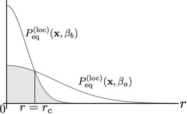
Figure 6: The integrand (B.2) for the case $\beta_{a}<\beta_{b}$. The integral (B.1) is given by the volume of the shaded region.

The integral of (B.2) then can be evaluated as (see Fig. 6)

$$I \simeq\Omega_{D-1}\,\bigg{[}\int_{0}^{r_{c}}dr\ r^{D-1}(2\pi\beta_{a})^{D/2}\,e^{-2\pi^{2}\beta_{a}r^{2}}+\int_{r_{c}}^{\infty}dr\ r^{D-1}(2\pi\beta_{b})^{D/2}\,e^{-2\pi^{2}\beta_{b}r^{2}}\bigg{]}$$

$$=1-\Omega_{D-1}\,\bigg{[}-(2\pi\beta_{a})^{D/2}\int_{0}^{r_{c}}dr\ r^{D-1}\,e^{-2\pi^{2}\beta_{a}r^{2}}+(2\pi\beta_{b})^{D/2}\int_{0}^{r_{c}}dr\ r^{D-1}e^{-2\pi^{2}\beta_{b}r^{2}}\bigg{]},$$ (B.3)

where $\Omega_{D-1}=2\pi^{D/2}/\Gamma(D/2)$ is the volume of $(D-1)$-sphere, and $r_{c}$ is defined by

$$r_{c}\equiv\sqrt{\frac{(D/2)\ln(\beta_{b}/\beta_{a})}{2\pi^{2}(\beta_{b}-\beta_{a})}}.$$ (B.4)

The remaining integral in (B.3) can be written in terms of the lower incomplete gamma function $\gamma(z,p)=\int_{0}^{p}dt\,e^{-t}\,t^{z-1}$ as

$$I \simeq 1-\frac{1}{\Gamma(D/2)}\,\big{[}-\gamma(D/2,{\tilde{r}_{c}}^{2})+\gamma(D/2,{\tilde{s}_{c}}^{2})\big{]},$$ (B.5)

where ${\tilde{r}_{c}}$ and ${\tilde{s}_{c}}$ are defined by

$$\tilde{r}_{c} \equiv r_{c}\sqrt{2\pi^{2}\beta_{a}}=\sqrt{2\pi^{2}\frac{(D/2)\ln(\beta_{b}/\beta_{a})}{2\pi^{2}(\beta_{b}/\beta_{a}-1)}},$$

$$\tilde{s}_{c} \equiv r_{c}\sqrt{2\pi^{2}\beta_{b}}=\sqrt{2\pi^{2}\frac{(D/2)\ln(\beta_{b}/\beta_{a})}{2\pi^{2}(1-\beta_{a}/\beta_{b})}},$$ (B.6)

and depend on $\beta_{a},\,\beta_{b}$ only through the ratio $\beta_{b}/\beta_{a}$. The integral $I$ for the case $\beta_{a}>\beta_{b}$ can also be evaluated in the same way. We thus obtain

$$I\simeq 1-\frac{1}{\Gamma(D/2)}\,\bigl{|}\gamma(D/2,{\tilde{r}_{c}}^{2})-\gamma(D/2,{\tilde{s}_{c}}^{2})\bigr{|}\equiv 1-\Delta(\beta_{b}/\beta_{a}),$$ (B.7)

which is actually an expression valid for the both cases, $\beta_{a}\lessgtr\beta_{b}$.

References

- [1] M. Fukuma, N. Matsumoto and N. Umeda, “Distance between configurations in Markov chain Monte Carlo simulations,” JHEP 1712, 001 (2017) [arXiv:1705.06097 [hep-lat]].
- [2] M. Creutz, “Overrelaxation and Monte Carlo Simulation,” Phys. Rev. D 36, 515 (1987).
- [3] E. Marinari and G. Parisi, “Simulated tempering: A New Monte Carlo scheme,” Europhys. Lett. 19, 451 (1992) [hep-lat/9205018].
- [4] R. H. Swendsen and J.-S. Wang, “Replica Monte Carlo Simulation of Spin-Glasses,” Phys. Rev. Lett. 57 2607 (1986).
- [5] C. J. Geyer, “Markov Chain Monte Carlo Maximum Likelihood,” in Computing Science and Statistics: Proceedings of the 23rd Symposium on the Interface, American Statistical Association, New York, p. 156 (1991).
- [6] D. J. Earl and M. W. Deem, “Parallel tempering: Theory, applications, and new perspectives,” Phys. Chem. Chem. Phys. 7, 3910 (2005).
- [7] M. Lüscher, JHEP 1008, 071 (2010) Erratum: [JHEP 1403, 092 (2014)] doi:10.1007/JHEP08(2010)071, 10.1007/JHEP03(2014)092 [arXiv:1006.4518 [hep-lat]].
- [8] M. Cristoforetti, F. Di Renzo and L. Scorzato, “New approach to the sign problem in quantum field theories: High density QCD on a Lefschetz thimble,” Phys. Rev. D 86, 074506 (2012) [arXiv:1205.3996 [hep-lat]].
- [9] M. Cristoforetti, F. Di Renzo, A. Mukherjee and L. Scorzato, “Monte Carlo simulations on the Lefschetz thimble: Taming the sign problem,” Phys. Rev. D 88, no. 5, 051501 (2013) [arXiv:1303.7204 [hep-lat]].
- [10] A. Mukherjee, M. Cristoforetti and L. Scorzato, “Metropolis Monte Carlo integration on the Lefschetz thimble: Application to a one-plaquette model,” Phys. Rev. D 88, no. 5, 051502 (2013) [arXiv:1308.0233 [physics.comp-ph]].
- [11] H. Fujii, D. Honda, M. Kato, Y. Kikukawa, S. Komatsu and T. Sano, “Hybrid Monte Carlo on Lefschetz thimbles - A study of the residual sign problem,” JHEP 1310, 147 (2013) [arXiv:1309.4371 [hep-lat]].
- [12] M. Cristoforetti, F. Di Renzo, G. Eruzzi, A. Mukherjee, C. Schmidt, L. Scorzato and C. Torrero, “An efficient method to compute the residual phase on a Lefschetz thimble,” Phys. Rev. D 89, no. 11, 114505 (2014) [arXiv:1403.5637 [hep-lat]].
- [13] A. Alexandru, G. Başar, P. F. Bedaque, G. W. Ridgway and N. C. Warrington, “Sign problem and Monte Carlo calculations beyond Lefschetz thimbles,” JHEP 1605, 053 (2016) [arXiv:1512.08764 [hep-lat]].
- [14] M. Fukuma and N. Umeda, “Parallel tempering algorithm for integration over Lefschetz thimbles,” PTEP 2017, no. 7, 073B01 (2017) [arXiv:1703.00861 [hep-lat]].
- [15] A. Alexandru, G. Başar, P. F. Bedaque and N. C. Warrington, “Tempered transitions between thimbles,” Phys. Rev. D 96, no. 3, 034513 (2017) [arXiv:1703.02414 [hep-lat]].