Solitary waves in the Ablowitz–Ladik equation with power-law nonlinearity

Abstract

We introduce a generalized version of the Ablowitz-Ladik model with a power-law nonlinearity, as a discretization of the continuum nonlinear Schrödinger equation with the same type of the nonlinearity. The model opens a way to study the interplay of discreteness and nonlinearity features. We identify stationary discrete-soliton states for different values of nonlinearity power $\sigma$, and address changes of their stability as frequency $\omega$ of the standing wave varies for given $\sigma$. Along with numerical methods, a variational approximation is used to predict the form of the discrete solitons, their stability changes, and bistability features by means of the Vakhitov-Kolokolov criterion (developed from the first principles). Development of instabilities and the resulting asymptotic dynamics are explored by means of direct simulations.

I Introduction

The study of models of the discrete nonlinear-Schrödinger (DNLS) type has been a focal point within the broader theme of nonlinear dynamical lattices over the past two decades book . First, DNLS systems are obviously relevant to the discretization of the ubiquitous continuum nonlinear Schrödinger equations sulem ; ablowitz ; ussiam . Still more important is, arguably, the relevance of DNLS equations in their own right as physical models in a multitude of settings. In particular, they have been extensively used for modeling light propagation in arrays of optical waveguides dnc ; moti . They have been also greatly employed for the development of the broad topic of dynamics of atomic Bose-Einstein condensates (BECs) trapped in deep optical lattices ober . Other important applications of DNLS models are the study of the denaturation of the  DNA double strand Peybi , breathers in granular crystals chong , the dynamics of protein loops niemi , etc.

A model that plays a critical role in the understanding of DNLS dynamical lattices is their integrable sibling, namely, the Ablowitz-Ladik (AL) equation ablolad (see also ablowitz ). In addition to offering the unique integrability structure ablowitz , the AL model is a reference point for the examination of numerous features of nonlinear discrete settings, such as stability of solitary waves kapitula , Bloch oscillations bishop , etc. The AL equation is also important as an ingredient of the Salerno model, which combines it with the nonintegrable DNLS equation salerno . The Salerno model was widely used, as a platform for developing perturbation theory and exploring direct numerical simulations cai , in various contexts, including, in particular, the challenging problem of collisions between solitary waves in dynamical lattices dmitriev . Further, the AL equation by itself, and in the form of its Salerno generalization, provides for the mean-field limit of the class of quantum systems in the form of the so-called “nonstandard” Bose-Hubbard lattices (BHLs), in which the inter-site coupling depends on the sites’ populations (hence the coupling is nonlinear, in terms of the mean-field approximation). Numerous realizations of such BHLs, including their mean-field realizations, were reviewed in a recent survey article review . Actually, the list of applications of the AL model is anything but exhaustive, as relevant applications continue to emerge through the examination, e.g. more recently, of features such as rogue waves in the AL model akhm ; yang , and their comparison to the DNLS case hoffman .

In the present work, we consider a variant of the AL model with a power-law nonlinearity instead of the particular case of the cubic one. This is motivated by many previous studies —see e.g. sulem and references therein for the continuum case, as well as Refs.  Turitsyn ; malomed ; weinstein ; ourDNLS ; Kladko for the discrete case— of the generalized NLS model with nonlinear term $|\psi|^{2\sigma}\psi$ instead of the usual cubic one corresponding to the particular value of $\sigma=1$. In particular, in the one-dimensional (1D) case the Lee-Huang-Yang correction to the mean-field nonlinearity in two-component Bose-Einstein condensates (BECs) corresponds to the self-attractive term with $\sigma=0.5$ Grisha1 ; Grisha2 . The model with a general nonlinear term is particularly appealing because it offers, at the continuum level and for one spatial dimension, the potential to study the transition from integrability (at $\sigma=1$) and the existence of stable solitary waves (at $\sigma<2$) to the emergence of catastrophic self-focusing (at $\sigma\geq 2$). In the DNLS variant of the model, there exist interesting features too, such as bistability (for a range of values of $\sigma$), as well as the emergence of energy thresholds for the existence of discrete solitons, again for $\sigma>2$ in one spatial dimension. However, the AL generalization to a power-law nonlinearity was not explored before, to the best of our knowledge. It is the aim of the present work to report this analysis.

More specifically, our aim is to examine the nature of discrete solitons for the AL-type lattice nonlinearity, $\propto|\psi_{n}|^{2\sigma}(\psi_{n+1}+\psi_{n-1})$, with different values of $\sigma$ (characterizing also the structure of these discrete solitons by means of a variational approach) and to explore whether these modes change their stability with the variation of their intrinsic frequency (alias chemical potential, in terms of BEC) for given $\sigma$. In particular, we aim to find out if the stability change can be predicted by a variant of the Vakhitov-Kolokolov (VK) criterion, which is well known in other contexts Vakh ; book — In the DNLS (and NLS) settings, the VK criterion suggests that a change of the monotonicity of the $l^{2}$ (or $L^{2}$, respectively) norm vs. the soliton’s intrinsic frequency dependence induces a change of its stability book .Finally, we explore the full stability (via the spectral stability analysis) and evolution of instabilities in the model, by means of numerical computations. This allows us, among other features, to corroborate predictions of the VK criterion and analyze manifestations of the bistability in the model.

Our presentation is structured as follows. In section II, we offer our analytical considerations, including the model setup, the present variant of the VK criterion, and the variational approximation. In section III, we show numerical computations concerning both the existence and spectral stability of discrete solitons and their nonlinear evolution. Finally, in section IV we summarize our findings and discuss directions for further work.

II Analytical Considerations

II.1 The general Setup, conservation laws, and stability analysis

Our generalized AL model with the power-law nonlinearity is introduced as

$$\mathrm{i}\dot{\psi}_{n}+C(\psi_{n+1}+\psi_{n-1})+\beta(\psi_{n+1}+\psi_{n-1})|\psi_{n}|^{2\sigma}=0.$$ (1)

Here, $C$ is the (linear) coupling constant between adjacent sites, while $\sigma$ represents, as defined above, the nonlinearity power. In what follows below, we fix $\beta=1$ by means of obvious rescaling, considering the focusing sign of the nonlinearity ($\beta>0$). This model can be thought of as a discretization of the NLS model with the general power-law nonlinearity sulem . At the same time, as mentioned above, it is an intriguing setup for exploring differences (for sufficiently large $\sigma$, such as $\sigma>2$ in the 1D case considered here) of the collapse phenomenology in discrete vs. continuum models. With these motivations in mind, we will construct localized states of the model, investigate their stability through computation of eigenvalues of small perturbations, and numerically examine evolution of unstable states.

An important property of Eq. (1) is that it preserves a suitably defined norm-like quantity. The derivation of this property, that we will develop here, is generally applicable to nonlinear lattice equations of the form

$$\mathrm{i}\dot{\psi}_{n}+(C+f(|\psi_{n}|^{2}))(\psi_{n+1}+\psi_{n-1})=0,$$ (2)

where $f$ may be an arbitrary real function of $|\psi_{n}|^{2}$. We assuming that $P$ (which should revert to the usual $L^{2}$ norm in the continuum limit) depends only on the on-site intensity $|\psi_{n}|^{2}$:

$$P=\sum_{n}g(|\psi_{n}|^{2}).$$ (3)

From here it follows that

$$\mathrm{i}\frac{dP}{dt}=\sum_{n}g^{\prime}(C+f)\left[\left(\psi_{n+1}^{\star}\psi_{n}-\psi_{n+1}\psi_{n}^{\star}\right)-\left(\psi_{n}^{\star}\psi_{n-1}-\psi_{n}\psi_{n-1}^{\star}\right)\right],$$ (4)

where Eq. (1) is used to substitute $d\psi_{n}/dt$, and $g^{\prime}$ stands for the derivative of $g$. Thus, the selection of $g^{\prime}=1/(C+f)$ leads $dP/dt=0$, due to the telescopic nature of the resulting summation. For the particular case of $f(x)=x^{\sigma}$, this results in

$$P=\frac{1}{C}\sum_{n}|\psi_{n}|^{2}{}_{2}F_{1}\left(1,1/\sigma;1+1/\sigma;-\frac{|\psi_{n}|^{2\sigma}}{C}\right)\equiv\sum_{n}\mathcal{P}_{n},$$ (5)

where $\mathcal{P}_{n}$ is the density associated with the conserved quantity at each node, and ${}_{2}F_{1}$ is the Gauss hypergeometric function. In the special case of $\sigma=1$, it is straightforward to see that this falls back to the simple expression relevant for the cubic integrable AL model cai , $\left(\mathcal{P}_{n}\right)_{\sigma=1}=\ln\left(1+\frac{1}{C}\left|\psi_{n}\right|^{2}\right)$ (up to a $C$-dependent constant prefactor). We have thus obtained an important, even if somewhat cumbersome, conservation law for Eq. (1).

A further important observation for Eq. (1) is that a natural way to analyze the system can be to explore its similarity to the integrable case of $\sigma=1$ and the perturbation theory around it cai ; review . In particular, we conclude that the Hamiltonian of the general AL equation remains the same as in the integrable case,

$$H=-\sum_{n}\left(\psi_{n}\psi_{n+1}^{\star}+\psi_{n}^{\star}\psi_{n+1}\right),$$ (6)

being a conserved quantity too. It is also relevant to define the Poisson brackets corresponding to this Hamiltonian:

$$\{B,\tilde{B}\}=\mathrm{i}\sum_{n}\left(\frac{\partial B}{\partial\psi_{n}}\frac{\partial\tilde{B}}{\partial\psi_{n}^{\star}}-\frac{\partial B}{\partial\psi_{n}^{\star}}\frac{\partial\tilde{B}}{\partial\psi_{n}}\right)(C+f),$$ (7)

where $B$ and $\tilde{B}$ are two arbitrary functionals. This definition leads to $\{\psi_{n},\psi_{m}^{\star}\}=i(C+f)\delta_{nm}$, while $\{\psi_{n}\psi_{m}\}=\{\psi_{n}^{\star},\psi_{m}^{\star}\}=0$. The respective Hamiltonian form of Eq. (2) is

$$\dot{\psi}_{n}=\{H,\psi_{n}\}.$$ (8)

In our numerical computations, we sought for stationary solutions with frequency $-\omega$, in the form of $\psi_{n}(t)=\phi_{n}\mathrm{e}^{\mathrm{i}(\omega+2C)t}$ with real $\phi_{n}$ obeying the following set of algebraic equations:

$$-\omega\phi_{n}+C(\phi_{n+1}+\phi_{n-1}-2\phi_{n})+(\phi_{n+1}+\phi_{n-1})\phi_{n}^{2\sigma}=0.$$ (9)

The linear stability was explored by considering perturbations with infinitesimal amplitude $\delta$ around the stationary solutions. To this end, we substitute ansatz $\psi_{n}(t)=\mathrm{e}^{i(\omega+2C)t}\left[\phi_{n}+\delta(a_{n}\mathrm{e}^{\lambda t}+b_{n}^{\ast}\mathrm{e}^{\lambda^{\ast}t})\right]$ in Eq. (9), and then solve the ensuing linearized eigenvalue problem: $\lambda(a_{n},b_{n})^{T}=\mathcal{M}(a_{n},b_{n})^{T}$, with matrix

$$\mathcal{M}=\mathrm{i}\left(\begin{array}[]{cc}L_{1}&L_{2}\\ &\\ -L_{2}^{\ast}&-L_{1}^{\ast}\end{array}\right),$$ (10)

where submatrices $L_{1}$ and $L_{2}$ in Eq. (10) are composed of the following entries:

$$(L_{1})_{n,m}=\left[-\omega-2C+\sigma(\phi_{n+1}+\phi_{n-1})\phi_{n}^{2\sigma-2}\phi_{n}\right]\delta_{n,m}+(C+\phi_{n}^{2\sigma})(\delta_{n,m+1}+\delta_{n,m-1}),$$ (11)

$$(L_{2})_{n,m}=\sigma(\phi_{n+1}+\phi_{n-1})\phi_{n}^{2\sigma-1}\delta_{n,m}$$ (12)

The stationary solutions are spectrally stable if the eigenvalue problem produces purely imaginary $\lambda$. On the contrary, the existence of eigenvalues with nonzero real parts implies instability. In the latter case, it is of particular interest to simulate nonlinear evolution of unstable states.

II.2 The stationary variational approximation

Before turning to numerical computations, it is natural to apply a variational approximation (VA) progopt to the stationary equation (9). This will allow us to examine how well numerical solutions, that are produced in the next section, can be approximated by the simple (exponentially decaying) analytical expressions. To this end, we define

$$\phi_{n}\equiv C^{1/\left(2\sigma\right)}\chi_{n}~{},~{}~{}\frac{\omega}{C}\equiv\Omega,$$ (13)

and thus rewrite Eq. (9) as

$$(\chi_{n+1}+\chi_{n-1})-\frac{\left(2+\Omega\right)\chi_{n}}{1+\chi_{n}^{2\sigma}}=0,$$ (14)

which may generate bright solitons for $\Omega>0$.

The Lagrangian from which Eq. (14) can be derived is

$$L=\sum_{n=-\infty}^{+\infty}\left[\chi_{n+1}\chi_{n}-\left(2+\Omega\right)\int\frac{\chi_{n}d\chi_{n}}{1+\chi_{n}^{2\sigma}}\right]~{}.$$ (15)

The integral in this expression can be formally expressed in terms of the hypergeometric function, similar to Eq. (5), but such a formula is not really needed.

The simplest ansatz for the stationary soliton follows the pattern of Ref. malomed :

$$\chi_{n}=A\exp\left(-a|n|\right),$$ (16)

with $a>0$. Then, the first term in Eq. (15) is easily calculated, following the substitution of ansatz (16):

$$\sum_{n=-\infty}^{+\infty}\chi_{n+1}\chi_{n}=\frac{A^{2}}{\sinh a}.$$ (17)

The variational (Euler-Lagrange) equations intended to provide stationary discrete solitons solutions, derived from Lagrangian (15), in which ansatz (16) is substituted, read:

$$\frac{\partial L}{\partial A}=\frac{\partial L}{\partial a}=0.$$ (18)

The explicit form of the resulting equations is:

$$\frac{2}{\sinh a}-\left(2+\Omega\right)\sum_{n=-\infty}^{+\infty}\frac{\exp\left(-2a|n|\right)}{1+A^{2\sigma}\exp\left(-2\sigma a|n|\right)} = 0,$$ (19)

$$\frac{\cosh a}{\sinh^{2}a}-\left(2+\Omega\right)\sum_{n=-\infty}^{+\infty}\frac{|n|\exp\left(-2a|n|\right)}{1+A^{2\sigma}\exp\left(-2\sigma a|n|\right)} = 0.$$ (20)

The system of Eqs. (19) and (20) can be solved numerically for variable $A$ and $a$ if $\Omega>0$ and $\sigma$ are given. Although the solution of this system is still performed numerically, hence our approach is not fully analytical, the VA provides a significant insight into the problem, as it converts the infinite-dimensional original system into a much simpler system of two equations (19) and (20) for $A$ and $a$.

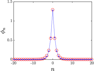
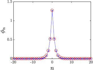
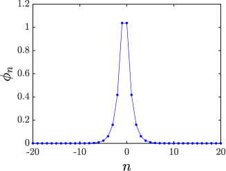
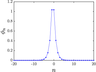
Figure 1: (Top panels) Exact numerically demonstrated profiles of the discrete soliton (blue lines and dots), and their counterparts predicted by the variational approximation (red circles), for 1-site solutions with $\omega=1$ and $C=1$. The displayed solutions are characterized by the respective values of $\sigma$, namely $\sigma=1.7$ (left), $\sigma=1.75$ (center) and $\sigma=2$ (right). (Bottom panels) Numerical profiles of discrete 2-site solitons with the same parameters of the 1-site soliton above.

III Numerical Results

First of all, we consider the dependence of the stability of 1-site (site-centered) and 2-site (inter-site centered) discrete solitons on the nonlinearity power $\sigma$ for fixed frequency $\omega=1$ and coupling $C=1$. Such solutions, e.g., for both kinds of modes at $\sigma=1.7$, $\sigma=1.75$ and $\sigma=2$ are depicted in Fig. 1. 1-site solitons are compared therein with profiles predicted by the VA, demonstrating close agreement between the two; while the VA is formulated for 1-site solitons, the numerical profiles of the inter-site centered counterparts are also given for completeness.

As it is well known book , in the case of the cubic ($\sigma=1$) AL equation, there are two eigenvalue pairs at zero, as a consequence of the translational and phase (gauge) invariance of the model. One of these invariances, namely the effective translational invariance, is broken in the non-integrable case, $\sigma\neq 1$. We start by analyzing the situation for $\sigma>1$. For 1-site solitons, computations demonstrate that the eigenvalue corresponding to the translational mode moves along the imaginary axis, whereas, at the same time, another mode departs from the linear-mode band; at $\sigma=\sigma_{c}$ (with $\sigma_{c}=1.674$ for the particular value of $C=1$), the latter mode becomes associated with a real eigenvalue pair, hence the 1-site solitons are unstable at $\sigma>\sigma_{c}$. For 2-site solitons, the translational mode moves along the real axis immediately beyond the integrable limit, consequently the relevant solutions are unstable for every $\sigma>1$. The scenario is quite different for $\sigma<1$, where the situation is reversed for 1-site and 2-site modes. In particular, in that case, the translational mode moves along the real (imaginary) axis for the 1-site (2-site) soliton, giving rise to exchange of the stability between them. It is worthy to note that a second stability exchange occurs at $\sigma=\sigma_{t}$, with $\sigma_{t}=0.5$ for all values of $C$ (recall that $\sigma=0.5$ corresponds to the LHY nonlinearity in the two-component BEC Grisha1 ). All these phenomena are summarized in Fig. 2.

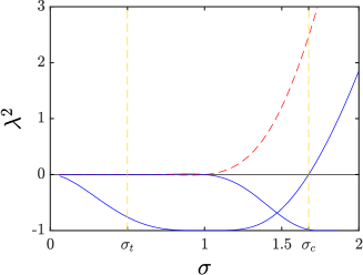
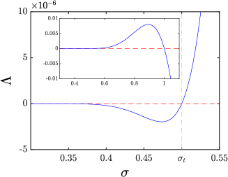
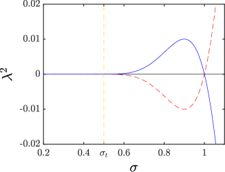
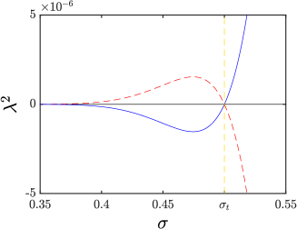
Figure 2: Top left panel: linear stability eigenvalues for 1-site (full blue line) and 2-site (dashed red line) discrete solitons as a function of $\sigma$ for $\omega=C=1$; top right panel: the dependence of the Hessian eigenvalue $\Lambda$ closest to zero for 1-site solitons with the same parameters set. Bottom panels provide zoom around points $\sigma=1$ (left panel) and $\sigma=0.5$ (right panel) of the top left panel, illustrating two stability exchanges occurring between the 1- and 2-site modes in the present model. The critical values of $\sigma$ for which the main bifurcations take place, namely $\sigma_{c}=1.674$ and $\sigma_{t}=0.5$ are highlighted by means of vertical dashed lines.

Secondly, we have analyzed the effect of varying the coupling constant on the critical values $\sigma_{c}$ and $\sigma_{t}$. The approach helps to reach the continuum limit, $C\rightarrow\infty$. Figure 3 shows the dependence of $\sigma_{c}$ on $C$ for $\omega=1$. One can observe that the minimum value of $\sigma_{c}$ is $\approx 1.669$, a value that is attained at $C\approx 1.16$; furthermore, $\sigma_{c}$ tends to $2$ when $C\rightarrow 0$ and $C\rightarrow\infty$. The latter retrieves the well-known continuum limit of the corresponding eigenvalue bifurcation towards the collapse sulem . As mentioned in the above paragraph, the critical value $\sigma_{t}$ is independent of $C$ and is equal to $1/2$. Interestingly, the spectrum of solitons for $\sigma=\sigma_{t}=0.5$ is the same as in the integrable Ablowitz-Ladik lattice $\sigma=1$ except for the occurrence of two (pairs of) localized eigenmodes, one at the top and another one at the bottom of the linear modes band. Notice that both 1-site and 2-site solitons possess the same spectrum,as illustrated in Fig. 4, and an associated neutral mode, as confirmed in Fig. 2. Notice, however, that the system in this case is not translationally invariant as the eigenvector that corresponds to the neutral mode (see right panel of the same figure) is not fully anti-symmetric, as is the case in the cubic ($\sigma=1$) limit.

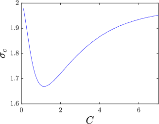
Figure 3: The dependence of critical value $\sigma_{c}$ on $C$ for $\omega=1$.

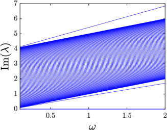
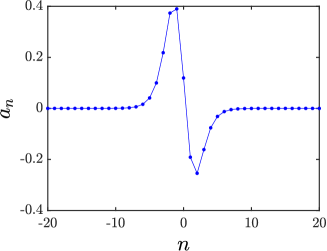
Figure 4: (Left panel) The dependence of the imaginary part of the stability eigenvalues for both 1-site and 2-site solitons with $C=1$ and $\sigma=\sigma_{t}=0.5$ with respect to $\omega$. (Right panel) 0-eigenmode for the 1-site soliton with $\sigma=0.5$ and $C=\omega=1$

Next we test the validity of the VK criterion in the present setting (see, e.g., book for its application to DNLS equations). It suggests that the change of monotonicity of the frequency dependence of the norm-like conserved quantity, defined as per Eq. (5) amounts to a change of stability. To examine this, we take 1-site solitons and vary $\omega$, fixing, e.g., $\sigma=1.7$ and $C=1$. The result is shown in Fig. 5, where one can indeed see the direct correlation between the slope of $P(\omega)$ dependence and the actual stability, as expected from the VK criterion, and from the general Grillakis-Shatah-Straus theory grillakis ; see Ref. kapprom for a recent overview. More specifically, the discrete solitons are found to be stable (unstable) when the slope is positive (negative). Additionally, in the case in which the emergence of an unstable linearization eigenvalue is not associated with a change of slope of the $P(\omega)$ curve one can compute the spectrum of the Hessian of the Hamiltonian (6) which can predict the existence of bifurcations through an eigenvalue zero crossing; this fact was illustrated in Fig. 2.

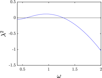
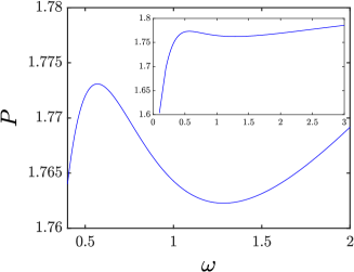
Figure 5: Dependences of the square of the relevant stability eigenvalue, $\lambda^{2}$, and conserved quantity $P$ on frequency $\omega$ (left and right panels, respectively) for 1-site solitons with $C=1$ and $\sigma=1.7$. The soliton is unstable in the interval of $\omega\in(0.56,1.29)$. Inset in right panel depicts the range $\omega\in(0,3]$ confirming the existence of only two extrema in the $P(\omega)$ curve.

We have also compared the predictions of the VA, presented in subsection II.2, with the results stemming from numerically exact (up to a prescribed accuracy) calculations for the discrete solitons. Figure 6 shows the amplitude, $\phi_{0}$, and the conserved quantity $P$ of 1-site solitons versus $\omega$, for three selected values of the nonlinearity power, $\sigma$ (namely, $\sigma=1.7$, $1.75$ and $2$) at fixed $C=1$; for other values of $C$, the VA predictions can be obtained by the rescaling defined in Eq. (13). Note that, as seen in Fig. 6, the VA predicts quite accurately the amplitude of the discrete soliton in all the cases considered, but there are some discrepancies in the dependence of the conserved quantity $P$. In any case, the VA approach is more accurate for higher frequencies. In the limit of $\omega\rightarrow\infty$ such models, including the DNLS equation, are tantamount to their so-called anti-continuum (AC), isolated node limit. Here, the VA tends to the corresponding exact analytical solitary structure result, as shown in Chong .

More specifically, in the case of $\sigma=1.7$ the power is predicted to be a monotonic function of $\omega$ by the VA, while the monotonicity is not held by the numerical solution. This inaccuracy is a consequence of the oversimplified ansatz adopted in Eq. (16); on the other hand, a more sophisticated ansatz would not be amenable to the semi-analytical treatment considered herein. As a result, the VA misses the bistability interval and the associated changes in the stability. The situation is better at $\sigma=1.75$, for which the VA correctly predicts the nonmonotonicity, although the critical value of the frequency is not accurately captured. Finally, for $\sigma=2$, both the VA and numerical results yield a monotonic $P(\omega)$ dependence, in reasonable agreement with each other. There is also some discrepancy in the value of $\sigma_{c}$, for which the VA predicts $\sigma_{c}=1.710$ with independence of the value of the coupling constant, $C$.

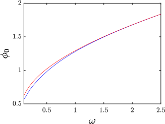
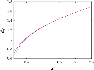
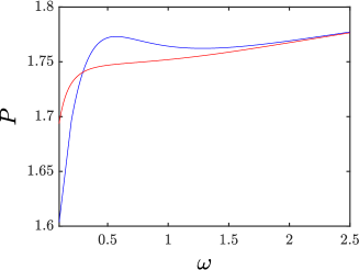
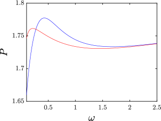
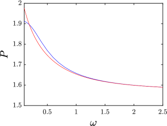
Figure 6: The amplitude ($\phi_{0}$) and norm-like quantity $P$ of 1-site discrete solitons (top and bottom panels, respectively) versus $\omega$ for $\sigma=1.7$ (left panels), $\sigma=1.75$ (middle panels) and $\sigma=2$ (right panels), fixing $C=1$. Blue (red) line corresponds to the numerical (variational) solution.

Finally, we mention the main features of unstable discrete solitons evolution for different typical examples of the instability that are identified above. Figures 7 and 8 show the outcome of the evolution for unstable 1-site solitons with $\sigma>1$: it is observed that the soliton density at $n=0$, $|\psi_{0}|^{2}$, deviates from the equilibrium value and subsequently performs oscillations around a new equilibrium value. In cases when bistability takes place, as, e.g., at $\sigma=1.7$ in Fig. 7, the unstable dynamical evolution, depending on a particular choice of the initial perturbation, may result in oscillations around states belonging, in the top and bottom panels, to two different branches of stable solutions. One can also observe that the soliton sustains together with the increasing of the density at $n=0$, a narrowing during the oscillations that manifest e.g. as a simultaneous decreasing of $|\psi_{\pm 1}|^{2}$. In addition, the maximum of $|\psi_{0}|^{2}$ increases with $\sigma$, and for $\sigma=1.8634$ it leads to computational overflow. Beyond this limit, despite using multiple algorithms, we have been unable to converge to a solution. Because of this, we cannot go beyond this value of $\sigma$ in our simulations. Our phenomenology basically involves an extremely fast increasing of $|\psi_{0}|^{2}$ that cannot be compensated by the decreasing of the term $(\psi_{1}+\psi_{-1})$ and hence, our numerical integrators fail to converge. It is important to note here that contrary to the DNLS case or the cubic nonlinearity limit (i.e. of logarithmic divergence), the conservation laws in the present case do not a priori preclude the density of a single site from becoming infinite. Clearly, identifying the phenomenology of the model for sufficiently large $\sigma$ is an important open topic that merits considerable additional study including from a theoretical point of view.

The dynamics of unstable 2-site solitons with $\sigma>1$ is somewhat different when $\sigma$ is close to 1. If $\sigma$ is close enough to 1 (as e.g. $\sigma=1.01$ for $\omega=C=1$), the soliton becomes mobile but, if $\sigma-1$ is high enough (as e.g. $\sigma=1.05$ for $\omega=C=1$), the soliton gets pinned and its profile oscillates between a 1-site and 2-site soliton (see Fig. 9). When $\sigma$ is increased (as e.g. to $\sigma=1.2$ for $\omega=C=1$), one can observe that the soliton undergoes a breaking of the symmetry between its two central sites (here, these are $n=-1$ and $n=0$). As a result, a dominant fraction of the mass concentrates at one of the two sites, e.g., at $n=0$, although a relatively high density remains at $n=-1$ too, decreasing with the increase of $\sigma$ (see Fig. 10). The high density fraction that concentrates at $n=0$ experiences a similar trend to the observed in the 1-site case.

It is also worthy to mention that unstable 1-site solitons with $\sigma<1$ feature mobility in the underlying lattice (not shown here in detail), which is a consequence of the stability-exchange bifurcation associated with the translational perturbation mode.

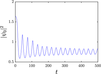
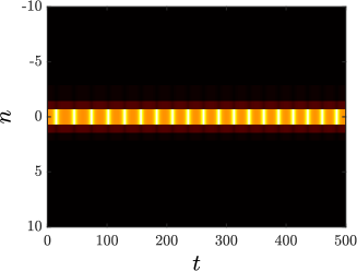
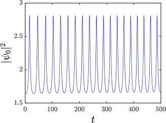
Figure 7: The evolution of the soliton density (left panel) and central-site density (right panel) for 1-site solitons with $\omega=C=1$ and $\sigma=1.7$. In the top (bottom) row, the soliton is perturbed along direction $\{a_{n}\}$ ($\{b_{n}\}$), with $[\{a_{n}\},\{b_{n}\}]$ being the eigenvector corresponding to the most unstable eigenvalue.

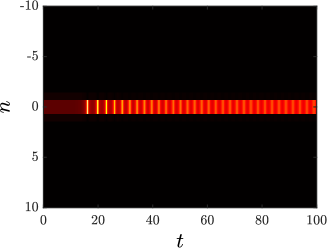
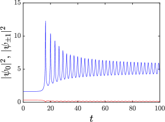
Figure 8: The evolution of the soliton density (left panel) and the central sites density (right panel) for the 1-site soliton with $\omega=C=1$ and $\sigma=1.8$. A small random perturbation was added to the (unstable) discrete solitons.

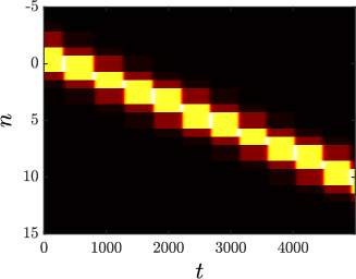
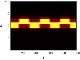
Figure 9: The evolution of the soliton density for 2-site solitons with $\omega=C=1$ and $\sigma=1.01$ (left panel), and $\sigma=1.05$ (right panel). In this case too, a small random perturbation was added to the unstable discrete solitons.

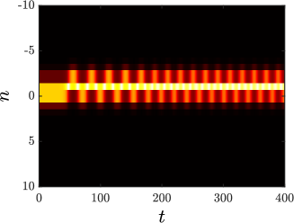
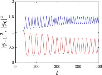
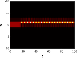
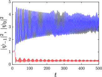
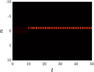
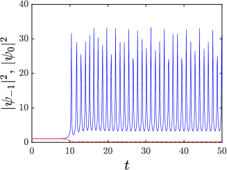
Figure 10: The evolution of the soliton density (left panel) and the central sites density (right panel) for 2-site solitons with $\omega=C=1$ and $\sigma=1.2$, $\sigma=1.5$, or $\sigma=1.7$ (top, middle, and bottom rows, respectively). In this case too, a small random perturbation was added to the unstable discrete solitons.

IV Conclusions and future challenges

In the present work we have explored a non-integrable generalization of the AL (Ablowitz-Ladik) model, bearing the power-law nonlinearity. The model by itself is interesting for a variety of reasons, such as the discretization of the continuum problem with the power-law nonlinearity, an extension of the integrable AL model, the mean-field limit of the Bose-Hubbard lattice with the population-dependent inter-site coupling, and as a testbed for addressing the interplay of discreteness and the potential for collapse (for a sufficiently large nonlinearity power, $\sigma$).

Our analysis has revealed essential features of the model. We have identified its conservation laws, including an unprecedented form of the conserved quantity (which falls back to the well-known logarithmic expression for the AL norm at $\sigma=1$) and the Hamiltonian. We have demonstrated how the modified norm-like quantity can be used (through its frequency dependence) to predict potential changes of stability, by means of the extended VK (Vakhitov-Kolokolov) criterion. We have also formulated the VA (variational approximation) based on the exponential ansatz, which is well capable of capturing the amplitude of the discrete solitons, but is considerably less accurate (due to limitations imposed by the fixed form of the analytically tractable ansatz) in capturing the quantity $P$, and, hence, the corresponding VK-predicted stability changes. We have identified a number of stability alternations between the 1- and 2-site (alias site- and inter-site-centered) modes, and addressed their dynamical implications. Importantly, for sufficiently large $\sigma$, the present model, on the contrary to the standard DNLS equation, appears to feature extreme amplitudes, which are not precluded a priori from the conservation laws. Whether indeed some form of collapse is present is an intriguing question that merits further study both from a theoretical and from a numerical perspective.

The present study paves the way for numerous questions worthwhile of further examination. Elaborating a better variational ansatz, if it may be (semi-) analytically tractable, will certainly help to develop more accurate understanding of the model’s features. An exploration of stability switchings, such as the one at the above-mentioned stability-exchange point $\sigma_{t}$, and of the origin of these phenomena, are certainly relevant issues in their own right. Extending the model to higher dimensions, and, in particular, the study of phenomenology of discrete vortices book is relevant too, while higher-dimensional AL models were, thus far, addressed in a very limited set of studies lafortune ; xiaowu . Lastly, as regards the focusing case with $\beta=1$, it should be interesting to address a possibility of the existence of rogue-wave modes, such as the (discrete variant of the) Peregrine soliton akhm ; yang . At the same time, exploring the defocusing case with $\beta=-1$ and the corresponding discrete dark solitons, as well as delocalized vortices, would be a subject of interest in its own right. Efforts along some of these directions are currently in progress and will be reported in future studies.

Acknowledgements. J.C.-M. thanks the financial support from MAT2016-79866-R project (AEI/FEDER, UE). P.G.K. acknowledges the support by NPRP grant # [9-329-1-067] from Qatar National Research Fund (a member of Qatar Foundation). The work of B.A.M. was supported, in part, by the Israel Science Foundation, through grant No. 1287/17. This material is also based upon work supported by the National Science Foundation under Grant No. PHY-1602994 (P.G.K.).

Findings reported herein are solely the responsibility of the authors.

References

- (1) P. G. Kevrekidis, The Discrete Nonlinear Schrödinger Equation, Springer-Verlag (Heidelberg, 2009).
- (2) C. Sulem and P. L. Sulem, The Nonlinear Schrödinger Equation (Springer-Verlag, New York, 1999).
- (3) M. J. Ablowitz, B. Prinari, and A. D. Trubatch, Discrete and Continuous Nonlinear Schrödinger Systems, Cambridge University Press (Cambridge, 2004).
- (4) P. G. Kevrekidis, D. J. Frantzeskakis, and R. Carretero-González, The defocusing Nonlinear Schrödinger Equation: From Dark Solitons to Vortices and Vortex Rings (SIAM, Philadelphia, 2015).
- (5) D. N. Christodoulides, F. Lederer, and Y. Silberberg, Nature 424, 817 (2003); A. A. Sukhorukov, Y. S. Kivshar, H. S. Eisenberg, and Y. Silberberg, IEEE J. Quant. Elect. 39, 31 (2003).
- (6) F. Lederer, G. I. Stegeman, D. N. Christodoulides, G. Assanto, M. Segev, and Y. Silberberg, Phys. Rep. 463, 1 (2008).
- (7) O. Morsch and M. Oberthaler, Rev. Mod. Phys. 78, 179 (2006).
- (8) M. Peyrard, Nonlinearity 17, R1 (2004).
- (9) C. Chong, P. G. Kevrekidis, Coherent Structures in Granular Crystals: From Experiment and Modelling to Computation and Mathematical Analysis, Springer Verlag (Heidelberg, 2018).
- (10) A. K. Sieradzan, A. Niemi, and X. Peng, Phys. Rev. E 90, 062717 (2004).
- (11) M. J. Ablowitz, J. F. Ladik, J. Math. Phys. 16, 598 (1975); ibid. 17, 1011 (1976).
- (12) T. Kapitula, P. Kevrekidis, Nonlinearity 14, 533 (2001).
- (13) D. Cai, A. R. Bishop, N. Grønbech-Jensen, and M. Salerno Phys. Rev. Lett. 74, 1186 (1995).
- (14) M. Salerno, Phys. Rev. A 46, 6856 (1992).
- (15) D. Cai, A. R. Bishop, and N. Grønbech-Jensen Phys. Rev. E 53, 4131 (1996).
- (16) O. Dutta, M. Gajda, P. Hauke, M. Lewenstein, D.-S. Luhmann, B. Malomed, T. Sowinski, and J. Zakrzewski, Rep. Prog. Phys. 78, 066001 (2015).
- (17) S. V. Dmitriev, P. G. Kevrekidis, B. A. Malomed, and D. J. Frantzeskakis Phys. Rev. E 68, 056603 (2003).
- (18) A. Ankiewicz, N. Akhmediev, and J. M. Soto-Crespo Phys. Rev. E 82, 026602 (2010).
- (19) Y. Ohta and J. Yang, J. Phys. A: Math. Theor. 47, 255201 (2014).
- (20) C. Hoffmann, E. G. Charalampidis, D. J. Frantzeskakis, P. G. Kevrekidis, arXiv:1710.04899.
- (21) E. W. Laedke, K. H. Spatschek, and S. K. Turitsyn, Phys. Rev. Lett. 73, 1055 (1994).
- (22) B.A. Malomed, M. I. Weinstein, Phys. Lett. A 220, 91 (1996).
- (23) M. I. Weinstein, Nonlinearity 12, 673 (1999).
- (24) J. Cuevas, P. G. Kevrekidis, D. J. Frantzeskakis, B.A. Malomed, Physica D 238, 67 (2009).
- (25) S. Flach, K. Kladko, R. S. MacKay, Phys. Rev. Lett. 78, 1207 (1997).
- (26) D. S. Petrov and G. E. Astrakharchik, Phys. Rev. Lett. 117, 100401 (2016).
- (27) G. E. Astrakharchik and B. A. Malomed, Phys. Rev. A 98, 013631 (2018).
- (28) M. Vakhitov and A. Kolokolov, Radiophys. Quantum Electron. 16, 783 (1973).
- (29) B.A. Malomed, Progr. Opt. 43, 69 (2002).
- (30) M. Grillakis, J. Shatah, W. Strauss, J. Funct. Anal. 74, 160 (1987); J. Funct. Anal. 94, 308 (1990).
- (31) C. Chong, D. E. Pelinovsky, G. Schneider, Physica D 241, 115 (2012).
- (32) T. Kapitula, K. Promislow, Spectral and dynamical stability of nonlinear waves, Springer-Verlag (New York, 2013).
- (33) P. G. Kevrekidis, G. J. Herring, S. Lafortune, Q. E. Hoq, Phys. Lett. A 376, 982 (2012).
- (34) X. Y. Wu, B. Tian, L. Liu, Y. Sun, Comm. Nonlin. Sci. Num. Simul. 50, 201 (2017).