Abstract

This paper is concerned with the inverse problem to recover a compactly supported Schrödinger potential given the differential scattering cross section, i.e. the modulus, but not the phase of the scattering amplitude. To compensate for the missing phase information we assume additional measurements of the differential cross section in the presence of known background objects. We propose an iterative scheme for the numerical solution of this problem and prove that it converges globally of arbitrarily high order depending on the smoothness of the unknown potential as the energy tends to infinity. At fixed energy, however, the proposed iteration does not converge to the true solution even for exact data. Nevertheless, numerical experiments show that it yields remarkably accurate approximations with small computational effort even for moderate energies. At small noise levels it may be worth to improve these approximations by a few steps of a locally convergent iterative regularization method, and we demonstrate to which extent this reduces the reconstruction error.

Keywords: Inverse scattering problems, phaseless inverse scattering, Schrödinger equation

AMS subject classification: 35J10, 35R30, 65N21, 81U40, 78A46

1 Introduction

In quantum mechanics the interaction of an elementary particle at fixed energy $E>0$ with a macroscopic object contained in a bounded domain $D$ is described by the Schrödinger equation

$$-\Delta\psi+v(x)\psi=E\psi,\quad x\in\mathbb{R}^{d}.$$ (1.1a)

Here $$\Delta x v$$ is the standard Laplacian in , and the potential function is assumed to satisfy

$$v\in L^{\infty}(\mathbb{R}^{d}),\quad\operatorname{supp}v\subset D\subset\mathbb{R}^{d},d\geq 2.$$ (1.1b)

Equation (1.1a) can be also considered as the Helmholtz equation of acoustic and electrodynamic wave propagation at fixed frequency.

For equation (1.1a) we consider the classical scattering solutions $\psi^{+}(\cdot,k)$ of the form $\psi^{+}(x,k)=e^{ikx}+\psi^{\rm s}(x,k)$ with a plane incident field $e^{ikx}$ such that $k\in\mathbb{R}^{d}$, $|k|^{2}=E$, and a scattered field $\psi^{\rm s}(\cdot,k)$ satisfying the Sommerfeld radiation condition

$$|x|^{\frac{d-1}{2}}\left(\frac{\partial}{\partial|x|}-i|k|\right)\psi^{\rm s}(x,k)\to 0\qquad\mbox{as }|x|\to\infty$$ (1.1c)

uniformly in $x/|x|$. This implies that $\psi^{\rm s}$ has the asymptotic behavior

$$\psi^{\rm s}(x,k)=c(d,|k|)\frac{e^{i|k||x|}}{|x|^{\frac{d-1}{2}}}f_{E}\left(k,|k|\tfrac{x}{|x|}\right)+\mathcal{O}\left(|x|^{-\frac{d+1}{2}}\right),\quad|x|\to\infty,$$ (1.2)

$$c(d,|k|):=-\pi i(-2\pi i)^{(d-1)/2}|k|^{(d-3)/2}$$

with a function $f_{E}$ called the scattering amplitude or far field pattern at energy $E$. There are different conventions for the choice of the constant $c(d,|k|)$. The one above leads to the following simple asymptotic relation between the scattering amplitude and the inverse Fourier transform of $v$, see, e.g., [Fad1956, Nov2015en]:

$$\widehat{v}(k-l)=f_{E}(k,l)+\mathcal{O}(E^{-\frac{1}{2}}),\quad E\to+\infty,$$ (1.3)

$$\widehat{v}(p):=(2\pi)^{-d}\int_{\mathbb{R}^{d}}e^{ipx}v(x)\,dx,\quad p\in\mathbb{R}^{d}$$ (1.4)

$|f_{E}(k,l)|^{2}$ is known as the differential scattering cross section for equation (1.1a). In quantum mechanics this quantity describes the probability density of scattering of particle with initial impulse $k$ into direction $l/|l|\neq k/|k|$, see, for example, [Fad1993, Chapter 1, Section 6]. Typically, the differential cross section is the only measurable quantity whereas the phase of the scattering amplitude cannot be determined directly by physical experiments. The problem of finding $v$ from $|f_{E}|^{2}$ is known as the phaseless inverse scattering problem for equation (1.1a). Whereas the inverse scattering problem with phase information for equation (1.1a), i.e. the problem of finding $v$ from $f_{E}$, has been studied intensively for a long time (see [Alex2008, Barc2016, Bur2009en, Chad1989, Eskin2011, Fad1956, Grin2000, Haeh2001, Isay2013b, Isay2013c, Nov1988en, Nov1998, Nov2005b, Nov2013b, Nov2015en] and references therein), much less studies were performed in the phaseless case (see [Agal2016b, Chad1989, Klib2014, Klib2016a, romanov2018phaseless, Nov2015LS, Nov2015b, Nov2016]).

It is well known that the phaseless scattering data $|f_{E}|^{2}$ does not determine $v$ uniquely even if $|f_{E}|^{2}$ is given completely for all $E>0$; see, e.g., [Nov2016]. In the present work we continue studies of [Nov2016, Agal2016b] assuming additional measurements of the following form: For the unknown $v$ satisfying (1.1b) we consider additional a priori known background scatterers $w_{1}$, …, $w_{L}$ such that

$$\begin{gathered}w_{l}\in L^{\infty}(\mathbb{R}^{d}),\quad\operatorname{supp}w_{l}\subset\Omega_{l},\\ \text{$\Omega_{l}$ is an open bounded domain in $\mathbb{R}^{d}$},\\ w_{l}\neq 0,\quad\text{$w_{l}\neq w_{\tilde{l}}$ if $l\neq\tilde{l}$ (in $L^{\infty}(\mathbb{R}^{d}$)),}\end{gathered}$$ (1.5)

where $l,\tilde{l}\in\{1,\ldots,L\}$. In practice, we also typically have

$$\Omega_{l}\cap D=\varnothing,$$

but this property will not be needed in our analysis. We set

$$S=\{|f_{E}|^{2},|f_{E,1}|^{2},\ldots,|f_{E,L}|^{2}\},$$ (1.6)

where $f_{E}$ is the scattering amplitude for $v$ at energy $E$, and $f_{E,1}$, …, $f_{E,L}$ are the scattering amplitudes for $v_{1}$, …, $v_{L}$, where

$$v_{l}=v+w_{l},\quad l=1,\ldots,L.$$ (1.7)

One can see that $S$ consists of the phaseless scattering data $|f_{E}|^{2}$, $|f_{E,1}|^{2}$, …, $|f_{E,L}|^{2}$ measured sequentially, first, for the unknown scatterer $v$ and then for the unknown scatterer $v$ in the presence of known scatterer $w_{l}$ disjoint from $v$ for $l=1$, …, $L$. We consider the following inverse scattering problem without phase information for equation (1.1a):

Problem 1.

Reconstruct coefficient $v$ from the phaseless scattering data $S$ for some appropriate background scatterers $w_{1}$, …, $w_{L}$.

In this paper we propose an iterative approach to Problem 1 with iterates $u^{(j)}_{E}$, $j=1,2,\dots$ and prove error bounds of the form

$$\|u^{(j)}_{E}-v\|_{L^{\infty}}=\mathcal{O}\left(E^{-\alpha_{j}}\right)$$ (1.8)

with exponents $\alpha_{j}$ tending to $\infty$ as $j\to\infty$ for infinitely smooth potentials $v$.

For the inverse scattering problem with phase information such a substantial improvement of the Born approximation, which serve as first iterate $u_{1}$ (see (1.3)) has been obtained in [Nov2015en], and first numerical tests were reported in [Barc2016].

Studies on Problem 1 in dimension $d=1$ for $L=1$ were started in [Akto1998], where phaseless scattering data was considered for all $E>0$. Note also that a phaseless optical imaging in the presence of known background objects was considered, in particular, in [Gov2009]. Studies on Problem 1 in dimension $d\geq 2$ were started in [Nov2016] and continued recently in [Agal2016b]. The key result of [Nov2016] consists in a proper extension of formula (1.3) for the Fourier transform $\widehat{v}$ of $v$ to the phaseless case of Problem 1, $d\geq 2$, which will be detailed in Section 3.1. The main results of [Agal2016b] consist in proper extensions of formula (2.8) in the configuration space to the case of Problem 1 for $d\geq 2$; see also Section 3.1. However, the convergence of the approximations to $v$ as $E\to+\infty$ in [Agal2016b] is slow, in particular, the exponent $\alpha$ in (1.8) is always $\leq\frac{1}{2}$.

In addition, our theoretical iterative monochromatic reconstructions for Problem 1 are illustrated numerically in Section 4.

2 Iterative inversion with phase information

2.1 Inverse scattering with phase information

Recall that the scattering amplitude $f_{E}$ is defined on the set

$$\mathcal{M}_{E}=\bigl{\{}(k,l)\in\mathbb{R}^{d}\times\mathbb{R}^{d}\colon|k|^{2}=|l|^{2}=E\bigr{\}}.$$ (2.1)

In view of (1.3) we assume that the scattering amplitude, and later the differential cross section is defined on some subset $\mathcal{M}^{\mathrm{m}}_{E}\subset\mathcal{M}_{E}$ such that the function

$$\tilde{\Phi}\colon\mathcal{M}^{\mathrm{m}}_{E}\to\mathcal{B}^{d}_{2\sqrt{E}}\qquad\tilde{\Phi}(k,l):=k-l$$ (2.2)

is surjective. Here and in the following $\mathcal{B}^{d}_{r}$ denotes the closed ball

$$\mathcal{B}^{d}_{r}=\bigl{\{}p\in\mathbb{R}^{d}\colon|p|\leq r\bigr{\}},\quad r>0.$$ (2.3)

For $d\geq 2$ we may construct a $d$-dimensional subset $\mathcal{M}^{\mathrm{m}}_{E}\subset\mathcal{M}_{E}$ such that $\tilde{\Phi}$ is bijective as follows: Let us choose a piece-wise continuous function $\gamma:\mathbb{\mathcal{missing}}B^{d}_{2\sqrt{E}}\to\mathbb{R}^{d}$ such that $|\gamma(p)|=1$ and $\gamma(p)p=0$ for all $p\in\mathcal{B}^{d}_{2\sqrt{E}}$ and set

$$\mathcal{M}^{\mathrm{m}}_{E}=\left\{\left(\tfrac{p}{2}+\bigl{(}E-\tfrac{p^{2}}{4}\bigr{)}^{1/2}\gamma(p),-\tfrac{p}{2}+\bigl{(}E-\tfrac{p^{2}}{4}\bigr{)}^{1/2}\gamma(p)\right)\colon p\in\mathcal{B}^{d}_{2\sqrt{E}}\right\}.$$ (2.4)

To use the Born approximation (1.3) and its refinements if $\tilde{\Phi}$ is not injective, we average over the set $\tilde{\Phi}^{-1}(p)$. To this end we assume that for all $p\in\mathcal{B}^{d}_{2\sqrt{E}}$ the set $\tilde{\Phi}^{-1}(p)$ is a piecewise smooth manifold of size $\left|\tilde{\Phi}^{-1}(p)\right|$ and define the averaging operator

$$\Phi:L^{1}(\mathcal{M}^{\mathrm{m}}_{E})\to L^{1}\left(\mathcal{B}^{d}_{2\sqrt{E}}\right),\qquad(\Phi f)(p):=\tfrac{1}{\left|\tilde{\Phi}^{-1}(p)\right|}\int_{\tilde{\Phi}^{-1}(p)}f_{E}(k,l)\,d(k,l).$$ (2.5)

Using this mapping we can define an approximation $u_{E}$ to $v$ on $D$ by

$$u_{E}(x):=\int_{\mathcal{B}^{d}_{2\sqrt{E}}}e^{-ipx}(\Phi f)(p)\,dp,\qquad x\in D.$$ (2.6)

Let $W^{n,1}(\mathbb{R}^{d})$ denote the Sobolev space of $n$-times smooth functions in the sense of $L^{1}(\mathbb{R}^{d})$:

$$W^{n,1}(\mathbb{R}^{d}):=\bigl{\{}u\in L^{1}(\mathbb{R}^{d})\colon\|u\|_{n,1}<\infty\bigr{\}}\quad\mbox{with}$$ (2.7)

$$\|u\|_{n,1}:=\max\limits_{|J|\leq n}\left\|\frac{\partial^{|J|}u}{\partial x^{J}}\right\|_{L^{1}(\mathbb{R}^{d})},\quad n\in\mathbb{N}\cup\{0\}.$$

If $v\in W^{n,1}(\mathbb{R}^{d})$, $n>d$, in addition to the initial assumptions (1.1b), then $u_{E}$ satisfies the error bound

$$\|u_{E}-v\|_{L^{\infty}(D)}=\mathcal{O}(E^{-\alpha})\quad\mbox{as $E\to+\infty$}\qquad\mbox{with }\alpha=\frac{n-d}{2n}$$ (2.8)

for $d\geq 2$; see, for example, [Nov2015en]. Essential improvements of the approximation $u_{E}$ in (2.6) were achieved in [Nov1998, Nov2005b, Nov2015en]. In particular, formula (2.8) was principally improved in [Nov2015en] by constructing iteratively nonlinear approximate reconstructions $u^{(j)}_{E}$ such that $u^{(1)}_{E}=u_{E}$ and

$$\begin{gathered}\|u^{(j)}_{E}-v\|_{L^{\infty}(D)}=\mathcal{O}(E^{-\alpha_{j}})\quad\text{with }\alpha_{j}=\tfrac{n-d}{2d}\left(1-\left(\tfrac{n-d}{n}\right)^{j}\right),\quad j\geq 1,\end{gathered}$$ (2.9)

as $E\to+\infty$ for $d\geq 2$ if $v\in W^{n,1}(\mathbb{R}^{d})$, $n>d$, in addition to the initial assumptions (1.1b). The point is that

$$\alpha_{j}\to\alpha_{\infty}=\tfrac{n-d}{2d} \text{as $j\to+\infty$},$$ (2.10)

$$\alpha_{j}\to\tfrac{j}{2} \text{as $n\to+\infty$},$$

$$\alpha_{\infty}\to+\infty \text{as $n\to+\infty$};$$

that is the convergence in (2.9) as $E\to+\infty$ is drastically better than the convergence in (2.8), at least, for large $n$ and $j$.

2.2 Iterative step for phased inverse scattering

Recall that the outgoing fundamental solution to the Helmholtz equation is given by

$$G^{+}(x,k)=-(2\pi)^{-d}\int_{\mathbb{R}^{d}}\frac{e^{i\xi x}d\xi}{\xi^{2}-k^{2}-i0}=\frac{i}{4}\big{(}\frac{k}{2\pi|x-y|}\big{)}^{\nu}H^{(1)}_{\nu}(k|x-y|)\quad\mbox{with}\quad\nu:=\tfrac{d}{2}-1,$$

where $H^{(1)}_{\nu}$ denotes the Hankel function of the first kind of order $\nu$. Let $\mathcal{G}^{+}(k)$ denote the convolution operator with kernel $G^{+}(\cdot,k)$. The following estimate, which goes back to [Agmon1975], is essential for studies on direct scattering (see, e.g., [Eskin2011] (§29), [Nov2015en], and references therein) and will also be crucial for our analysis:

$$\begin{gathered}\|\Lambda^{-s}\mathcal{G}^{+}(k)\Lambda^{-s}\|_{L^{2}(\mathbb{R}^{d})\to L^{2}(\mathbb{R}^{d})}\leq a_{0}(d,s)|k|^{-1},\\ k\in\mathbb{R}^{d},\;|k|\geq 1,\quad\text{for $s>\tfrac{1}{2}$}.\end{gathered}$$ (2.11)

Here $\Lambda^{-s}$ denotes the operator of multiplication by $(1+|x|^{2})^{-s/2}$.

Let $v$, satisfying (1.1b), be the unknown potential and $v^{*}_{E}$ be an approximation to $v$, and assume that there exist constants $A,E^{*},K,\alpha>0$ such that

$$v^{*}_{E}\in L^{\infty}(\mathbb{R}^{d}),\quad\operatorname{supp}v^{*}_{E}\subset D$$ (2.12a)

$$\|v^{*}_{E}-v\|_{L^{\infty}(D)}\leq AE^{-\alpha}$$ (2.12b)

$$\|v\|_{L^{\infty}(\mathbb{R}^{d})}\leq K,\quad\|v^{*}_{E}\|_{L^{\infty}(\mathbb{R}^{d})}\leq K$$ (2.12c)

for all $E\geq E^{*}$.

For inverse scattering with phase information the iterative step of [Nov2015en] is based on the following lemma.

Lemma 2.1.

Let $v$, satisfying (1.1b), be the unknown potential and $v^{*}(\cdot,E)$ be an approximation to $v$ satisfying (2.12) for some $A>0$, $\alpha\geq 0$, $K>0$ and $E^{*}=E^{*}(K,D)$, where

$$\begin{gathered}E^{*}(K,D)=2Ka_{0}(d,s)\sup_{x\in D}(1+|x|^{2})^{s/2},\\ \text{for some $s>\tfrac{1}{2}$, where $a_{0}(d,s)$ is the constant of \eqref{in.Agmon}}.\end{gathered}$$ (2.13)

Let $f_{E}$, $f^{*}_{E}$ be the scattering amplitudes of $v$, $v^{*}_{E}$. Then there exists a constant $\mu_{1,\S\ref{sec.itp}}=\mu_{1,\S\ref{sec.itp}}(A,K,D)>0$ such that

$$\sup_{(k,l)\in\mathcal{M}_{E}}|f_{E}(k,l)-f^{*}_{E}(k,l)+\widehat{v^{*}_{E}}(k-l)-\widehat{v}(k-l)|\leq\mu_{1,\S\ref{sec.itp}}E^{-\alpha-\frac{1}{2}},\quad E\geq E^{*},$$ (2.14)

where $\widehat{v}$, $\widehat{v^{*}_{E}}$ are the Fourier transforms of $v$, $v^{*}_{E}$ defined according to (1.4).

Note that in this paper we use the notation $\mu_{k,\S X}$, $k\geq 1$, for the constants of Section X.

Lemma 2.1 follows from Lemma 3.2 of [Nov2015en] for $v_{0}\equiv 0$, where $v_{0}$ is the background potential of [Nov2015en]. The proof of Lemma 3.2 of [Nov2015en] essentially uses estimate (2.11).

In particular, due to (2.14), the function

$$U^{**}_{E}:=\Phi f_{E}-\Phi f^{*}_{E}+\widehat{v^{*}_{E}},$$ (2.15)

where $\Phi f_{E}$, $\Phi f^{*}_{E}$ are defined according to (2.5), satisfies the following improved error estimate compared to (2.12b):

$$\|U^{**}_{E}-\widehat{v}\|_{L^{\infty}(\mathcal{B}^{d}_{2\sqrt{E}})}\leq\mu_{1,\S\ref{sec.itp}}E^{-\alpha-\frac{1}{2}},\qquad E\geq E^{*}.$$ (2.16)

If $v\in W^{n,1}(\mathbb{R}^{d})$, $n>d$ (in addition to the initial assumptions (1.1b)), and if

$$\alpha<\tfrac{n}{2d}-\tfrac{1}{2},$$ (2.17)

then this permits to construct an improved approximation $v^{**}_{E}$ to the unknown potential $v$ as follows:

$$\begin{gathered}v^{**}_{E}(x):=\begin{cases}\int_{\mathcal{B}^{d}_{r(E)}}e^{-ipx}U^{**}_{E}(p)\,dp,&x\in D,\\ 0,&x\not\in D,\end{cases}\qquad r(E):=2\tau E^{\frac{1+2\alpha}{2n}},\quad\tau\in(0,1],\end{gathered}$$ (2.19)

Here $U^{**}_{E}$ is defined in (2.15) and $E^{*}=E^{*}(K,D)$ is the constant of (2.13). It follows that there exists a constant $B>0$ such that

$$\|v^{**}_{E}-v\|_{L^{\infty}(D)}\leq BE^{-\beta},\quad E\geq E^{*}\mbox{ with }\beta:=\alpha(1-\tfrac{d}{n})+\tfrac{1}{2}-\tfrac{d}{2n},$$ (2.20)

Note that

$$\alpha<\beta<\tfrac{n}{2d}-\tfrac{1}{2}$$

and that condition (2.17) implies that $r(E)\leq 2\sqrt{E}$, so that the definition (2.19) is correct.

3 Iterative inversion from phaseless data

3.1 Low order potential reconstruction formulas from phaseless data

In this subsection we extend the formulas (1.3) and (2.8) to the phaseless case. The key result of [Nov2016] consists in the following formulas for solving Problem 1 in dimension $d\geq 2$ for $L=2$ at high energies $E$:

$$\begin{gathered}\sup_{p\in\mathcal{B}^{d}_{2\sqrt{E}}}\left||\widehat{v_{l}}(p)|^{2}-|\Phi f_{E,l}(p)|^{2}\right|=\mathcal{O}(E^{-\frac{1}{2}}),\quad E\to+\infty,\quad l=0,1,2,\end{gathered}$$ (3.1)

where $v_{0}=v$, $v_{l}$ is defined by (1.7), $l=1$, $2$, $f_{E,0}=f_{E}$, $f_{E,1}$, $f_{E,2}$ are the scattering amplitudes for $v_{0}$, $v_{1}$, $v_{2}$, respectively; in addition,

$$\begin{pmatrix}\mathop{\mathrm{Re}}\widehat{v}\\ \mathop{\mathrm{Im}}\widehat{v}\end{pmatrix}=\frac{1}{2}\begin{pmatrix}\mathop{\mathrm{Re}}\widehat{w_{1}}&\mathop{\mathrm{Im}}\widehat{w_{1}}\\ \mathop{\mathrm{Re}}\widehat{w_{2}}&\mathop{\mathrm{Im}}\widehat{w_{2}}\end{pmatrix}^{-1}\begin{pmatrix}|\widehat{v_{1}}|^{2}-|\widehat{v}|^{2}-|\widehat{w_{1}}|^{2}\\ |\widehat{v_{2}}|^{2}-|\widehat{v}|^{2}-|\widehat{w_{2}}|^{2}\end{pmatrix},$$ (3.2)

where $\widehat{v}=\widehat{v}(p)$, $\widehat{v_{l}}=\widehat{v}_{l}(p)$, $\widehat{w_{l}}=\widehat{w}_{l}(p)$, $p\in\mathbb{R}^{d}$, and formula (3.2) is considered for all $p$ such that the determinant

$$\zeta_{\widehat{w_{1}},\widehat{w_{2}}}(p):=\mathop{\mathrm{Re}}\widehat{w_{1}}(p)\mathop{\mathrm{Im}}\widehat{w_{2}}(p)-\mathop{\mathrm{Im}}\widehat{w_{1}}(p)\mathop{\mathrm{Re}}\widehat{w_{2}}(p)\neq 0.$$ (3.3)

Formulas (3.1), (3.2) can be considered as a natural extension of formula (1.3) to the phaseless case of Problem 1, $d\geq 2$, $L=2$ and lead to the function $\mathrm{Urec}$ defined in Algorithm 1 for the approximate reconstruction $U_{\widehat{w_{1}},\widehat{w_{2}}}$ of $\widehat{v}$:

$$U_{\widehat{w_{1}},\widehat{w_{2}}}(p):=\mathrm{Urec}\left(\widehat{w_{1}}(p),\widehat{w_{2}}(p),\Phi|f_{E}|^{2}(p),\Phi|f_{E,1}|^{2}(p),\Phi|f_{E,2}|^{2}(p)\right),\qquad|p|\leq 2\sqrt{E}$$ (3.4)

Algorithm 1 $\mathrm{function}\;U=\texttt{Urec}(W_{1},W_{2},F,F_{1},F_{2})$

data: Fourier transforms of reference potentials at some point $p$: $W_{1}=\widehat{w}_{1}(p)$, $W_{2}=\widehat{w}_{2}(p)$;
scattering amplitude at $(k,l)$, $k-l=p$ without reference potential: $F=|f(k,l)|^{2}$
scattering amplitudes with reference potentials: $F_{1}=|f_{1}(k,l)|^{2}$, $F_{2}=|f_{2}(k,l)|^{2}$
result: approximation to the Fourier transform of the unknown potential $v$ at $p$: $U\approx\widehat{v}(p)$

$M:=\left(\begin{array}[]{cc}\mathop{\mathrm{Re}}W_{1}&\mathop{\mathrm{Im}}W_{1}\\ \mathop{\mathrm{Re}}W_{2}&\mathop{\mathrm{Im}}W_{2}\end{array}\right)$; $b:=\left(\begin{array}[]{c}F_{1}-F-|W_{1}|^{2}\\ F_{2}-F-|W_{2}|^{2}\end{array}\right)$; $\left(\begin{array}[]{c}x\\ y\end{array}\right):=\frac{1}{2}M^{-1}b$; $U:=x+iy$

On the level of analysis (e.g., error estimates), the principal complication of (3.1), (3.2) in comparison with (1.3) consists in possible zeros of the determinant $\zeta_{\widehat{w_{1}},\widehat{w_{2}}}$ of (3.3). This complication is, in particular, essential if one tries to transform (3.1), (3.2) into an approximate reconstruction in the configuration space, applying the inverse Fourier transform to $\widehat{v}=\mathop{\mathrm{Re}}\widehat{v}+i\mathop{\mathrm{Im}}\widehat{v}$ of (3.2). For some simplest cases, the results of transforming (3.1), (3.2) to approximate reconstructions in the configuration space, including error estimates, were given in [Agal2016b].

Background potentials of type A: The first simplest case analyzed in [Agal2016b] is

$$w_{1}(x):=w(x-T_{1}),\quad w_{2}(x):=iw(x-T_{1}),\quad x\in\mathbb{R}^{d},$$ (3.5)

$$\begin{aligned} &\mbox{for some }w\in C(\mathbb{R}^{d})\mbox{ such that }w=\overline{w},\;\text{$w(x)=0$ for $|x|>R$},\mbox{and}\\ &\widehat{w}(p)=\overline{\widehat{w}(p)}\geq\mu_{1,\S\ref{sec.pex}}(1+|p|)^{-\sigma},\quad p\in\mathbb{R}^{d},\end{aligned}$$ (3.6)

for some fixed $T_{1}\in\mathbb{R}^{d}$, $R>0$, $\mu_{1,\S\ref{sec.pex}}>0$, $\sigma>d$, where $T_{1}$ and $R$ are chosen in such a way that $w_{1}$ satisfies (1.5) (and, as a corollary, $w_{1}$, $w_{2}$ satisfy (1.5) with $\Omega_{2}=\Omega_{1}$). In addition, a broad class of $w$ satisfying (LABEL:pex.defw) was constructed in Lemma 1 of [Agal2016b]. One can see that

$$\begin{gathered}\zeta_{\widehat{w_{1}},\widehat{w_{2}}}(p)=|\widehat{w}(p)|^{2}\geq\mu_{1,\S\ref{sec.pex}}^{2}(1+|p|)^{-2\sigma},\quad p\in\mathbb{R}^{d},\\ \text{if $w_{1}$, $w_{2}$ are defined by \eqref{pex.defw1w2c}, \eqref{pex.defw}}.\end{gathered}$$ (3.7)

Background potentials of type B: The second simplest case analyzed in [Agal2016b] is

$$\begin{gathered}w_{1}(x)=w(x-T_{1}),\quad w_{2}(x)=w(x-T_{2}),\quad x\in\mathbb{R}^{d},\\ \text{for some fixed $T_{1},T_{2}\in\mathbb{R}^{d}$},\end{gathered}$$ (3.8)

where $w$ is the same as in (LABEL:pex.defw), and $T_{1}$, $T_{2}$, $R$ are chosen in such a way that $w_{1}$, $w_{2}$ satisfy (1.5). One can see that

$$\begin{gathered}\zeta_{\widehat{w_{1}},\widehat{w_{2}}}(p)=\sin(py)|\widehat{w}(p)|^{2},\quad y=T_{2}-T_{1}\neq 0,\quad p\in\mathbb{R}^{d},\\ |\zeta_{\widehat{w_{1}},\widehat{w_{2}}}(p)|\geq\mu_{1,\S\ref{sec.pex}}^{2}(1+|p|)^{-2\sigma}\tfrac{2\varepsilon}{\pi},\quad p\in\mathbb{R}^{d}\setminus Z^{\varepsilon}_{y},\\ \text{if $w_{1}$, $w_{2}$ are defined by \eqref{pex.defw}, \eqref{pex.defw1w2r},}\end{gathered}$$ (3.9)

where

$$Z^{\varepsilon}_{y}=\bigl{\{}p\in\mathbb{R}^{d}\colon py\in(-\varepsilon,\varepsilon)+\pi\mathbb{Z}\bigr{\}},\quad y\in\mathbb{R}^{d}\setminus 0,\;\;0<\varepsilon<1.$$ (3.10)

First consider background potentials $w_{1}$, $w_{2}$ of type A (see (3.5), (LABEL:pex.defw)) and assume that $v$ satisfies (1.1b), $v\in W^{n,1}(\mathbb{R}^{d})$ for some $n>d$. Then the result of transforming $U_{\widehat{w_{1}},\widehat{w_{2}}}$ in (3.4) by

$$\begin{gathered}u_{E}(x):=\int_{\mathcal{B}^{d}_{r(E)}}e^{-ipx}U_{\widehat{w_{1}},\widehat{w_{2}}}(p,E)\,dp,\quad x\in\mathbb{R}^{d},\\ r(E)=2\tau E^{\frac{\alpha}{n-d}}\quad\text{for some fixed $\tau\in(0,1]$},\end{gathered}$$ (3.11)

to an approximate reconstruction in the configuration space is as follows (see [Agal2016b, Theorem 1]):

$$\begin{gathered}\|u_{E}-v\|_{L^{\infty}(\mathbb{R}^{d})}=\mathcal{O}(E^{-\alpha})\quad\;E\to+\infty\quad\mbox{with }\alpha=\frac{\frac{1}{2}(n-d)}{n+\sigma}.\end{gathered}$$ (3.12)

Now consider background potentials $w_{1}$, $w_{2}$ of type B (see (3.8)) and assume again that $v$ satisfies (1.1b), $v\in W^{n,1}(\mathbb{R}^{d})$ for some $n>d$. We transform $U_{\widehat{w_{1}},\widehat{w_{2}}}$ in (3.4) to an approximation $u_{E}$ in the configuration space as follows:

$$\begin{gathered}u_{E}(x)=u_{E,1}(x)+u_{E,2}(x),\quad x\in\mathbb{R}^{d},\\ u_{E,1}(x)=\int\limits_{\mathcal{B}^{d}_{r(E)}\setminus Z^{\varepsilon(E)}_{y}}e^{-ipx}U_{\widehat{w_{1}},\widehat{w_{2}}}(p,E)\,dp,\\ u_{E,2}(x)=\int\limits_{\mathcal{B}^{d}_{r(E)}\cap Z^{\varepsilon(E)}_{y}}e^{-ipx}U^{\varepsilon(E)}_{\widehat{w_{1}},\widehat{w_{2}}}(p,E)\,dp,\\ r(E)=2\tau E^{\frac{\alpha}{n-d}},\quad\varepsilon(E)=E^{-\tfrac{\alpha}{2}}\quad\text{for some $\tau\in(0,1]$,}\end{gathered}$$ (3.13)

$Z^{\varepsilon}_{y}$ is defined in (3.10), and

$$U^{\varepsilon}_{\widehat{w_{1}},\widehat{w_{2}}}(p,E)=\tfrac{1}{2}\bigl{(}U_{\widehat{w_{1}},\widehat{w_{2}}}(p^{\varepsilon}_{-},E)+U_{\widehat{w_{1}},\widehat{w_{2}}}(p^{\varepsilon}_{+},E)\bigr{)},$$ (3.14)

$$\begin{gathered}p^{\varepsilon}_{\pm}=p_{\bot}+\pi z(p)\tfrac{y}{|y|^{2}}\pm\varepsilon\tfrac{y}{|y|^{2}},\quad p_{\bot}=p-(p\cdot y)\tfrac{y}{|y|^{2}},\quad p\in\mathcal{B}^{d}_{2\sqrt{E}}\cap Z^{\varepsilon}_{y},\\ \text{for the unique $z(p)\in\mathbb{Z}$ such that $|py-\pi z(p)|<\varepsilon$}.\end{gathered}$$ (3.17)

Then it was shown in [Agal2016b, Theorem 2] that

$$\begin{gathered}\|u_{E}-v\|_{L^{\infty}(\mathbb{R}^{d})}=\mathcal{O}(E^{-\alpha})\quad\;E\to+\infty\quad\mbox{with }\alpha=\frac{\frac{1}{2}(n-d)}{n+\sigma+\frac{n-d}{2}},\end{gathered}$$ (3.18)

The geometry of vectors $p$, $p_{\bot}$, $y$, $p^{\varepsilon}_{\pm}$ is illustrated in Fig. 1 for the case when the direction of $y$ coincides with the basis vector $e_{1}=(1,0,\dots,0)$.

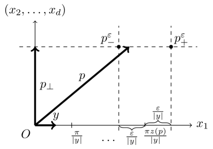
Figure 1: Vectors $p$, $p_{\bot}$, $y$ and $p_{\pm}^{\varepsilon}$ of formula (3.17)

3.2 Approximate reconstruction of phased scattering data

We consider Problem 1 for $d\geq 2$, $L=2$, with the unknown potential $v$ satisfying (1.1b) and with the background potentials $w_{1}$, $w_{2}$ satisfying (1.5). Let

$$D_{\text{ext}}=D\cup\Omega_{1}\cup\Omega_{2},$$ (3.19)

where $D$, $\Omega_{1}$, $\Omega_{2}$ are the domains in (1.1b) and (1.5).

Let $v^{*}_{E}$ be an approximation to $v$ satisfying (2.12) for some $A>0$, $\alpha\geq 0$, $K>0$ and for $E^{*}=E^{*}(K,D_{\text{ext}})$, where $E^{*}(K,D_{\text{ext}})$ is defined according to (2.13). In addition, we suppose that

$$\|v+w_{l}\|_{L^{\infty}(\mathbb{R}^{d})}\leq K,\;\|v^{*}(\cdot,E)+w_{l}\|_{L^{\infty}(\mathbb{R}^{d})}\leq K,\;E\geq E^{*},\;l=1,2.$$ (3.20)

Using the scattering amplitudes $f^{*}_{E}$, $f^{*}_{E,1}$, and $f^{*}_{E,2}$ of the known potentials $v^{*}_{E}$, $v^{*}_{E,1}:=v^{*}_{E}+w_{1}$, and $v^{*}_{E,2}:=v^{*}_{E}+w_{2}$, respectively, and the phaseless scattering data $S$ of Problem 1, we construct an approximation $\widetilde{f}_{E}^{\text{appr}}(p)$ to $(\Phi f_{E})(p)$ for $|p|\leq 2\sqrt{E}$ by the function in Algorithm 1 as follows:

$$\widetilde{f}_{E}^{\text{appr}}(p):=\mathrm{Urec}\left(\Phi f^{*}_{E,1}(p)-\Phi f^{*}_{E}(p),\Phi f^{*}_{E,2}(p)-\Phi f^{*}_{E}(p),\Phi|f_{E}|^{2}(p),\Phi|f_{E,1}|^{2}(p),\Phi|f_{E,2}|^{2}(p)\right)$$ (3.21)

Note that $\widetilde{f}_{E}^{\text{appr}}(p)$ is well defined if

$$\zeta^{*}(p,E):=\det\begin{pmatrix}\mathop{\mathrm{Re}}(\Phi f^{*}_{E,1}(p)-\Phi f^{*}_{E}(p))&\mathop{\mathrm{Im}}(\Phi f^{*}_{E,1}(p)-\Phi f^{*}_{E}(p))\\ \mathop{\mathrm{Re}}(\Phi f^{*}_{E,2}(p)-\Phi f^{*}_{E}(p))&\mathop{\mathrm{Im}}(\Phi f^{*}_{E,2}(p)-\Phi f^{*}_{E}(p))\end{pmatrix}\neq 0.$$ (3.22)

Note that condition (3.22) is satisfied for sufficiently large $E$ at fixed $p\in\mathcal{B}^{d}_{2\sqrt{E}}$ if $\zeta_{\widehat{w}_{1},\widehat{w}_{2}}(p)\neq 0$, where $\zeta_{\widehat{w}_{1},\widehat{w}_{2}}$ is the determinant of formula (3.3). This follows from the estimate

$$\begin{gathered}|\zeta^{*}(p,E)-\zeta_{\widehat{w_{1}},\widehat{w_{2}}}(p)|\leq\mu_{1,\S\ref{sec.isp}}E^{-\frac{1}{2}},\quad p\in\mathcal{B}^{d}_{2\sqrt{E}},\;E\geq E^{*},\end{gathered}$$ (3.23)

where $\mu_{1,\S\ref{sec.isp}}>0$ and $E^{*}=E^{*}(K,D_{\text{ext}})$ is defined according to (2.13), (3.19). Estimate (3.23) follows from the definition of $M$ in Algorithm 1, the formula $M^{-1}=\frac{1}{\zeta}\left(\begin{smallmatrix}\mathop{\mathrm{Im}}W_{2}&-\mathop{\mathrm{Im}}W_{1}\\ -\mathop{\mathrm{Re}}W_{2}&\mathop{\mathrm{Re}}W_{1}\end{smallmatrix}\right)$, and from the estimates

$$\bigl{|}\widehat{v}(p)-\Phi f_{E}(p)\bigr{|} \leq\mu_{2,\S\ref{sec.isp}}E^{-\frac{1}{2}},\quad p\in\mathcal{B}^{d}_{2\sqrt{E}},\;E\geq E^{*},$$ (3.24)

$$\bigl{|}\widehat{v}_{l}(p)-\Phi f_{E,l}(p)\bigr{|} \leq\mu_{2,\S\ref{sec.isp}}E^{-\frac{1}{2}},\quad p\in\mathcal{B}^{d}_{2\sqrt{E}},\;E\geq E^{*},\;l=1,2,$$

where $\mu_{2,\S\ref{sec.isp}}=\mu_{2,\S\ref{sec.isp}}(K,D_{\text{ext}})>0$, $E^{*}=E^{*}(K,D_{\text{ext}})$; see, e.g., [Nov2015en].

Lemma 3.1.

Let $v$, satisfying (1.1b), be the unknown potential of Problem 1 for $d\geq 2$, $L=2$. Let $w_{1}$, $w_{2}$ be the same as in (1.5). Let $v^{*}(\cdot,E)$ be an approximation to $v$, satisfying (2.12) for some $A>0$, $\alpha\geq 0$, $K>0$ and for $E^{*}=E^{*}(K,D_{\text{ext}})$ defined according to (2.13), (3.19). Let $p\in\mathcal{B}^{d}_{2\sqrt{E}}$ be such that

$$|\zeta_{\widehat{w_{1}},\widehat{w_{2}}}(p)|\geq\delta,$$ (3.25)

for some fixed $\delta>0$. Then:

$$|\zeta^{*}(p,E)|\geq\tfrac{\delta}{2},\quad E\geq E^{**},$$ (3.26)

$$\left|\Phi f_{E}(p)-\widetilde{f}_{E}^{\text{appr}}(p)\right|\leq\mu_{3,\S\ref{sec.isp}}\delta^{-1}E^{-\alpha-\frac{1}{2}},\quad E\geq E^{**},$$ (3.27)

$$E^{**}=\max\bigl{(}4\mu_{1,\S\ref{sec.isp}}^{2}\delta^{-2},E^{*}\bigr{)},$$ (3.28)

where $\widetilde{f}_{E}^{\text{appr}}$ is defined by (3.21), $\zeta^{*}$ is defined by (3.22), $\mu_{3,\S\ref{sec.isp}}$ is defined in (LABEL:dis.mu4def) and $\mu_{1,\S\ref{sec.isp}}$ is the constant of (3.23).

Lemma 3.1 is proved in Section LABEL:sec.dis.

The point is that the right-hand side of the estimate in (3.27) decays faster than the right-hand side of the estimate in (2.12b) as $E\to+\infty$. This is a crucial advantage of $\widetilde{f}_{E}^{\text{appr}}$ as an approximation to the unknown phased scattering data $\Phi f_{E}$ in comparison with $\Phi f^{*}_{E}$.

Using Lemma 3.1 we construct the iterative step for phaseless inverse scattering, see Sections 3.3 and 3.4.

3.3 Iterations for background potentials of type A

In this subsection we consider background potentials $w_{1}$, $w_{2}$ satisfying (3.5) and (LABEL:pex.defw).

Iterative step.

We consider Problem 1 for $d\geq 2$, $L=2$, with the unknown potential $v$ satisfying (1.1b) and with the background potentials $w_{1}$, $w_{2}$ satisfying (1.5), (3.5), (LABEL:pex.defw).

Let $v^{*}_{E}$ be an approximation to $v$ satisfying (2.12) for some $A>0$, $\alpha\geq 0$, $K>0$ and $E^{*}=E^{*}(K,D_{\text{ext}})$, where $E^{*}(K,D_{\text{ext}})$ is defined according to (2.13), (3.19) (with $\Omega_{1}=\Omega_{2}$).

We construct an improved approximation $v^{**}_{E}$ to the unknown potential $v$ via the scheme of Section 2.2 with $\Phi f_{E}$ replaced by $\widetilde{f}_{E}^{\text{appr}}$ of formula (3.21) of Section 3.2. Put

$$\begin{gathered}U^{**}_{E}(p)=\widetilde{f}_{E}^{\text{appr}}(p)-\Phi f^{*}_{E}(p)+\widehat{v}^{*}_{E}(p),\\ p\in\mathcal{B}^{d}_{2\sqrt{E}},\;\zeta^{*}(p,E)\neq 0,\end{gathered}$$ (3.29)

where $f^{*}_{E}$ is the scattering amplitude of $v^{*}_{E}$, and $\zeta^{*}$ is defined in (3.22).

Under assumptions (3.5), (LABEL:pex.defw), the iterative step for phaseless inverse scattering is realized as follows.

Theorem 3.2.

Let $v$ satisfy (1.1b) and $v\in W^{n,1}(\mathbb{R}^{d})$ for some $n>d$. Let $w_{1}$, $w_{2}$ be the same as in (1.5), (3.5), (LABEL:pex.defw). Let $v^{*}_{E}$ be an approximation to $v$ satisfying (2.12) for some $A>0$, $\alpha\geq 0$, $K>0$ and for $E^{*}=E^{*}(K,D_{\text{ext}})$, where $E^{*}(K,D_{\text{ext}})$ is defined according to (2.13), (3.19) (with $\Omega_{1}=\Omega_{2}$). We suppose also that

$$\alpha<\tfrac{n-d}{2(d+2\sigma)},$$ (3.30)

where $\sigma$ is the constant of (LABEL:pex.defw). Let

$$\begin{gathered}v^{**}_{E}(x):=\begin{cases}\int_{\mathcal{B}^{d}_{r(E)}}e^{-ipx}U^{**}_{E}(p)\,dp,&x\in D,\\ 0,&x\not\in D,\end{cases}\qquad\mbox{where }r(E):=2\tau E^{\frac{\beta}{n-d}}\mbox{ and }\beta:=\tfrac{(\frac{1}{2}+\alpha)(n-d)}{n+2\sigma}\end{gathered}$$ (3.31)

for some $\tau\in(0,1]$. Here $U^{**}_{E}$ is defined in (3.29), and $\mathcal{B}^{d}_{r}$ is defined by (2.3).

Then there exist constants $B_{1}=B_{1}(\tau,\|v\|_{n,1},A,K,D_{\text{ext}},d,\sigma,n,\mu_{1,\S\ref{sec.pex}})$ and $E_{1}=E_{1}(\tau,\alpha,A,K,D,d,\sigma,n,\mu_{1,\S\ref{sec.pex}})$ defined in (LABEL:tcp.v**est) such that

$$\begin{gathered}\|v^{**}_{E}-v\|_{L^{\infty}(D)}\leq B_{1}E^{-\beta}\qquad\mbox{for all }E\geq E_{1}.\end{gathered}$$ (3.32)

Remark 3.3.

Under assumptions of Theorem 3.2, $v^{**}_{E}(x)$ is well-defined for $E\geq E_{1}$, i.e.:

$$\begin{gathered}\zeta^{*}(p,E)\neq 0\quad\text{for $p\in\mathcal{B}^{d}_{r(E)}$, $E\geq E_{1}$},\\ r(E)\leq 2\sqrt{E}\quad\text{for $E\geq E_{1}$}.\end{gathered}$$ (3.33)

Remark 3.4.

The following three conditions are equivalent:

$$\alpha<\tfrac{n-d}{2(d+2\sigma)},\quad\beta<\tfrac{n-d}{2(d+2\sigma)},\quad\alpha<\beta,$$ (3.34)

where $\beta$ is defined in (3.31), $n>d$, $\alpha>0$, and $\sigma>d$.

Theorem 3.2 is proved in Section LABEL:sec.tcp.

Theorem 3.2 of the present work can be considered as an extension of Theorem 1 of [Agal2016b] to the case when $v^{*}\neq 0$. However, Theorem 3.2 of the present work for $v^{*}=0$ does not coincide with Theorem 1 of [Agal2016b].

Iterations

Let $v$, $w_{1}$, $w_{2}$ satisfy the assumptions of Theorem 3.2. Let $u^{(1)}_{E}=v^{**}_{E}$ for $v^{*}=0$. Note that $u^{(1)}_{E}$ is similar but does not coincide with the approximate reconstruction of Theorem 1 of [Agal2016b]; see formulas (3.12), (3.11) of the present work. In particular, we have that

$$\begin{gathered}\|u^{(1)}_{E}-v\|_{L^{\infty}(D)}=\mathcal{O}(E^{-\alpha_{1}}),\quad E\to+\infty\mbox{ with }\alpha_{1}:=\tfrac{1}{2}\tfrac{n-d}{n+2\sigma}.\end{gathered}$$ (3.35)

Then, applying the iterative step described above in this subsection we construct nonlinear approximate reconstructions $u^{(j)}_{E}$, $j\geq 2$, such that

$$\begin{gathered}\|u^{(j)}_{E}-v\|_{L^{\infty}(D)}=\mathcal{O}(E^{-\alpha_{j}}),\qquad E\to+\infty\mbox{ with }\alpha_{j}:=\tfrac{1}{2}\tfrac{n-d}{d+2\sigma}\bigl{(}1-\bigl{(}\tfrac{n-d}{n+2\sigma}\bigr{)}^{j}\bigr{)}.\end{gathered}$$ (3.36)

The approximations $u^{(j)}_{E}$ of (3.36) for phaseless inverse scattering under assumptions (3.5), (LABEL:pex.defw) are analogs of approximations $u^{(j)}_{E}$ of (2.9) for phased inverse scattering. In a similar way with (2.10),

$$\begin{array}[]{ll}\alpha_{j}\to\alpha_{\infty}=\tfrac{1}{2}\tfrac{n-d}{d+2\sigma}&\text{as $j\to+\infty$},\\ \alpha_{j}\to\tfrac{j}{2}&\text{as $n\to+\infty$},\\ \alpha_{\infty}\to+\infty&\text{as $n\to+\infty$},\end{array}$$ (3.37)

so that the convergence in (3.36) as $E\to+\infty$ is much more optimal then the convergence in (3.12), at least, for large $j$, $n$.

3.4 Iterations for background potentials of type B

In this subsection we consider Problem 1 for $d\geq 2$ with shifted background potentials $w_{1}$, $w_{2}$ described by (LABEL:pex.defw), and (3.8) and unknown potential $v$ satisfying (1.1b).

Iterative step.

We consider the set $Z^{\varepsilon}_{y}$ of formula (3.10). Put

$$\begin{gathered}p^{\varepsilon}(p_{\bot},z,t)=p_{\bot}+\pi z\tfrac{y}{|y|^{2}}+t\varepsilon\tfrac{y}{|y|^{2}},\\ p_{\bot}\in\mathbb{R}^{d},\;p_{\bot}\cdot y=0,\quad z\in\mathbb{Z},\quad t\in\mathbb{R}.\end{gathered}$$ (3.38)

Note that

$$\begin{gathered}\text{for any $p\in Z^{\varepsilon}_{y}$ there exists the unique triple $(p_{\bot},z,t)$ such that}\\ p^{\varepsilon}(p_{\bot},z,t)=p,\;p_{\bot}\in\mathbb{R}^{d},\;p_{\bot}\cdot y=0,\;z\in\mathbb{Z},\;t\in(-1,1).\end{gathered}$$ (3.39)

In addition to $U^{**}$ of (3.29), we also define

$$U^{**}_{N,\varepsilon}(p^{\varepsilon}(p_{\bot},z,t),E)=\sum_{-N\leq j\leq N,j\neq 0}U^{**}\bigl{(}p^{\varepsilon}(p_{\bot},z,j\bigr{)},E)L_{j}(t),$$ (3.40)

under the assumptions that

$$\varepsilon<\tfrac{\pi}{N+1},\;|p^{\varepsilon}(p_{\bot},z,t)|\leq 2\sqrt{E}-\tfrac{\pi}{|y|},\;t\in(-1,1),\;\varepsilon>0,\;N\geq 1,$$ (3.41)

where

$$L_{j}(t)=\frac{(-1)^{N-j}j(t+j)}{(N-j)!(N+j)!}\prod_{1\leq i\leq N,i\neq j}(t^{2}-i^{2}),\quad j=\pm 1,\dots,\pm N.$$ (3.42)

Note that for fixed $p_{\bot}\in\mathbb{R}^{d}$, $p_{\bot}\cdot y=0$, and for fixed $z\in\mathbb{Z}$, function $U^{**}_{N,\varepsilon}(p^{\varepsilon}(p_{\bot},z,t),E)$ is the Lagrange interpolating polynomial of degree $2N-1$ in $t\in\mathbb{R}$ for $U^{**}(p^{\varepsilon}(p_{\bot},z,t),E)$ with the nodes at $t=\pm 1$, …, $\pm N$. In addition, $L_{j}(t)$ is the $j$-th elementary Lagrange interpolating polynomial of degree $2N-1$:

$$L_{j}(t)=\begin{cases}1,&t=j,\\ 0,&t=\pm 1,\dots,\pm N,\;t\neq j.\end{cases}$$ (3.43)

Note also that if assumptions (3.41) are valid for some $p_{\bot}\in\mathbb{R}^{d}$, $p_{\bot}\cdot y=0$, $z\in\mathbb{Z}$, $t\in(-1,1)$, then

$$p^{\varepsilon}(p_{\bot},z,s)\in\mathcal{B}^{d}_{2\sqrt{E}}\setminus Z^{\varepsilon}_{y}\quad\text{for all $s\in[-N,-1]\cup[1,N]$}.$$ (3.44)

Under assumptions (LABEL:pex.defw), (3.8), the iterative step is realized as follows.

Theorem 3.5.

Let $v$ satisfy (1.1b) and $v\in W^{n,1}(\mathbb{R}^{d})$ for some $n>d$. Let $w_{1}$, $w_{2}$ be the same as in (1.5), (LABEL:pex.defw), (3.8). Let $v^{*}_{E}$ be an approximation to $v$ satisfying (2.12a), (2.12) for some $A>0$, $\alpha\geq 0$, $K>0$ and for $E^{*}=E^{*}(K,D_{\text{ext}})$, where $E^{*}(K,D_{\text{ext}})$ is defined according to (2.13), (3.19) (with $\Omega_{1}=\Omega_{2}$). We suppose also that

$$\alpha<\tfrac{n-d}{2(d+2\sigma+\frac{n-d}{2N+1})}\quad\text{for some $N\geq 1$},$$ (3.45)

where $\sigma$ is the constant of (LABEL:pex.defw). Let

$$v^{**}_{E}(x):=\begin{cases}\int\limits_{\mathcal{B}^{d}_{r(E)}\setminus Z^{\varepsilon(E)}_{y}}e^{-ipx}U^{**}_{E}(p)\,dp+,\int\limits_{\mathcal{B}^{d}_{r(E)}\cap Z^{\varepsilon(E)}_{y}}e^{-ipx}U^{**}_{N,\varepsilon(E)}(p,E)\,dp&x\in D\\ 0,&x\notin D\end{cases}$$ (3.46)

$$\mbox{with }r(E)=2\tau E^{\frac{\beta}{n-d}},\quad\varepsilon(E)=E^{-\frac{\beta}{2N+1}},\quad\beta={\tfrac{(\frac{1}{2}+\alpha)(n-d)}{n+2\sigma+\tfrac{n-d}{2N+1}}},\quad\text{for some $\tau\in(0,1]$},$$

where $U^{**}_{E}$ is defined by formulas (3.29); $U^{**}_{N,\varepsilon}(p,E)$ is defined by (3.40); $\mathcal{B}^{d}_{r}$, $Z^{\varepsilon}_{y}$ are defined by (2.3), (3.10).

Then the following estimate holds:

$$\begin{gathered}\|v^{**}_{E}-v\|_{L^{\infty}(D)}\leq B_{2}E^{-\beta},\quad\;E\geq E_{2},\end{gathered}$$ (3.47)

where $B_{2}=B_{2}(\tau,y,N,\|v\|_{n,1},A,K,D_{\text{ext}},d,\sigma,n,\mu_{1,\S\ref{sec.pex}})$ and $E_{2}=E_{2}(\tau,y,\alpha,N,A,K,D,d,\sigma,n,\mu_{1,\S\ref{sec.pex}})$ are defined in (LABEL:trp.B2E2def).

Theorem 3.5 is proved in Section LABEL:sec.trp.

Remark 3.6.

Under assumptions of Theorem 3.5, $v_{E,1}^{**}(x)$ and $v_{E,2}^{**}(x)$ are well-defined for $E\geq E_{2}$, i.e.:

$$\begin{gathered}\zeta^{*}(p,E)\neq 0\quad\text{for $p\in\mathcal{B}^{d}_{r(E)}\setminus Z^{\varepsilon(E)}_{y}$, $\quad E\geq E_{2}$},\\ r(E)\leq 2\sqrt{E}\quad\text{for $E\geq E_{2}$},\end{gathered}$$ (3.48)

where $\zeta^{*}$ is defined by (3.22), and also

$$\varepsilon(E)<\tfrac{\pi}{N+1},\quad|p|\leq 2\sqrt{E}-\tfrac{\pi}{|y|}\quad\text{for $p\in\mathcal{B}^{d}_{r(E)}$, $E\geq E_{2}$}.$$ (3.49)

Remark 3.7.

The following three conditions are equivalent:

$$\alpha<\tfrac{n-d}{2(d+2\sigma+\frac{n-d}{4N+1})},\quad\beta<\tfrac{n-d}{2(d+2\sigma+\frac{n-d}{4N+1})},\quad\alpha<\beta,$$ (3.50)

where $\beta$ is defined in (3.46), $n>d$, $\alpha>0$, and $\sigma>d$. In addition, each of conditions (3.50) is equivalent to the following pair of conditions:

$$\alpha<\tfrac{n-d}{2(d+2\sigma)},\quad N>\tfrac{1}{2}\left(\alpha^{-1}-\bigl{(}\tfrac{n-d}{2(d+2\sigma)}\bigr{)}^{-1}\right)^{-1}-\tfrac{1}{4}.$$ (3.51)

Iterations.

Let $v$, $w_{1}$, $w_{2}$ satisfy the assumptions of Theorem 3.5. Let $u^{(1)}_{E}=v^{**}_{E}$ for $v^{*}=0$. Note that $u^{(1)}_{E}$ is similar, but does not coincide with the approximate reconstruction of Theorem 2 of [Agal2016b]; see formulas (3.18), (3.13) of the present article. In particular, we have that

$$\begin{gathered}\|u^{(1)}_{E}-v\|_{L^{\infty}(D)}+\mathcal{O}(E^{-\alpha_{1}}),\qquad E\to+\infty\quad\mbox{with }\alpha_{1}=\tfrac{1}{2}\tfrac{n-d}{n+2\sigma+\tfrac{n-d}{2N+1}}.\end{gathered}$$ (3.52)

Then, applying the iterative step described above in this subsection we construct nonlinear approximate reconstructions $u_{E}^{(j)}$, $j\geq 2$, such that

$$\begin{gathered}\|u_{E}^{j}-v\|_{L^{\infty}(D)}=\mathcal{O}(E^{-\alpha_{j}})\quad E\to+\infty\quad\mbox{with }\alpha_{j}=\tfrac{1}{2}\tfrac{n-d}{d+2\sigma+\tfrac{n-d}{2N+1}}\biggl{(}1-\biggl{(}\tfrac{n-d}{n+2\sigma+\tfrac{n-d}{2N+1}}\biggr{)}^{j}\biggr{)}.\end{gathered}$$ (3.53)

These approximations $u^{(j)}$ for phaseless inverse scattering under assumptions (LABEL:pex.defw), (3.8) are analogs of approximations $u^{(j)}$ of (2.9) for phased inverse scattering. In a similar way with (2.10) and (3.37),

$$\begin{array}[]{ll}\alpha_{j}\to\alpha_{\infty}=\tfrac{1}{2}\tfrac{n-d}{d+2\sigma+\tfrac{n-d}{2N+1}}&\text{as $j\to+\infty$},\\ \alpha_{j}\to\tfrac{j}{2}&\text{as $n\to+\infty$, $N\to+\infty$},\\ \alpha_{\infty}\to+\infty&\text{as $n\to+\infty$},\end{array}$$ (3.54)

so that the convergence in (3.53) as $E\to+\infty$ is much faster then the convergence in (3.18), at least, for large $j$, $n$, $N$.

4 Numerical experiments

4.1 Implementation of the Fourier transform and its inverse

The iterative algorithm presented in sections 3.3, 3.4 is implemented in Matlab in the two-dimensional case. In our implementation we represent potentials $v$ and $w_{l}$ by discrete functions $\underline{v}$, $\underline{w}_{l}$ defined on the space-variable grid

$$\Gamma^{\rm s}:=\left\{\tfrac{2}{N}(n_{1},n_{2}):n_{1},n_{2}\in\mathbb{Z}_{N}\right\}\mbox{ for }N\in 2\mathbb{N},N\geq\tfrac{2\sqrt{E}}{\pi}$$ (4.1)

$$\text{where }\mathbb{Z}_{N}:=\bigl{\{}-\tfrac{N}{2},-\tfrac{N}{2}+1,\dots,\tfrac{N}{2}-1\bigr{\}}.$$

In turn, the input data $|f(k,l)|^{2}$, $|f_{l}(k,l)|^{2}$ are measured on a grid

$$\mathcal{M}_{E}^{\rm m}=\{(k_{m},l_{m}):m=1..M\}\subset\mathcal{M}_{E},$$

whose precise form depends on the experimental setup. This leads to the following grid in Fourier space:

$$\Gamma^{\rm m}:=\{k_{m}-l_{m}:m=1..M\}$$

Minimal data.

To approximate the inverse Fourier transform of a function, which is supported on $\mathcal{B}^{2}_{2\sqrt{E}}$ and sampled on the grid $\Gamma^{\rm m}$, by the Fast Fourier transform (FFT), $\Gamma^{\rm m}$ has to be rectangular. If $\Gamma^{\rm s}$ is given by (4.1), a minimal choice of $\Gamma^{\rm m}$ is

$$\Gamma^{\rm m}_{\rm min}:=\mathcal{B}^{2}_{2\sqrt{E}}\cap\pi\mathbb{Z}^{2}.$$ (4.2)

A corresponding measurement grid $\mathcal{M}_{E,\rm min}^{\rm m}$ can be defined as in (2.4) replacing $\mathcal{B}^{2}_{2\sqrt{E}}$ by $\Gamma^{\rm m}_{\rm min}$. Extending a function given on $\Gamma^{\rm m}$ to the exterior grid

$$\Gamma^{\rm e}:=\{\pi(n_{1},n_{2}):n_{1},n_{2}\in\mathbb{Z}_{N},\pi^{2}(n_{1}^{2}+n_{2}^{2})>4E\}$$ (4.3)

by $0$, we can compute an approximation to the inverse Fourier transform on $\Gamma^{\rm s}$ by FFT.

Discrete Ewald circles.

The above choice $\Gamma^{\rm m}_{\rm min}$ of the set of measurement points is inconvenient both from an experimental and from a computational point of view since each point in $\Gamma^{\rm m}_{\rm min}$ corresponds to a different incident wave. If a scattering experiment is performed for some incident wave or if the solution to the scattering problem is computed numerically, the resulting far field pattern can be evaluated at other points without essential additional costs.

Therefore, we now consider input data for $M_{1}$ uniformly distributed incident wave vectors $k$ where each far field pattern is evaluated at $M_{2}$ uniformly distributed scattered wave vectors $l$:

$$\begin{gathered}k(s):=\sqrt{E}\bigl{(}\cos(2\pi\tfrac{s}{M_{1}}),\sin(2\pi\tfrac{s}{M_{1}})\bigr{)},\\ l(s,t):=\sqrt{E}\bigl{(}\cos(\tfrac{2\pi s}{M_{1}}+\tfrac{2\pi t}{M_{2}}),\sin(\tfrac{2\pi s}{M_{1}}+\tfrac{2\pi t}{M_{2}})\bigr{)},\end{gathered}\quad s\in\mathbb{Z}_{M_{1}},\;t\in\mathbb{Z}_{M_{2}},$$ (4.4)

resulting in

$$\mathcal{M}_{E,M_{1},M_{2}}^{\rm m}:=\bigl{\{}(k(s),l(s,t))\mid s\in\mathbb{Z}_{M_{1}},t\in\mathbb{Z}_{M_{2}}\bigr{\}},\quad M=M_{1}M_{2},$$ (4.5)

$$\Gamma^{\rm m}_{M_{1},M_{2}}:=\{k-l\colon(k,l)\in\mathcal{M}_{E,M_{1},M_{2}}^{\rm m}\}.$$ (4.6)

This is illustrated in Fig. 2: The points of $\Gamma^{\rm m}=\Gamma^{\rm m}_{M_{1},M_{2}}$ corresponding to a given incident wave vector $k$ are located on the red circle passing through the origin $O$ and centered at point $O^{\prime}$ such that $\overrightarrow{OO^{\prime}}=k$. These points of $\Gamma^{\rm m}$ corresponding to a fixed $k$ are also called (discrete) Ewald circle in the physical literature.

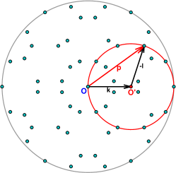
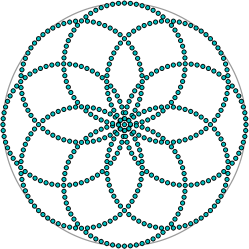
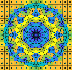
$M_{1}=6$, $M_{2}=10$	$M_{1}=8$, $M_{2}=64$	$M_{1}=8$, $M_{2}=30$

Figure 2: Illustration of sets of transformed measurement points $\Gamma^{\rm m}_{M_{1},M_{2}}$ on Discrete Ewald circles for different values of the numbers $M_{1}$ of incident waves and far field points $M_{2}$. The right panel shows the Voronoi diagram corresponding to the grid $\Gamma^{\rm e}\cup\Gamma^{\rm m}_{M_{1},M_{2}}$. The color is related to the area of a cell.

Given a discrete function $\underline{v}\colon\Gamma^{s}\to\mathbb{C}$ representing a function $v\colon\mathbb{R}^{2}\to\mathbb{C}$, the Fourier transform of $v$ can be approximately represented by a discrete function $\underline{\widehat{v}}\colon\Gamma^{m}\cup\Gamma^{e}\to\mathbb{C}$ such that $\underline{\widehat{v}}=A\underline{v}$, where

$$A:=\left[(N\pi)^{-2}\exp(ix\cdot p)\right]_{p\in\Gamma^{\rm m}\cup\Gamma^{\rm e},x\in\Gamma^{\rm s}}.$$

Here it is necessary to include the points in $\Gamma^{\rm e}$ to obtain small condition numbers of $A$ since the inverse Fourier transform is computed by numerically inverting $A$. Matrix-vector products with $A$ and $A^{*}$ can be computed efficiently without the need to set up and store the matrix $A$ using the Nonequispaced Fast Fourier Transform (NFFT). In our work we use the NFFT implementation of [keiner2009using]. The definitions of the grids $\Gamma^{\rm s}$, $\Gamma^{\rm m}$, $\Gamma^{\rm e}$ and of the Fourier transform matrix $A$ are summarized in Algorithm 2.

data: spatial grid: $\Gamma^{\rm s}:=\{\frac{2}{N}(n_{1},n_{2}):n_{1},n_{2}\in\mathbb{Z},-\frac{N}{2}\leq n_{1},n_{2}<\frac{N}{2}\}$ with $N\in 2\mathbb{N}$, $N\geq\frac{2\sqrt{E}}{\pi}$
measurement points: $\mathcal{M}_{E}^{\rm m}=\{(k_{m},l_{m}):m=1..M\}\subset\mathcal{M}_{E}$
results: Fourier space grids inside and outside $\mathcal{B}^{2}_{2\sqrt{E}}$: $\Gamma^{\rm m}$, $\Gamma^{\rm e}$
matrix representing Fourier transform: $A$
pushforward matrix from the measurement grid $\mathcal{M}^{m}_{E}$ to the Fourier space grid $\Gamma^{m}$: $\Phi$

$\Gamma^{\rm m}:=\{k_{m}-l_{m}:m=1..M\}$; $\triangleright$ grid inside $\mathcal{B}^{2}_{2\sqrt{E}}$

$\Gamma^{\rm e}:=\{\pi(n_{1},n_{2}):n_{1},n_{2}\in\mathbb{Z},-\frac{N}{2}\leq n_{1},n_{2}<\frac{N}{2},\pi^{2}(n_{1}^{2}+n_{2}^{2})>4E\}$; $\triangleright$ grid outside $\mathcal{B}^{2}_{2\sqrt{E}}$

$A:=\left[(\pi N)^{-2}\exp(ix\cdot p)\right]_{p\in\Gamma^{\rm m}\cup\Gamma^{\rm e},x\in\Gamma^{\rm s}}$; $\triangleright$ avoid computation of $A$ and use NFFT instead

$(\Phi\underline{f})_{p}:=\frac{1}{\#(M_{p})}\sum_{m\in M_{p}}\underline{f}_{m}$ where $M_{p}:=\{m:k_{m}-l_{m}=p\}$

Algorithm 2 function [$\Gamma^{\rm m},\Gamma^{\rm e},A,\Phi]=\texttt{fourier\_setup}(\Gamma^{\rm s},\mathcal{M}_{E}^{\rm m})$