Automatic Rank Selection for High-Speed Convolutional Neural Network

Abstract

Low-rank decomposition plays a central role in accelerating convolutional neural network (CNN), and the rank of decomposed kernel-tensor is a key parameter that determines the complexity and accuracy of a neural network. In this paper, we define rank selection as a combinatorial optimization problem and propose a methodology to minimize network complexity while maintaining the desired accuracy. Combinatorial optimization is not feasible due to search space limitations. To restrict the search space and obtain the optimal rank, we define the space constraint parameters with a boundary condition. We also propose a linearly-approximated accuracy function to predict the fine-tuned accuracy of the optimized CNN model during the cost reduction. Experimental results on AlexNet and VGG-16 show that the proposed rank selection algorithm satisfies the accuracy constraint. Our method combined with truncated-SVD outperforms state-of-the-art methods in terms of inference and training time at almost the same accuracy.

1 Introduction

Convolutional Neural Networks (CNN) have been applied to the speech and vision-related tasks and have shown impressive performance. To achieve higher accuracy more complex deep neural network architectures are required, resulting in more computational power and memory. Such demands on compute power and memory makes it difficult to deploy CNNs to resource-constrained systems such as mobile and embedded devices.

There have been many parameter optimization techniques for reducing memory usage and accelerating CNNs including low-rank decomposition [1, 2, 3, 4, 5], channel pruning[6], parameter pruning [7, 8] and quantization [9, 10]. While pruning and quantization techniques can significantly reduce the parameter size and memory usage, it is hard to improve the practical inference runtime on commercial deep-learning platforms. They require special implementations such as sparse computation and low-precision libraries. To directly accelerate the inference work, methods in [1, 2, 3, 4, 5] exploit low-rank decomposition where the convolutional and fully-connected layers are split into the low-complexity layers. X. Zhang et al. [5] and Y. He et al. [6] combine their parameter optimization techniques with Jaderberg et al.’s [2] low-rank decomposition approach to further improve the accuracy.

In low-rank decomposition, the rank is the key parameter that determines the complexity of each layer. In other words, it is directly related to the memory usage, runtime and accuracy. Also, as discussed in [5], rank selection has critical effect on the classification accuracy to carefully select the rank of all layers. Y-D Kim et al. [3] exploit the global analytic solution of Variational Bayesian Matrix Factorization (VBMF) [11] as a toolchain to determine the rank of each layer, and X. Zhang et al. [5] propose a layer-wise greedy strategy to determine the ranks of all layers satisfying the target complexity. This strategy assumes that the classification accuracy is roughly linear to the Principal Component Analysis (PCA) energy and defines an objective function to maximize the accumulated energy subject to the time complexity constraint.

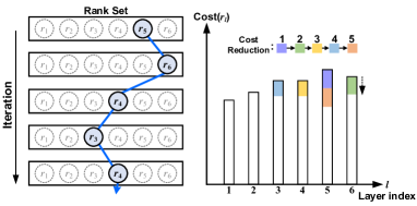
(a) layer-wise search

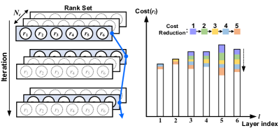
(b) model-wise search

Figure 1: Rank selection strategy (with six kernel layers in a neural network as an example). (a) Legacy layer-wise greedy search selects a layer to reduce the rank for each iteration. (b) Proposed model-wise search selects a rank set to reduce the rank of all layers for each iteration. $N_{c}$ is the number of candidate rank sets.

While these approaches can find the rank for each layer, the layer-wise greedy search [5] is likely to be stuck in a local optima. As shown in Fig. 1(a), to reduce the network complexity (e.g., the number of operations or parameters) the layer-wise greedy algorithm reduces the rank of a layer at a time and selects a best layer maximizing the performance of network model over each iteration. This layer-wise greedy algorithm always does not chooses an immediate worst-affected layer, so that it can prevent to find the best overall solution later.

On the other hand, the proposed model-wise greedy algorithm illustrated in Fig. 1(b) changes the rank of all layers at a time and iteratively selects a best set of rank for all kernel layers (i.e. rank set) maximizing the performance of the network. In this strategy, the performances of some candidate rank sets are compared to select a rank set including the immediate worst-affected layer. This allows to find a relatively optimal solution, since the candidate rank sets are composed of various combinations of the rank. However, the search space will significantly increase, unless the range of the ranks to be search is restricted. For practical implementations, the candidate rank sets have to remain within a reasonable number as an exhaustive search over all rank sets will be computationally out-of-bounds.

To address the above issues, we define rank selection as a combinatorial optimization problem and propose a method for model-wise rank selection with a space rejection rule. In our rank selection algorithm, we search a rank set achieving target accuracy and minimizing the computational cost. We define an accuracy function to estimate the desired final accuracy during cost reduction without fine-tuning. We empirically observe that the test accuracy before fine-tuning (i.e. after low-rank decomposition) is almost linear to the recovered accuracy after several training epochs. From this observation, the accuracy thresholds are determined and used as a termination condition of optimization algorithm and space rejection constraint. Also, we define a cost function, which includes the rank of each layer and then generate the candidate rank sets that make almost same amount of reduction cost. Since the cost function is linear and multidimensional, a huge amount of solution vectors (i.e. rank set) can exist. To effectively find the optimal solution from the search space, we define space rejection parameters. This process is repeated iteratively until the target accuracy is achieved.

In summary, our main contributions are as follows. (1) We propose a model-wise rank selection algorithm constrained on the desired accuracy. (2) We define the linear function of test accuracy before and after fine-tuning. (3) The constraint parameters for the effective search space are defined to obtain an optimal solution. (4) We validate the performance of the proposed algorithm with state-of-the-art on the popular models such as VGG-16 and AlexNet. We show that the proposed optimal rank selection with Jaderberg et al., decomposition method [2] can provide outstanding performance when compared to recent studies [3, 4, 5, 6] for accelerating deep networks. Furthermore, we expect the proposed rank selection algorithm can be effectively applied with not only the basic SVD but also state-of-the-art decomposition algorithms  [5, 6].

2 Low-Rank Decomposition for DNN

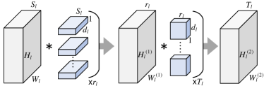
(a) spatial dimension

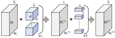
(b) channel dimension

Figure 2: 2-level low-rank decomposition on (a) spatial dimension with ($d_{l}\times 1$), ($1\times d_{l}$) filter window, (b) channel dimension with ($d_{l}\times d_{l}$), ($1\times 1$) filter window

In CNNs, the convolutional layer has a 4-dimensional kernel tensor $\mathcal{K}\in\mathbb{R}^{d\times d\times S\times T}$, where $d$ is the spatial filter window size, $S$ is the number of input channels and $T$ is the number of output channels. By using low-rank decomposition, the 4-dimensional kernel tensor $\mathcal{K}$ can be decomposed into the matrix-multiplication of several small tensors with low-rank subspaces.

We choose truncated singular value decomposition (SVD) for low-rank decomposition such that the tensor $\mathcal{K}$ of the $l$-th convolutional layer can be reshaped to the matrix $K\in\mathbb{R}^{d_{l}S_{l}\times d_{l}T_{l}}$. In a low-rank subspace, the matrix $K$ can be decomposed into $K^{(1)}K^{(2)}$ , where $K^{(1)}\in\mathbb{R}^{d_{l}S_{l}\times r_{l}}$ and $K^{(2)}\in\mathbb{R}^{r_{l}\times d_{l}T_{l}}$ with rank-$r_{l}$ [2].

Fig 2(a) illustrates two decomposed kernel tensors for the $l$-th convolutional layer. Two matrices , $K^{(1)}$ and $K^{(2)}$, are reshaped to 4-dimensional tensors with separate $d_{l}\times 1$ and $1\times d_{l}$ filter windows. The rank of the $l$-th layer $r_{l}$ can be implemented as the number of filters whose sizes are $d_{l}\times 1\times S_{l}$. Fig. 2(b) shows the case of separate $d_{l}\times d_{l}$ and $1\times 1$ filter windows [1]. In this case, matrix $K$ $\in$ $\mathbb{R}^{d^{2}_{l}S_{l}\times T_{l}}$ and the decomposed matrices $K^{(1)}$ $\in$ $\mathbb{R}^{d^{2}_{l}S_{l}\times r_{l}}$ and $K^{(2)}$ $\in$ $\mathbb{R}^{r_{l}\times T_{l}}$.

The original convolutional layer requires $d_{l}^{2}S_{l}T_{l}$ parameters and $d_{l}^{2}S_{l}T_{l}H_{l}W_{l}$ operations. From the spatial decomposition of $l$-th convolutional layer in Fig. 2(a), the number of parameters $p_{l}$ and operations $c_{l}$ are

$$p_{l}=d_{l}r_{l}(S_{l}+T_{l})$$ (1)

$$c_{l}=r_{l}d_{l}(S_{l}W_{l}^{(1)}H_{l}^{(1)}+T_{l}W_{l}^{(2)}H_{l}^{(2)}).$$ (2)

To decompose a fully-connected layer, the shape of filter window $d_{l}$ is fixed to 1.

In this paper, we restrict the number of parameters in the decomposed kernel tensors to less than or equal to the original 4-dimensional tensor. Under this restriction, the maximum rank of each layer is given by

$$r_{l}^{max}=\lfloor S_{l}T_{l}d_{l}/(S_{l}+T_{l})\rfloor.$$ (3)

In Eq. (1), the number of parameters is only controlled by the rank $r_{l}$ as $S_{l}$, $T_{l}$ and $d_{l}$ are constant values in a CNN model. Therefore, the rank of each layer can be adjusted to reduce the complexity of neural network.

3 Approach : Rank Selection

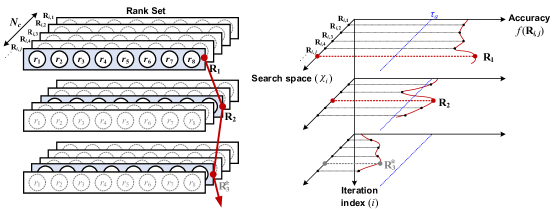
(a) Rank Selection

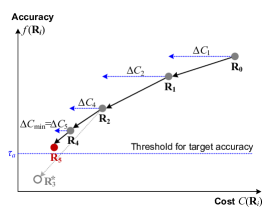
(b) Cost Reduction

Figure 3: Two types of view for iterative rank selection. Every iteration, (a) a rank set maximizing accuracy is selected among $N_{c}$ candidate sets, and (b) the cost is reduced until the accuracy is close to $\tau_{a}$

The goal of proposed algorithm is to search a rank set R minimizing the cost $C(\textbf{R})$ such that the accuracy $f(\textbf{R})$ is greater than a threshold $\tau_{a}$ as shown in Fig. 3,

$$\operatorname*{arg\,min}_{\textbf{R}}C(\textbf{R}),\quad\text{s.t.}\;f(\textbf{R})>\tau_{a},$$ (4)

where a rank set consists of the rank of each layer as $\textbf{R}=\{r_{1},r_{2},...,r_{l}\}$.

The rank selection algorithm repeatedly applies the following four steps: 1) generating the candidate rank sets to achieve a smaller cost, 2) reducing the rank of kernel layers by using the candidate rank sets, 3) scoring the accuracy of each rank set, and 4) selecting a rank set maximizing the accuracy and satisfying an accuracy threshold. After each iteration, a selected rank set is updated as an initial condition.

3.1 Cost Function

The cost function is the linear combination of the rank set with a scalar coefficient, i.e.,

$$C_{m}(\textbf{R})=\sum\limits_{l=1}^{L}p_{l}r_{l},\;\;C_{r}(\textbf{R})=\sum\limits_{l=1}^{L}c_{l}r_{l},$$ (5)

where the $l$ is the index of kernel layer, $L$ is the number of optimized kernel layers in a CNN model. The number of parameters $p_{l}$ and the number of operations $c_{l}$ represent the memory usage and runtime for the rank set R, respectively. Depending on the optimization type such as memory reduction or reducing runtime, $C_{m}(\textbf{R})$ or $C_{r}(\textbf{R})$ is used as the cost function $C(\textbf{R})$ in Eq. (4).

We can also configure the number of optimized layers $L$ to simplify the rank selection algorithm. For the runtime optimization, only convolutional layers are optimized in general [2, 5, 6]. For example, all 5 convolutional layers of AlexNet account for 91.9% of the total number of operations. Note that the 2 fully-connected layers of AlexNet are primarily optimized for the memory usage, as these account for 96.2% of the total number of parameters.

3.2 Accuracy Constraints

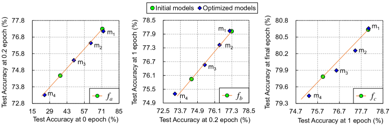
Figure 4: AlexNet top-5 accuracy at 0, 0.2, 1, final training epochs up to 48 epochs (in our implementation). The blue points in graph are the measured accuracy of optimized CNN models having different cost. The green points are initial models to make the linear accuracy function before optimization. For each graph, the accuracy of different training epochs is almost linear

In order to confirm whether the selected rank set satisfies the target accuracy, a fine-tuning ($i.e$ training) stage is required. Calculating the fine-tuned accuracy over every iteration will result in the selection algorithm taking too much time. To this end, we propose approximating the accuracy function to roughly predict the fine-tuned accuracy during optimization.

We have experimentally observed that the test accuracy (top-5) before fine-tuning is almost linear to the fine-tuned test accuracy at the different training epochs, as shown in Fig. 4. We define each accuracy function as linear equation by:

$$f_{a}=\alpha_{a}x+\beta_{a},\;\,f_{b}=\alpha_{b}f_{a}+\beta_{b},\;\,f_{c}=\alpha_{c}f_{b}+\beta_{c},$$ (6)

where $x$ is the accuracy after optimization (0 epoch) and $f_{a}(x),f_{b}(f_{a}),f_{c}(f_{b})$ are accuracy functions for different training epochs.

From the previous observation, we define three types of accuracy thresholds, $\tau_{a},\tau_{b},\tau_{c}$, to satisfy the target accuracy $\mu^{*}$ as

$$f_{a}(\tau_{a})=\tau_{b},\quad f_{b}(\tau_{b})=\tau_{c},\quad f_{c}(\tau_{c})=\mu^{*}.$$ (7)

If we define the accuracy function by training as many optimized models as possible up to the final epoch, the accuracy function will be more accurate and it can precisely estimate the final accuracy without $\tau_{b}$ and $\tau_{c}$. However, to reduce training time and eliminate the latency during optimization due to the accuracy function, we use two initial models such as maximum-cost and half-cost models before the optimization process.

Since the initial models are not from the rank optimization, the estimated accuracy from initial models can be different from the measured accuracy of optimized model. Especially the accuracy at the 0 epoch (i.e. without fine-tuning) is directly affected by the optimization performance. In other words, the threshold $\tau_{a}$ can have some uncertainty. Therefore, we use the accuracy thresholds $\tau_{b}$ and $\tau_{c}$ to confirm that the last selected model satisfies target accuracy $\mu^{*}$. The threshold $\tau_{c}$ at 1 epoch is more reliable than $\tau_{b}$ at 0.2 epoch, since more training data is required to use $\tau_{c}$. Nevertheless, we also use $\tau_{b}$ for early termination of the fine-tuning process before $\tau_{c}$ when the fine-tuned accuracy does not satisfy the threshold.

3.3 Search Space Definition

In our rank selection problem, the search space is defined by all possible combinations of elements in the vector spaces for rank. From the Cartesian product of vector spaces, the total search space $\mathcal{X}$ is defined as:

$$\mathcal{X}=\prod\limits_{l=1}^{L}X_{l}=\{\{r_{1},...,r_{L}\}=\textbf{R}:r_{l}\in X_{l}\},$$ (8)

where $r_{l}$ is the element of vector space $X_{l}$ for rank in $l$-th kernel layer and $r_{l}\geq 0$ for ${\forall}r_{l}\in\mathbb{Z}$. Each subset of $\mathcal{X}$ is a rank set $\textbf{R}=\{r_{l}\}_{l=1}^{L}$.

Space constraints are important to derive the optimal solution, since the search space without any constraints is an infinite field. In this section, we define the parameters for appropriate search space with : 1) upper and lower boundaries of rank, 2) step interval size of elements in vector space, 3) cost variance for iterative cost reduction, 4) cost margin to limit the amount of candidate rank sets.

3.3.1 Boundary Condition

As illustrated in Fig. 5(a), the vector space $X_{l}$ includes the available rank elements for each kernel layer. To restrict $X_{l}$, we set the upper boundary $r^{max}_{l}$ and lower boundary $r^{min}_{l}$, and the interval size $s_{l}$ of respective elements. The proposed model-wise search selects a rank set over each iteration, and a selected rank set $\textbf{R}_{i}=\{r_{l}^{i}\}_{l=1}^{L}$ is updated as the new maximum rank as

$$r^{max}_{l,i}=\begin{cases}r_{l}^{max}&\text{if{~{}}}i=0\\ r_{l}^{i-1}&\text{otherwise}\end{cases},$$ (9)

where $i$ denotes the iteration index and $r_{l}^{max}$ is initial maximum rank in Eq. (3). The range of each $X_{l}$ gets smaller with every iteration. The interval size of elements in $X_{l}$ is $s_{l}=\max(1,\;\lfloor\delta_{s}r_{l}^{max}\rfloor)$. Also, we define the minimum rank of each layer $r_{l}^{min}$ as a product of scaling factor $\delta_{m}$ as

$$r^{min}_{l}=\lceil\delta_{m}r_{l}^{max}\rceil.$$ (10)

We empirically set the scaling factors, $\delta_{s}$ and $\delta_{m}$, to 0.01 and 0.1, respectively, thereby $\delta_{s}$ is 1% of $r_{l}^{max}$ and $\delta_{m}$ is 10% of $r_{l}^{max}$ in our implementation.

From the above results, we define the restricted vector space $X_{l}$ for rank by:

$$X_{l}=\{r_{l}|\,r_{l}=n\,s_{l},\;r_{l}^{min}\leq r_{l}\leq r_{l,i}^{max}\},$$ (11)

where $n\in\mathbb{Z}$ and $r_{l}$ is the integer multiple of $s_{l}$ within the upper and lower boundary.

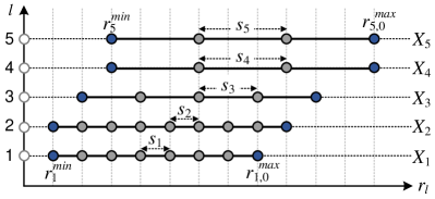
(a) Vector space $X_{l}$ of $r_{l}$

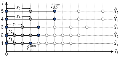
(b) Vector space $\hat{X}_{l}$ of $\hat{r}_{l}$

Figure 5: Vector spaces $X_{l}$ and $\hat{X}_{l}$ of rank in $l$-th kernel layer (show 5 layers as an example). The gray and blue dots are elements of each vector space. Respective elements in a vector space have the $s_{l}$ interval size. (a) Rank $r_{l}$ in $X_{l}$ is element of rank set $\textbf{R}=\{r_{l}\}_{l=1}^{L}$. (b) Rank $\hat{r}_{l}$ in $\hat{X}_{l}$ is element of candidate rank set $\Delta\textbf{R}=\{\hat{r}_{l}\}_{l=1}^{L}$

3.4 Candidate Rank Sets for Cost Reduction

The proposed algorithm reduces the cost of CNN model by cost variance $\Delta C_{i}=|C_{i}-C_{i+1}|$ in every iteration. The initial cost variance is defined by $\Delta C_{0}=\lfloor\delta_{r}\,C_{max}\rfloor$, where $\delta_{r}$ is the cost scaling factor to determine the amount of cost reduction and $C_{max}$ is the maximum cost of the CNN model by applying $\{r_{l}^{max}\}_{l=1}^{L}$ in Eq. (3).

To reduce the rank, we generate the rank sets $\{\Delta\textbf{R}\}$ resulting in $\Delta C_{i}\pm\sigma$, where $\sigma$ is the cost margin. Without $\sigma$, the solution rank set may not exist, since the cost function is a multi-dimensional equation and the rank is an integer under our space limitation. By applying $\sigma$, we can define the reduction space $\mathcal{\hat{X}}_{i}$ satisfying $\Delta C_{i}\pm\sigma$ as:

$$\mathcal{\hat{X}}=\{\Delta\textbf{R}\,|\,\Delta C_{i}-\sigma\leq C(\Delta\textbf{R})\leq\Delta C_{i}+\sigma\}.$$ (12)

We define the set $\Delta\textbf{R}$ in $\mathcal{\hat{X}}$ as the candidate rank set. Also, $\mathcal{\hat{X}}$ can be represented by the Cartesian product of the vector space $\hat{X}_{l}$ for a candidate rank set. As illustrated in Fig. 5(b), $\hat{X}_{l}$ has a maximum rank $\hat{r}_{l}^{max}$ and the interval of elements is same as Fig. 5(a).

$$\hat{X}_{l}=\{\hat{r}_{l}|\,\hat{r}_{l}=n\,s_{l},\;0\leq\hat{r}_{l}\leq\hat{r}_{l,i}^{max}\},$$ (13)

$$\hat{r}^{max}_{l,i}=\lfloor\min(\Delta C_{i}/\epsilon_{l},\;\;2\delta_{r}\,r_{l,i}^{max},\;\;r_{l,i}^{max}-{r}_{l}^{min})\rfloor,$$ (14)

where $\epsilon_{l}$ is the coefficient of cost function in Eq. (4). The type of target cost determines $\epsilon_{l}$ as one of $p_{l}$ or $c_{l}$.

We generate the reduced rank sets $\{\textbf{R}|\,\textbf{R}=\textbf{R}_{i-1}-\Delta\textbf{R},\Delta\textbf{R}\in\mathcal{\hat{X}}\}$ , and choose $\textbf{R}^{*}=\operatorname*{arg\,max}_{\textbf{R}}f(\textbf{R})$. We update $\textbf{R}^{*}$ as $\textbf{R}_{i}$ only for $f({\textbf{R}}^{*})>\tau_{a}$. Otherwise, $\textbf{R}_{i}$ is still $\textbf{R}_{i-1}$ and the cost variance is reduced by:

$$\Delta C_{i+1}=\begin{cases}\lfloor\Delta C_{i}/2\rfloor&\text{if{~{}}}f(\textbf{R}^{*})\leq\tau_{a}\\ \Delta C_{i}&\text{otherwise}\end{cases}.$$ (15)

In detail, we consider that the cost variance is too large to find the optimal solution, and reduce $\Delta C_{i}$ by half.

3.5 Rejection Space

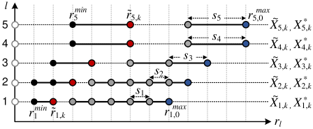
Figure 6: Rejected and retained vector spaces, $\tilde{X}_{l.k}$ and ${X_{l,k}^{*}}$ respectively, for $k$-th rejection rank set $\tilde{R}_{k}$. The black and red dots are in $\tilde{X}_{l,k}$ and the red dot is the rejected rank $\tilde{r}_{l,k}$. The gray and blue dots in ${X}_{l,k}^{*}$ are the remain elements in ${X_{l}}$

To further reduce the space complexity and retain valuable rank sets, we define the rejection space $\tilde{\mathcal{X}}$ and exclude $\tilde{\mathcal{X}}$ from $\mathcal{X}$. The strategy to maximize the probability of selecting the optimal rank set is to eliminate the unnecessary rank sets with the accuracy below $\tau_{a}$.

At every iteration, we categorize the rejection rank sets $\{\tilde{\textbf{R}}|f(\tilde{\textbf{R}})\leq\tau_{a}\}$.In addition to the observed rejection rank set, all smaller rank sets are included in the rejection space, since lower rank size corresponds to lower accuracy. As illustrated in Fig. 6, $X_{l}$ is separated into $\tilde{X}_{l,k}$ and ${X_{l,k}^{*}}$, which are rejected and retained vector spaces, respectively. For $\tilde{\textbf{R}}_{k}\in\{\tilde{\textbf{R}}\}$, we define the vector space $\tilde{X}_{l,k}$ with the observed $\tilde{\textbf{R}}_{k}=\{\tilde{r}_{l,k}\}_{l=1}^{L}$ as the maximum rank by:

$$\tilde{X}_{l,k}=\{r_{l}|\,r_{l}=n\,s_{l},\;r_{l}^{min}\leq r_{l}\leq\tilde{r}_{l,k}\},$$ (16)

where $k$ is the index of rejection rank set. From the Cartesian product of rejection vector space $\tilde{X}_{l,k}$, we can define the rejection subspace $\tilde{\mathcal{X}}_{k}$. The total rejection space $\tilde{\mathcal{X}}$ is the union of all $\tilde{\mathcal{X}}_{k}$,

$$\tilde{\mathcal{X}}_{k}=\prod_{l=1}^{L}\tilde{X}_{l,k},\;\;\;\tilde{\mathcal{X}}=\bigcup\limits_{k=1}^{N_{k}}\tilde{\mathcal{X}_{k}},$$ (17)

where $N_{k}$ is the number of rejection sets in the candidate rank sets. Therefore, we retain the effective search space ${\mathcal{X}}^{*}$ as the complement of $\tilde{\mathcal{X}}$ in ${\mathcal{X}}$ by:

$${\mathcal{X}}^{*}={\mathcal{X}}\cap\tilde{\mathcal{X}}^{\complement}=\{{\textbf{R}}:{\textbf{R}}\in{\mathcal{X}}\;|\;\textbf{R}\notin\tilde{\mathcal{X}}\}.$$ (18)

The remaining rank set in ${\mathcal{X}}^{*}$ will be considered for next iteration search.

3.6 Algorithm Procedure

Algorithm 1 Model-wise Automatic Rank Search

1:// Stage1 : Cost minimization subject to accuracy constraint $\tau_{a}$

2:Initialize the target cost $\epsilon_{l}$, optimization layer $L$, space constraints $\{r_{l}^{max},r_{l}^{min},s_{l}\}$ and reduction cost $\Delta C_{0}$

3:repeat

4:    Update the parameters $\{r^{max}_{l,i},\hat{r}^{max}_{l,i},\Delta C_{i}\}$

5:    Extract $N_{c}$ candidate rank sets $\{\Delta\textbf{R}|(\textbf{R}_{i-1}-\Delta\textbf{R})\notin\tilde{\mathcal{X}}_{i-1}\}$ from reduction space $\hat{\mathcal{X}}_{i}$

6:    for each rank set in $\{\Delta\textbf{R}\}$  do

7:         Check the accuracy $f(\textbf{R})$ from $\textbf{R}=\textbf{R}_{i-1}-\Delta\textbf{R}$

8:         Group the rejection set $\{\tilde{\textbf{R}}|\tilde{\textbf{R}}={\textbf{R}},f(\tilde{\textbf{R}})\leq\tau_{a}\}$

9:    end for

10:    Define the rejection vector spaces $\tilde{X}_{l,k}$ from each rejection set $\tilde{\textbf{R}}_{k}\in\{\tilde{\textbf{R}}\}$

11:    Generate the rejection space $\tilde{\mathcal{X}}_{i}=\tilde{\mathcal{X}}_{i-1}\bigcup_{k}(\prod_{l}{\tilde{X}_{l,k}})$

12:    Select a rank set $\textbf{R}^{*}=\operatorname*{arg\,max}_{\textbf{R}}f(\textbf{R})$

13:    Update the list of selected rank set $[\textbf{R}]\leftarrow\textbf{R}_{i}=\textbf{R}^{*}$ only for $f(\textbf{R}^{*})>\tau_{a}$.

14:      Otherwise, $\textbf{R}_{i}=\textbf{R}_{i-1}$.

15:    $i=i+1$

16:until $f(\textbf{R}^{*})\leq\tau_{a}$ and $\Delta C_{i}\ \leq\Delta C_{min}$

17:

18:// Stage2 : Fine-tuning and accuracy check with threshold $\tau_{b}$ and $\tau_{c}$

19:$\textbf{R}_{j}$ = last updated rank set in $[\textbf{R}]$

20:repeat

21:    Briefly fine-tune the network model using $\textbf{R}_{j}$ till 1 epoch

22:    If $f(\textbf{R}_{j})<\tau_{b}$ or $f(\textbf{R}_{j})<\tau_{c}$     

23:         $j=j+1$

24:         $\textbf{R}_{j}$ = previous updated rank set of $\textbf{R}_{j-1}$ in [R]     

25:until $f(\textbf{R}_{j})\geq\tau_{b}$ and $f(\textbf{R}_{j})\geq\tau_{c}$

26:Fine-tune the network model using the last selected $\textbf{R}_{j}$ for final epoch

27:Output : fine-tuned model using $\textbf{R}_{j}$

The rank search procedure is formalized in Alg. 1. The proposed algorithm aims to iteratively minimize the cost satisfying the target accuracy. At first, the space constraints for boundary condition, $\{r_{l}^{max}$,$r_{l}^{min},s_{l}\}$, are initialized with the scaling factors, $\{\delta_{s},\delta_{m},\delta_{r}\}$, when the target cost and number of optimization layers are determined. At every iteration, the search space is redefined by updating the constraint parameters and removing the unnecessary search space. The candidate rank sets $\Delta\textbf{R}$ are extracted from the search space. For each candidate rank set, the accuracy of the reduced rank set is scored. Then, a rank set $\textbf{R}^{*}$ that provides maximum accuracy is selected, and $\textbf{R}_{i}$ is updated in the list $[\textbf{R}]$ if the accuracy is higher than threshold $\tau_{a}$.This procedure repeats iteratively until the accuracy of $\textbf{R}^{*}$ and the reduction cost $\Delta C_{i}$ are lower than the $\tau_{a}$ and minimum cost reduction $\Delta C_{min}$, respectively.

After cost reduction, we fine-tune a CNN model of the last selected rank set in the list $[\textbf{R}]$ up to 1 epoch.The accuracy at 0.2 epoch and 1 epoch is verified whether it satisfies the threshold $\tau_{b}$ and $\tau_{c}$. When the accuracy condition is not satisfied, we fine-tune another network model with previous updated rank set in $[\textbf{R}]$ and check the accuracy again until all accuracy thresholds are satisfied. Finally, an optimized CNN model using the last selected rank set is fine-tuned for the final epoch.

3.6.1 Optimization Time

There are three parts of the optimization process, which are the generation of candidate rank sets, accuracy check and brief fine-tuning. The most time consuming part is the accuracy check in the cost minimization step (i.e. Step1). The total time of accuracy check is proportional to the number of candidate sets. Therefore, in every iteration we only test the randomly extracted $N_{c}$ sets to maintain a reasonable amount of optimization time. However, the smaller the number of extracted subsets, the lower the probability of obtaining a optimal solution. Therefore, we incrementally reject the rank sets that are predicted to have a lower accuracy by using the method of Sec. 3.2. This space rejection increases the probability of having a near optimal solution with the extracted subset. Also, we set the intermediate accuracy threshold such as $\tau_{b}$ before $\tau_{c}$ for early termination of the fine-tuning stage.

4 Experiments

In our experiments, we use two CNN models: AlexNet [12] and VGG-16 [13]. AlexNet has 5 convolutional layers and 3 fully-connected layers, and VGG-16 has 13 convolutional layers and 3 fully-connected layers. The baseline top-5 accuracy of AlexNet is 80.03% [12] and VGG-16 is 89.9% [13] on the ImageNet 2012 validation set [14] of 1000 classes. In the fine-tuning and evaluation stage, we crop 227x227 size images for AlexNet and 224x224 size images for VGG-16. For fine-tuning VGG-16, the ImageNet dataset is scaled with a fixed smallest side 256 as described in [13]. We use Berkeley’s Caffe [15] for the implementation.

In the first step, we decompose the CNN model by using Denil et al. [1] and Jaderberg et al. methods [2]. For the first convolutional layer, we adopt the 2-level channel decomposition [1] to separate $d\times d$ kernel window into the $d\times d$ and $1\times 1$ windows.Since the input channel size of first layer is small due to the RGB image, the method in [1] is better solution to increase the number of decomposed filters than the method in [2]. For other kernel layers, we adopt the 2-level spatial decomposition [2] to separate $d\times d$ kernel window into the $d\times 1$ and $1\times d$ windows.

For the initialization of rank selection algorithm, we empirically set the minimum rank of each layer $r_{l}^{min}$ to 10% of $r_{l}^{max}$ and the interval size $s_{l}$ of the vector space is 1% of $r_{l}^{max}$ in our implementation. To further speedup the algorithm, we restrict the number of candidate rank sets $N_{c}$ to maximum 200. Also, we use 10% of the validation dataset to check the accuracy for the selection procedure.

4.1 Experiments with AlexNet

We define the the target accuracy and target cost from [3] using tensor decomposition on AlexNet. The cost of AlexNet is minimized until the accuracy is almost same as the balanced optimization approach [3].

4.1.1 Balanced optimization

Table 1: Performance comparison for balanced optimization

AlexNet	FLOPs	Weights	Top-5 Acc.	Target Acc.	Decomp.	Rank Sel.
Y-D Kim [3]	272.0 M ($\times$2.67)	11.0 M (-81.6 %)	78.33%	-	Tucker (3-level)	VBMF [11]
Ours (final model)	238.5 M ($\times$3.04)	10.6 M (-82.6 %)	78.43%	78.33%[3]	SVD (2-level)	Model-wise Rank Search

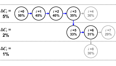
(a) Iterative cost reduction

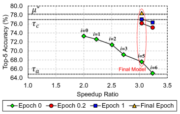
(b) Accuracy of optimized models

Figure 7: AlexNet results for balanced optimization (runtime and memory usage). (a) There are 8 iterations for cost reduction, where $i$ is iteration index and ${\Delta C_{i}}$ is the amount of cost reduction. At the gray circle, the accuracy is lower than the threshold $\tau_{a}$. (b) Final model satisfies all accuracy constraints

To reduce both memory usage and runtime, we set the target cost $\epsilon_{l}$ as the number of operations $c_{l}$ and optimize the whole network including the fully-connected layers. The target accuracy$\mu^{*}$ is 78.33%[3].

Two initial models with the 100% and 50% of total cost are fine-tuned to determine the accuracy threshold from the linear accuracy function in Fig. 7(a). At every iteration, the accuracies of extracted 100 candidate sets are verified without fine-tuning. From the half-cost model, there are 8 iterations for cost reduction, and 5 rank sets are updated in the list $[\textbf{R}]$ by satisfying the accuracy condition $\tau_{a}$. Since the accuracy of optimized models at $i$=(4,7,8) is lower than accuracy threshold $\tau_{a}$, the cost is reduced at the previous model satisfying $\tau_{a}$.

After cost reduction is done, the last optimized model is fine-tuned to verify the accuracy constraints at 0.2 and 1 training epoch. In our experiment, the last model ($i$=7) does not satisfy the accuracy threshold $\tau_{c}$ at 1 training epoch. Therefore, the previous model ($i$=6) is fine-tuned, and it satisfies all accuracy threshold and target accuracy. To recover the accuracy, we set the base learning rate as $10^{-4}$ and decrease it by a factor of 2 every 4 epochs with a batch size of 256 till 32 epochs.

Compared to the combination of Tucker-decomposition [16] and VBMF based rank selection [3], our final model shows 3.04 times speedup and 78.43% accuracy while reducing significant memory usage as denoted in Table. 1.

4.2 Experiments with VGG-16

4.2.1 Runtime optimization

Table 2: Performance comparison. FLOPs is computed including fully-connected layers

VGG-16	FLOPs	Top-5 Acc.	Target Acc.	Decomp.	Rank Sel.
X. Zhang ($\times 3$) [5]	4764 M ($\times$3.26)	89.9%	-	3D: Asym. (3-level)	layer-wise search
Ours (final model)	3837 M ($\times$4.03)	90.0%	89.9%[13]	SVD (2-level)	model-wise rank search

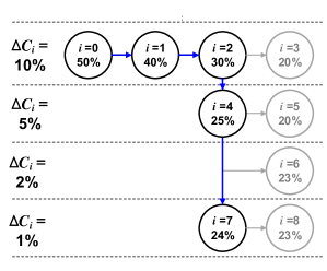
(a) Iterative Cost Reduction

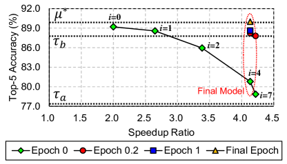
(b) Accuracy of optimized models

Figure 8: VGG-16 result for runtime optimization. (a) There are 8 iterations for cost reduction, where $i$ is iteration index and ${\Delta C_{i}}$ is the amount of cost reduction. At the gray circle, the accuracy is lower than the threshold $\tau_{a}$. (b) Final model satisfies all accuracy constraints

While VGG-16 model has a high top-5 classification accuracy of 89.9%, the weight parameters are highly redundant [5]. To maintain the original accuracy, we optimize the runtime of VGG-16 and compare our optimization results with the recent works [5, 6]. The target accuracy is 89.9% [13].

First, we fine-tune two models with 50% and 25% of the maximum cost to determine the accuracy threshold. From the half-cost model without fine-tuning, the rank selection from 200 candidate sets is repeated for 8 iterations, and 4 rank sets are updated in the list $[\textbf{R}]$ by satisfying the accuracy condition $\tau_{a}$.

The brief fine-tuning of last selected model ($i$=7) is terminated at 0.2 epoch, since the test accuracy is lower than the threshold $\tau_{b}$. Therefore, we fine-tune the previous model ($i$=6), and check the accuracy requirement for all the thresholds. For fine-tuning, we set the base learning rate as $10^{-5}$ and decrease it by a factor of 10 every 4 epochs with a batch size of 16 up to 8 epochs.

Table 3: Performance comparison of state-of-the-art work

Models (VGG-16)	Top-5 Accuracy		Optimization Method
	w/ FT	w/o FT
ADC ($\times 4$)  [17]	-	80.7%	reinforcement learning
Ours ($\times 4.03$)	90.0%	80.8%	rank searching algorithm

Table 4: Comparison of CPU and GPU processing time for forward and backward pass. Forward pass is related to inference and backward pass is related to training. The runtime is for a single view (the performance results are based on our implementation of [5, 6])

Models (VGG-16)	Forward Speed		Backward Speed		Decomposed Kernel Layers
	CPU [ms]	GPU [ms]	CPU [ms]	GPU [ms]
X. Zhang ($\times 3$) [5]	1088.42 ($\times$2.14)	9.98 ($\times$1.14)	1005.15 ($\times$1.87)	14.15 ($\times$1.28)	37 (34 Conv, 3 FC)
Y. He [6] (3C: C-P)	968.31 ($\times$2.40)	8.62 ($\times$1.31)	892.68 ($\times$2.49)	12.94 ($\times$1.40)	37 (34 Conv, 3 FC)
Ours (final model)	824.35 ($\times$2.82)	8.39 ($\times$1.35)	761.24 ($\times$2.92)	12.11 ($\times$1.49)	29 (26 Conv, 3 FC)

Finally, the optimized model shows 90.0% accuracy and achieves a 4.03 times speedup as shown in Table. 2 and Fig. 8(b). Our method using the SVD and model-wise rank selection shows better performance than the combination of asymmetric reconstruction and layer-wise rank selection [5]. Also, the optimization performance of our algorithm is comparable to the state-of-the-art works, ADC [17] for spatial decomposition. We expect the proposed algorithm can be effectively applied to other network acceleration algorithms such as asymmetric reconstruction [5] and channel-pruning [6] to achieve higher accuracy.

4.2.2 Processing Time

We perform the runtime benchmark of optimized models on Nvidia GTX 1080 GPU and Intel Zeon E5-2620 CPU. We use the standard library in Caffe to measure the processing time of forward and backward pass. To fairly compare the precessing time, we implement the CNN models based on the network specification of X. Zhang et al. ($\times 3$) [5] and Y. He et al. [6]. Also, we compare the runtime performance at almost same accuracy, since there is a trade-off between accuracy and computation time. Table. 4 shows the results of GPU and CPU processing times for a single view. Our method uses 2-level decomposition based on truncated SVD , whereas [5, 6] use 3-level spatial and channel decomposition. Therefore, we can implement a shorter CNN model, and it provides faster processing time than [5, 6] in terms of inference (i.e. forward pass) and training (i.e. forward and backward pass).

5 Conclusion

In this paper, we propose a model-wise rank selection algorithm that minimizes the CNN complexity while satisfying the target accuracy. We define the rank selection problem as the combinatorial optimization, and propose the space limitation parameters to reduce the search space and obtain an optimal solution. Also, we define a linearly-approximated accuracy function to predict the recovered accuracy in the rank selection stage. From experiments on AlexNet and VGG-16, we show that the proposed optimal rank selection algorithm successfully satisfies the target accuracy and provides a faster CNN model while maintaining the same accuracy.

References

- [1] Misha Denil, Babak Shakibi, Laurent Dinh, Nando de Freitas, et al. Predicting parameters in deep learning. In Advances in Neural Information Processing Systems (NIPS), pages 2148–2156, 2013.
- [2] Max Jaderberg, Andrea Vedaldi, and Andrew Zisserman. Speeding up convolutional neural networks with low rank expansions. In Proceedings of the British Machine Vision Conference (BMVC). BMVA Press, 2014.
- [3] Yong-Deok Kim, Eunhyeok Park, Sungjoo Yoo, Taelim Choi, Lu Yang, and Dongjun Shin. Compression of deep convolutional neural networks for fast and low power mobile applications. In Proceedings of the International Conference on Learning Representations (ICLR), May 2016.
- [4] Emily L Denton, Wojciech Zaremba, Joan Bruna, Yann LeCun, and Rob Fergus. Exploiting linear structure within convolutional networks for efficient evaluation. In Advances in Neural Information Processing Systems (NIPS), pages 1269–1277, 2014.
- [5] Xiangyu Zhang, Jianhua Zou, Kaiming He, and Jian Sun. Accelerating very deep convolutional networks for classification and detection. IEEE transactions on pattern analysis and machine intelligence, 38(10):1943–1955, 2016.
- [6] Yihui He, Xiangyu Zhang, and Jian Sun. Channel pruning for accelerating very deep neural networks. In The IEEE International Conference on Computer Vision (ICCV), Oct 2017.
- [7] Song Han, Huizi Mao, and William J Dally. Deep compression: Compressing deep neural networks with pruning, trained quantization and huffman coding. In Proceedings of the International Conference on Learning Representations (ICLR), May 2016.
- [8] Song Han, Jeff Pool, John Tran, and William Dally. Learning both weights and connections for efficient neural network. In Advances in Neural Information Processing Systems (NIPS), pages 1135–1143, 2015.
- [9] Yunchao Gong, Liu Liu, Ming Yang, and Lubomir Bourdev. Compressing deep convolutional networks using vector quantization. arXiv preprint arXiv:1412.6115, 2014.
- [10] Matthieu Courbariaux, Yoshua Bengio, and Jean-Pierre David. Binaryconnect: Training deep neural networks with binary weights during propagations. In C. Cortes, N. D. Lawrence, D. D. Lee, M. Sugiyama, and R. Garnett, editors, Advances in Neural Information Processing Systems 28, pages 3123–3131. Curran Associates, Inc., 2015.
- [11] Shinichi Nakajima, Masashi Sugiyama, S Derin Babacan, and Ryota Tomioka. Global analytic solution of fully-observed variational bayesian matrix factorization. Journal of Machine Learning Research, 14(Jan):1–37, 2013.
- [12] Alex Krizhevsky, Ilya Sutskever, and Geoffrey E Hinton. Imagenet classification with deep convolutional neural networks. In F. Pereira, C. J. C. Burges, L. Bottou, and K. Q. Weinberger, editors, Advances in Neural Information Processing Systems 25, pages 1097–1105. Curran Associates, Inc., 2012.
- [13] Karen Simonyan and Andrew Zisserman. Very deep convolutional networks for large-scale image recognition. In Proceedings of the International Conference on Learning Representations (ICLR), May 2015.
- [14] Jia Deng, Wei Dong, Richard Socher, Li-Jia Li, Kai Li, and Li Fei-Fei. Imagenet: A large-scale hierarchical image database. In Computer Vision and Pattern Recognition, 2009. CVPR 2009. IEEE Conference on, pages 248–255. IEEE, 2009.
- [15] Yangqing Jia, Evan Shelhamer, Jeff Donahue, Sergey Karayev, Jonathan Long, Ross Girshick, Sergio Guadarrama, and Trevor Darrell. Caffe: Convolutional architecture for fast feature embedding. In Proceedings of the 22nd ACM international conference on Multimedia, pages 675–678. ACM, 2014.
- [16] Ledyard R Tucker. Some mathematical notes on three-mode factor analysis. Psychometrika, 31(3):279–311, 1966.
- [17] Yihui He and Song Han. ADC: automated deep compression and acceleration with reinforcement learning. CoRR, abs/1802.03494, 2018.