Extreme binary black holes in a physical representation

Abstract

Stationary axisymmetric binary systems of unequal co and counter-rotating extreme Kerr black holes apart by a conical singularity are studied. Both solutions are well identified as two $3$-parametric subfamilies of the Kinnersley-Chitre metric, and fully depicted by Komar parameters: the two masses $M_{1}$ and $M_{2}$, and a coordinate distance $R$, where the angular momenta $J_{1}$ and $J_{2}$ are functions of these parameters. Our physical representation allows us to identify some limits and novel physical properties.

I Introduction

The well-known Kinnersley-Chitre (KCH) $5$-parametric exact solution KCH represents the extreme limit case of the so-called double-Kerr-NUT solution developed by Kramer and Neugebauer in 1980 KramerNeugebauer , which allows to treat the superposition of two massive rotating sources in General Relativity. Both solutions permits us to study the dynamical interaction among two Kerr-type sources in stationary axisymmetric spacetimes by solving properly the corresponding axis conditions. In this respect, Yamazaki Yamazaki found an asymptotically flat special member of the KCH metric through a specific parametrization that vanishes the NUT parameter NUT which is identical to the Tomamitsu-Sato solution with distortion parameter $\delta=2$ TS . A few years ago, after following the ideas provided by Yamazaki Yamazaki to eliminate the NUT parameter, Manko and Ruiz MR solved for the first time in analytical way the axis condition that disconnects the region in between sources, with the main purpose to describe co and counter-rotating binary black hole (BH) systems separated by a conical singularity Bach ; Israel ; i.e, a massless strut related with the interaction force among sources which is a measure of their gravitational attraction as well as the spin-spin interaction. Even though the Manko-Ruiz representation of the KCH metric allows us to clarify some physical aspects related to unequal binary systems, the total Komar Komar mass $M$ and total angular momentum $J$ of the binary BH system contain complicated formulas in terms of dimensionless parameters, which could lead to erroneous interpretations at the moment of assigning numerical values to them. Therefore, it is mandatory to review once again the KCH solution in order to express the metric of two-body systems of unequal co and counter-rotating extreme BHs separated by a strut in a representation with a more physical aspect.

The main goal pursued in this paper is a rederivation of the two 3-parametric subfamilies of the KCH metric concerning to co/counter-rotating BHs considered earlier in MR , but with the principal characteristic that now both solutions will be given in terms of arbitrary physical Komar parameters: the masses $M_{1}$ and $M_{2}$, as well as the coordinate distance $R$. We will obtain some well-known limits of the KCH solution and other dynamical aspects not considered before; in particular, those related to the merging process of interacting BHs. The paper is organized as follows. In Sec. II we describe the KCH exact solution as well as the two approaches considered earlier in Refs. Yamazaki ; MR ; in particular, the path used by Manko and Ruiz to solve the axis conditions in order to describe interacting binary BHs by means of two 3-parametric special members of the KCH metric. Later on, in Sec. III we begin with a new more suitable $5$-parametric representation of the KCH solution with the main objective to solve once again the axis conditions and depict both metrics for interacting BHs in a more realistic physical representation. Concluding remarks can be found in Sec. IV.

II The KCH exact solution

Stationary axisymmetric spacetimes are well defined with the Papapetrou metric Papapetrou

$$ds^{2}=f^{-1}\left[e^{2\gamma}(d\rho^{2}+dz^{2})+\rho^{2}d\varphi^{2}\right]-f(dt-\omega d\varphi)^{2},$$ (1)

and Einstein vacuum field equations can be reduced by means of Ernst’s formalism Ernst into a new complex equation

$$({\cal{E}}+\bar{\cal{E}})({\cal{E}}_{\rho\rho}+\rho^{-1}{\cal{E}}_{\rho}+{\cal{E}}_{zz})=2({\cal{E}}_{\rho}^{2}+{\cal{E}}_{z}^{2}),$$ (2)

where a suffix $\rho$ or $z$ denotes partial differentiation. It follows that one can be able to find the metric functions $f(\rho,z)$, $\omega(\rho,z)$, and $\gamma(\rho,z)$ of the line element Eq. (1) by solving the following equations:

$$\begin{split}f&={\rm{Re}}({\cal{E}}),\\ \omega_{\rho}&=-4\rho({\cal{E}}+\bar{\cal{E}})^{-2}{\rm{Im}}({\cal{E}}_{z}),\qquad\omega_{z}=4\rho({\cal{E}}+\bar{\cal{E}})^{-2}{\rm{Im}}({\cal{E}}_{\rho}),\\ \gamma_{\rho}&=\rho({\cal{E}}+\bar{\cal{E}})^{-2}\left({\cal{E}}_{\rho}\bar{\cal{E}}_{\rho}-{\cal{E}}_{z}\bar{\cal{E}}_{z}\right),\qquad\gamma_{z}=2\rho({\cal{E}}+\bar{\cal{E}})^{-2}\rm{Re}({\cal{E}}_{\rho}\,{\bar{\cal{E}}}_{z}),\end{split}$$ (3)

once we know an analytical solution for the non-linear Eq. (2). In this sense, the KCH solution solves Eq. (2) exactly, it is described by the complex potential ${\cal{E}}$ which is given by^[30]

$$\begin{split}{\cal{E}}&=\frac{\Lambda-2\Gamma}{\Lambda+2\Gamma},\\ \Lambda&=(\alpha^{2}-\beta^{2})(x^{2}-y^{2})^{2}+p^{2}(x^{4}-1)+q^{2}(y^{4}-1)-2i\alpha(x^{2}+y^{2}-2x^{2}y^{2})\\ &-2ipqxy(x^{2}-y^{2})-2i\beta xy(x^{2}+y^{2}-2),\\ \Gamma&=e^{-i\gamma_{o}}[px(x^{2}-1)+iqy(y^{2}-1)-i(p\alpha+iq\beta)x(x^{2}-y^{2})+i(p\beta+iq\alpha)y(x^{2}-y^{2})],\end{split}$$ (4)

where $(x,y)$ are prolate spheroidal coordinates depicted as

$$x=\frac{r_{+}+r_{-}}{2\kappa},\quad y=\frac{r_{+}-r_{-}}{2\kappa},\qquad r_{\pm}=\sqrt{\rho^{2}+(z\pm\kappa)^{2}}.$$ (5)

Is it worthwhile to mention that the above solution Eq. (4) contains the real parameters $p$, $q$, $\gamma_{o}$, $\alpha$, $\beta$, and the half of the separation distance among sources $\kappa$, where the first three obey the constraints

$$p^{2}+q^{2}=1,\qquad|e^{-i\gamma_{o}}|=1.$$ (6)

Taking into account $y=1$ and $x=z/\kappa$, the Ernst potential on the upper part of the symmetry axis adopts the form

$$\begin{split}{\cal{E}}(\rho=0,z)&=\frac{e_{+}(z)}{e_{-}(z)},\\ e_{\pm}(z)&=(p^{2}+\alpha^{2}-\beta^{2})z^{2}\mp 2\kappa[(p+q\beta-ip\alpha)e^{-i\gamma_{o}}\pm i(pq+\beta)]z\\ &+\kappa^{2}(p^{2}-\alpha^{2}+\beta^{2}+2i\alpha)\pm 2\kappa^{2}e^{-i\gamma_{o}}(q\alpha-ip\beta),\end{split}$$ (7)

from which the first Geroch-Hansen multipolar moments Geroch ; Hansen can be explicitly computed once we apply the Fodor-Hoenselaers-Perjés procedure FHP ; they read MR

$$\begin{split}M&=\frac{2\kappa(pP-pQ\alpha+qP\beta)}{p^{2}+\alpha^{2}-\beta^{2}},\qquad J=M\left[\frac{(pq+\beta)M+\kappa(qQ\alpha+pP\beta)}{pP-pQ\alpha+qP\beta}-2J_{0}\right],\\ J_{0}&=-\frac{2\kappa(pQ+pP\alpha+qQ\beta)}{p^{2}+\alpha^{2}-\beta^{2}},\qquad e^{-i\gamma_{o}}:=P-iQ,\end{split}$$ (8)

where $M$ and $J$ represent the total mass and total angular momentum of the system, respectively. Besides, $J_{0}$ is the NUT parameter.^[31] Starting with the previous axis data, in Ref. MR is provided the full KCH metric via the Sibgatullin method Sibgatullin , which is written down in a closed analytical form by using the Perjés’ factor structure Perjes ; it reads

$$\begin{split}f&=\frac{N}{D},\qquad\omega=2J_{0}(y-1)+\frac{\kappa(y^{2}-1)F}{N},\qquad e^{2\gamma}=\frac{N}{K_{0}^{2}(x^{2}-y^{2})^{4}},\\ N&=\mu^{2}+(x^{2}-1)(y^{2}-1)\sigma^{2},\qquad D=N+\mu\pi-(y^{2}-1)\sigma\tau,\qquad F=(x^{2}-1)\sigma\pi+\mu\tau,\\ \mu&=p^{2}(x^{2}-1)^{2}+q^{2}(y^{2}-1)^{2}+(\alpha^{2}-\beta^{2})(x^{2}-y^{2})^{2},\\ \sigma&=2\left[pq(x^{2}-y^{2})+\beta(x^{2}+y^{2})-2\alpha xy\right],\\ \pi&=(4/K_{0})\{K_{0}\left[pPx(x^{2}+1)+2x^{2}+qQy(y^{2}+1)\right]+2(pQ+pP\alpha+qQ\beta)\\ &\times\left[pqy(x^{2}-y^{2})+\beta y(x^{2}+y^{2})-2\alpha xy^{2}\right]-K_{0}(x^{2}-y^{2})\left[(pQ\alpha-qP\beta)x+(qP\alpha-pQ\beta)y\right]\\ &-2(q^{2}\alpha^{2}+p^{2}\beta^{2})(x^{2}-y^{2})+4(pq+\beta)x(\beta x-\alpha y)\},\\ \tau&=(4/K_{0})\{K_{0}x\left[(qQ\alpha+pP\beta)(x^{2}-y^{2})+qP(y^{2}-1)\right]+(pQ+pP\alpha+qQ\beta)y\\ &\times\left[(p^{2}-\alpha^{2}+\beta^{2})(x^{2}-y^{2})+y^{2}-1\right]-pQK_{0}y(x^{2}-1)-2p(q\alpha^{2}-q\beta^{2}-p\beta)(x^{2}-y^{2})\\ &+(pq+\beta)(y^{2}-1)\},\\ K_{0}&=p^{2}+\alpha^{2}-\beta^{2}.\end{split}$$ (9)

One should notice that the above metric is invariant under the change $\{p,q,P,Q,\alpha,\beta\}\rightarrow\{-p,-q,-P,-Q,\alpha,\beta\}$. Bearing in mind that asymptotically flat spacetimes can be obtained from Eq. (9) when the NUT parameter $J_{0}$ is eliminated, there exist several possibilities to achieve such a task. On one hand, Yamazaki Yamazaki proposed the solution

$$P=\frac{p+q\beta}{\sqrt{(p+q\beta)^{2}+p^{2}\alpha^{2}}},\qquad Q=-\frac{p\alpha}{\sqrt{(p+q\beta)^{2}+p^{2}\alpha^{2}}},$$ (10)

while on the other hand Manko and Ruiz MR went beyond at the moment of considering the following solution

$$\alpha=-\frac{Q(p+q\beta)}{pP}.$$ (11)

Due to the fact that the metric function $\omega$ on the middle region among the sources ($x=1$, $y=z/\kappa$), acquires the form

$$\begin{split}&q\alpha\left[QK_{0}-(2p+P)\alpha\right]+\beta\left[pPK_{0}+(2p+P)q\beta-1+2p^{2}\right]-pq(1+pP)\\ &-(pQ+pP\alpha+qQ\beta)(q^{2}+\alpha^{2}-\beta^{2})=0,\end{split}$$ (12)

one notices that Yamazaki’s approach does not simplify the above condition, while the second proposal considered by Manko and Ruiz factorizes it as follows

$$\left[(p^{2}-Q^{2})\beta^{2}-pq(1+pP+Q^{2})\beta-p^{2}(1+pP)\right]\left[(p^{2}-Q^{2})\beta-pq(pP+Q^{2})\right]=0,$$ (13)

which eventually may lead us to the description of two-body systems of unequal co/counter-rotating BHs separated by a massless strut by choosing the first/second factor respectively. In this direction, over all the parametrization of MR , the total mass $M$ and total angular momentum $J$ of the system were given in terms of dimensionless parameters $\{p,q,P,Q\}$, therefore, the analysis of the dynamics for such BH systems was mostly performed in a numerical way. For instance, the total mass $M$ and total angular momentum $J$ in the counter-rotating sector are obtainable from the second factor of Eq. (13) in combination with Eq. (11); they assume the form

$$M=\frac{2\kappa(pP+q^{2})}{p^{2}-q^{2}},\qquad J=\frac{2\kappa^{2}q\left[(1+2pP)^{2}-(p+P)^{2}\right]}{p(p^{2}-q^{2})^{2}}.$$ (14)

To make matters worse, the situation is even much more complicated in the co-rotating sector, where after using the first factor of Eq. (13) together with Eq. (11) one obtains

$$\begin{split}M&=\frac{\kappa\left[\pm q\Delta_{o}-p(1+p^{2})-q^{2}P\right]}{p(p^{2}-q^{2})},\\ J&=\frac{\kappa M}{2p(p^{2}-q^{2})}\{\pm\Delta_{o}(2p^{2}P-2p-P)+2q(1+p^{2}+pP)-qP(p^{2}-q^{2})(p-P)\},\\ \Delta_{o}&:=\sqrt{4p^{2}(1+pP)+q^{2}(p+P)^{2}}.\end{split}$$ (15)

This last point naturally motivates the present work to consider another more suitable parametrization which might invert the problem and establish a real physical representation of the KCH metric to describe interacting BHs in a more transparent form.

III Extreme binary black holes in a physical representation

The problem of expressing the KCH metric with a more physical aspect can be tackled by adopting first a new representation for such a solution. In order to do so, we begin with a new suitable parametrization of the Ernst potential on the symmetry axis

$$\begin{split}&e(z)=\frac{z^{2}-[M+i(\mathfrak{q}+2J_{0})]z+\frac{2\Delta-R^{2}}{4}+\frac{\mathfrak{q}(P_{1}+P_{2})}{2M}-2\mathfrak{q}J_{0}+i\left(P_{1}-\frac{2J_{0}(P_{2}+M\mathfrak{q})}{\mathfrak{q}}\right)}{z^{2}+(M-i\mathfrak{q})z+\frac{2\Delta-R^{2}}{4}-\frac{\mathfrak{q}(P_{1}+P_{2})}{2M}+iP_{2}},\\ \Delta:=M^{2}-\mathfrak{q}^{2},\end{split}$$ (16)

where the KCH solution contains now the five parameters $\{M,\mathfrak{q},R,P_{1},P_{2}\}$ related to the set $\{p,q,\gamma_{o},\alpha,\beta,\kappa\}$ via the expressions

$$\begin{split}\mathfrak{q}&=\frac{2\kappa[p(q+Q)+pP\alpha+(1+qQ)\beta]}{p^{2}+\alpha^{2}-\beta^{2}},\qquad R=2\kappa,\\ P_{1}&=\frac{2\kappa^{2}[(1-qQ)\alpha-pP\beta]}{p^{2}+\alpha^{2}-\beta^{2}}+2\left(M+\frac{P_{2}}{\mathfrak{q}}\right)J_{0},\qquad P_{2}=\frac{2\kappa^{2}[(1+qQ)\alpha+pP\beta]}{p^{2}+\alpha^{2}-\beta^{2}},\end{split}$$ (17)

being $M$ and $J_{0}$ expressed lines up. The inverse relation among these two sets of parameters is completed if we construct once again the full KCH metric by using the Perjés’ factor structure in the same way like in Ref. MR , leading us to

$$\begin{split}p&=\frac{M(\alpha_{+}\beta_{+}-\alpha_{-}\beta_{-})}{\sqrt{(\alpha_{+}^{2}+M^{2}\beta_{-}^{2})(\alpha_{-}^{2}+M^{2}\beta_{+}^{2})}},\qquad q=-\frac{\alpha_{+}\alpha_{-}+M^{2}\beta_{+}\beta_{-}}{\sqrt{(\alpha_{+}^{2}+M^{2}\beta_{-}^{2})(\alpha_{-}^{2}+M^{2}\beta_{+}^{2})}},\\ P&=\frac{M(\alpha_{+}\beta_{+}+\alpha_{-}\beta_{-})}{\sqrt{(\alpha_{+}^{2}+M^{2}\beta_{-}^{2})(\alpha_{-}^{2}+M^{2}\beta_{+}^{2})}},\qquad Q=\frac{\alpha_{+}\alpha_{-}-M^{2}\beta_{+}\beta_{-}}{\sqrt{(\alpha_{+}^{2}+M^{2}\beta_{-}^{2})(\alpha_{-}^{2}+M^{2}\beta_{+}^{2})}},\\ \alpha&=MR\left(\frac{[\mathfrak{q}\alpha_{+}+M(R+M)\beta_{-}][q_{o}-2M^{2}R(\alpha_{-}-\mathfrak{q}\beta_{+})]-[\mathfrak{q}\alpha_{-}-M(R-M)\beta_{+}][q_{o}+2M^{2}R(\alpha_{+}-\mathfrak{q}\beta_{-})]}{(\alpha_{-}^{2}+M^{2}\beta_{+}^{2})(\alpha_{+}^{2}+M^{2}\beta_{-}^{2})}\right),\\ \beta&=MR\left(\frac{[\mathfrak{q}\alpha_{+}+M(R+M)\beta_{-}][q_{o}-2M^{2}R(\alpha_{-}-\mathfrak{q}\beta_{+})]+[\mathfrak{q}\alpha_{-}-M(R-M)\beta_{+}][q_{o}+2M^{2}R(\alpha_{+}-\mathfrak{q}\beta_{-})]}{(\alpha_{-}^{2}+M^{2}\beta_{+}^{2})(\alpha_{+}^{2}+M^{2}\beta_{-}^{2})}\right),\\ \kappa&=R/2,\qquad q_{o}:=\alpha_{+}\alpha_{-}+M^{2}\beta_{+}\beta_{-},\qquad\alpha_{\pm}:=M(\Delta\pm MR)-\mathfrak{q}(P_{1}+P_{2}),\qquad\beta_{\pm}:=2P_{2}\pm\mathfrak{q}R.\end{split}$$ (18)

Additionally, the total angular momentum $J$ as well as the NUT charge $J_{0}$, in this new representation are reduced to

$$\begin{split}J&=M\mathfrak{q}-\frac{P_{1}-P_{2}}{2}+\frac{J_{0}P_{2}}{\mathfrak{q}},\\ J_{0}&=\frac{\mathfrak{q}}{2M}\left(\frac{\mathfrak{q}^{2}(P_{1}+P_{2})^{2}-M^{2}\left[4P_{1}P_{2}-\Delta(R^{2}-\Delta)\right]}{\mathfrak{q}^{2}\left[M(R^{2}-\Delta)+\mathfrak{q}(2P_{1}+2P_{2}+M\mathfrak{q})\right]-M(2P_{2}+M\mathfrak{q})^{2}}\right).\end{split}$$ (19)

With the main purpose of describing the interaction among two extreme BHs separated by a conical singularity Bach ; Israel , the first equation that eliminates $J_{0}$ is

$$\mathfrak{q}^{2}(P_{1}+P_{2})^{2}-M^{2}\left[4P_{1}P_{2}-\Delta(R^{2}-\Delta)\right]=0,$$ (20)

while after developing a few non-trivial calculations one gets a simple quadratic expression for the axis condition $\omega(x=1,y=2z/R)=0$, that disconnects the region in between sources, namely

$$\begin{split}\mathfrak{q}\left[M^{2}(R^{2}+MR+\mathfrak{q}^{2})(P_{1}-P_{2})^{2}+(\Delta+MR)(\Delta-MR-R^{2})(P_{1}+P_{2})^{2}\right]&\\ -M^{2}(R^{2}-\Delta)\left\{\left[M\mathfrak{q}^{2}+(R+M)(R^{2}+MR+\mathfrak{q}^{2})\right](P_{1}-P_{2})-M\mathfrak{q}(R+M)(R^{2}-\Delta)\right\}=0,&\end{split}$$ (21)

and it is not complicated to show that Eqs. (20) and (LABEL:conditionmiddle) contain a trivial set of solutions, which explicitly are

$$\begin{split}P_{1,2}&=\frac{\mp\Delta[R^{2}+MR+\mathfrak{q}^{2}]+\epsilon M\sqrt{\Delta(R^{2}+MR+\mathfrak{q}^{2})^{2}+M^{2}\mathfrak{q}^{2}(R^{2}-\Delta)}}{2M\mathfrak{q}},\\ P_{1,2}&=\frac{\mp\mathfrak{q}\Delta+\epsilon M\sqrt{(R+M)^{2}(R^{2}-\Delta)+\mathfrak{q}^{2}\Delta}}{2(R+M)},\qquad\epsilon=\pm 1,\\ \end{split}$$ (22)

where the subindexes $1$ and $2$ are associated with $-$ and $+$ signs, while the sign of $\epsilon$ refers to the location of the sources. In what follows in this paper we are going to use $\epsilon=1$; this means that the first/second source will be located up/down, respectively. The aforementioned Eq. (LABEL:solutions) is giving us two $3$-parametric subfamilies of the KCH metric that we are going to explore in the next subsections. It is worth mentioning that Eq. (LABEL:conditionmiddle) has been derived recently in Ref. Cabrera for the case of non-extreme sources.

III.1 Co-rotating binary black holes

Using the first solution of Eq. (LABEL:solutions) it can be possible to describe a co-rotating two-body system of unequal Kerr sources separated by a massless strut, as a $3$-parametric subclass of the KCH metric. By means of Perjes’s representation Perjes , the Ernst potential ${\cal{E}}$ and the full metric are depicted by

$$\begin{split}{\cal{E}}&=\frac{\Lambda-2\Gamma}{\Lambda+2\Gamma},\qquad f=\frac{N}{D},\qquad\omega=\frac{R(y^{2}-1)F}{2N},\qquad e^{2\gamma}=\frac{N}{\mathfrak{q}^{4}R^{4}(x^{2}-y^{2})^{4}},\\ \Lambda&=\mathfrak{q}^{2}(R^{2}-\Delta)(x^{2}-y^{2})^{2}+\Delta[\mathfrak{q}^{2}(x^{4}-1)+(R+M)^{2}(y^{4}-1)]\\ &+2i\mathfrak{q}\left\{xy\left[\Delta(R+M)(x^{2}-y^{2})-M(MR+\Delta)(x^{2}+y^{2}-2)\right]-\delta_{1}(x^{2}+y^{2}-2x^{2}y^{2})\right\},\\ \Gamma&=\left(\frac{\mathfrak{q}(\Delta-MR-R^{2})+i\delta_{1}}{MR[(R+M)^{2}+\mathfrak{q}^{2}]}\right)\{\Delta\left[(R+M)^{2}+\mathfrak{q}^{2}\right]\left[\mathfrak{q}x(x^{2}-1)-i(R+M)y(y^{2}-1)\right]\\ &-\mathfrak{q}\left\{M(\Delta+MR)\left[(R+M)x-iqy\right]-\delta_{1}\left[(R+M)y-i\mathfrak{q}x\right]\right\}(x^{2}-y^{2})\},\\ N&=\mu^{2}+(x^{2}-1)(y^{2}-1)\sigma^{2},\quad D=N+\mu\pi-(1-y^{2})\sigma\tau,\quad F=(x^{2}-1)\sigma\pi-\mu\tau,\\ \mu&=\mathfrak{q}^{2}(R^{2}-\Delta)(x^{2}-y^{2})^{2}+\Delta\left[\mathfrak{q}^{2}(x^{2}-1)^{2}+(R+M)^{2}(y^{2}-1)^{2}\right],\\ \sigma&=2\mathfrak{q}\left\{\mathfrak{q}^{2}Rx^{2}+\left[2M(\Delta+MR)-\mathfrak{q}^{2}R\right]y^{2}-2\delta_{1}xy\right\},\\ \pi&=\left(\frac{4}{MR}\right)\{\mathfrak{q}^{2}x\left[M^{2}R\left(R(x^{2}-y^{2})+2Mx\right)+\Delta(\Delta-MR-R^{2})(1+y^{2})-4M\delta_{1}y\right]\\ &+y\left[2M\left(\Delta(R+2M)(R^{2}+\mathfrak{q}^{2})+M^{4}R\right)y+\delta_{1}\left(M(\Delta+MR)(1+y^{2})-\mathfrak{q}^{2}R(1+x^{2})\right)\right]\},\\ \tau&=\left(\frac{4\mathfrak{q}\Delta}{MR}\right)\{-x\left[(R^{2}+MR+\mathfrak{q}^{2})(Rx+2M)x+(R+M)(\Delta-MR-R^{2})\right]\\ &+(1-x)y\left[M(R^{2}-\Delta)y+\delta_{1}(1+x)\right]+M\left((R+M)^{2}+\mathfrak{q}^{2}\right)\}\\ \delta_{1}&:=\epsilon\sqrt{\Delta(R^{2}+MR+\mathfrak{q}^{2})^{2}+M^{2}\mathfrak{q}^{2}(R^{2}-\Delta)}.\end{split}$$ (23)

It is feasible to prove from Eq. (18) that the above metric is obtainable from the KCH metric KCH ; MR after doing the following changes in the real parameters:

$$\begin{split}p&=\frac{\mathfrak{q}}{\sqrt{(R+M)^{2}+\mathfrak{q}^{2}}},\qquad q=-\frac{R+M}{\sqrt{(R+M)^{2}+\mathfrak{q}^{2}}},\qquad e^{-i\gamma_{o}}=\frac{\mathfrak{q}(\Delta-MR-R^{2})+i\delta_{1}}{MR\sqrt{(R+M)^{2}+\mathfrak{q}^{2}}},\\ \alpha&=\frac{\mathfrak{q}\delta_{1}}{\Delta\left[(R+M)^{2}+\mathfrak{q}^{2}\right]},\qquad\beta=\frac{M\mathfrak{q}(\Delta+MR)}{\Delta\left[(R+M)^{2}+\mathfrak{q}^{2}\right]}.\end{split}$$ (24)

On the other hand, the Komar integrals Komar for each mass and angular momentum can be calculated through the Tomimatsu’s formulae Tomimatsu0 :

$$M_{i}=-\frac{1}{8\pi}\int_{H_{i}}\omega\,{\rm{Im}}({\cal{E}}_{z})d\varphi dz,\qquad J_{i}=-\frac{1}{8\pi}\int_{H_{i}}\omega\,\left(1+\frac{1}{2}\omega\,{\rm{Im}}({\cal{E}}_{z})\right)d\varphi dz,$$ (25)

where the integrals must be evaluated over the corresponding horizon $H_{i}$. Apparently it seems quite complicated to develop such a goal, nevertheless, the technical difficulty of finding the correct formulas for the Komar masses and angular momenta of the sources can be circumvented by taking into account a limit process after expanding the above expressions around the values taken by $x$ and $y$ on the regions surrounding to each BH; for instance, if we are surrounding the upper BH, one can take into the computer code $x=1+\varepsilon,y=1$ in the region on the axis $z>R/2$, for $|\varepsilon|<<1$, but in the region in between $|z|<R/2$ we put now $x=1,y=1-\varepsilon$. A trivial calculation yields the expressions

$$\begin{split}M_{1,2}&=\frac{M}{2}\mp\frac{\delta_{1}}{2(\Delta+MR)},\\ J_{1,2}&=M_{1,2}\left[\frac{\mathfrak{q}}{2}-\frac{\Delta(R+M)(R^{2}+MR+\mathfrak{q}^{2})\pm(\Delta+MR)\delta_{1}}{2M\mathfrak{q}(R^{2}-\Delta)}\right],\end{split}$$ (26)

and it is easy to observe that $M=M_{1}+M_{2}$. Furthermore, the expression $J=J_{1}+J_{2}$ allows us to recover the aforementioned Eq. (19) for the total angular momentum in the absence of the NUT charge, namely

$$J=M\mathfrak{q}-\frac{P_{1}-P_{2}}{2}=M\mathfrak{\mathfrak{q}}+\frac{\Delta(R^{2}+MR+\mathfrak{q}^{2})}{2M\mathfrak{q}},$$ (27)

whereas the difference between the values of the masses yields the relation

$$M_{2}-M_{1}=\frac{\delta_{1}}{\Delta+MR},$$ (28)

and eventually one arrives to a bicubic equation for solving

$$\begin{split}&\mathfrak{q}^{6}+3a_{1}\mathfrak{q}^{4}+3a_{2}\mathfrak{q}^{2}+a_{3}=0,\\ a_{1}&:=(1/3)[2R^{2}+2MR-2M^{2}+(M_{1}-M_{2})^{2}],\\ a_{2}&:=(1/3)(R+M)[(R-M)(R^{2}+2MR-M^{2})-2M(M_{1}-M_{2})^{2}],\\ a_{3}&:=-M^{2}(R+M)^{2}\left[R^{2}-(M_{1}-M_{2})^{2}\right],\end{split}$$ (29)

whose explicit roots are given by

$$\begin{split}\mathfrak{q}^{2}_{(k)}&=-a_{1}+e^{i2\pi k/3}\left[b_{o}+\sqrt{b_{o}^{2}-a_{o}^{3}}\right]^{1/3}+e^{-i2\pi k/3}a_{o}\left[b_{o}+\sqrt{b_{o}^{2}-a_{o}^{3}}\right]^{-1/3},\\ a_{o}&:=a_{1}^{2}-a_{2},\qquad b_{o}:=(1/2)\left[3a_{1}a_{2}-a_{3}-2a_{1}^{3}\right],\quad k=0,1,2.\end{split}$$ (30)

In this particular case we choose $k=0$ since it defines entirely a real parameter $\mathfrak{q}$ which starts and ends at the same value given by the total mass $M$, where the coordinate distance runs from $R=0$ until $R\rightarrow\infty$. The substitution of this real solution into Eq. (26) permits us to demonstrate that during the merging process ($R=0$) each individual angular momentum $J_{i}$ is related to its corresponding mass $M_{i}$ by means of Cabrera

$$\frac{J_{1}}{M_{1}^{2}}=1+\frac{M_{2}}{M_{1}},\qquad\frac{J_{2}}{M_{2}^{2}}=1+\frac{M_{1}}{M_{2}},$$ (31)

where such a process conceives a single extreme BH of mass $M=M_{1}+M_{2}$ and angular momentum $J=J_{1}+J_{2}$, satisfying exactly a well-known formula for extreme BHs Cabrera

$$J=J_{1}+J_{2}=(M_{1}+M_{2})^{2}.$$ (32)

Moreover, when the sources are far away from each other, in the limit $R\rightarrow\infty$ are recovered the simple expressions for extreme BHs, namely

$$\frac{J_{1}}{M_{1}^{2}}=1,\qquad\frac{J_{2}}{M_{2}^{2}}=1.$$ (33)

All these features already mentioned can be noticed in Fig. 1. Regarding now the dynamical aspects of this co-rotating two-body system, the interaction force associated with the strut can be computed straightforwardly by using the formula Israel ; Weinstein , to obtain

$$\mathcal{F}=\frac{1}{4}(e^{-\gamma_{s}}-1)=\frac{\Delta\left[\mathfrak{q}^{2}-(R+M)^{2}\right]}{4\left(\Delta+MR\right)^{2}}\equiv\frac{M_{1}M_{2}[(R+M)^{2}-\mathfrak{q}^{2}]}{(R^{2}-\Delta)[(R+M)^{2}+\mathfrak{q}^{2}]},$$ (34)

where $\gamma_{s}$ is the value of the metric function $\gamma$ evaluated on the region of the conical singularity; i.e., $\gamma(x=1)$. The strut prevents the BHs from falling onto each other; it means that as both horizons are getting closer and closer, the interaction force $\mathcal{F}\rightarrow\infty$. The minimal distance occurs when $R\rightarrow 0$, and for that case $\mathfrak{q}\rightarrow M$ [see Eq. (29) or Fig. 1 (a)]. Let us now assume that the sources move away from each other, thus, in the limit $R\rightarrow\infty$ one gets the following expansion:

$$\mathcal{F}\simeq\frac{M_{1}M_{2}}{R^{2}}\left[1-\frac{2M^{2}}{R^{2}}+\frac{4M(M_{1}^{2}+8M_{1}M_{2}+M_{2}^{2})}{R^{3}}+O\left(\frac{1}{R^{4}}\right)\right],$$ (35)

that matches with the formula already given by Dietz and Hoenselaers DH once we put the condition for extreme co-rotating sources given by Eq. (33). The strut might be removed if we consider $|\mathfrak{q}|=R+M$ in the above formula Eq. (34). Nevertheless, as was demonstrated first by Hoenselaers Hoenselaers , an absence of a strut might produce the appearance of naked singularities (ring singularities) off the axis, since at least one of the two masses will be negative even yet if the total mass of the system does not violate the positive mass theorem SchoenYau1 ; SchoenYau2 . The last statement can be confirmed directly from Eq. (26).

To conclude the subsection, the identical case $M_{1}=M_{2}=m$,  $J_{1}=J_{2}=j$ is recovered when is imposed the condition $\delta_{1}=0$, and is also taken into account a simple redefinition $\mathfrak{q}\rightarrow 2\mathfrak{q}$, thus, one arrives to the extreme condition for identical co-rotating BHs, which was considered earlier in Costa ; CCLP

$$m^{2}-\mathfrak{q}^{2}\left(1-\frac{4m^{2}(R^{2}-4m^{2}+4\mathfrak{q}^{2})}{[R(R+2m)+4\mathfrak{q}^{2}]^{2}}\right)=0,$$ (36)

where it can be shown that such a condition for identical extreme co-rotating BHs leads us to a bicubic equation, which is precisely the identical case of Eq. (29). Furthermore, after replacing such a condition in Eq. (27) [or Eq. (26)], the final expression for the equal angular momentum acquires the form CCLP

$$j=\frac{m\mathfrak{q}[(R+2m)^{2}+4\mathfrak{q}^{2}]}{R(R+2m)+4\mathfrak{q}^{2}}.$$ (37)

For identical constituents, the values for the angular momentum $j$ are contained within the interval $1<j/m^{2}\leq 2$ Costa , while for nonequal sources the ratio $J_{i}/M_{i}^{2}$ can be greater or lower than $2$ [see Eq. (31) or Fig. 1 (b)]. This peculiarity was first pointed in Ref. MR using numerical arguments.

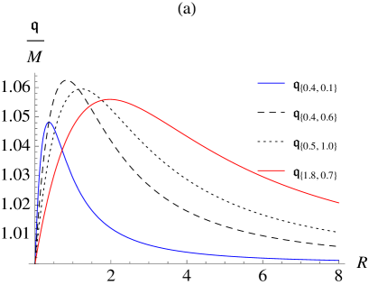
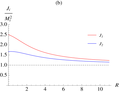
Figure 1: (a) Behavior for the parameter $\mathfrak{q}$ in the co-rotating case taking different values for the masses $M_{1}$ and $M_{2}$ denoted by the subscripts inside the brackets, respectively. (b) The angular momenta $J_{1}$ and $J_{2}$ for the values $M_{1}=1.2$ and $M_{2}=0.8$.

III.2 Counter-rotating binary black holes

Regarding the second solution of Eq. (LABEL:solutions) which is referring to counter-rotating binary systems of unequal Kerr BHs also apart by a strut, where now the $3$-parametric member of the KCH exact solution is represented as follows:

$$\begin{split}{\cal{E}}&=\frac{\Lambda-2\Gamma}{\Lambda+2\Gamma},\qquad f=\frac{N}{D},\qquad\omega=\frac{R(y^{2}-1)F}{2N},\qquad e^{2\gamma}=\frac{N}{R^{6}(R+M)^{4}(x^{2}-y^{2})^{4}},\\ \Lambda&=R\{(R+M)^{2}\left[(R^{2}-\Delta)(x^{2}-y^{2})^{2}+\Delta(x^{4}-1)\right]+\mathfrak{q}^{2}\Delta(y^{4}-1)\\ &+2i(R+M)\left(\mathfrak{q}xy\left[2\Delta(y^{2}-1)-R(R+M)(x^{2}+y^{2}-2)\right]-M\delta_{2}(x^{2}+y^{2}-2x^{2}y^{2})\right)\},\\ \Gamma&=\left(\frac{\Delta+MR+i\delta_{2}}{(R+M)^{2}+\mathfrak{q}^{2}}\right)\{\Delta\left[(R+M)^{2}+\mathfrak{q}^{2}\right]\left[(R+M)x(x^{2}-1)+i\mathfrak{q}y(y^{2}-1)\right]\\ &+(R+M)\left\{\mathfrak{q}(R^{2}+MR-\Delta)\left[\mathfrak{q}x+i(R+M)y\right]-M\delta_{2}\left[\mathfrak{q}y+i(R+M)x\right]\right\}(x^{2}-y^{2})\},\\ N&=\mu^{2}+(x^{2}-1)(y^{2}-1)\sigma^{2},\quad D=N+\mu\pi-(1-y^{2})\sigma\tau,\quad F=(x^{2}-1)\sigma\pi-\mu\tau,\\ \mu&=R\left\{(R+M)^{2}\left[(R^{2}-\Delta)(x^{2}-y^{2})^{2}+\Delta(x^{2}-1)^{2}\right]+\mathfrak{q}^{2}\Delta(y^{2}-1)^{2}\right\},\\ \sigma&=2R(R+M)\left[\mathfrak{q}R(R+M)(x^{2}+y^{2})-2\mathfrak{q}\Delta y^{2}-2M\delta_{2}xy\right],\\ \pi&=(4/R)\{R(R+M)x\left[MR(R+M)\left(R(x^{2}-y^{2})+2Mx\right)+\Delta(MR+\Delta)(1+y^{2})\right]+\mathfrak{q}Ry\\ &\times\left\{2\mathfrak{q}y\left[R(R+M)^{2}-\Delta(R+2M)\right]-\delta_{2}\left[(R+M)\left(R(x^{2}-y^{2})+4Mx\right)+\Delta(1+y^{2})\right]\right\}\},\\ \tau&=4\Delta\{\mathfrak{q}\left\{(R+M)^{2}+\mathfrak{q}^{2}+x\left[MR+\Delta-(R+M)x(Rx+2M)\right]+(R^{2}-\Delta)(x-1)y^{2}\right\}\\ &-\delta_{2}(R+M)y(x^{2}-1)\},\qquad\delta_{2}:=\epsilon\sqrt{(R+M)^{2}(R^{2}-\Delta)+\mathfrak{q}^{2}\Delta},\end{split}$$ (38)

and this particular metric can be developed from the KCH metric KCH ; MR by means of

$$\begin{split}p&=\frac{R+M}{\sqrt{(R+M)^{2}+\mathfrak{q}^{2}}},\qquad q=\frac{\mathfrak{q}}{\sqrt{(R+M)^{2}+\mathfrak{q}^{2}}},\qquad e^{-i\gamma_{o}}=\frac{\Delta+MR+i\delta_{2}}{R\sqrt{(R+M)^{2}+\mathfrak{q}^{2}}},\\ \alpha&=\frac{M(R+M)\delta_{2}}{\Delta\left[(R+M)^{2}+\mathfrak{q}^{2}\right]},\qquad\beta=\frac{\mathfrak{q}(R+M)(R^{2}+MR-\Delta)}{\Delta\left[(R+M)^{2}+\mathfrak{q}^{2}\right]}.\end{split}$$ (39)

where we have substituted the second solution of Eq. (LABEL:solutions) inside Eq. (18). The corresponding masses $M_{i}$ and angular momenta $J$ are given, respectively, by

$$\begin{split}M_{1,2}&=\frac{M}{2}\mp\frac{\mathfrak{q}(R^{2}+MR-\Delta)}{2\delta_{2}},\\ J_{1,2}&=M_{1,2}\left[\frac{\mathfrak{q}}{2}\left(2-\frac{R^{2}}{R^{2}-\Delta}\right)\mp\frac{(\Delta+MR)\delta_{2}}{2(R+M)(R^{2}-\Delta)}\right],\end{split}$$ (40)

where once again we have that $M=M_{1}+M_{2}$. The expression of the total angular momentum $J=J_{1}+J_{2}$ agrees with Eq. (19), acquiring the final form

$$J=M\mathfrak{q}-\frac{P_{1}-P_{2}}{2}=\mathfrak{q}\left(M+\frac{\Delta}{2(R+M)}\right),$$ (41)

but now the difference between both masses is giving us

$$M_{2}-M_{1}=\frac{\mathfrak{q}(R^{2}+MR-\Delta)}{\delta_{2}},$$ (42)

yielding to another bicubic equation

$$\begin{split}&\mathfrak{q}^{6}+3b_{1}\mathfrak{q}^{4}+3b_{2}\mathfrak{q}^{2}+b_{3}=0,\\ b_{1}&:=(1/3)[2R^{2}+2MR-2M^{2}+(M_{1}-M_{2})^{2}],\\ b_{2}&:=(1/3)[(R^{2}+MR-M^{2})^{2}-(M_{1}-M_{2})^{2}(R^{2}+2MR+2M^{2})],\\ b_{3}&:=-(M_{1}-M_{2})^{2}(R+M)^{2}\left(R^{2}-M^{2}\right),\end{split}$$ (43)

which is having the roots

$$\begin{split}\mathfrak{q}^{2}_{(k)}&=-b_{1}+e^{i2\pi k/3}\left[b_{o}+\sqrt{b_{o}^{2}-a_{o}^{3}}\right]^{1/3}+e^{-i2\pi k/3}a_{o}\left[b_{o}+\sqrt{b_{o}^{2}-a_{o}^{3}}\right]^{-1/3},\\ a_{o}&:=b_{1}^{2}-b_{2},\qquad b_{o}:=(1/2)\left[3b_{1}b_{2}-b_{3}-2b_{1}^{3}\right],\quad k=0,1,2.\end{split}$$ (44)

Let us also consider the interaction force among the BHs, where now contains the following aspect

$$\mathcal{F}=\frac{\Delta[(R+M)^{2}-\mathfrak{q}^{2}]}{4[(R+M)^{2}(R^{2}-\Delta)+\mathfrak{q}^{2}\Delta]}\equiv\frac{M_{1}M_{2}[(R+M)^{2}-\mathfrak{q}^{2}]}{(R^{2}-\Delta)[(R+M)^{2}+\mathfrak{q}^{2}]}.$$ (45)

Therefore, the expression of the force assumes an equivalent final form in both co/counter-rotating configurations of interacting BHs, but their dynamical and thermodynamical characteristics will differ considerably each other at the moment of choosing values for $\mathfrak{q}$ that satisfy the cubic equation in each sector. The well-known identical counter-rotating BH systems are achieved by setting $\mathfrak{q}=0$ in the above formulas of this subsection, from where one gets $M_{1}=M_{2}=m$ and $J_{1}=-J_{2}=-j$. Such configurations where described first analytically by Varzugin Varzugin after solving the corresponding Riemann-Hilbert problem, later on, Herdeiro et al. Herdeiro provided several dynamical and thermodynamical aspects for these binary systems; in particular, they recognized the limit value $R\rightarrow 2m$ in which the merging process befalls, and the relation $|j|>m^{2}$ that violates the Kerr bound. In addition, Manko et al. MR ; MRRS identified clearly the $2$-parametric subfamily member of the KCH metric which is recovered after settling $\mathfrak{q}=0$ in Eq. (38). Last but not least, Tomimatsu’s equilibrium configurations without a supporting strut can be achieved whether $\mathfrak{q}=R+M$, and $M=R(l-1)/(2-l)$ Tomimatsu0 ; Hoenselaers .

Continuing with the description and excluding the identical case, where now $\mathfrak{q}\neq 0$, we have noticed at least two possibilities in the relations between the masses given by the phase $k=0$ in Eq. (44), where the coordinate distance $R$ is running from $R=M_{1}+M_{2}$ until $R\rightarrow\infty$. Without loss of generality, let us suppose that $M_{2}>M_{1}$, in this regard $\mathfrak{q}$ acquires the final value $\mathfrak{q}=M_{2}-M_{1}$ at infinity, while its initial value depends on which is the ratio between the masses at the moment that both sources are getting closer each other. On one hand if $M_{2}/M_{1}<(3+\sqrt{5})/2\simeq 2.61803$ the real parameter $\mathfrak{q}$ tends to a value closely to zero, but is never touching it!, then $\mathcal{F}\rightarrow\infty$ as $M_{2}$ approaches the value of $M_{1}$. On the other hand, if $M_{2}/M_{1}>(3+\sqrt{5})/2$, $\mathfrak{q}$ takes an initial value given by

$$\mathfrak{q}=\sqrt{\left(\frac{M_{2}-M_{1}}{2}\right)\left[\sqrt{25M^{2}-4M_{1}M_{2}}-(M_{2}-M_{1})\right]-M^{2}},$$ (46)

but now the force remains finite. Fixing the mass $M_{1}=1$ and taking different values for the mass $M_{2}$ and the coordinate distance $R$, in Table 1 is provided several values for $\mathfrak{q}$, the angular momenta, and the force during the merging process. Some of these values are depicted below in Fig. 2. Finally, when the sources are far away, the force behaves as

$$\mathcal{F}\simeq\frac{M_{1}M_{2}}{R^{2}}\left[1-\frac{2(M_{1}^{2}-4M_{1}M_{2}+M_{2}^{2})}{R^{2}}+\frac{4(M_{1}-M_{2})^{2}M}{R^{3}}+O\left(\frac{1}{R^{4}}\right)\right],$$ (47)

and thereby, such result matches one more time with the expression of DH due to the fact that the individual angular momenta and masses satisfy the following relations at infinity

$$\frac{J_{1}}{M_{1}^{2}}=-1,\qquad\frac{J_{2}}{M_{2}^{2}}=1,\qquad J_{1}<0,\,J_{2}>0.$$ (48)

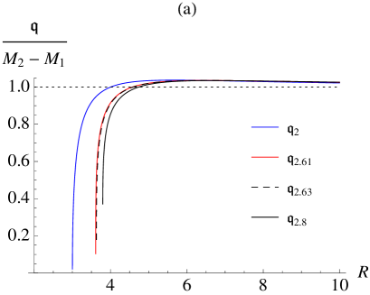
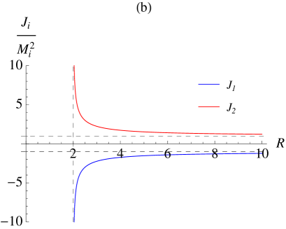
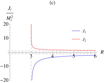
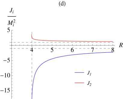
Figure 2: (a) The parameter $\mathfrak{q}$ for counter-rotating BH systems fixing $M_{1}=1$ and assigning several values in the mass $M_{2}$ labeled by the subscripts. The angular momenta $J_{1}$ and $J_{2}$ for different values of $M_{2}$, where the merging limit is indicated by a vertical line given at the distance $R=M_{1}+M_{2}$; for (b) $M_{2}=1$, (c) $M_{2}=2$, (d) $M_{2}=3$.

$M_{1}$	$M_{2}$	$R$	$\mathfrak{q}$	$J_{1}$	$J_{2}$	$J$	$\mathcal{F}$
1	1	2	0	-$\infty$	$\infty$	0	$\infty$
1	2	3.0001	0.0245	-367.439	367.531	0.0918	1667.17
1	2.618	3.6181	0.2411	-86.6621	87.7516	1.0895	44.3816
1	2.62	3.6201	0.2498	-83.7756	84.9047	1.1291	41.4199
1	3	4.0001	1.3038	-17.679	24.0594	6.3804	1.6727

Table 1: Some numerical values for extreme counter-rotating BHs. The most violent merging process occurs at the limit value $R=2m$ and it corresponds to the case of identical sources $M_{1}=M_{2}=m$, on which the interaction force $\mathcal{F}=\infty$ and each identical angular momentum $|j|=\infty$, in agreement with Ref. Herdeiro .

IV Concluding remarks

In the present paper we have worked out a concise physical representation for the two asymptotically flat $3$-parametric subfamilies of the KCH metric KCH , that may be useful to describe in a more transparent way the interactions between co/counter rotating binary BHs separated by a massless strut. In our opinion, this new parametrization is more suitable than the one presented in MR , when we want to describe the dynamical and physical properties of extreme binary systems; in particular, at the moment of choosing values on the masses and the separation distance. Additionally, our analysis has revealed that both descriptions of co/counter-rotating binary configurations are contained within the same formula for the interaction force, but their dynamical aspects differ from each other after solving a proper bicubic equation in each sector. These bicubic equations can be understood as dynamical laws for interacting BHs with struts and are special cases of that one obtained previously in Ref. Cabrera ; it reads

$$\begin{split}&\mathfrak{q}^{3}-(a_{1}+a_{2})\mathfrak{q}^{2}+(R+M)^{2}\mathfrak{q}-(R+M)[a_{1}(R+M_{1}-M_{2})+a_{2}(R-M_{1}+M_{2})]=0,\end{split}$$ (49)

being $a_{i}\equiv J_{i}/M_{i}$,   $i=1,2,$ the angular momentum per unit mass. So, once we substitute the Komar parameters $J_{i}$ of both co/counter-rotating two-body systems, their corresponding bicubic equations will emerge. Finally, we would like to pointed out that our physical representation of the KCH metric leads us to show clearly that the extreme solution saturates the Gabach Clement inequality Maria

$$\sqrt{1+4\mathcal{F}}=\frac{8\pi|J_{i}|}{S_{i}},$$ (50)

where $\mathcal{F}$ is given by Eqs. (34) and (45), while $S_{i}$ represents the area of the horizon $S$ in the extreme limit case, obtainable after establishing $\sigma_{i}=0$ in the expression (36) of Ref. Cabrera , having that

$$S_{i}=4\pi\frac{M_{i}^{2}[(R+M)^{2}+\mathfrak{q}^{2}-2a_{i}\mathfrak{q}]^{2}+a_{i}^{2}(R^{2}-\Delta)^{2}}{R^{2}[(R+M)^{2}+\mathfrak{q}^{2}]},$$ (51)

and therefore, it can be shown that the equality is reached after placing the angular momenta on each rotating sector.

References

• (1) W. Kinnersley and D. M. Chitre, J. Math. Phys. (N.Y.) 19, 2037 (1978).
• (2) D. Kramer and G. Neugebauer, Phys. Lett. A 75, 259 (1980).
• (3) M. Yamazaki, Prog. Theor. Phys. 63, 1950 (1980).
• (4) E. Newman, L. Tamburino, and T. Unti, J. Math. Phys. (N.Y.) 4, 915 (1963).
• (5) A. Tomimatsu and H. Sato, Prog. Theor. Phys. 50, 95 (1973).
• (6) V. S. Manko and E. Ruiz, Prog. Theor. Phys. 125, 1241 (2011).
• (7) R. Bach and H. Weyl, Math. Z. 13, 134 (1922).
• (8) W. Israel, Phys. Rev. D 15, 935 (1977).
• (9) A. Komar, Phys. Rev. 113, 934 (1959).
• (10) A. Papapetrou, Proc. R. Irish Acad. Sect. A 51, 191 (1947).
• (11) F. J. Ernst, Phys. Rev. 167, 1175 (1968).
• (12) R. Geroch, J. Math. Phys. 11, 2580 (1970).
• (13) R. O. Hansen, J. Math. Phys. 15, 46 (1974).
• (14) D. Fodor , C. Hoenselaers, and Z. Perjés, J. Math. Phys. 30, 2252 (1989).
• (15) N. R. Sibgatullin, Oscillations and Waves in Strong Gravitational and Electromagnetic Fields, Springer-Verlag, Berlin, 1991.
• (16) Z. Perjés, J. Math. Phys. (N.Y.) 30, 2197 (1989).
• (17) I. Cabrera-Munguia, arXiv:1806.05442v1.
• (18) A. Tomimatsu, Prog. Theor. Phys. 70, 385 (1983).
• (19) Weinstein G, Commun. Pure Appl. Math. 43, 903 (1990).
• (20) W. Dietz C. Hoenselaers, Ann. Phys. (N.Y.) 165, 319 (1985).
• (21) C. Hoenselaers, Prog. Theor. Phys. 72, 761 (1984).
• (22) R. Schoen and S.-T. Yau, Commun. Math. Phys. 65, 45 (1979).
• (23) R. Schoen and S.-T. Yau, Commun. Math. Phys. 79, 231 (1981).
• (24) Miguel S. Costa, Carlos A. R. Herdeiro, and Carmen Rebelo, Phys. Rev. D, 79, 123508 (2009).
• (25) I. Cabrera-Munguia, V. E. Ceron, L. A. López, and Omar Pedraza, Phys. Lett. B 772, 10 (2017).
• (26) G. G. Varzugin, Theor. Math. Phys. 116, 1024 (1998).
• (27) C. A. R. Herdeiro and C. Rebelo, JHEP 0810, 017 (2008).
• (28) V. S. Manko, E. D. Rodchenko, E. Ruiz, and B. I. Sadovnikov, Phys. Rev. D 78, 123508 (2008).
• (29) M. E. Gabach Clement, Class. Quantum Grav. 29, 165008 (2012).