Abstract

We use surrogate losses to obtain several new regret bounds and new algorithms for contextual bandit learning. Using the ramp loss, we derive new margin-based regret bounds in terms of standard sequential complexity measures of a benchmark class of real-valued regression functions. Using the hinge loss, we derive an efficient algorithm with a $\sqrt{dT}$-type mistake bound against benchmark policies induced by $d$-dimensional regressors. Under realizability assumptions, our results also yield classical regret bounds.

1 Introduction

We study sequential prediction problems with partial feedback, mathematically modeled as contextual bandits (Langford and Zhang, 2008). In this formalism, a learner repeatedly (a) observes a context, (b) selects an action, and (c) receives a loss for the chosen action. The objective is to learn a policy for selecting actions with low loss, formally measured via regret with respect to a class of benchmark policies. Contextual bandit algorithms have been successfully deployed in online recommendation systems (Agarwal et al., 2016), mobile health platforms (Tewari and Murphy, 2017), and elsewhere.

In this paper, we use surrogate loss functions to derive new margin-based algorithms and regret bounds for contextual bandits. Surrogate loss functions are ubiquitous in supervised learning (cf. Zhang (2004); Bartlett et al. (2006); Schapire and Freund (2012)). Computationally, they are used to replace NP-hard optimization problems with tractable ones, e.g., the hinge loss makes binary classification amenable to convex programming techniques. Statistically, they also enable sharper generalization analysis for models including boosting, SVMs, and neural networks (Schapire and Freund, 2012; Anthony and Bartlett, 2009), by replacing dependence on dimension in VC-type bounds with distribution-dependent quantities. For example, to agnostically learn $d$-dimensional halfspaces the optimal rates for excess risk are $\sqrt{d/n}$ for the $0/1$ loss benchmark and $\frac{1}{\gamma}\cdot\sqrt{1/n}$ for the $\gamma$-margin loss benchmark (Kakade et al., 2009), meaning the margin bound removes explicit dependence on dimension. Curiously, surrogate losses have seen limited use in partial information settings (some exceptions are discussed below). This paper demonstrates that these desirable computational and statistical properties indeed extend to contextual bandits.

In the first part of the paper we focus on statistical issues, namely whether any algorithm can achieve a generalization of the classical margin bound from statistical learning (Boucheron et al., 2005) in the adversarial contextual bandit setting. Our aim here is to introduce a theory of learnability for contextual bandits, in analogy with statistical and online learning, and our results provide an information-theoretic benchmark for future algorithm designers. We consider benchmark policies induced by a class of real-valued regression functions and obtain a regret bound in terms of the class’ sequential metric entropy, a standard complexity measure in online learning (Rakhlin et al., 2015b). As a consequence, we show that $\tilde{\mathcal{O}}(T^{\frac{d}{d+1}})$ regret is achievable for Lipschitz contextual bandits in $d$-dimensional metric spaces, improving on a recent result of Cesa-Bianchi et al. (2017), and that an $\tilde{O}(T^{2/3})$ mistake bound is achievable for bandit multiclass prediction in smooth Banach spaces, extending Kakade et al. (2008).

Technically, these results build on the non-constructive minimax analysis of Rakhlin et al. (2015b), which, for the online adversarial setting, prescribes a recipe for characterizing statistical behavior of arbitrary classes, and thus provides a counterpart to empirical risk minimization in statistical learning. Indeed, for full-information problems, this approach yields regret bounds in terms of sequential analogues of standard complexity measures including Rademacher complexity and metric entropy. However, since we work in the contextual bandit setting, we must extend these arguments to incorporate partial information. To do so, we leverage the adaptive minimax framework of Foster et al. (2015) along with a careful “adaptive" chaining argument.

In the second part of the paper, we focus on computational issues and derive two new algorithms using the hinge loss as a convex surrogate. The first algorithm, Hinge-LMC, provably runs in polynomial time and achieves a $\sqrt{dT}$-mistake bound against $d$-dimensional benchmark regressors with convexity properties. Hinge-LMC is the first efficient algorithm with $\sqrt{dT}$-mistake bound for bandit multiclass prediction using a surrogate loss without curvature, and so it provides a new resolution to the open problem of Abernethy and Rakhlin (2009). This algorithm is based on the exponential weights update, along with Langevin Monte Carlo for efficient sampling and a careful action selection scheme. The second algorithm is much simpler: in the stochastic setting, Follow-The-Leader with appropriate smoothing matches our information-theoretic results for sufficiently large classes.

1.1 Preliminaries

Let $\mathcal{X}$ denote a context space and $\mathcal{A}=\{1,\ldots,K\}$ a discrete action space. In the adversarial contextual bandits problem, for each of $T$ rounds, an adversary chooses a pair $(x_{t},\ell_{t})$ where $x_{t}\in\mathcal{X}$ is the context and $\ell_{t}\in[0,1]^{K}\triangleq\mathcal{L}$ is a loss vector. The learner observes the context $x_{t}$, chooses an action $a_{t}$, and incurs loss $\ell_{t}(a_{t})\in[0,1]$, which is also observed. The goal of the learner is to minimize the cumulative loss over the $T$ rounds, and, in particular, we would like to design learning algorithms that achieve low regret against a class $\Pi\subset\left(\mathcal{X}\to\mathcal{A}\right)$ of benchmark policies:

$$\textrm{Regret}(T,\Pi)\triangleq\sum_{t=1}^{T}\mathbb{E}[\ell_{t}(a_{t})]-\inf_{\pi\in\Pi}\sum_{t=1}^{T}\mathbb{E}[\ell_{t}(\pi(x_{t}))].$$

In this paper, we always identify $\Pi$ with a class of vector-valued regression functions $\mathcal{F}\subset(\mathcal{X}\to\mathbb{R}_{=0}^{K})$, where $\mathbb{R}_{=0}^{K}\triangleq\{s\in\mathbb{R}^{K}:\sum_{a}s_{a}=0\}$. We use the notation $f(x)\in\mathbb{R}^{K}$ to denote the vector-valued output and $f(x)_{a}$ to denote the $a^{\textrm{th}}$ component. Note that we are assuming $\sum_{a}f(x)_{a}=0$, which is a natural generalization of the standard formulation for binary classification (Bartlett et al., 2006) and appears in Pires et al. (2013). Define $B\triangleq\sup_{f\in\mathcal{F}}\sup_{x\in\mathcal{X}}\left\|f(x)\right\|_{\infty}$ to be the maximum value predicted by any regressor.

Our algorithms use importance weighting to form unbiased loss estimates. If at round $t$, the algorithm chooses action $a_{t}$ by sampling from a distribution $p_{t}\in\Delta(\mathcal{A})$, the loss estimate is defined as $\hat{\ell}_{t}(a)\triangleq\ell_{t}(a_{t}){\textbf{1}}\{a_{t}=a\}/p_{t}(a)$. Given $p_{t}$, we also define a smoothed distribution as $p_{t}^{\mu}\triangleq(1-K\mu)p_{t}+\mu$ for some parameter $\mu\in[0,1/K]$.

We introduce two surrogate loss functions, the ramp loss and the hinge loss, whose scalar versions are defined as $\phi^{\gamma}(s)\triangleq\min(\max(1+s/\gamma,0),1)$ and $\psi^{\gamma}(s)\triangleq\max(1+s/\gamma,0)$ respectively, for $\gamma>0$. For $s\in\mathbb{R}^{K}$, $\phi^{\gamma}(s)$ and $\psi^{\gamma}(s)$ are defined coordinate-wise. We start with a simple lemma, demonstrating how $\phi^{\gamma},\psi^{\gamma}$ act as surrogates for cost-sensitive multiclass losses.

Lemma 1 (Surrogate Loss Translation).

For $s\in\mathbb{R}_{=0}^{K}$, define $\pi_{\textrm{ramp}}(s),\pi_{\textrm{hinge}}(s)\in\Delta(\mathcal{A})$ by $\pi_{\textrm{ramp}}(s)_{a}\propto\phi^{\gamma}(s_{a})$ and $\pi_{\textrm{hinge}}(s)_{a}\propto\psi^{\gamma}(s_{a})$. For any vector $\ell\in\mathbb{R}^{K}_{+}$, we have

$$\langle\pi_{\textrm{ramp}}(s),\ell\rangle \leq\langle\ell,\phi^{\gamma}(s)\rangle\leq\sum_{a\in\mathcal{A}}\ell(a)\textup{{{1}}}\{s_{a}\geq-\gamma\},\qquad\text{and}\qquad\langle\pi_{\textrm{hinge}}(s),\ell\rangle\leq K^{-1}\langle\ell,\psi^{\gamma}(s)\rangle.$$

Based on this lemma, it will be convenient to define $L_{T}^{\gamma}(f)\triangleq\sum_{t=1}^{T}\sum_{a\in\mathcal{A}}\ell_{t}(a){\textbf{1}}\{f(x_{t})_{a}\geq-\gamma\}$, which is the margin-based cumulative loss for the regressor $f$. $L_{T}^{\gamma}$ should be seen as a cost-sensitive multiclass analogue of the classical margin loss in statistical learning (Boucheron et al., 2005). We use the term “surrogate loss” here because these quantities upper bound the cost-sensitive loss: $\ell(\mathop{\mathrm{argmax}}_{a}s_{a})\leq\langle\ell,\phi^{\gamma}(s)\rangle\leq\langle\ell,\psi^{\gamma}(s)\rangle$. In the sequel, $\pi_{\textrm{ramp}}$ and $\pi_{\textrm{hinge}}$ are used by our algorithms, but do not define the benchmark policy class, since we compare directly to $L_{T}^{\gamma}$ or the surrogate loss.

Related work.

Contextual bandit learning has been the subject of intense investigation over the past decade. The most natural categorization of these works is between parametric, realizability-based, and agnostic approaches. Parametric methods (e.g., Abbasi-Yadkori et al. (2011); Chu et al. (2011)) assume a (generalized) linear relationship between the losses and the contexts/actions. Realizability-based methods generalize parametric ones by assuming the losses are predictable by some abstract regression class (Agarwal et al., 2012; Foster et al., 2018a). Agnostic approaches (e.g., Auer et al. (2002); Langford and Zhang (2008); Agarwal et al. (2014); Rakhlin and Sridharan (2016); Syrgkanis et al. (2016a, b)) avoid realizability assumptions and instead compete with VC-type policy classes for statistical tractability. Our work contributes to all of these directions, as our margin bounds apply to the agnostic adversarial setting and yield true regret bounds under realizability assumptions.

A special case of contextual bandits is bandit multiclass prediction, where the loss vector is zero for one action and one for all others (Kakade et al., 2008). Several recent papers obtain surrogate regret bounds and efficient algorithms for this setting when the benchmark regressor class $\mathcal{F}$ consists of linear functions (Kakade et al., 2008; Hazan and Kale, 2011; Beygelzimer et al., 2017; Foster et al., 2018b). Our work contributes to this line in two ways: our bounds and algorithms extend beyond linear/parametric classes, and we consider the more general contextual bandit setting.

Our information-theoretic results on achievability are similar in spirit those of Daniely and Halbertal (2013), who derive tight generic bounds for bandit multiclass prediction in terms of the Littlestone dimension. This result is incomparable to our own: their bounds are on the $0/1$ loss regret directly rather than surrogate regret, but the Littlestone dimension is not a tight complexity measure for real-valued function classes in agnostic settings, which is our focus.

At a technical level, our work builds on several recent results. To derive achievable regret bounds, we use the adaptive minimax framework of Foster et al. (2015), along with a new adaptive chaining argument to control the supremum of a martingale process (Rakhlin et al., 2015b). Our Hinge-LMC algorithm is based on log-concave sampling (Bubeck et al., 2018), and it uses randomized smoothing (Duchi et al., 2012) and the geometric resampling trick of Neu and Bartók (2013). We also use several ideas from classification calibration (Zhang, 2004; Bartlett et al., 2006), and, in particular, the surrogate hinge loss we work with is studied by Pires et al. (2013).

2 Achievable regret bounds

This section provides generic surrogate regret bounds for contextual bandits in terms of the sequential metric entropy (Rakhlin et al., 2015a) of the regressor class $\mathcal{F}$. Notably, our general techniques apply when the ramp loss is used as a surrogate, and so, via Lemma 1, they yield the main result of the section—-a margin-based regret guarantee—as a special case.

To motivate our approach, consider a well-known reduction from bandits to full information online learning: If a full information algorithm achieves a regret bound in terms of the so-called local norms $\sum_{t}\langle p_{t},\ell_{t}^{2}\rangle$, then running the full information algorithm on importance-weighted losses $\hat{\ell}_{t}(a)$ yields an expected regret bound for the bandit setting. For example, when $\Pi$ is finite, Exp4 (Auer et al., 2002) uses Hedge (Freund and Schapire, 1997) as the full information algorithm, and obtains a deterministic regret bound of

$$\textrm{Regret}(T,\Pi)\leq\frac{\eta}{2}\sum_{t=1}^{T}\operatorname{\mathbb{E}}_{\pi\sim{}p_{t}}\left\langle\pi(x_{t}),\hat{\ell}_{t}\right\rangle^{2}+\frac{\log(|\Pi|)}{\eta},$$ (1)

where $\eta>0$ is the learning rate and $p_{t}$ is the distribution over policies in $\Pi$ (inducing an action distribution) for round $t$. Evaluating conditional expectations and optimizing $\eta$ yields a regret bound of $\mathcal{O}(\sqrt{KT\log(|\Pi|)})$, which is optimal for contextual bandits with a finite policy class.

To use this reduction beyond the finite class case and with surrogate losses we face two challenges:

1. Infinite classes. The natural approach of using a pointwise (or sup-norm) cover for $\mathcal{F}$ is insufficient—not only because there are classes that have infinite pointwise covers yet are online-learnable, but also because it yields sub-optimal rates even when a finite pointwise cover is available. Instead, we establish existence of a full-information algorithm for large nonparametric classes that has 1) strong adaptivity to loss scaling as in (1) and 2) regret scaling with the sequential covering number for $\mathcal{F}$, which is the correct generalization of the empirical covering number in statistical learning to the adversarial online setting. This is achieved via non-constructive methods.

2. Variance control. With surrogate losses, controlling the variance/local norm term $\mathbb{E}_{\pi}\langle\pi(x_{t}),\hat{\ell}_{t}\rangle^{2}$ in the reduction from bandit to full information is more challenging, since the surrogate loss of a policy depends on the scale of the underlying regressor, not just the action it selects. To address this, we develop a new sampling scheme tailored to scale-sensitive losses.

Full-information regret bound.

We consider the following full information protocol, which in the sequel will be instantiated via reduction from contextual bandits. Let the context space $\mathcal{X}$ and $\mathcal{A}$ be fixed as in Subsection 1.1, and consider a function class $\mathcal{G}\subset(\mathcal{X}\to\mathcal{S})$, where $\mathcal{S}\subseteq{}\mathbb{R}^{K}_{+}$. The reader may think of $\mathcal{G}$ as representing $\phi^{\gamma}\circ\mathcal{F}$ or $\psi^{\gamma}\circ\mathcal{F}$, i.e. the surrogate loss composed with the regressor class, so that $\mathcal{S}$ (which is not necessarily convex) represents the image of the surrogate loss over $\mathcal{F}$.

The online learning protocol is: For time $t=1,\ldots,T$, (1) the learner observes $x_{t}$ and chooses a distribution $p_{t}\in\Delta(\mathcal{S})$, (2) the adversary picks a loss vector $\ell_{t}\in{}\mathcal{L}\subset{}\mathbb{R}^{K}_{+}$, (3) the learner samples outcome $s_{t}\sim{}p_{t}$ and experiences loss $\left\langle s_{t},\ell_{t}\right\rangle$. Regret against the benchmark class $\mathcal{G}$ is given by

$$\sum_{t=1}^{T}\operatorname{\mathbb{E}}_{s_{t}\sim{}p_{t}}\left\langle s_{t},\ell_{t}\right\rangle-\inf_{g\in\mathcal{G}}\sum_{t=1}^{T}\left\langle g(x_{t}),\ell_{t}\right\rangle.$$

As our complexity measure, we use a multi-output generalization of sequential covering numbers introduced by Rakhlin et al. (2015a). Define a $\mathcal{Z}$-valued tree $\bm{z}$ to be a sequence of mappings $\bm{z}_{t}:\left\{\pm{}1\right\}^{t-1}\to\mathcal{Z}$. The tree $\bm{z}$ is a complete rooted binary tree with nodes labeled by elements of $\mathcal{Z}$, where for any “path” $\epsilon\in\left\{\pm{}1\right\}^{T}$, $\bm{z}_{t}(\epsilon)\triangleq\bm{z}_{t}(\epsilon_{1:t-1})$ is the value of the node at level $t$ on the path $\epsilon$.

Definition 1.

For a function class $\mathcal{G}\subset(\mathcal{X}\to\mathbb{R}^{K})$ and $\mathcal{X}$-valued tree $\bm{x}$ of length $T$, the $L_{\infty}/\ell_{\infty}$ sequential covering number for $\mathcal{G}$ on $\bm{x}$ at scale $\varepsilon$, denoted by $\mathcal{N}_{\infty,\infty}(\varepsilon,\mathcal{G},\bm{x})$, is the cardinality of the smallest set $V$ of $\mathbb{R}^{K}$-valued trees for which

$$\forall{}g\in\mathcal{G}\;\forall{}\epsilon\in\left\{\pm{}1\right\}^{T}\;\exists{}\bm{v}\in{}V\textnormal{ s.t. }\max_{t\in\left[T\right]}\left\|g(\bm{x}_{t}(\epsilon))-\bm{v}_{t}(\epsilon)\right\|_{\infty}\leq\varepsilon.$$ (2)

Define $\mathcal{N}_{\infty,\infty}(\varepsilon,\mathcal{G},T)\triangleq\sup_{\bm{x}:\mathrm{length}(\bm{x})=T}\mathcal{N}_{\infty,\infty}(\varepsilon,\mathcal{G},\bm{x})$.

We refer to $\log\mathcal{N}_{\infty,\infty}$ as the sequential metric entropy. Note that in the binary case, for learning unit $\ell_{2}$ norm linear functions in $d$ dimensions, the pointwise metric entropy is $O(d\log(1/\varepsilon))$, whereas the sequential metric entropy is $O(d\log(1/\varepsilon)\wedge\varepsilon^{-2}\log(d))$, leading to improved rates in high dimension.

With this definition, we can now state our main theorem for full information.

Theorem 2.

Assume $\sup_{\ell\in\mathcal{L}}\left\|\ell\right\|_{1}\leq{}R$ and $\sup_{s\in\mathcal{S}}\left\|s\right\|_{\infty}\leq{}B$. Fix any constants $\eta\in(0,1]$, $\lambda>0$, and $\beta>\alpha>0$. Then there exists an algorithm with the following deterministic regret guarantee:

$$\sum_{t=1}^{T}\operatorname{\mathbb{E}}_{s_{t}\sim{}p_{t}}\left\langle s,\ell_{t}\right\rangle-\inf_{g\in\mathcal{G}}\sum_{t=1}^{T}\left\langle g(x_{t}),\ell_{t}\right\rangle \leq{}\frac{2\eta}{RB}\sum_{t=1}^{T}\operatorname{\mathbb{E}}_{s_{t}\sim{}p_{t}}\left\langle s_{t},\ell_{t}\right\rangle^{2}+\frac{4RB}{\eta}\log\mathcal{N}_{\infty,\infty}(\beta/2,\mathcal{G},T)+3e^{2}\alpha\sum_{t=1}^{T}\left\|\ell_{t}\right\|_{1}$$

$$~{}~{}~{}~{}~{}+24e\left(\frac{\lambda}{4R}\sum_{t=1}^{T}\left\|\ell_{t}\right\|_{1}^{2}+\frac{R}{\lambda}\right)\int_{\alpha}^{\beta}\sqrt{\log\mathcal{N}_{\infty,\infty}(\varepsilon,\mathcal{G},T)}d\varepsilon.$$

Observe that the bound involves the variance/local norms $\operatorname{\mathbb{E}}_{s_{t}\sim{}p_{t}}\left\langle s_{t},\ell_{t}\right\rangle^{2}$, and has a very mild explicit dependence on the loss range $R$; this can be verified by optimizing over $\eta$ and $\lambda$. This adaptivity to the loss range is crucial for our bandit reduction. Further observe that the bound contains a Dudley-type entropy integral, which is essential for obtaining sharp rates for complex nonparametric classes.

Bandit reduction and variance control.

To lift Theorem 2 to contextual bandits we use the following reduction: First, initialize the full information algorithm from Theorem 2 with $\mathcal{G}=\phi^{\gamma}\circ\mathcal{F}$. For each round $t$, receive $x_{t}$, and define $P_{t}(a)\triangleq\operatorname{\mathbb{E}}_{s_{t}\sim{}p_{t}}\frac{s_{t}(a)}{\sum_{a^{\prime}\in\left[K\right]}s_{t}(a^{\prime})}$ where $p_{t}$ is the full information algorithm’s distribution. Then sample $a_{t}\sim P_{t}^{\mu}$, observe $\ell_{t}(a_{t})$, and pass the importance-weighted loss $\hat{\ell}_{t}(a)$ back to the algorithm. For the hinge loss we use the same strategy, but with $\mathcal{G}=\psi^{\gamma}\circ\mathcal{F}$.

The following lemma shows that this strategy leads to sufficiently small variance in the loss estimates. The definition of the action distribution $P^{\mu}_{t}(a)$ in terms of the real-valued predictions is crucial here.

Lemma 3.

Define a filtration $\mathcal{J}_{t}=\sigma((x_{1},\ell_{1},a_{1}),\ldots,(x_{t-1},\ell_{t-1},a_{t-1}),x_{t},\ell_{t})$. Then for any $\mu\in[0,1/K]$ the importance weighting strategy above guarantees

$$\operatorname{\mathbb{E}}_{a_{t}\sim P_{t}^{\mu}}\left[\operatorname{\mathbb{E}}_{s_{t}\sim{}p_{t}}\left\langle s_{t},\hat{\ell}_{t}\right\rangle^{2}\mid{}\mathcal{J}_{t}\right]\leq{}\left\{\begin{array}[]{ll}K,&\quad\text{ for ${\mathcal{S}}\subset\Delta(\mathcal{A})$.}\\ K^{2},&\quad\text{ for ${\mathcal{S}}=\phi^{\gamma}\circ\mathcal{F}$.}\\ \left(1+\frac{B}{\gamma}\right)^{2}K^{2},&\quad\text{ for ${\mathcal{S}}=\psi^{\gamma}\circ\mathcal{F}$.}\end{array}\right.$$

Theorem 2 and Lemma 3 together imply our central theorem: a chaining-based margin bound for contextual bandits, generalizing classical results in statistical learning (cf. (Boucheron et al., 2005)).

Theorem 4 (Contextual bandit margin bound).

For any fixed constants $\beta>\alpha>0$, smoothing parameter $\mu\in(0,1)$ and margin loss parameter $\gamma>0$ there exists an adversarial contextual bandit strategy with expected regret against the $\gamma$-margin benchmark bounded as

$$\operatorname{\mathbb{E}}\left[\sum_{t=1}^{T}\ell_{t}(a_{t})\right]\leq{} \inf_{f\in\mathcal{F}}\operatorname{\mathbb{E}}\left[L_{T}^{\gamma}(f)\right]+4\sqrt{2K^{2}T\log\mathcal{N}_{\infty,\infty}(\beta/2,\mathcal{F},T)}+\mu{}KT$$ (3)

$$~{}~{}~{}~{}~{}~{}~{}+\frac{8}{\mu}\log\mathcal{N}_{\infty,\infty}(\beta/2,\mathcal{F},T)+\frac{1}{\gamma}\left(3e^{2}\alpha{}KT+24e\sqrt{\frac{KT}{\mu}}\int_{\alpha}^{\beta}\sqrt{\log\mathcal{N}_{\infty,\infty}(\varepsilon,\mathcal{F},T)}d\varepsilon\right).$$

We derive an analogous bound for the hinge loss in Appendix C. The hinge loss bound differs only through stronger dependence on scale parameters.

Before showing the implications of Theorem 4 for specific classes $\mathcal{F}$ we state a coarse upper bound in terms of the growth rate for the sequential metric entropy.

Proposition 5.

Suppose that $\mathcal{F}$ has sequential metric entropy growth $\log\mathcal{N}_{\infty,\infty}(\varepsilon,\mathcal{F},T)\propto\varepsilon^{-p}$ for some $p>0$ (nonparametric case), or that $\log\mathcal{N}_{\infty,\infty}(\varepsilon,\mathcal{F},T)\propto{}d\log(1/\varepsilon)$ (parametric case). Then there exists a contextual bandit strategy with the following regret guarantee:

$$\operatorname{\mathbb{E}}\left[\sum_{t=1}^{T}\ell_{t}(a_{t})\right]\leq{}\inf_{f\in\mathcal{F}}\operatorname{\mathbb{E}}\left[L_{T}^{\gamma}(f)\right]+\left\{\begin{array}[]{ll}O(K\sqrt{dT\log(KT/\gamma)}),&~{}~{}\text{parametric case.}\\ \tilde{O}((KT)^{\frac{p+2}{p+4}}\gamma^{-\frac{2p}{p+4}}),&~{}~{}\text{nonparametric w/~{}~{}}p\leq{}2.\\ \tilde{O}((KT)^{\frac{p}{p+1}}\gamma^{-\frac{p}{p+1}}),&~{}~{}\text{nonparametric w/~{}~{}}p\geq{}2.\end{array}\right.$$ (4)

Proposition 5 recovers the parametric rate of $\sqrt{dT}$ seen with e.g., LinUCB (Chu et al., 2011) but is most interesting for complex classes. The rate exhibits a phase change between the “moderate complexity” regime of $p\in(0,2]$ and the “high complexity” regime of $p\geq{}2$. This is visualized in Figure 1.

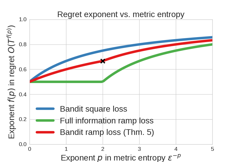
Figure 1: Regret bound exponent as a function of (sequential) metric entropy. The cross marks the point $p=2$ where the exponent from Theorem 4 changes growth rate. “Full information” refers to the optimal rate of $T^{\frac{1}{2}\vee{}(\frac{p-1}{p})}$ for the same setting under full information feedback (Rakhlin et al., 2015a). “Square loss” refers to the optimal rate of $T^{\frac{p+1}{p+2}}$ for Lipschitz contextual bandits over metric spaces of dimension $p$, which have sequential metric entropy $\varepsilon^{-p}$, under square loss realizability (Slivkins, 2011).

Remark 1.

Under i.i.d. losses and hinge/ramp loss realizability, the standard tools of classification calibration (Bartlett et al., 2006) can be used to deduce a proper policy regret bound from (3). However, these realizability assumptions are somewhat non-standard, and moreover if one imposes the stronger assumption of a hard margin it is possible to derive improved rates (Daniely and Halbertal, 2013). See also Appendix B.

Remark 2.

Classical margin bounds typically hold for all values of $\gamma$ simultaneously, but Theorem 4 requires that $\gamma$ is chosen in advance. Learning the best value of $\gamma$ online appears challenging.

Rates for specific classes.     We now instantiate our results for concrete classes of interest.

Example 1 (Finite classes).

In the finite class case there is an algorithm with $O\left(K\sqrt{T\log\left\lvert\mathcal{F}\right\rvert}\right)$ margin regret. When $\Pi\subset(\mathcal{X}\to\mathcal{A})$ is a finite policy class, directly reducing to Theorem 2 yields the optimal $O\left(\sqrt{KT\log\left\lvert\Pi\right\rvert}\right)$ policy regret, hinting at the optimality of our approach.

Example 2 (Lipschitz CB).

The class of Lipschitz functions over $\left[0,1\right]^{p}$ admits a sequential cover with metric entropy $\tilde{O}(\varepsilon^{-p})$, so Proposition 5 implies an $\tilde{\mathcal{O}}(T^{\frac{p+2}{p+4}\vee\frac{p}{p+1}})$ regret bound. Since our proof goes through Lemma 1, it also yields a policy regret bound against the $\pi_{\textrm{ramp}}(\cdot)$ class. Therefore, this result is directly comparable to the $\tilde{\mathcal{O}}(T^{\frac{p+1}{p+2}})$ bound of Cesa-Bianchi et al. (2017), applied to the $\pi_{\textrm{ramp}}$ policy class. Our bound achieves a smaller exponent for all values of $p$ (see Figure 1).

Learnability in full information online learning is known to be characterized entirely by the sequential Rademacher complexity of the hypothesis class (Rakhlin et al., 2015a), and tight bounds on this quantity are known for standard classes including linear predictors, decision trees, and neural networks. The next example, a corollary of Theorem 4, bounds contextual bandit margin regret in terms of sequential Rademacher complexity, which is defined for any scalar-valued function class $\mathcal{G}\subseteq{}\left(\mathcal{X}\to\mathbb{R}\right)$ as:

$$\mathfrak{R}(\mathcal{G},T)\triangleq\sup_{\bm{x}}\operatorname{\mathbb{E}}_{\epsilon}\sup_{g\in\mathcal{G}}\sum_{t=1}^{T}\epsilon_{t}g(\bm{x}_{t}(\epsilon)).$$

Example 3.

Let $\mathcal{F}|_{a}\triangleq\left\{x\mapsto{}f(x)_{a}\mid{}f\in\mathcal{F}\right\}$ be the scalar restriction of $\mathcal{F}$ to output coordinate $a$ and suppose that $\max_{a\in\left[K\right]}\mathfrak{R}(\mathcal{F}|_{a},T)\geq{}1$ and $B\leq{}1$. Then there exists an adversarial contextual bandit algorithm with margin regret bound $\tilde{O}\left(\max_{a}K\left(\mathfrak{R}(\mathcal{F}|_{a},T)/\gamma\right)^{2/3}T^{1/3}\right)$.

Thus, for margin-based contextual bandits, full information learnability is equivalent to bandit learnability. Since the optimal regret in full information is $\Omega(\max_{a}\mathfrak{R}(\mathcal{F}|_{a},T))$, it further shows that the price of bandit information is at most $\tilde{O}\left(\max_{a}K\left(T/\mathfrak{R}(\mathcal{F}|_{a},T)\right)^{1/3}\right)$. Note that while this bound is fairly user-friendly, it yields worse rates than Proposition 5 when translated to sequential metric entropy, except when $p=2$ (Rakhlin et al., 2010). For comparison, Rakhlin et al. (2015a) obtain $\tilde{O}(\mathfrak{R}(\mathcal{F},T)/\gamma)$ margin regret in full information for binary classification. For partial information, BISTRO (Rakhlin and Sridharan, 2016) has an $O(\sqrt{KT\mathfrak{R}(\Pi,T)})$ policy regret bound, which involves the policy complexity and a worse $T$ dependence than our bound, but our bound (in terms of $\mathcal{F}$) applies only to the margin regret. A similar discussion applies to Theorem 4.4 of Lykouris et al. (2018).

Instantiating Example 3 with linear classes generalizes the $O(T^{2/3})$ dimension-independent guarantee of Banditron (Kakade et al., 2008) from Euclidean geometry to arbitrary uniformly convex Banach spaces, essentially the largest linear class for which online learning is possible (Srebro et al., 2011). The result also generalizes Banditron from multiclass to general contextual bandits and strengthens it from hinge loss to ramp loss. Note that many subsequent works (Abernethy and Rakhlin, 2009; Beygelzimer et al., 2017; Foster et al., 2018b) obtain dimension-dependent $O(\sqrt{dT})$ bounds for bandit multiclass prediction, as we will in the next section, but, none have explored dimension-independent $O(T^{2/3})$-type rates, which are more appropriate for high-dimensional settings.

Example 4.

Let $\mathcal{X}$ be the unit ball in a Banach space $(\mathfrak{B},\left\|\cdot\right\|)$, and let $\mathcal{F}$ be induced by stacking $K-1$ linear predictors each in the unit ball of the dual space $(\mathfrak{B}^{\star},\left\|\cdot\right\|_{\star})$. Suppose that $\left\|\cdot\right\|$ has martingale type 2 (Pisier, 1975), which means there exists $\Psi:\mathfrak{B}\to\mathbb{R}$ such that $\frac{1}{2}\left\|x\right\|^{2}\leq{}\Psi(x)$ and $\Psi$ is $\beta$-smooth w.r.t. $\left\|\cdot\right\|$. Then there exists a contextual bandit strategy with margin regret $O(K(T/\gamma)^{2/3})$.

Beyond linear classes, we also obtain $\tilde{O}(K(T/\gamma)^{2/3})$ margin regret when each $\mathcal{F}_{a}$ is a class of neural networks with weights in each layer bounded in the $(1,\infty)$ group norm, or when each $\mathcal{F}_{a}$ is a class of bounded depth decision trees on finitely many decision functions. These results follow by appealing to the existing sequential Rademacher complexity bounds derived in Rakhlin et al. (2015a).

As our last example, we consider $\ell_{p}$ spaces for $p<2$. These spaces fail to satisfy martingale type 2 in a dimension-independent fashion, but they do satisfy martingale type $p$ without dimension dependence, and so have sequential metric entropy of order $\varepsilon^{-\frac{p}{p-1}}$ (Rakhlin and Sridharan, 2017). Moreover, in $\mathbb{R}^{d}$ the $\ell_{p}$ spaces admit a pointwise cover with metric entropy $O(d\log(1/\varepsilon))$, leading to the following dichotomy.

Example 5.

Consider the setting of Example 4, with $(\mathfrak{B},\left\|\cdot\right\|)=(\mathbb{R}^{d},\left\|\cdot\right\|_{p})$ for $p\leq{}2$. Then there exists a contextual bandit strategy with margin regret $\tilde{O}(K(T/\gamma)^{\frac{p}{2p-1}}\wedge{}K\sqrt{dT\log(KT/\gamma)})$.

3 Efficient algorithms

We derive two new algorithms for contextual bandits using the hinge loss $\psi^{\gamma}$. The first algorithm, Hinge-LMC, focuses on the parametric setting; it is based on a continuous version of exponential weights using a log-concave sampler. The second, SmoothFTL, is simply Follow-The-Leader with uniform smoothing. SmoothFTL applies to the stochastic setting with classes that have “high complexity” in the sense of Proposition 5.

3.1 Hinge-LMC

For this section, we identify $\mathcal{F}$ with a compact convex set $\Theta\subset\mathbb{R}^{d}$, using the notation $f(x;\theta)\in\mathbb{R}_{=0}^{K}$ to describe the parametrized function. We assume that $\psi^{\gamma}(f(x;\theta)_{a})$ is convex in $\theta$ for each $(x,a)$ pair, $\sup_{x,\theta}\|f(x;\theta)\|_{\infty}\leq B$, $f(x;\cdot)_{a}$ is $L$-Lipschitz in $\theta$ with respect to the $\ell_{2}$ norm, and that $\Theta$ contains the centered Euclidean ball of radius $1$ and is contained within a Euclidean ball of radius $R$. These assumptions are satisfied when $\mathcal{F}$ is a linear class, under appropriate boundedness conditions.

Input: Class $\Theta$, learning rate $\eta$, margin parameter $\gamma$.

Define $w_{0}(\theta)\triangleq 1$ for all $\theta\in\Theta$.

for $t=1,\ldots,T$ do

     Receive $x_{t}$, set $\theta_{t}\leftarrow$ LMC($\eta w_{t-1}$).

     Set $p_{t}(\cdot;\theta_{t})\propto\psi^{\gamma}(f(x_{t};\theta_{t}))$.

     Set $p^{\mu}_{t}(\cdot;\theta_{t})\triangleq(1-K\mu)p_{t}+\mu$.

     Play $a_{t}\sim p_{t}^{\mu}(\cdot;\theta_{t})$, observe $\ell_{t}(a_{t})$.

     // Geometric resampling.

     for $m=1,\ldots,M$ do

         $\tilde{\theta}_{t}\leftarrow$ LMC($\eta w_{t-1}$).

         Sample $\tilde{a}_{t}\sim p^{\mu}_{t}(\cdot;\tilde{\theta}_{t})$, if $\tilde{a}_{t}=a_{t}$, break.

     end for

     Set $m_{t}=m$, and $\tilde{\ell}_{t}(a)\triangleq\ell_{t}(a_{t})\cdot{}m_{t}{\textbf{1}}\{a_{t}=a\}$.

     Update $w_{t}(\theta)\leftarrow w_{t-1}(\theta)+\langle\tilde{\ell}_{t},\psi^{\gamma}(f(x_{t};\theta))\rangle$.

end for

Algorithm 1 Hinge-LMC

Input: $F(\cdot)$, parameters $m,u,\lambda,N,\alpha$.

// Parameter choices are in Appendix D.

Set $\tilde{\theta}_{0}\leftarrow 0\in\mathbb{R}^{d}$

for $k=1,\ldots,N$ do

     Draw $z_{1},\ldots,z_{m}\stackrel{{\scriptstyle{iid}}}{{\sim}}\mathcal{N}(0,u^{2}I_{d})$. Define

$$\tilde{F}_{k}(\theta)\triangleq\tfrac{1}{m}\textstyle\sum\nolimits_{i=1}^{m}F(\theta+z_{i})+\frac{\lambda}{2}\|\theta\|_{2}^{2}$$

     Draw $\xi_{k}\sim\mathcal{N}(0,I_{d})$ and update

$$\tilde{\theta}_{k}\leftarrow\mathcal{P}_{\Theta}\left(\tilde{\theta}_{k-1}-\frac{\alpha}{2}\nabla\tilde{F}_{k}(\tilde{\theta}_{k-1})+\sqrt{\alpha}\xi_{k}\right).$$

end for

Return $\tilde{\theta}_{N}$.

Algorithm 2 Langevin Monte Carlo (LMC)

The pseudocode for Hinge-LMC is displayed in Algorithm 1, and all parameters settings are given in Appendix D. The algorithm is a continuous variant of exponential weights (Auer et al., 2002), where at round $t$, we define the exponential weights distribution via its density (w.r.t. the Lebesgue measure over $\Theta$):

$$P_{t}(\theta)\propto\exp(-\eta w_{t-1}(\theta)),\qquad w_{t-1}(\theta)\triangleq\sum_{s=1}^{t-1}\langle\tilde{\ell}_{s},\psi^{\gamma}(f(x_{s};\theta))\rangle,$$

where $\eta$ is a learning rate and $\tilde{\ell}_{s}$ is a loss vector estimate. At a high level, at each iteration the algorithm samples $\theta_{t}\sim P_{t}$, then samples the action $a_{t}$ from the induced policy distribution $p_{t}(\cdot;\theta)=\pi_{\textrm{hinge}}(f(x_{t};\theta_{t}))$, appropriately smoothed. The algorithm plays $a_{t}$ and constructs a loss estimate $\tilde{\ell}_{t}\triangleq m_{t}\cdot\ell_{t}(a){\textbf{1}}\{a=a_{t}\}$, where $m_{t}$ is an approximate importance weight computed by repeatedly sampling from $P_{t}$. This vector $\tilde{\ell}_{t}$ is passed to exponential weights to define the distribution at the next round. To sample from $P_{t}$ we use Projected Langevin Monte Carlo (LMC), displayed in Algorithm 2.

The algorithm has many important subtleties. Apart from passing to the hinge surrogate loss to obtain a tractable log-concave sampling problem, by using the induced policy distribution $\pi_{\textrm{hinge}}(\cdot)$, we are also able to control the local norm term in the exponential weights regret bound. Then, the analysis for Projected LMC Bubeck et al. (2018) requires a smooth potential function, which we obtain by convolving with the gaussian density, also known as randomized smoothing (Duchi et al., 2012). We also use $\ell_{2}$ regularization for strong convexity and to overcome sampling errors introduced by randomized smoothing. Finally, we use the geometric resampling technique (Neu and Bartók, 2013) to approximate the importance weight by repeated sampling.

Here, we state the main guarantee and its consequences. A more complete theorem statement, with exact parameter specifications and the precise running time is provided in Appendix D as Theorem 18.

Theorem 6 (Informal).

Under the assumptions of Subsection 3.1, Hinge-LMC with appropriate parameter settings runs in time $\textrm{poly}(T,d,B,K,\tfrac{1}{\gamma},R,L)$ and guarantees

$$\mathbb{E}\sum_{t=1}^{T}\ell_{t}(a_{t})\leq\inf_{\theta\in\Theta}\frac{1}{K}\mathbb{E}\sum_{t=1}^{T}\langle\ell_{t},\psi^{\gamma}(f(x_{t};\theta))\rangle+\tilde{\mathcal{O}}\left(\frac{B}{\gamma}\sqrt{dT}\right).$$

Since bandit multiclass prediction is a special case of contextual bandits, Theorem 6 immediately implies a $\sqrt{dT}$-mistake bound for this setting. See Appendix B for more discussion.

Corollary 7 (Bandit multiclass).

In the bandit multiclass setting, Algorithm 1 enjoys a mistake bound of $\tilde{\mathcal{O}}((B/\gamma)\sqrt{dT})$ against the cost-sensitive $\gamma$-hinge loss and runs in polynomial time.

Additionally, under a realizability condition for the hinge loss, we obtain a standard regret bound. For simplicity in defining the condition, assume that for every $(x,\ell)$ pair, $\ell$ is a random variable with conditional mean $\bar{\ell}$ (chosen by the adversary) and $\bar{\ell}$ has a unique action with minimal loss.

Corollary 8 (Realizable bound).

In addition to the conditions above, assume that there exists $\theta^{\star}\in\Theta$ such that for every $(x,\ell)$ pair and for all $a\in\mathcal{A}$, we have $f(x;\theta^{\star})_{a}\triangleq K\gamma{\textbf{1}}\{\bar{\ell}(a)\leq\min_{a^{\prime}}\bar{\ell}(a^{\prime})\}-\gamma$. Then Hinge-LMC runs in polynomial time and guarantees

$$\sum_{t=1}^{T}\mathbb{E}\bar{\ell}_{t}(a_{t})\leq\sum_{t=1}^{T}\mathbb{E}\min_{a}\bar{\ell}(a)+\tilde{\mathcal{O}}\left(\frac{B}{\gamma}\sqrt{dT}\right).$$

A few comments are in order:

1. The use of LMC for sampling is not strictly necessary. Other log-concave samplers do exist for non-smooth potentials (Lovász and Vempala, 2007), which will remove the parameters $m,u,\lambda$, significantly simplify the algorithm, and even lead to a better run-time guarantee using current theory. However, we prefer to use LMC due to its success in Bayesian inference and deep learning, and its connections to incremental optimization methods. Note that more recent results in slightly different settings (Raginsky et al., 2017; Dalalyan and Karagulyan, 2017; Cheng et al., 2018) suggest that it may be possible to substantially improve upon the LMC analysis that we use and even extend it to non-convex settings. We are hopeful that the LMC approach will lead to a practically useful contextual bandit algorithm and plan to explore this direction further.

2. Corollary 7 provides a new solution to the open problem of Abernethy and Rakhlin (2009). In fact, it is the first efficient $\sqrt{dT}$-type regret bound against a hinge loss benchmark, although our loss is slightly different from the multiclass hinge loss used by Kakade et al. (2008) in their $T^{2/3}$-regret Banditron algorithm (which motivated the open problem). All prior $\sqrt{dT}$-regret algorithms (Hazan and Kale, 2011; Beygelzimer et al., 2017; Foster et al., 2018b) use losses with curvature such as the multiclass logistic loss or the squared hinge loss. See Appendix B for a comparison between cost-sensitive and multiclass hinge losses.

3. In Corollary 8, regret is measured relative to the policy that chooses the best action (in expectation) on every round. As in prior results (Abbasi-Yadkori et al., 2011; Agarwal et al., 2012), this is possible because the realizability condition ensures that this policy is in our class. Note that here, a requirement for realizability is that $B\geq K\gamma$, and hence the dependence on $K$ is implicit and in fact slightly worse than the optimal rate (Chu et al., 2011).

4. For Corollary 8, the best points of comparisons are methods based on square-loss realizability (Agarwal et al., 2012; Foster et al., 2018a), although our condition is different. Compared with LinUCB and variants (Chu et al., 2011; Abbasi-Yadkori et al., 2011) specialized to $\ell_{2}/\ell_{2}$ geometry, our assumptions are somewhat weaker but these methods have slightly better guarantees for linear classes. Compared with Foster et al. (2018a), which is the only other efficient approach at a comparable level of generality, our assumptions on the regressor class are stronger, but we obtain better guarantees, in particular removing distribution-dependent parameters.

To summarize, Hinge-LMC is the first efficient $\sqrt{dT}$-regret algorithm for bandit multiclass prediction using the hinge loss. It also represents a new approach to adversarial contextual bandits, yielding $\sqrt{dT}$ policy regret under hinge-based realizability. Finally, while we lose the theoretical guarantees, the algorithm easily extends to non-convex classes, which we expect to be practically effective.

3.2 SmoothFTL

A drawback of Hinge-LMC is that it only applies in the parametric regime. We now introduce an efficient (in terms of queries to a hinge loss minimization oracle) algorithm with a regret bound similar to Theorem 4, but in the stochastic setting, where $\left\{(x_{t},\ell_{t})\right\}_{t=1}^{T}$ are drawn i.i.d. from some joint distribution $\mathcal{D}$ over $\mathcal{X}\times{}\mathbb{R}_{+}^{K}$. Here we return to the abstract setting with regression class $\mathcal{F}$, and for simplicity, we assume $B=1$.

The algorithm we analyze is simply Follow-The-Leader with uniform smoothing and epoching, which we refer to as SmoothFTL. We use an epoch schedule where the $m^{\textrm{th}}$ epoch lasts for $n_{m}\triangleq 2^{m}$ rounds (starting with $m=0$). At the beginning of the $m^{\textrm{th}}$ epoch, we compute the empirical importance weighted hinge-loss minimizer $\hat{f}_{m-1}$ using only the data from the previous epoch. That is, we set

$$\hat{f}_{m-1}\triangleq\mathop{\mathrm{argmin}}_{f\in\mathcal{F}}\sum_{\tau=n_{m-1}}^{n_{m}-1}\langle\hat{\ell}_{\tau},\psi^{\gamma}(f(x_{\tau}))\rangle.$$

Then, for each round $t$ in the $m^{\textrm{th}}$ epoch, we sample $a_{t}$ from $p_{t}\triangleq(1-K\mu)\pi_{\textrm{hinge}}(\hat{f}_{m-1}(x_{t}))+\mu$. The parameter $\mu\in(0,1/K]$ controls the smoothing. At time $t=1$ we simply take $p_{1}$ to be uniform.

Theorem 9.

Suppose that $\mathcal{F}$ satisfies $\log\mathcal{N}_{\infty,\infty}(\varepsilon,\mathcal{F},T)\propto\varepsilon^{-p}$ for some $p>2$. Then in the stochastic setting, with $\mu=K^{-1}T^{\frac{-1}{p+1}}$, SmoothFTL enjoys the following expected regret guarantee

$$\sum_{t=1}^{T}\mathbb{E}\ell_{t}(a_{t})\leq\inf_{f\in\mathcal{F}}\frac{T}{K}\mathbb{E}\langle\ell,\psi^{\gamma}(f(x))\rangle+\tilde{O}\left((T/\gamma)^{\frac{p}{p+1}}\right).$$

This provides an algorithmic counterpart to Proposition 5 in the $p\geq 2$ regime. The algorithm is quite similar to Epoch-Greedy (Langford and Zhang, 2008), and the main contribution here is to provide a careful analysis for large function classes. We leave obtaining an oracle-efficient algorithm that matches Proposition 5 in the regime $p\in(0,2)$ as an open problem.

A similar bound can be obtained for the ramp loss by simply replacing the hinge loss ERM. We analyze the hinge loss version because standard (e.g. linear) classes admit efficient hinge loss minimization oracles. Interestingly, the bound in Theorem 9 actually improves on Proposition 5, in that it is independent of $K$. This is due to the scaling of the hinge loss in Lemma 1.

In Appendix F, we extend the analysis to the stochastic Lipschitz contextual bandit setting. Here, instead of measuring regret against the benchmark $\psi^{\gamma}\circ\mathcal{F}$ we compare to the class of all $1$-Lipschitz functions from $\mathcal{X}$ to $\Delta(\mathcal{A}$), where $\mathcal{X}$ is a metric space of bounded covering dimension. We show that SmoothFTL achieves $T^{\frac{p}{p+1}}$ regret with a $p$-dimensional context space and finite action space. This improves on the $T^{\frac{p+1}{p+2}}$ bound of Cesa-Bianchi et al. (2017), as in Example 2, yet the best available lower bound is $T^{\frac{p-1}{p}}$ (Hazan and Megiddo, 2007). Closing this gap remains an intriguing open problem.

4 Discussion

This paper initiates a study of the utility of surrogate losses in contextual bandit learning. We obtain new margin-based regret bounds in terms of sequential complexity notions on the benchmark class, improving on the best known rates for Lipschitz contextual bandits and providing dimension-independent bounds for linear classes. On the algorithmic side, we provide the first solution to the open problem of Abernethy and Rakhlin (2009) with a non-curved loss and we also show that Follow-the-Leader with uniform smoothing performs well in nonparametric settings.

Yet, several open problems remain. First, our bounds in Section 2 are likely suboptimal in the dependence on $K$, and improving this is a natural direction. Other questions involve deriving stronger lower bounds (e.g., for the non-parametric setting) and adapting to the margin parameter. We also hope to experiment with Hinge-LMC, and develop a better understanding of computational-statistical tradeoffs with surrogate losses. We look forward to studying these questions in future work.

Acknowledgements.     We thank Haipeng Luo, Karthik Sridharan, Chen-Yu Wei, and Chicheng Zhang for several helpful discussions. D.F. acknowledges the support of the NDSEG PhD fellowship and Facebook PhD fellowship.

Appendix A Calibration lemmas

Proof of Lemma 1.

We start with the ramp loss. First since $s\in\mathbb{R}_{=0}^{K}$, we know that the normalization term in $\pi_{\textrm{ramp}}(s)$ is

$$\sum_{a\in\mathcal{A}}\phi^{\gamma}(s_{a})\geq 1,$$

from which the first inequality follows. The second inequality follows from the fact that $s_{a}\leq-\gamma$ implies that $\pi_{\textrm{ramp}}(s)_{a}=0$, along with the trivial fact that $\pi_{\textrm{ramp}}(s)_{a}\leq 1$.

The hinge loss claim is also straightforward, since here the normalization is

$$\sum_{a\in\mathcal{A}}\psi^{\gamma}(s_{a})=\sum_{a\in\mathcal{A}}\max\{1+s_{a}/\gamma,0\}\geq\sum_{a}1+\frac{s_{a}}{\gamma}\geq K.$$ ∎

Lemma 10 (Hinge loss realizability).

Let $\ell\in\mathbb{R}^{K}_{+}$ and let $a^{\star}=\mathop{\mathrm{argmin}}_{a\in\mathcal{A}}\ell_{a}$. Define $s\in\mathbb{R}_{=0}^{K}$ via $s_{a}\triangleq K\gamma{\textbf{1}}\{a=a^{\star}\}-\gamma$. Then we have

$$\langle\ell,\psi^{\gamma}(s)\rangle=K\langle\ell,\pi_{\textrm{hinge}}(s)\rangle=K\ell_{a^{\star}}.$$

Proof.

For this particular $s$, the normalizing constant in the definition of $\pi_{\textrm{hinge}}$ is

$$\sum_{a\in\mathcal{A}}\max\left(1+\frac{K\gamma{\textbf{1}}\{a=a^{\star}\}-\gamma}{\gamma},0\right)=K,$$

and so the first equality follows. The second equality is also straightforward since the score for every action except $a^{\star}$ is clamped to zero. ∎

Proof of Lemma 3.

For the case when $\mathcal{S}\subset\Delta(\mathcal{A})$, this claim is a well-known property of importance weighting:

$$\operatorname{\mathbb{E}}\left[\operatorname{\mathbb{E}}_{s_{t}\sim{}p_{t}}\left\langle s_{t},\hat{\ell}_{t}\right\rangle^{2}\mid\mathcal{J}_{t}\right] =\sum_{a\in\left[K\right]}P_{t}^{\mu}(a)\frac{\operatorname{\mathbb{E}}_{s_{t}\sim{}p_{t}}\ell_{t}^{2}(a)s_{t}^{2}(a)}{(P_{t}^{\mu}(a))^{2}}\leq\sum_{a\in\left[K\right]}\frac{\mathbb{E}_{s_{t}\sim p_{t}}s_{t}^{2}(a)}{P_{t}^{\mu}(a)}$$

$$\leq\sum_{a\in\left[K\right]}\frac{\mathbb{E}_{s_{t}\sim p_{t}}s_{t}(a)}{P_{t}^{\mu}(a)}=\sum_{a\in\left[K\right]}\frac{P_{t}(a)}{(1-K\mu)P_{t}(a)+\mu}.$$

Here we use Hölder’s inequality twice, using that $\|\ell\|_{\infty}\leq 1$ and $s\in\Delta(\mathcal{A})$. Now, since the function $x\mapsto{}1/(1-K\mu+\mu/x)$ is concave in $x$, it follows that

$$\sum_{a\in\left[K\right]}\frac{P_{t}(a)}{(1-K\mu{})P_{t}(a)+\mu} =\sum_{a\in\left[K\right]}\frac{1}{(1-K\mu{})+\mu/P_{t}(a)}\leq K\frac{1}{(1-K\mu{})+K\mu/\sum_{a\in\left[K\right]}P_{t}(a)}=K,$$

which proves the claim for $\mathcal{S}\subset\Delta(\mathcal{A})$.

We proceed in the same fashion for both the ramp and hinge loss. Recall the definition $P_{t}^{\mu}(a)=(1-K\mu)\mathbb{E}_{s_{t}\sim p_{t}}\frac{s_{t}(a)}{\sum_{a^{\prime}\in\left[K\right]}s_{t}(a^{\prime})}+\mu$. We have

$$\operatorname{\mathbb{E}}\left[\operatorname{\mathbb{E}}_{s_{t}\sim{}p_{t}}\left\langle s_{t},\hat{\ell}_{t}\right\rangle^{2}\mid{}\mathcal{J}_{t}\right] =\sum_{a\in\left[K\right]}P_{t}^{\mu}(a)\frac{\operatorname{\mathbb{E}}_{s_{t}\sim{}p_{t}}\ell_{t}^{2}(a)s_{t}^{2}(a)}{(P_{t}^{\mu}(a))^{2}}=\sum_{a\in\left[K\right]}\frac{\operatorname{\mathbb{E}}_{s_{t}\sim{}p_{t}}\ell_{t}^{2}(a)s_{t}^{2}(a)}{P_{t}^{\mu}(a)}$$

$$\leq\sum_{a\in\left[K\right]}\frac{\operatorname{\mathbb{E}}_{s_{t}\sim{}p_{t}}s_{t}^{2}(a)}{P_{t}^{\mu}(a)}\leq\max_{a\in\left[K\right]}\max_{s\in\mathcal{S}}s(a)\cdot\sum_{a\in\left[K\right]}\frac{\operatorname{\mathbb{E}}_{s_{t}\sim{}p_{t}}s_{t}(a)}{P_{t}^{\mu}(a)}$$

$$=\max_{a\in\left[K\right]}\max_{s\in\mathcal{S}}s(a)\cdot\sum_{a\in\left[K\right]}\frac{\operatorname{\mathbb{E}}_{s_{t}\sim{}p_{t}}s_{t}(a)}{(1-\mu{}K)\operatorname{\mathbb{E}}_{s_{t}\sim{}p_{t}}\frac{s_{t}(a)}{\sum_{a^{\prime}\in\left[K\right]}s_{t}(a^{\prime})}+\mu}$$

$$\leq K\cdot\left(\max_{a\in\left[K\right]}\max_{s\in\mathcal{S}}s(a)\right)^{2}\cdot\sum_{a\in\left[K\right]}\frac{\operatorname{\mathbb{E}}_{s_{t}\sim{}p_{t}}\frac{s_{t}(a)}{\sum_{a^{\prime}\in\left[K\right]}s_{t}(a^{\prime})}}{(1-K\mu)\operatorname{\mathbb{E}}_{s_{t}\sim{}p_{t}}\frac{s_{t}(a)}{\sum_{a^{\prime}\in\left[K\right]}s_{t}(a^{\prime})}+\mu}.$$

Here we first apply the definition of $\hat{\ell}_{t}$ and cancel out one factor of $P_{t}^{\mu}$ in the denomator. Then we apply Hölder’s inequality, using that $s_{t}(a)\geq 0$. Expanding the definition $P_{t}^{\mu}$ and using the upper bound $\sum_{a^{\prime}\in\left[K\right]}s_{t}(a^{\prime})\leq K\max_{a}\max_{s}s_{t}(a)$, yields the final expression.

Now, let $q_{a}\triangleq\operatorname{\mathbb{E}}_{s_{t}\sim{}p_{t}}\frac{s_{t}(a)}{\sum_{a^{\prime}\in\left[K\right]}s_{t}(a^{\prime})}$, and apply the concavity argument above. This yields

$$K^{2}\cdot\left(\max_{a\in\left[K\right]}\max_{s\in\mathcal{S}}s(a)\right)^{2}.$$

For the set $\mathcal{S}$ induced by the ramp loss we have $\max_{a\in\left[K\right]}\max_{s\in\mathcal{S}}s(a)\leq{}1$, and for the set $\mathcal{S}$ induced by the hinge loss we have $\max_{a\in\left[K\right]}\max_{s\in\mathcal{S}}s(a)\leq{}(1+\frac{B}{\gamma})$. ∎

Appendix B Comparing Multiclass Loss Functions and Notions of Realizability

While our surrogate loss functions apply to general cost-sensitive classification, when specialized to the multiclass zero-one feedback, as in bandit multiclass prediction, they are somewhat non-standard. In this appendix we provide a discussion of the differences, focusing on the hinge loss.

Let us detail the multiclass setting: On each round, the adversary chooses a pair $(x,y^{\star})$ where $x\in\mathcal{X}$, $y^{\star}\in\mathcal{A}$ and shows $x$ to the learner. The learner then makes a prediction $\hat{y}$. The 0/1-loss for the learner is ${\textbf{1}}\{\hat{y}\neq y\}$. Using a class of regression functions $\mathcal{G}\subset(\mathcal{X}\to\mathbb{R}^{K})$, the standard multiclass hinge loss for a regressor $g\in\mathcal{G}$ is:

$$\ell_{\textrm{MC-hinge}}^{\gamma}(g,(x,y^{\star}))\triangleq\max\{1-\gamma^{-1}(g(x)_{y^{\star}}-\max_{y\neq y^{\star}}g(x)_{y}),0\}.$$

On the other hand, for our results we assume that the regressor class $\mathcal{F}\subset(\mathcal{X}\to\mathbb{R}_{=0}^{K})$, and the cost-sensitive hinge loss that we use here is:

$$\ell_{\textrm{CC-hinge}}^{\gamma}(f,(x,y^{\star}))\triangleq\sum_{y\neq y^{\star}}\psi^{\gamma}(f(x)_{y})=\sum_{y\neq y^{\star}}\max\{1+\gamma^{-1}f(x)_{y},0\}.$$

More precisely in Corollary 7, we are measuring the benchmark using $\ell_{\textrm{CC-hinge}}$ and our bound is

$$\mathbb{E}\sum_{t=1}^{T}\ell_{t}(a_{t})\leq\inf_{\theta\in\Theta}\frac{1}{K}\sum_{t=1}^{T}\ell_{\textrm{CC-hinge}}^{\gamma}(f(\cdot;\theta),(x_{t},y_{t}^{\star}))+\tilde{O}\left(\frac{B}{\gamma}\sqrt{dT}\right).$$

On the other hand, the open problem of Abernethy and Rakhlin (2009) asks for a $\sqrt{dT}$ bound when the benchmark is measured using $\ell_{\textrm{MC-hinge}}$. As we will see, the two loss functions are somewhat different.

Let us first standardize the function classes. By rebinding $f_{g}(x)_{y}\triangleq g(x)_{y}-K^{-1}\sum_{y^{\prime}}g(x)_{y^{\prime}}$ we can easily construct a “sum-to-zero" class from an unconstrained class $\mathcal{G}\subset(\mathcal{X}\to\mathbb{R}^{K})$, and with this definition, the cost-sensitive hinge loss for any function $g\in\mathcal{G}$ is:

$$\ell_{\textrm{CC-hinge}}^{\gamma}(g,(x,y^{\star}))\triangleq\sum_{y\neq y^{\star}}\psi^{\gamma}(f_{g}(x)_{y})=\sum_{y\neq y^{\star}}\max\{1-\gamma^{-1}(K^{-1}\sum_{y^{\prime}}g(x)_{y^{\prime}}-g(x)_{y}),0\}.$$

The main proposition in this appendix is that if the cost-sensitive hinge loss is zero, then so is the multiclass hinge loss, while the converse is not true.

Proposition 11.

We have the following implication

$$\ell_{\textrm{CC-hinge}}^{\gamma}(g,(x,y^{\star}))=0\Rightarrow\ell_{\textrm{MC-hinge}}^{K\gamma}(g,(x,y^{\star}))=0.$$

The converse does not hold: For any $\gamma,\tilde{\gamma}>0$ and $K\geq 0$ there exists a function $g$ and an $(x,y^{\star})$ pair such that $\ell_{\textrm{MC-hinge}}^{\gamma}(g,(x,y^{\star}))=0$ but $\ell_{\textrm{CC-hinge}}^{\tilde{\gamma}}(g,(x,y^{\star}))\geq 1$.

Note that $\ell_{\textrm{MC-hinge}}^{\gamma_{1}}\geq\ell_{\textrm{MC-hinge}}^{\gamma_{2}}$ whenever $\gamma_{1}\geq\gamma_{2}$, so the first implication also holds when the RHS is replaced with $\ell_{\textrm{MC-hinge}}^{\gamma}$.

The proposition implies that cost-sensitive hinge realizability — that there exists a predictor $g^{\star}$ such that $\ell_{\textrm{CC-hinge}}(g^{\star},(x,y^{\star}))=0$ for all rounds — is a strictly stronger condition than multiclass hinge realizability. Under multiclass separability assumptions (Kakade et al., 2008), the bandit multiclass surrogate benchmark is zero, while our cost-sensitive benchmark may still be large, and so the cost-sensitive translation approach cannot be used to obtain a sublinear upper bound on the number of mistakes made by the learner. In this vein, Hinge-LMC does not completely resolve the open problem of Abernethy and Rakhlin (2009), since the loss function we use can result in a weaker bound than desired. Note that the cost-sensitive surrogate loss may also prevent us from exploiting small-loss structure in the multiclass surrogate to obtain fast rates.

On the other hand, our cost-sensitive surrogate losses are applicable in a much wider range of problems, and cost-sensitive structure is common in contextual bandit settings. As such, we believe that designing algorithms for this more general setting is valuable.

Proof of Proposition 11.

If $\ell_{\textrm{CC-hinge}}^{\gamma}(g,(x,y^{\star}))=0$ then we know that for all $y\neq y^{\star}$, we must have

$$\forall y\neq y^{\star}:\ \frac{1}{K}\sum_{y^{\prime}}g(x)_{y^{\prime}}-g(x)_{y}\geq\gamma.$$

Adding these inequalities together for $y\neq y^{\star}$ and subtracting $g(x)_{y^{\star}}$ from both sides we get

$$\frac{K-1}{K}\sum_{y^{\prime}}g(x)_{y^{\prime}}-\sum_{y\neq y^{\star}}g(x)_{y}-g(x)_{y^{\star}}\geq(K-1)\gamma-g(x)_{y^{\star}}$$

$$\Rightarrow g(x)_{y^{\star}}\geq(K-1)\gamma+\frac{1}{K}\sum_{y}g(x)_{y}$$

$$\Rightarrow g(x)_{y^{\star}}\geq K\gamma+g(x)_{y}\ \forall y\neq y^{\star}.$$

The last line follows from re-using the original inequality and proves the desired implication.

On the other hand, if $\ell_{\textrm{MC-hinge}}^{K\gamma}(g,(x,y^{\star}))=0$ it does not imply that $\ell_{\textrm{CC-hinge}}^{\gamma}(g,(x,y^{\star}))=0$. To see why, suppose $K=3$ and assume $y^{\star}=y_{1}$ with $y_{2},y_{3}$ as the other labels. Set $g(x)_{y_{1}}=3\gamma$, $g(x)_{y_{2}}=0$ and $g(x)_{y_{3}}=-3\gamma$. With these predictions, we have $\sum_{y}g(x)_{y}=0$ and also that $\ell_{\textrm{MC-hinge}}^{3\gamma}(g,(x,y_{1}))=0$. On the other hand since $g(x)_{y_{2}}=\sum_{y}g(x)_{y}=0$, we get:

$$\ell_{\textrm{CC-hinge}}^{\tilde{\gamma}}(g,(x,y))\geq\max\{1-\tilde{\gamma}^{-1}(\sum_{y}g(x)_{y}-g(x)_{y_{2}}),0\}=1,$$

for any $\tilde{\gamma}$. This proves that the converse cannot be true. ∎

Appendix C Proofs from Section 2

Let us start with an intermediate result, which will simplify the proof of Theorem 2.

Theorem 12.

Assume $\left\|\ell\right\|_{1}\leq{}1$ for all $\ell\in\mathcal{L}$ and $\sup_{s\in\mathcal{S}}\left\|s\right\|_{\infty}\leq{}1$. Further assume that $\mathcal{S}$ and $\mathcal{L}$ are compact. Fix any constants $\eta\in(0,1]$, $\lambda>0$, and $\beta>\alpha>0$. Then there exists an algorithm with the following deterministic regret guarantee:

$$\sum_{t=1}^{T}\operatorname{\mathbb{E}}_{s_{t}\sim{}p_{t}}\left\langle s,\ell_{t}\right\rangle-\inf_{g\in\mathcal{G}}\sum_{t=1}^{T}\left\langle g(x_{t}),\ell_{t}\right\rangle \leq{}2\eta\sum_{t=1}^{T}\operatorname{\mathbb{E}}_{s_{t}\sim{}p_{t}}\left\langle s_{t},\ell_{t}\right\rangle^{2}+\frac{4}{\eta}\log\mathcal{N}_{\infty,\infty}(\beta/2,\mathcal{G},T)+3e^{2}\alpha\sum_{t=1}^{T}\left\|\ell_{t}\right\|_{1}$$

$$~{}~{}~{}~{}~{}+24e\left(\frac{\lambda}{4}\sum_{t=1}^{T}\left\|\ell_{t}\right\|_{1}^{2}+\frac{1}{\lambda}\right)\int_{\alpha}^{\beta}\sqrt{\log\mathcal{N}_{\infty,\infty}(\varepsilon,\mathcal{G},T)}d\varepsilon.$$

The difference here is that have set $R,B=1$. The first part of this section will be devoted to proving this theorem, and Theorem 2 will follow from this result via Corollary 16.

C.1 Preliminaries

Definition 2 (Cover for a collection of trees).

For a collection of $\mathbb{R}^{K}$-valued trees $U$ of length $T$, we let $\mathcal{N}_{\infty,\infty}(\varepsilon,U)$, denote the cardinality of the smallest set $V$ of $\mathbb{R}^{K}$ valued trees for which

$$\forall{}\bm{u}\in{}U\;\forall{}\epsilon\in\left\{\pm{}1\right\}^{T}\;\exists{}\bm{v}\in{}V\textnormal{ s.t. }\max_{t\in\left[T\right]}\left\|\bm{u}_{t}(\epsilon)-\bm{v}_{t}(\epsilon)\right\|_{\infty}\leq\varepsilon.$$

Definition 3 ($L_{\infty}/\ell_{\infty}$ radius).

For a function class $\mathcal{F}$, define

$$\mathrm{rad}_{\infty,\infty}(\mathcal{F},T)=\min\left\{\varepsilon\mid{}\log\mathcal{N}_{\infty,\infty}(\varepsilon,\mathcal{F},T)=0\right\}.$$

For a collection $U$ of trees, define $\mathrm{rad}_{\infty,\infty}(U)=\min\left\{\varepsilon\mid{}\log\mathcal{N}_{\infty,\infty}(\varepsilon,U)=0\right\}$.

The following two lemmas are Freedman-type inequalities for Rademacher tree processes that we will use in the sequel. The first has an explicit dependence on the range, while the second does not.

Lemma 13.

For any collection of $\left[-R,+R\right]$-valued trees $V$ of length $T$, for any $\eta>0$ and $\alpha>0$,

$$\operatorname{\mathbb{E}}_{\epsilon}\sup_{\bm{v}\in{}V}\left[\sum_{t=1}^{T}\epsilon_{t}\left(\bm{v}_{t}(\epsilon)-\eta{}\bm{v}_{t}^{2}(\epsilon)\right)-\alpha\eta{}\bm{v}_{t}^{2}(\epsilon)\right]\leq{}2\log\left\lvert V\right\rvert\cdot{}\left(\frac{1}{\alpha\eta}\vee\frac{\eta{}R^{2}}{\alpha}\right).$$

Proof of Lemma 13.

Take $V$ to be finite without loss of generality (otherwise the bound is vacuous). As a starting point, for any $\lambda>0$ we have

$$\operatorname{\mathbb{E}}_{\epsilon}\sup_{\bm{v}\in{}V}\left[\sum_{t=1}^{T}\epsilon_{t}\left(\bm{v}_{t}(\epsilon)-\eta{}\bm{v}_{t}^{2}(\epsilon)\right)-\alpha\eta{}\bm{v}_{t}^{2}(\epsilon)\right]$$

$$\leq\frac{1}{\lambda}\log\left(\sum_{\bm{v}\in{}V}\operatorname{\mathbb{E}}_{\epsilon}\exp\left(\sum_{t=1}^{T}\epsilon_{t}\lambda\left(\bm{v}_{t}(\epsilon)-\eta{}\bm{v}_{t}^{2}(\epsilon)\right)-\lambda\alpha\eta{}\bm{v}_{t}^{2}(\epsilon)\right)\right).$$

Applying the standard Rademacher mgf bound $$\operatorname{\mathbb{E}}_{\epsilon}e^{\lambda\epsilon}\leq{}e^{\frac{1}{2}\lambda^{2}} t=T$$ conditionally at each time starting from , this is upper bounded by

$$\leq\frac{1}{\lambda}\log\left(\sum_{\bm{v}\in{}V}\max_{\epsilon}\exp\left(\sum_{t=1}^{T}\frac{1}{2}\lambda^{2}\left(\bm{v}_{t}(\epsilon)-\eta{}\bm{v}_{t}^{2}(\epsilon)\right)^{2}-\lambda\alpha\eta{}\bm{v}_{t}^{2}(\epsilon)\right)\right).$$

Since $v$ takes values in $\left[-R,+R\right]$, the exponent at time $t$ can be upper bounded as

$$\frac{1}{2}\lambda^{2}\left(\bm{v}_{t}(\epsilon)-\eta{}\bm{v}_{t}^{2}(\epsilon)\right)^{2}-\lambda\alpha\eta{}\bm{v}_{t}^{2}(\epsilon)\leq{}\lambda^{2}\left(1+\eta^{2}R^{2}\right)\bm{v}_{t}^{2}(\epsilon)-\lambda\alpha\eta{}\bm{v}_{t}^{2}(\epsilon).$$

By setting $\lambda=\frac{1}{2}\min\left\{\alpha\eta,\alpha/(\eta{}R^{2})\right\}$, this is bounded by zero, which leads to a final bound of $\log\left\lvert V\right\rvert/\lambda$. ∎

Lemma 14.

For any collection of trees $V$ of length $T$, for any $\eta>0$,

$$\operatorname{\mathbb{E}}_{\epsilon}\sup_{\bm{v}\in{}V}\left[\sum_{t=1}^{T}\epsilon_{t}\bm{v}_{t}(\epsilon)-\eta{}\bm{v}_{t}^{2}(\epsilon)\right]\leq{}\frac{\log\left\lvert V\right\rvert}{2\eta}.$$

Proof of Lemma 14.

Take $V$ to be finite without loss of generality. As in the proof of Lemma 13, using the standard Rademacher mgf bound and working backward from $T$, for any $\lambda>0$ we have

$$\operatorname{\mathbb{E}}_{\epsilon}\sup_{\bm{v}\in{}V}\left[\sum_{t=1}^{n}\epsilon_{t}\bm{v}_{t}(\epsilon)-\eta{}\bm{v}_{t}^{2}(\epsilon)\right] \leq\frac{1}{\lambda}\log\left(\sum_{\bm{v}\in{}V}\operatorname{\mathbb{E}}_{\epsilon}\exp\left(\sum_{t=1}^{n}\epsilon_{t}\lambda\bm{v}_{t}(\epsilon)-\eta{}\lambda\bm{v}_{t}^{2}(\epsilon)\right)\right)$$

$$\leq\frac{1}{\lambda}\log\left(\sum_{\bm{v}\in{}V}\max_{\epsilon}\exp\left(\sum_{t=1}^{n}\frac{1}{2}\lambda^{2}\bm{v}_{t}(\epsilon)^{2}-\eta{}\lambda\bm{v}_{t}^{2}(\epsilon)\right)\right).$$

The exponent at time $t$ is

$$\frac{1}{2}\lambda^{2}\bm{v}_{t}^{2}(\epsilon)-\eta{}\lambda\bm{v}_{t}^{2}(\epsilon).$$

By setting $\lambda=2\eta$, this is exactly zero, which leads to a final bound of $\log\left\lvert V\right\rvert/\lambda$. ∎

Lemma 15.

Let $\mathcal{Z}$, $\mathcal{W}$, and $\mathcal{G}$ be abstract sets and let functions $A_{g}:\mathcal{W}\times{}\mathcal{Z}\times{}\mathcal{Z}\to{}\mathbb{R}$ and $B_{g}:\mathcal{W}\times{}\mathcal{Z}\times{}\mathcal{Z}\to\mathbb{R}$ be given for each element $g\in\mathcal{G}$. Suppose that for any $z,z^{\prime}\in\mathcal{Z}$ and $w\in\mathcal{W}$ it holds that $A(w,z,z^{\prime})=-A(w,z^{\prime},z)$ and $B(w,z,z^{\prime})=B(w,z^{\prime},z)$. Then

$$\left\llangle\sup_{w_{t}\in\mathcal{W}}\sup_{q_{t}\in\Delta(\mathcal{Z})}\operatorname{\mathbb{E}}_{z_{t},z^{\prime}_{t}\sim{}q_{t}}\right\rrangle_{t=1}^{T}\sup_{g\in\mathcal{G}}\sum_{t=1}^{T}A_{g}(w_{t},z_{t},z^{\prime}_{t})+B_{g}(w_{t},z_{t},z^{\prime}_{t})$$ (5)

$$\leq{}\left\llangle\sup_{w_{t}\in\mathcal{W}}\sup_{q_{t}\in\Delta(\mathcal{Z})}\operatorname{\mathbb{E}}_{\epsilon_{t}}\operatorname{\mathbb{E}}_{z_{t},z^{\prime}_{t}\sim{}q_{t}}\right\rrangle_{t=1}^{T}\sup_{g\in\mathcal{G}}\sum_{t=1}^{T}\epsilon_{t}A_{g}(w_{t},z_{t},z^{\prime}_{t})+B_{g}(w_{t},z_{t},z^{\prime}_{t}),$$ (6)

where $\epsilon$ is a sequence of independent Rademacher random variables.

See Subsection C.2 for a discussion of the $\left\llangle\star\right\rrangle$ notation used in the above lemma statement.

Proof of Lemma 15.

See proof of Lemma 3 in Rakhlin et al. (2010). ∎

C.2 Proof of Theorem 12

Before proceeding, we note that this proof uses a number of techniques which are now somewhat standard in minimax analysis of online learning, and the reader may wish to refer to, e.g., Rakhlin et al. (2015a) for a comprehensive introduction to this type of analysis.

Let $\eta_{1},\eta_{2},\eta_{3}>0$ be fixed constants to be chosen later in the proof, and define

$$B(p_{1:T},\ell_{1:T})\triangleq\underbrace{\eta_{1}\sum_{t=1}^{T}\left\|\ell_{t}\right\|_{1}+\eta_{2}\sum_{t=1}^{T}\left\|\ell_{t}\right\|_{1}^{2}}_{\triangleq B_{1}(\ell_{1:T})}+\underbrace{2\eta_{3}\sum_{t=1}^{T}\operatorname{\mathbb{E}}_{s\sim{}p_{t}}\left\langle s,\ell_{t}\right\rangle^{2}}_{\triangleq B_{2}(p_{1:T},\ell_{1:T})}.$$

We consider a game where the goal of the learner is to achieve regret bounded by $B$, plus some additive constant that will depend on $\eta_{1},\eta_{2},\eta_{3}$, and the complexity of the class $\mathcal{F}$. The value of the game is given by:

$$\mathcal{V}\triangleq\left\llangle\sup_{x_{t}\in\mathcal{X}}\inf_{p_{t}\in\Delta(\mathcal{S})}\sup_{\ell_{t}\in\mathcal{L}}\operatorname{\mathbb{E}}_{s\sim p_{t}}\right\rrangle_{t=1}^{T}\left[\sum_{t=1}^{T}\left\langle s,\ell_{t}\right\rangle-\inf_{g\in\mathcal{G}}\sum_{t=1}^{n}\left\langle g(x_{t}),\ell_{t}\right\rangle-B(p_{1:T},\ell_{1:T})\right].$$

Here we are using the notation $\llangle\star\rrangle_{t=1}^{T}$ to denote sequential application of the operator $\star$ (indexed by $t$) from time $t=1,\ldots,T$, following e.g. (Rakhlin et al., 2015a). This notation means that first the adversary chooses $x_{1}$, then the learner chooses $p_{1}$, and then the adversary chooses $\ell_{1}$ while the learner samples $s_{1}$ and suffers the loss $\langle s_{1},\ell_{1}\rangle$. Then we proceed to round $2$ and so on, so that the learner is trying to minimize the (offset) regret after $T$ rounds while the adversary is trying to maximize it. If we show that $\mathcal{V}\leq{}C$ for some constant $C$ then we have established existence of a randomized strategy that achieves an adaptive regret bound of $B(\cdot)+C$. See Foster et al. (2015) for a more extensive discussion of this principle.

C.2.1 Minimax swap

At time $t$ the value to go is given by

$$\sup_{x_{t}\in\mathcal{X}}\inf_{p_{t}\in\Delta(\mathcal{S})}\sup_{\ell_{t}\in\mathcal{L}}\biggl{[} \operatorname{\mathbb{E}}_{s\sim{}p_{t}}\left\langle s,\ell_{t}\right\rangle-2\eta_{3}\operatorname{\mathbb{E}}_{s\sim{}p_{t}}\left\langle s,\ell_{t}\right\rangle^{2}-\eta_{1}\left\|\ell_{t}\right\|_{1}-\eta_{2}\left\|\ell_{t}\right\|_{1}^{2}$$

$$+\left\llangle\sup_{x_{\tau}\in\mathcal{X}}\inf_{p_{\tau}\in\Delta(\mathcal{S})}\sup_{\ell_{\tau}\in\mathcal{L}}\right\rrangle_{\tau=t+1}^{T}\left[\sum_{\tau=t+1}^{T}\operatorname{\mathbb{E}}_{s\sim{}p_{\tau}}\left\langle s,\ell_{\tau}\right\rangle-\inf_{g\in\mathcal{G}}\sum_{\tau=1}^{T}\left\langle g(x_{\tau}),\ell_{\tau}\right\rangle-B(p_{\tau+1:T},\ell_{\tau+1:T})\right]\biggr{]}.$$

Note that the benchmark’s loss is only evaluated at the end, while we are incorporating the adaptive term into the instantaneous value. Convexifying the $\ell_{t}$ player by allowing them to select a randomized strategy $q_{t}$, this is equal to

$$\sup_{x_{t}\in\mathcal{X}}\inf_{p_{t}\in\Delta(\mathcal{S})}\sup_{q_{t}\in\Delta(\mathcal{L})}\operatorname{\mathbb{E}}_{\ell_{t}\sim{}q_{t}}\biggl{[} \operatorname{\mathbb{E}}_{s\sim{}p_{t}}\left\langle s,\ell_{t}\right\rangle-2\eta_{3}\operatorname{\mathbb{E}}_{s\sim{}p_{t}}\left\langle s,\ell_{t}\right\rangle^{2}-\eta_{1}\left\|\ell_{t}\right\|_{1}-\eta_{2}\left\|\ell_{t}\right\|_{1}^{2}$$

$$+\left\llangle\sup_{x_{\tau}\in\mathcal{X}}\inf_{p_{\tau}\in\Delta(\mathcal{S})}\sup_{\ell_{\tau}\in\mathcal{L}}\right\rrangle_{\tau=t+1}^{T}\left[\sum_{\tau=t+1}^{T}\operatorname{\mathbb{E}}_{s\sim{}p_{\tau}}\left\langle s,\ell_{\tau}\right\rangle-\inf_{g\in\mathcal{G}}\sum_{\tau=1}^{T}\left\langle g(x_{\tau}),\ell_{\tau}\right\rangle-B(p_{\tau+1:T},\ell_{\tau+1:T})\right]\biggr{]}.$$

This quantity is convex in $p_{t}$ and linear in $q_{t}$ so, under the compactness assumption on $\mathcal{S}$ and $\mathcal{L}$, the minimax theorem implies that this is equal to

$$\sup_{x_{t}\in\mathcal{X}}\sup_{q_{t}\in\Delta(\mathcal{L})}\inf_{p_{t}\in\Delta(\mathcal{S})}\operatorname{\mathbb{E}}_{\ell_{t}\sim{}q_{t}}\biggl{[} \operatorname{\mathbb{E}}_{s\sim{}p_{t}}\left\langle s,\ell_{t}\right\rangle-2\eta_{3}\operatorname{\mathbb{E}}_{s\sim{}p_{t}}\left\langle s,\ell_{t}\right\rangle^{2}-\eta_{1}\left\|\ell_{t}\right\|_{1}-\eta_{2}\left\|\ell_{t}\right\|_{1}^{2}$$

$$+\left\llangle\sup_{x_{\tau}\in\mathcal{X}}\inf_{p_{\tau}\in\Delta(\mathcal{S})}\sup_{\ell_{\tau}\in\mathcal{L}}\right\rrangle_{\tau=t+1}^{T}\left[\sum_{\tau=t+1}^{T}\operatorname{\mathbb{E}}_{s\sim{}p_{\tau}}\left\langle s,\ell_{\tau}\right\rangle-\inf_{g\in\mathcal{G}}\sum_{\tau=1}^{T}\left\langle g(x_{\tau}),\ell_{\tau}\right\rangle-B(p_{\tau+1:T},\ell_{\tau+1:T})\right]\biggr{]}.$$

Repeating this analysis at each timestep and expanding the terms from $B_{2}$, we arrive at the expression

$$\mathcal{V}=\left\llangle\sup_{x_{t}\in\mathcal{X}}\sup_{q_{t}\in\Delta(\mathcal{L})}\inf_{p_{t}\in\Delta(\mathcal{S})}\operatorname{\mathbb{E}}_{\ell_{t}\sim{}q_{t}}\right\rrangle_{t=1}^{T}\left[\sum_{t=1}^{T}\operatorname{\mathbb{E}}_{s\sim{}p_{t}}\left[\left\langle s,\ell_{t}\right\rangle-2\eta_{3}\left\langle s,\ell_{t}\right\rangle^{2}\right]-\inf_{g\in\mathcal{G}}\sum_{t=1}^{T}\left\langle g(x_{t}),\ell_{t}\right\rangle-B_{1}(\ell_{1:T})\right].$$

C.2.2 Upper bound by martingale process

We now use a standard “rearrangement” trick (see (Rakhlin et al., 2015a), Theorem 1) to show that

$$\mathcal{V} =\left\llangle\sup_{x_{t}\in\mathcal{X}}\sup_{q_{t}\in\Delta(\mathcal{L})}\operatorname{\mathbb{E}}_{\ell_{t}\sim{}q_{t}}\right\rrangle_{t=1}^{T}\left[\sup_{g\in\mathcal{G}}\left[\sum_{t=1}^{T}\inf_{p_{t}\in\Delta(\mathcal{S})}\operatorname{\mathbb{E}}_{s\sim{}p_{t}}\operatorname{\mathbb{E}}_{\ell^{\prime}_{t}\sim{}q_{t}}\left[\left\langle s,\ell^{\prime}_{t}\right\rangle-2\eta_{3}\left\langle s,\ell^{\prime}_{t}\right\rangle^{2}\right]-\sum_{t=1}^{T}\left\langle f(x_{t}),\ell_{t}\right\rangle\right]-B_{1}(\ell_{1:T})\right],$$

where $\ell^{\prime}_{1:T}$ is a sequence of “tangent” samples, where $\ell^{\prime}_{t}$ is an independent copy of $\ell_{t}$ conditioned on $\ell_{1:t-1}$. This can be seen by working backwards from time $T$. Indeed, at time $T$, expanding the $\left\llangle\star\right\rrangle_{t=1}^{T}$ operator, we have

$$\mathcal{V}=\left\llangle\cdots\right\rrangle_{t=1}^{T-1}\sup_{x_{T}\in\mathcal{X}}\sup_{q_{T}\in\Delta(\mathcal{L})}\inf_{p_{T}\in\Delta(\mathcal{S})}\operatorname{\mathbb{E}}_{\ell_{T}\sim{}q_{T}}\biggl{[} \sum_{t=1}^{T-1}\operatorname{\mathbb{E}}_{s\sim{}p_{t}}\left[\left\langle s,\ell_{t}\right\rangle-2\eta_{3}\left\langle s,\ell_{t}\right\rangle^{2}\right]+\operatorname{\mathbb{E}}_{s\sim{}p_{T}}\left[\left\langle s,\ell_{T}\right\rangle-2\eta_{3}\left\langle s,\ell_{T}\right\rangle^{2}\right]$$

$$-\inf_{g\in\mathcal{G}}\sum_{t=1}^{T}\left\langle g(x_{t}),\ell_{t}\right\rangle-B_{1}(\ell_{1:T})\biggr{]}.$$

Using linearity of expectation:

$$=\left\llangle\cdots\right\rrangle_{t=1}^{T-1}\sup_{x_{T}\in\mathcal{X}}\sup_{q_{T}\in\Delta(\mathcal{L})}\inf_{p_{T}\in\Delta(\mathcal{S})}\operatorname{\mathbb{E}}_{\ell_{T}\sim{}q_{T}}\biggl{[} \sum_{t=1}^{T-1}\operatorname{\mathbb{E}}_{s\sim{}p_{t}}\left[\left\langle s,\ell_{t}\right\rangle-2\eta_{3}\left\langle s,\ell_{t}\right\rangle^{2}\right]+\operatorname{\mathbb{E}}_{\ell^{\prime}_{T}\sim{}q_{T}}\operatorname{\mathbb{E}}_{s\sim{}p_{T}}\left[\left\langle s,\ell^{\prime}_{T}\right\rangle-2\eta_{3}\left\langle s,\ell^{\prime}_{T}\right\rangle^{2}\right]$$

$$-\inf_{g\in\mathcal{G}}\sum_{t=1}^{T}\left\langle g(x_{t}),\ell_{t}\right\rangle-B_{1}(\ell_{1:T})\biggr{]}.$$

Using that only a single term has functional dependence on $p_{T}$:

$$=\left\llangle\cdots\right\rrangle_{t=1}^{T-1}\sup_{x_{T}\in\mathcal{X}}\sup_{q_{T}\in\Delta(\mathcal{L})}\operatorname{\mathbb{E}}_{\ell_{T}\sim{}q_{T}}\biggl{[} \sum_{t=1}^{T-1}\operatorname{\mathbb{E}}_{s\sim{}p_{t}}\left[\left\langle s,\ell_{t}\right\rangle-2\eta_{3}\left\langle s,\ell_{t}\right\rangle^{2}\right]+\inf_{p_{T}\in\Delta(\mathcal{S})}\operatorname{\mathbb{E}}_{\ell^{\prime}_{T}\sim{}q_{T}}\operatorname{\mathbb{E}}_{s\sim{}p_{T}}\left[\left\langle s,\ell^{\prime}_{T}\right\rangle-2\eta_{3}\left\langle s,\ell^{\prime}_{T}\right\rangle^{2}\right]$$

$$-\inf_{g\in\mathcal{G}}\sum_{t=1}^{T}\left\langle g(x_{t}),\ell_{t}\right\rangle-B_{1}(\ell_{1:T})\biggr{]}.$$

Expanding the infimum over $g\in\mathcal{G}$:

$$=\left\llangle\cdots\right\rrangle_{t=1}^{T-1}\sup_{x_{T}\in\mathcal{X}}\sup_{q_{T}\in\Delta(\mathcal{L})}\operatorname{\mathbb{E}}_{\ell_{T}\sim{}q_{T}}\sup_{g\in\mathcal{G}}\biggl{[} \sum_{t=1}^{T-1}\operatorname{\mathbb{E}}_{s\sim{}p_{t}}\left[\left\langle s,\ell_{t}\right\rangle-2\eta_{3}\left\langle s,\ell_{t}\right\rangle^{2}\right]+\inf_{p_{T}\in\Delta(\mathcal{S})}\operatorname{\mathbb{E}}_{\ell^{\prime}_{T}\sim{}q_{T}}\operatorname{\mathbb{E}}_{s\sim{}p_{T}}\left[\left\langle s,\ell^{\prime}_{T}\right\rangle-2\eta_{3}\left\langle s,\ell^{\prime}_{T}\right\rangle^{2}\right]$$

$$-\sum_{t=1}^{T}\left\langle g(x_{t}),\ell_{t}\right\rangle-B_{1}(\ell_{1:T})\biggr{]}.$$

We handle time $T-1$ in a similar fashion by first splitting the $\left\llangle\star\right\rrangle_{t=1}^{T-1}$ operator:

$$=\left\llangle\cdots\right\rrangle_{t=1}^{T-2} \sup_{x_{T-1}\in\mathcal{X}}\sup_{q_{T-1}\in\Delta(\mathcal{L})}\inf_{p_{T-1}\in\Delta(\mathcal{S})}\operatorname{\mathbb{E}}_{\ell_{T-1}\sim{}q_{T-1}}\sup_{x_{T}\in\mathcal{X}}\sup_{q_{T}\in\Delta(\mathcal{L})}\operatorname{\mathbb{E}}_{\ell_{T}\sim{}q_{T}}$$

$$\sup_{g\in\mathcal{G}}\biggl{[} \sum_{t=1}^{T-2}\operatorname{\mathbb{E}}_{s\sim{}p_{t}}\left[\left\langle s,\ell_{t}\right\rangle-2\eta_{3}\left\langle s,\ell_{t}\right\rangle^{2}\right]+\operatorname{\mathbb{E}}_{s\sim{}p_{T-1}}\left[\left\langle s,\ell_{T-1}\right\rangle-2\eta_{3}\left\langle s,\ell_{T-1}\right\rangle^{2}\right]$$

$$+\inf_{p_{T}\in\Delta(\mathcal{S})}\operatorname{\mathbb{E}}_{\ell^{\prime}_{T}\sim{}q_{T}}\operatorname{\mathbb{E}}_{s\sim{}p_{T}}\left[\left\langle s,\ell^{\prime}_{T}\right\rangle-2\eta_{3}\left\langle s,\ell^{\prime}_{T}\right\rangle^{2}\right]-\sum_{t=1}^{T}\left\langle g(x_{t}),\ell_{t}\right\rangle-B_{1}(\ell_{1:T})\biggr{]}.$$

Rearranging the supremums to make dependence on terms from time $T-1$ clear:

$$=\left\llangle\cdots\right\rrangle_{t=1}^{T-2} \sup_{x_{T-1}\in\mathcal{X}}\sup_{q_{T-1}\in\Delta(\mathcal{L})}\inf_{p_{T-1}\in\Delta(\mathcal{S})}\operatorname{\mathbb{E}}_{\ell_{T-1}\sim{}q_{T-1}}$$

$$\biggl{[} \sum_{t=1}^{T-2}\operatorname{\mathbb{E}}_{s\sim{}p_{t}}\left[\left\langle s,\ell_{t}\right\rangle-2\eta_{3}\left\langle s,\ell_{t}\right\rangle^{2}\right]+\operatorname{\mathbb{E}}_{s\sim{}p_{T-1}}\left[\left\langle s,\ell_{T-1}\right\rangle-2\eta_{3}\left\langle s,\ell_{T-1}\right\rangle^{2}\right]$$

$$+\sup_{x_{T}\in\mathcal{X}}\sup_{q_{T}\in\Delta(\mathcal{L})}\operatorname{\mathbb{E}}_{\ell_{T}\sim{}q_{T}}\sup_{g\in\mathcal{G}}\left[\inf_{p_{T}\in\Delta(\mathcal{S})}\operatorname{\mathbb{E}}_{\ell^{\prime}_{T}\sim{}q_{T}}\operatorname{\mathbb{E}}_{s\sim{}p_{T}}\left[\left\langle s,\ell^{\prime}_{T}\right\rangle-2\eta_{3}\left\langle s,\ell^{\prime}_{T}\right\rangle^{2}\right]-\sum_{t=1}^{T}\left\langle g(x_{t}),\ell_{t}\right\rangle-B_{1}(\ell_{1:T})\right]\biggr{]}.$$

Using linearity of expectation and moving the infimum over $q_{T-1}$:

$$=\left\llangle\cdots\right\rrangle_{t=1}^{T-2} \sup_{x_{T-1}\in\mathcal{X}}\sup_{q_{T-1}\in\Delta(\mathcal{L})}\operatorname{\mathbb{E}}_{\ell_{T-1}\sim{}q_{T-1}}$$

$$\biggl{[} \sum_{t=1}^{T-2}\operatorname{\mathbb{E}}_{s\sim{}p_{t}}\left[\left\langle s,\ell_{t}\right\rangle-2\eta_{3}\left\langle s,\ell_{t}\right\rangle^{2}\right]+\inf_{p_{T-1}\in\Delta(\mathcal{S})}\operatorname{\mathbb{E}}_{\ell^{\prime}_{T-1}\sim{}q_{T-1}}\operatorname{\mathbb{E}}_{s\sim{}p_{T-1}}\left[\left\langle s,\ell^{\prime}_{T-1}\right\rangle-2\eta_{3}\left\langle s,\ell^{\prime}_{T-1}\right\rangle^{2}\right]$$

$$+\sup_{x_{T}\in\mathcal{X}}\sup_{q_{T}\in\Delta(\mathcal{L})}\operatorname{\mathbb{E}}_{\ell_{T}\sim{}q_{T}}\sup_{g\in\mathcal{G}}\left[\inf_{p_{T}\in\Delta(\mathcal{S})}\operatorname{\mathbb{E}}_{\ell^{\prime}_{T}\sim{}q_{T}}\operatorname{\mathbb{E}}_{s\sim{}p_{T}}\left[\left\langle s,\ell^{\prime}_{T}\right\rangle-2\eta_{3}\left\langle s,\ell^{\prime}_{T}\right\rangle^{2}\right]-\sum_{t=1}^{T}\left\langle g(x_{t}),\ell_{t}\right\rangle-B_{1}(\ell_{1:T})\right]\biggr{]}.$$

The last step is to move the supremums from time $t=T$ and the supremum over $g\in\mathcal{G}$ outside the entire expression, similar to what was done at time $t=T$.

$$=\left\llangle\cdots\right\rrangle_{t=1}^{T-2} \sup_{x_{T-1}\in\mathcal{X}}\sup_{q_{T-1}\in\Delta(\mathcal{L})}\operatorname{\mathbb{E}}_{\ell_{T-1}\sim{}q_{T-1}}\sup_{x_{T}\in\mathcal{X}}\sup_{q_{T}\in\Delta(\mathcal{L})}\operatorname{\mathbb{E}}_{\ell_{T}\sim{}q_{T}}\sup_{g\in\mathcal{G}}$$

$$\biggl{[} \sum_{t=1}^{T-2}\operatorname{\mathbb{E}}_{s\sim{}p_{t}}\left[\left\langle s,\ell_{t}\right\rangle-2\eta_{3}\left\langle s,\ell_{t}\right\rangle^{2}\right]+\inf_{p_{T-1}\in\Delta(\mathcal{S})}\operatorname{\mathbb{E}}_{\ell^{\prime}_{T-1}\sim{}q_{T-1}}\operatorname{\mathbb{E}}_{s\sim{}p_{T-1}}\left[\left\langle s,\ell^{\prime}_{T-1}\right\rangle-2\eta_{3}\left\langle s,\ell^{\prime}_{T-1}\right\rangle^{2}\right]$$

$$+\inf_{p_{T}\in\Delta(\mathcal{S})}\operatorname{\mathbb{E}}_{\ell^{\prime}_{T}\sim{}q_{T}}\operatorname{\mathbb{E}}_{s\sim{}p_{T}}\left[\left\langle s,\ell^{\prime}_{T}\right\rangle-2\eta_{3}\left\langle s,\ell^{\prime}_{T}\right\rangle^{2}\right]-\sum_{t=1}^{T}\left\langle g(x_{t}),\ell_{t}\right\rangle-B_{1}(\ell_{1:T})\biggr{]}.$$

Repeating this argument down from time $t=T-2$ to time $t=1$ yields the result.

To conclude this portion of the proof, we move to an upper bound by choosing the infimum over $p_{t}$ at each timestep $t$ to match $g$, which is possible because each infimum now occurs inside the expression for which the supremum over $g\in\mathcal{G}$ is taken:

$$\mathcal{V} =\left\llangle\sup_{x_{t}\in\mathcal{X}}\sup_{q_{t}\in\Delta(\mathcal{L})}\operatorname{\mathbb{E}}_{\ell_{t}\sim{}q_{t}}\right\rrangle_{t=1}^{T}\left[\sup_{g\in\mathcal{G}}\left[\sum_{t=1}^{T}\inf_{p_{t}\in\Delta(\mathcal{S})}\operatorname{\mathbb{E}}_{s\sim{}p_{t}}\operatorname{\mathbb{E}}_{\ell^{\prime}_{t}\sim{}q_{t}}\left[\left\langle s,\ell^{\prime}_{t}\right\rangle-2\eta_{3}\left\langle s,\ell^{\prime}_{t}\right\rangle^{2}\right]-\sum_{t=1}^{T}\left\langle f(x_{t}),\ell_{t}\right\rangle\right]-B_{1}(\ell_{1:T})\right]$$

$$\leq\left\llangle\sup_{x_{t}\in\mathcal{X}}\sup_{q_{t}\in\Delta(\mathcal{L})}\operatorname{\mathbb{E}}_{\ell_{t}\sim{}q_{t}}\right\rrangle_{t=1}^{T}\left[\sup_{g\in\mathcal{G}}\left[\sum_{t=1}^{T}\operatorname{\mathbb{E}}_{\ell^{\prime}_{t}\sim{}q_{t}}\left[\left\langle g(x_{t}),\ell^{\prime}_{t}\right\rangle-2\eta_{3}\left\langle g(x_{t}),\ell^{\prime}_{t}\right\rangle^{2}\right]-\sum_{t=1}^{T}\left\langle g(x_{t}),\ell_{t}\right\rangle\right]-B_{1}(\ell_{1:T})\right]$$

$$=\left\llangle\sup_{x_{t}\in\mathcal{X}}\sup_{q_{t}\in\Delta(\mathcal{L})}\operatorname{\mathbb{E}}_{\ell_{t}\sim{}q_{t}}\right\rrangle_{t=1}^{T}\left[\sup_{g\in\mathcal{G}}\left[\sum_{t=1}^{T}\operatorname{\mathbb{E}}_{\ell^{\prime}_{t}\sim{}q_{t}}\left[\left\langle g(x_{t}),\ell^{\prime}_{t}\right\rangle\right]-\left\langle g(x_{t}),\ell_{t}\right\rangle-2\eta_{3}\sum_{t=1}^{T}\operatorname{\mathbb{E}}_{\ell^{\prime}_{t}\sim{}q_{t}}\left[\left\langle g(x_{t}),\ell^{\prime}_{t}\right\rangle^{2}\right]\right]-B_{1}(\ell_{1:T})\right].$$ (7)

C.2.3 Symmetrization

Introduce the notation $H(x)=x-\eta_{3}x^{2}$. We now claim that the quantity appearing in (7) is bounded by

$$2\cdot\sup_{\bm{x}}\sup_{\bm{\ell}}\operatorname{\mathbb{E}}_{\epsilon}\biggl{[}\sup_{g\in\mathcal{G}}\biggl{[}\sum_{t=1}^{T}\epsilon_{t}H(\left\langle g(\bm{x}_{t}(\epsilon)),\bm{\ell}_{t}(\epsilon)\right\rangle)-\eta_{3}\sum_{t=1}^{T}\left\langle g(\bm{x}_{t}(\epsilon)),\bm{\ell}_{t}(\epsilon)\right\rangle^{2}\biggr{]}-B_{1}(\bm{\ell}_{1:T}(\epsilon))\biggr{]},$$ (8)

where the supremum ranges over all $\mathcal{X}$-valued trees $\bm{x}$ and $\mathcal{L}$-valued trees $\bm{\ell}$, both of length $T$.

The value

$$\left\llangle\sup_{x_{t}\in\mathcal{X}}\sup_{q_{t}\in\Delta(\mathcal{L})}\operatorname{\mathbb{E}}_{\ell_{t}\sim{}q_{t}}\right\rrangle_{t=1}^{T}\left[\sup_{g\in\mathcal{G}}\left[\sum_{t=1}^{T}\operatorname{\mathbb{E}}_{\ell^{\prime}_{t}\sim{}q_{t}}\left[\left\langle g(x_{t}),\ell^{\prime}_{t}\right\rangle\right]-\left\langle g(x_{t}),\ell_{t}\right\rangle-2\eta_{3}\sum_{t=1}^{T}\operatorname{\mathbb{E}}_{\ell^{\prime}_{t}\sim{}q_{t}}\left[\left\langle g(x_{t}),\ell^{\prime}_{t}\right\rangle^{2}\right]\right]-B_{1}(\ell_{1:T})\right],$$

by adding and subtracting the same term, is equal to

$$\left\llangle\sup_{x_{t}\in\mathcal{X}}\sup_{q_{t}\in\Delta(\mathcal{L})}\operatorname{\mathbb{E}}_{\ell_{t}\sim{}q_{t}}\right\rrangle_{t=1}^{T}\biggl{[}\sup_{g\in\mathcal{G}}\biggl{[}\sum_{t=1}^{T}\operatorname{\mathbb{E}}_{\ell^{\prime}_{t}\sim{}q_{t}}\left[\left\langle g(x_{t}),\ell^{\prime}_{t}\right\rangle-\eta_{3}\left\langle g(x_{t}),\ell^{\prime}_{t}\right\rangle^{2}\right]-\left(\left\langle g(x_{t}),\ell_{t}\right\rangle-\eta_{3}\left\langle g(x_{t}),\ell_{t}\right\rangle^{2}\right)$$

$$\qquad\qquad\qquad\qquad\qquad\qquad\qquad-\eta_{3}\sum_{t=1}^{T}\left(\operatorname{\mathbb{E}}_{\ell_{t}\sim{}q_{t}}\left[\left\langle g(x_{t}),\ell_{t}\right\rangle^{2}\right]+\left\langle g(x_{t}),\ell_{t}\right\rangle^{2}\right)\biggr{]}-B_{1}(\ell_{1:T})\biggr{]}$$

$$= \left\llangle\sup_{x_{t}\in\mathcal{X}}\sup_{q_{t}\in\Delta(\mathcal{L})}\operatorname{\mathbb{E}}_{\ell_{t}\sim{}q_{t}}\right\rrangle_{t=1}^{T}\biggl{[}\sup_{g\in\mathcal{G}}\biggl{[}\sum_{t=1}^{T}\operatorname{\mathbb{E}}_{\ell^{\prime}_{t}\sim{}q_{t}}\left[H(\left\langle g(x_{t}),\ell^{\prime}_{t}\right\rangle)\right]-H(\left\langle g(x_{t}),\ell_{t}\right\rangle)$$

$$\qquad\qquad\qquad\qquad\qquad\qquad\qquad-\eta_{3}\sum_{t=1}^{T}\left(\operatorname{\mathbb{E}}_{\ell_{t}\sim{}q_{t}}\left[\left\langle g(x_{t}),\ell_{t}\right\rangle^{2}\right]+\left\langle g(x_{t}),\ell_{t}\right\rangle^{2}\right)\biggr{]}-B_{1}(\ell_{1:T})\biggr{]}.$$

Using Jensen’s inequality, this is upper bounded by

$$\left\llangle\sup_{x_{t}\in\mathcal{X}}\sup_{q_{t}\in\Delta(\mathcal{L})}\operatorname{\mathbb{E}}_{\ell_{t},\ell^{\prime}_{t}\sim{}q_{t}}\right\rrangle_{t=1}^{T}\biggl{[}\sup_{g\in\mathcal{G}}\biggl{[}\sum_{t=1}^{T}H(\left\langle g(x_{t}),\ell^{\prime}_{t}\right\rangle)-H(\left\langle g(x_{t}),\ell_{t}\right\rangle)$$

$$-\eta_{3}\sum_{t=1}^{T}\left(\left\langle g(x_{t}),\ell^{\prime}_{t}\right\rangle^{2}+\left\langle g(x_{t}),\ell_{t}\right\rangle^{2}\right) \biggr{]}-B_{1}(\ell_{1:n})\biggr{]},$$ (9)

where $\ell^{\prime}_{1:T}$ is a tangent sequence. We now claim that this is equal to

$$\left\llangle\sup_{x_{t}\in\mathcal{X}}\sup_{q_{t}\in\Delta(\mathcal{L})}\operatorname{\mathbb{E}}_{\ell_{t},\ell^{\prime}_{t}\sim{}q_{t}}\right\rrangle_{t=1}^{T}\biggl{[}\sup_{g\in\mathcal{G}}\biggl{[}\sum_{t=1}^{T}H(\left\langle g(x_{t}),\ell^{\prime}_{t}\right\rangle)-H(\left\langle g(x_{t}),\ell_{t}\right\rangle)$$

$$\qquad\qquad\qquad\qquad\qquad\qquad\qquad-\eta_{3}\sum_{t=1}^{T}\left(\left\langle g(x_{t}),\ell^{\prime}_{t}\right\rangle^{2}+\left\langle g(x_{t}),\ell_{t}\right\rangle^{2}\right)\biggr{]}-\frac{1}{2}B_{1}(\ell_{1:T})-\frac{1}{2}B_{1}(\ell^{\prime}_{1:T})\biggr{]}.$$

This can be seen as follows: Let $Q$ be the joint distribution over $\ell_{1},\ldots,\ell_{T}$ obtaining the supremum above, or if the supremum is not obtained let it be any point in a limit sequence approaching the supremum. Then the value of the $B_{1}$ term in (9) is equal to (respectively, $\varepsilon$-close to)

$$\operatorname{\mathbb{E}}_{Q}B_{1}(\ell_{1:T}) =\eta_{1}\sum_{t=1}^{T}\operatorname{\mathbb{E}}_{Q}\left\|\ell_{t}\right\|_{1}+\eta_{2}\sum_{t=1}^{T}\operatorname{\mathbb{E}}_{Q}\left\|\ell_{t}\right\|_{1}^{2}$$

$$=\eta_{1}\sum_{t=1}^{T}\operatorname{\mathbb{E}}_{\ell_{1:t-1}}\operatorname{\mathbb{E}}\left[\left\|\ell_{t}\right\|_{1}\mid{}\ell_{1:t-1}\right]+\eta_{2}\sum_{t=1}^{T}\operatorname{\mathbb{E}}_{\ell_{1:t-1}}\operatorname{\mathbb{E}}\left[\left\|\ell_{t}\right\|_{1}^{2}\mid{}\ell_{1:t-1}\right]$$

$$=\eta_{1}\sum_{t=1}^{T}\operatorname{\mathbb{E}}_{\ell_{1:t-1}}\operatorname{\mathbb{E}}\left[\left\|\ell_{t}^{\prime}\right\|_{1}\mid{}\ell_{1:t-1}\right]+\eta_{2}\sum_{t=1}^{T}\operatorname{\mathbb{E}}_{\ell_{1:t-1}}\operatorname{\mathbb{E}}\left[\left\|\ell_{t}^{\prime}\right\|_{1}^{2}\mid{}\ell_{1:t-1}\right]$$

$$=\operatorname{\mathbb{E}}_{\ell_{1:T}}\operatorname{\mathbb{E}}_{\ell^{\prime}_{1:T}\mid{}\ell_{1:T}}B_{1}(\ell^{\prime}_{1:T}).$$

Replacing $\ell_{t}$ with $\ell_{t}^{\prime}$ follows from the definition of the tangent sequence, since $\ell_{t}^{\prime}$ and $\ell_{t}$ are identically distributed, conditioned on $\ell_{1:t-1}$. This shows that we can replace $B_{1}(\ell_{1:T})$ with $B_{1}(\ell_{1:T})/2+B_{1}(\ell^{\prime}_{1:T})/2$ above, since we are working with the expectation.

We have now established that (9) is equal to

$$\left\llangle\sup_{x_{t}\in\mathcal{X}}\sup_{q_{t}\in\Delta(\mathcal{L})}\operatorname{\mathbb{E}}_{\ell_{t},\ell^{\prime}_{t}\sim{}q_{t}}\right\rrangle_{t=1}^{T}\biggl{[} \sup_{g\in\mathcal{G}}\biggl{[}\sum_{t=1}^{T}\underbrace{H(\left\langle g(x_{t}),\ell^{\prime}_{t}\right\rangle)}_{A_{1}}-\underbrace{H(\left\langle g(x_{t}),\ell_{t}\right\rangle)}_{A_{2}}-\eta_{3}\biggl{(}\sum_{t=1}^{T}\underbrace{\left\langle g(x_{t}),\ell^{\prime}_{t}\right\rangle^{2}+\left\langle g(x_{t}),\ell_{t}\right\rangle^{2}}_{A_{3}}\biggr{)}\biggr{]}$$

$$-\frac{\eta_{1}}{2}\biggl{(}\sum_{t=1}^{T}\underbrace{\left\|\ell_{t}\right\|_{1}+\left\|\ell^{\prime}_{t}\right\|_{1}}_{A_{4}}\biggr{)}-\frac{\eta_{2}}{2}\biggl{(}\sum_{t=1}^{T}\underbrace{\left\|\ell_{t}\right\|_{1}^{2}+\left\|\ell^{\prime}_{t}\right\|_{1}^{2}}_{A_{5}}\biggr{)}\biggr{]}.$$

Fix a time $t$ and suppose the values of $\ell_{t}$ and $\ell^{\prime}_{t}$ are exchanged. In this case the value of $A_{1}-A_{2}$ is switched to $A_{2}-A_{1}$, while the values of $A_{3}$, $A_{4}$, and $A_{5}$ are left unchanged. Appealing to Lemma 15, we can therefore introduce Rademacher random variables $\epsilon_{1},\ldots,\epsilon_{T}$ with equality as follows:

$$\left\llangle\sup_{x_{t}\in\mathcal{X}}\sup_{q_{t}\in\Delta(\mathcal{L})}\operatorname{\mathbb{E}}_{\ell_{t},\ell^{\prime}_{t}\sim{}q_{t}}\operatorname{\mathbb{E}}_{\epsilon_{t}}\right\rrangle_{t=1}^{T}\biggl{[} \sup_{g\in\mathcal{G}}\biggl{[}\sum_{t=1}^{T}\epsilon_{t}\left(H(\left\langle g(x_{t}),\ell^{\prime}_{t}\right\rangle)-H(\left\langle g(x_{t}),\ell_{t}\right\rangle)\right)-\eta_{3}\left(\sum_{t=1}^{T}\left\langle g(x_{t}),\ell^{\prime}_{t}\right\rangle^{2}+\left\langle g(x_{t}),\ell_{t}\right\rangle^{2}\right)\biggr{]}$$

$$-\frac{\eta_{1}}{2}\left(\sum_{t=1}^{T}\left\|\ell_{t}\right\|_{1}+\left\|\ell^{\prime}_{t}\right\|_{1}\right)-\frac{\eta_{2}}{2}\left(\sum_{t=1}^{T}\left\|\ell_{t}\right\|_{1}^{2}+\left\|\ell^{\prime}_{t}\right\|_{1}^{2}\right)\biggr{]}.$$

Splitting the supremum, this is upper bounded by

$$2\cdot\left\llangle\sup_{x_{t}\in\mathcal{X}}\sup_{q_{t}\in\Delta(\mathcal{L})}\operatorname{\mathbb{E}}_{\ell_{t}\sim{}q_{t}}\operatorname{\mathbb{E}}_{\epsilon_{t}}\right\rrangle_{t=1}^{T}\biggl{[}\sup_{g\in\mathcal{G}}\biggl{[}\sum_{t=1}^{T}\epsilon_{t}H(\left\langle g(x_{t}),\ell_{t}\right\rangle)-\eta_{3}\sum_{t=1}^{T}\left\langle g(x_{t}),\ell_{t}\right\rangle^{2}\biggr{]}-\frac{\eta_{1}}{2}\sum_{t=1}^{T}\left\|\ell_{t}\right\|_{1}-\frac{\eta_{2}}{2}\sum_{t=1}^{T}\left\|\ell_{t}\right\|_{1}^{2}\biggr{]}$$

$$=2\cdot\left\llangle\sup_{x_{t}\in\mathcal{X}}\sup_{\ell_{t}\in\mathcal{L}}\operatorname{\mathbb{E}}_{\epsilon_{t}}\right\rrangle_{t=1}^{T}\biggl{[}\sup_{g\in\mathcal{G}}\biggl{[}\sum_{t=1}^{T}\epsilon_{t}H(\left\langle g(x_{t}),\ell_{t}\right\rangle)-\eta_{3}\sum_{t=1}^{T}\left\langle g(x_{t}),\ell_{t}\right\rangle^{2}\biggr{]}-\frac{\eta_{1}}{2}\sum_{t=1}^{T}\left\|\ell_{t}\right\|_{1}-\frac{\eta_{2}}{2}\sum_{t=1}^{T}\left\|\ell_{t}\right\|_{1}^{2}\biggr{]}$$

$$=2\cdot\sup_{\bm{x}}\sup_{\bm{\ell}}\operatorname{\mathbb{E}}_{\epsilon}\biggl{[}\sup_{g\in\mathcal{G}}\biggl{[}\sum_{t=1}^{T}\epsilon_{t}H(\left\langle g(\bm{x}_{t}(\epsilon)),\bm{\ell}_{t}(\epsilon)\right\rangle)-\eta_{3}\sum_{t=1}^{T}\left\langle g(\bm{x}_{t}(\epsilon)),\bm{\ell}_{t}(\epsilon)\right\rangle^{2}\biggr{]}-\frac{\eta_{1}}{2}\sum_{t=1}^{T}\left\|\bm{\ell}_{t}(\epsilon)\right\|_{1}-\frac{\eta_{2}}{2}\sum_{t=1}^{T}\left\|\bm{\ell}_{t}(\epsilon)\right\|_{1}^{2}\biggr{]}.$$

The first equality is somewhat subtle, but holds because at time $T$, the expression is linear in $q_{T}$ so it is maximized at a point $\ell_{T}$, allowing us to work backwards to remove the $q_{t}$ distributions.

C.2.4 Introducing a coarse cover

We now break the process appearing in (8) into multiple terms, each of which will be handled by covering. Consider any fixed pair of trees $\bm{x}$, $\bm{\ell}$. Note that with the trees fixed (7) is at most

$$2\cdot\operatorname{\mathbb{E}}_{\epsilon}\sup_{g\in\mathcal{G}}\biggl{[}\sum_{t=1}^{T}\epsilon_{t}H(\left\langle g(\bm{x}_{t}(\epsilon)),\bm{\ell}_{t}(\epsilon)\right\rangle)-\eta_{3}\sum_{t=1}^{T}\left\langle g(\bm{x}_{t}(\epsilon)),\bm{\ell}_{t}(\epsilon)\right\rangle^{2}\biggr{]}-\operatorname{\mathbb{E}}_{\epsilon}B_{1}(\bm{\ell}_{1:T}(\epsilon)).$$

We will focus on the supremum for now. We begin by adapting a trick from Rakhlin and Sridharan (2015) to introduce a coarse sequential cover at scale $\beta$. Let $V^{\prime}$ be a cover for $\mathcal{G}$ on the tree $\bm{x}$ with respect to $L_{\infty}/\ell_{\infty}$ at scale $\beta/2$. Then the size of $V^{\prime}$ is $\mathcal{N}_{\infty,\infty}(\beta/2,\mathcal{G},\bm{x})$, and

$$\max_{g\in\mathcal{G}}\max_{\epsilon\in\left\{\pm{}1\right\}^{T}}\min_{\bm{v}^{\prime}\in{}V^{\prime}}\max_{t\in\left[T\right]}\left\|g(\bm{x}_{t}(\epsilon))-\bm{v}^{\prime}_{t}(\epsilon)\right\|_{\infty}\leq{}\beta/2.$$

Recall that since $g(x)\in\mathbb{R}^{K}_{+}$ for all $g\in\mathcal{G}$, we may take each $\bm{v}^{\prime}\in{}V^{\prime}$ to have non-negative coordinates without loss of generality. Likewise, it follows that we may take each $\bm{v}^{\prime}\in{}V^{\prime}$ to have $\left\|\bm{v}^{\prime}_{t}(\epsilon)\right\|_{\infty}\leq{}\sup_{x\in\mathcal{X}}\sup_{g\in\mathcal{G}}\left\|g(x)\right\|_{\infty}$ without loss of generality.

We construct a new $\beta$-cover $V^{1}$ from $V^{\prime}$ by defining for each tree $\bm{v}^{\prime}\in{}V^{\prime}$ a new tree $\bm{v}$ as follows:

$$\forall{}\epsilon\in\left\{\pm{}1\right\}^{T}\;\forall{}t\in\left[T\right]\;\forall{}a\in\left[K\right]:\quad{}\bm{v}_{t}(\epsilon)_{a}=\max\left\{\bm{v}^{\prime}_{t}(\epsilon)_{a}-\beta/2,0\right\}.$$

It is easy to verify that for each time $t$ and path $\epsilon$ we have $\left\|\bm{v}_{t}(\epsilon)-\bm{v}^{\prime}_{t}(\epsilon)\right\|_{\infty}\leq{}\beta/2$, so $V^{1}$ is indeed a $\beta$-cover with respect to $L_{\infty}/\ell_{\infty}$. More importantly, for each $g\in\mathcal{G}$ and path $\epsilon$, there exists a tree $\bm{v}\in{}V^{\prime}$ that is $\beta$-close in the $L_{\infty}/\ell_{\infty}$ sense and has $\bm{v}_{t}(\epsilon)_{a}\leq{}g(\bm{x}_{t}(\epsilon))_{a}$ coordinate-wise. We will let $\bm{v}^{1}[\epsilon,g]$ denote this tree, and it is constructed by taking the $\beta/2$-close tree $\bm{v}^{\prime}$ promised by the definition of $V^{\prime}$, then performing the clipping operation above to get the corresponding $\beta$-close element of $V^{1}$. The clipping operation and $\beta/2$ closeness of $\bm{v}^{\prime}$ imply that for each time $t\in\left[T\right]$ and coordinate $a\in\left[K\right]$,

$$\bm{v}^{1}_{t}[\epsilon,g]_{a}-g(\bm{x}_{t}(\epsilon))_{a} =\max\left\{\bm{v}^{\prime}_{t}(\epsilon)_{a}-\beta/2,0\right\}-g(\bm{x}_{t}(\epsilon))_{a}$$

$$\leq{}\max\left\{\left\|\bm{v}^{\prime}_{t}(\epsilon)-g(\bm{x}_{t}(\epsilon))\right\|_{\infty}+g(\bm{x}_{t}(\epsilon))_{a}-\beta/2,0\right\}-g(\bm{x}_{t}(\epsilon))_{a}$$

$$\leq{}\max\left\{g(\bm{x}_{t}(\epsilon))_{a},0\right\}-g(\bm{x}_{t}(\epsilon))_{a}=0.$$

This establishes the desired ordering on coordinates. Returning to the process at hand, we have

$$\operatorname{\mathbb{E}}_{\epsilon}\sup_{g\in\mathcal{G}}\biggl{[}\sum_{t=1}^{T}\epsilon_{t}H\left\langle g(\bm{x}_{t}(\epsilon)),\bm{\ell}_{t}(\epsilon)\right\rangle)-\eta_{3}\sum_{t=1}^{T}\left\langle g(\bm{x}_{t}(\epsilon)),\bm{\ell}_{t}(\epsilon)\right\rangle^{2}\biggr{]}.$$

Now we add and subtract terms involving the covering element $\bm{v}^{1}(\epsilon,g)$:

$$=\operatorname{\mathbb{E}}_{\epsilon}\sup_{g\in\mathcal{G}}\biggl{[} \sum_{t=1}^{T}\epsilon_{t}H(\left\langle\bm{v}_{t}^{1}[\epsilon,g],\bm{\ell}_{t}(\epsilon)\right\rangle)-\eta_{3}\sum_{t=1}^{T}\left\langle g(\bm{x}_{t}(\epsilon)),\bm{\ell}_{t}(\epsilon)\right\rangle^{2}$$

$$+\sum_{t=1}^{T}\epsilon_{t}H(\left\langle g(\bm{x}_{t}(\epsilon)),\bm{\ell}_{t}(\epsilon)\right\rangle)-\epsilon_{t}H(\left\langle\bm{v}_{t}^{1}[\epsilon,g],\bm{\ell}_{t}(\epsilon)\right\rangle)\biggr{]}.$$

We now invoke the coordinate domination property of $\bm{v}^{1}[\epsilon,g]$ described above. Observe that since $g(\bm{x}_{t}(\epsilon))$, $\bm{v}_{t}^{1}[\epsilon,g]$, and $\bm{\ell}_{t}(\epsilon)$ are all nonnegative coordinate-wise, it holds that $\left\langle\bm{v}_{t}^{1}[\epsilon,g],\bm{\ell}_{t}(\epsilon)\right\rangle^{2}\leq{}\left\langle g(\bm{x}_{t}(\epsilon)),\bm{\ell}_{t}(\epsilon)\right\rangle^{2}$. Consequently, we can replace the offset term (not involving $\epsilon_{t}$) with a similar term involving $\bm{v}_{t}^{1}[\epsilon,g]$

$$\leq{}\operatorname{\mathbb{E}}_{\epsilon}\sup_{g\in\mathcal{G}}\biggl{[} \sum_{t=1}^{T}\epsilon_{t}H(\left\langle\bm{v}_{t}^{1}[\epsilon,f],\bm{\ell}_{t}(\epsilon)\right\rangle)-\eta_{3}\sum_{t=1}^{T}\left\langle\bm{v}_{t}^{1}[\epsilon,g],\bm{\ell}_{t}(\epsilon)\right\rangle^{2}$$

$$+\sum_{t=1}^{T}\epsilon_{t}H(\left\langle f(\bm{x}_{t}(\epsilon)),\bm{\ell}_{t}(\epsilon)\right\rangle)-\epsilon_{t}H(\left\langle\bm{v}_{t}^{1}[\epsilon,f],\bm{\ell}_{t}(\epsilon)\right\rangle)\biggr{]}.$$

Splitting the supremum and gathering terms, this implies that $\mathcal{V}$ is upper bounded by

$$\underbrace{\operatorname{\mathbb{E}}_{\epsilon}\sup_{\bm{v}^{1}\in{}V^{1}}\biggl{[}\sum_{t=1}^{T}\epsilon_{t}H(\left\langle\bm{v}_{t}^{1}(\epsilon),\bm{\ell}_{t}(\epsilon)\right\rangle)-\eta_{3}\sum_{t=1}^{T}\left\langle\bm{v}_{t}^{1}(\epsilon),\bm{\ell}_{t}(\epsilon)\right\rangle^{2}\biggr{]}}_{(\star)}$$

$$+\underbrace{\operatorname{\mathbb{E}}_{\epsilon}\sup_{g\in\mathcal{G}}\biggl{[}\sum_{t=1}^{T}\epsilon_{t}H(\left\langle g(\bm{x}_{t}(\epsilon)),\bm{\ell}_{t}(\epsilon)\right\rangle)-\epsilon_{t}H(\left\langle\bm{v}_{t}^{1}[\epsilon,g],\bm{\ell}_{t}(\epsilon)\right\rangle)\biggr{]}-\operatorname{\mathbb{E}}_{\epsilon}B_{1}(\bm{\ell}_{1:T}(\epsilon))}_{(\star\star)}.$$

C.2.5 Bounding $(\star)$

We appeal to Lemma 13 with a class of real-valued trees $U\triangleq\left\{\epsilon\mapsto\left(\left\langle\bm{v}_{t}^{1}(\epsilon),\bm{\ell}_{t}(\epsilon)\right\rangle\right)_{t\leq{}T}\mid{}\bm{v}^{1}\in{}V^{1}\right\}$. The class $U$ has range contained in $\left[-1,+1\right]$, since $\left\lvert\left\langle\bm{v}_{t}^{1}(\epsilon),\bm{\ell}_{t}(\epsilon)\right\rangle\right\rvert\leq{}\left\|\bm{v}_{t}^{1}(\epsilon)\right\|_{\infty}\left\|\bm{\ell}_{t}(\epsilon)\right\|_{1}\leq{}1$, where these norm bounds are by assumption on $\mathcal{G}$ and $\mathcal{L}$. Recall that $H(x)=x-\eta_{3}x^{2}$. We therefore conclude that

$$(\star) =\operatorname{\mathbb{E}}_{\epsilon}\sup_{\bm{v}^{1}\in{}V^{1}}\biggl{[}\sum_{t=1}^{T}\epsilon_{t}H(\left\langle\bm{v}_{t}^{1}(\epsilon),\bm{\ell}_{t}(\epsilon)\right\rangle)-\eta_{3}\sum_{t=1}^{T}\left\langle\bm{v}_{t}^{1}(\epsilon),\bm{\ell}_{t}(\epsilon)\right\rangle^{2}\biggr{]}$$

$$\leq{}2\frac{1+\eta_{3}^{2}}{\eta_{3}}\log\left\lvert V^{1}\right\rvert=2\frac{1+\eta_{3}^{2}}{\eta_{3}}\log\mathcal{N}_{\infty,\infty}(\beta/2,\mathcal{G},\bm{x}).$$

C.2.6 Bounding $(\star\star)$

Fix $\alpha>0$ and let $N=\left\lfloor\log(\beta/\alpha)\right\rfloor-1$. For each $i\geq{}1$ define $\varepsilon_{i}=\beta{}e^{-(i-1)}$, and for each $i>1$ let $V^{i}$ be a sequential cover of $\mathcal{G}$ on $\bm{x}$ at scale $\varepsilon_{i}$ with respect to $L_{\infty}/\ell_{\infty}$ (keeping in mind that $V^{1}$ is defined as in the preceding section). For a given path $\epsilon\in\left\{\pm{}1\right\}^{T}$ and $g\in\mathcal{G}$, let $\bm{v}^{i}[\epsilon,g]$ denote the $\varepsilon_{i}$-close element of $V^{i}$. Below, we will only evaluate $H(x)=x-\eta_{3}x^{2}$ over the domain $\left[-1,+1\right]$; it is $(1+2\eta_{3})$-Lipschitz over this domain. Then the leading term of $(\star\star)$ is equal to

$$\operatorname{\mathbb{E}}_{\epsilon}\sup_{g\in\mathcal{G}}\biggl{[}\sum_{t=1}^{T}\epsilon_{t}\left(H\left(\left\langle g(\bm{x}_{t}(\epsilon)),\bm{\ell}_{t}(\epsilon)\right\rangle\right)-H\left(\left\langle\bm{v}_{t}^{1}[\epsilon,g],\bm{\ell}_{t}(\epsilon)\right\rangle\right)\right)\biggr{]}.$$

Introducing the covering elements defined above to this expression, we have the equality

$$= \operatorname{\mathbb{E}}_{\epsilon}\sup_{g\in\mathcal{G}}\biggl{[}\sum_{t=1}^{T}\epsilon_{t}\left(H\left(\left\langle g(\bm{x}_{t}(\epsilon)),\bm{\ell}_{t}(\epsilon)\right\rangle\right)-H\left(\left\langle\bm{v}_{t}^{N}[\epsilon,g],\bm{\ell}_{t}(\epsilon)\right\rangle\right)\right)$$

$$\qquad\qquad+\sum_{i=1}^{N-1}\sum_{t=1}^{T}\epsilon_{t}\left(H\left(\left\langle\bm{v}_{t}^{i+1}[\epsilon,g],\bm{\ell}_{t}(\epsilon)\right\rangle\right)-H\left(\left\langle\bm{v}_{t}^{i}[\epsilon,g],\bm{\ell}_{t}(\epsilon)\right\rangle\right)\right)\biggr{]}$$

$$\leq{} \underbrace{\operatorname{\mathbb{E}}_{\epsilon}\sup_{g\in\mathcal{G}}\biggl{[}\sum_{t=1}^{T}\epsilon_{t}\left(H\left(\left\langle g(\bm{x}_{t}(\epsilon)),\bm{\ell}_{t}(\epsilon)\right\rangle\right)-H\left(\left\langle\bm{v}_{t}^{N}[\epsilon,g],\bm{\ell}_{t}(\epsilon)\right\rangle\right)\right)\biggr{]}}_{\triangleq C_{N}}$$

$$\qquad\qquad+\sum_{i=1}^{N-1}\underbrace{\operatorname{\mathbb{E}}_{\epsilon}\sup_{g\in\mathcal{G}}\biggl{[}\sum_{t=1}^{T}\epsilon_{t}\left(H\left(\left\langle\bm{v}_{t}^{i+1}[\epsilon,g],\bm{\ell}_{t}(\epsilon)\right\rangle\right)-H\left(\left\langle\bm{v}_{t}^{i}[\epsilon,g],\bm{\ell}_{t}(\epsilon)\right\rangle\right)\right)\biggr{]}}_{\triangleq C_{i}}.$$

C.2.7 Bounding $C_{N}$

We first bound $C_{N}$ in terms of one of the terms appearing in $B_{1}$.

$$C_{N}= \operatorname{\mathbb{E}}_{\epsilon}\sup_{g\in\mathcal{G}}\biggl{[}\sum_{t=1}^{T}\epsilon_{t}\left(H\left(\left\langle g(\bm{x}_{t}(\epsilon)),\bm{\ell}_{t}(\epsilon)\right\rangle\right)-H\left(\left\langle\bm{v}_{t}^{N}[\epsilon,g],\bm{\ell}_{t}(\epsilon)\right\rangle\right)\right)\biggr{]}$$

$$\leq{}\operatorname{\mathbb{E}}_{\epsilon}\biggl{[}\sum_{t=1}^{T}\sup_{g\in\mathcal{G}}\left\lvert H\left(\left\langle g(\bm{x}_{t}(\epsilon)),\bm{\ell}_{t}(\epsilon)\right\rangle\right)-H\left(\left\langle\bm{v}_{t}^{N}[\epsilon,g],\bm{\ell}_{t}(\epsilon)\right\rangle\right)\right\rvert\biggr{]}$$

$$\leq{}(1+2\eta_{3})\operatorname{\mathbb{E}}_{\epsilon}\biggl{[}\sum_{t=1}^{T}\sup_{g\in\mathcal{G}}\left\lvert\left\langle g(\bm{x}_{t}(\epsilon)),\bm{\ell}_{t}(\epsilon)\right\rangle-\left\langle\bm{v}_{t}^{N}[\epsilon,g],\bm{\ell}_{t}(\epsilon)\right\rangle\right\rvert\biggr{]}$$

$$\leq{}(1+2\eta_{3})\operatorname{\mathbb{E}}_{\epsilon}\biggl{[}\sum_{t=1}^{T}\left\|\bm{\ell}_{t}(\epsilon)\right\|_{1}\sup_{g\in\mathcal{G}}\left\|g(\bm{x}_{t}(\epsilon))-\bm{v}_{t}^{N}[\epsilon,g]\right\|_{\infty}\biggr{]}$$

$$\leq{}(1+2\eta_{3})\max_{\epsilon}\sup_{g\in\mathcal{G}}\max_{t\in\left[T\right]}\left\|g(\bm{x}_{t}(\epsilon))-\bm{v}_{t}^{N}[\epsilon,g]\right\|_{\infty}\cdot\operatorname{\mathbb{E}}_{\epsilon}\biggl{[}\sum_{t=1}^{T}\left\|\bm{\ell}_{t}(\epsilon)\right\|_{1}\biggr{]}$$

$$\leq{}(1+2\eta_{3})e^{2}\alpha\cdot\operatorname{\mathbb{E}}_{\epsilon}\biggl{[}\sum_{t=1}^{T}\left\|\bm{\ell}_{t}(\epsilon)\right\|_{1}\biggr{]}.$$

The first inequality uses that $\epsilon_{t}\in\left\{\pm{}1\right\}$, while the second uses the Lipschitzness of $H$ over $\left[-1,+1\right]$. The third and fourth are both applications of Hölder’s inequality, first to the $\ell_{1}/\ell_{\infty}$ dual pairing, and then to for the distributions over $L_{1}/L_{\infty}$. Finally, the definition of the covering element $\bm{v}_{t}^{N}$—in particular, that it is an $L_{\infty}/\ell_{\infty}$-cover—implies that the supremum term is bounded by $\varepsilon_{N}\leq e^{2}\cdot\alpha$, which yields the final bound.

C.2.8 Bounding $C_{i}$

Our goal is to bound

$$C_{i}=\operatorname{\mathbb{E}}_{\epsilon}\sup_{g\in\mathcal{G}}\biggl{[}\sum_{t=1}^{T}\epsilon_{t}\left(H\left(\left\langle\bm{v}_{t}^{i+1}[\epsilon,g],\bm{\ell}_{t}(\epsilon)\right\rangle\right)-H\left(\left\langle\bm{v}_{t}^{i}[\epsilon,g],\bm{\ell}_{t}(\epsilon)\right\rangle\right)\right)\biggr{]}.$$

We define a class $W$ of real-valued trees as follows. Let $1\leq{}a\leq{}\left\lvert V^{i}\right\rvert$ and $1\leq{}b\leq{}\left\lvert V^{i+1}\right\rvert$, and fix an arbitrary ordering $\bm{v}^{a}\in{}V^{i}$ and $\bm{v}^{b}\in{}V^{i+1}$ of the elements of $V^{i}/V^{i+1}$. For each pair $(a,b)$ define a tree $\bm{w}^{(a,b)}$ via

$$\bm{w}_{t}^{(a,b)}(\epsilon)=\left\{\begin{array}[]{ll}H\left(\left\langle\bm{v}_{t}^{b}(\epsilon),\bm{\ell}_{t}(\epsilon)\right\rangle\right)-H\left(\left\langle\bm{v}_{t}^{a}(\epsilon),\bm{\ell}_{t}(\epsilon)\right\rangle\right),&\quad\exists{}g\in\mathcal{G}\text{ s.t. }\bm{v}^{a}=\bm{v}[\epsilon,g]^{i},\bm{v}^{b}=\bm{v}[\epsilon,g]^{i+1},\\ 0,&\quad\text{otherwise.}\end{array}\right.$$

Then $C_{i}$ is bounded by

$$\operatorname{\mathbb{E}}_{\epsilon}\sup_{\bm{w}\in{}W}\sum_{t=1}^{T}\epsilon_{t}\bm{w}_{t}(\epsilon).$$

Then Lemma 14 implies that for any fixed $\eta>0$,

$$\operatorname{\mathbb{E}}_{\epsilon}\sup_{\bm{w}\in{}W}\left[\sum_{t=1}^{T}\epsilon_{t}\bm{w}_{t}(\epsilon)-\eta\bm{w}_{t}^{2}(\epsilon)\right]\leq{}\frac{\log\left\lvert W\right\rvert}{2\eta}.$$

Rearranging and applying subadditivity of the supremum, this implies

$$\operatorname{\mathbb{E}}_{\epsilon}\sup_{\bm{w}\in{}W}\sum_{t=1}^{T}\epsilon_{t}\bm{w}_{t}(\epsilon)\leq{}\eta\cdot\operatorname{\mathbb{E}}_{\epsilon}\sup_{\bm{w}\in{}W}\sum_{t=1}^{T}\bm{w}_{t}^{2}(\epsilon)+\frac{\log\left\lvert W\right\rvert}{2\eta}.$$

Optimizing over $\eta$ (which is admissible because the statement above is a deterministic inequality) leads to a further bound of

$$\operatorname{\mathbb{E}}_{\epsilon}\sup_{\bm{w}\in{}W}\sum_{t=1}^{T}\epsilon_{t}\bm{w}_{t}(\epsilon)\leq{}\sqrt{2\operatorname{\mathbb{E}}_{\epsilon}\sup_{\bm{w}\in{}W}\sum_{t=1}^{T}\bm{w}_{t}^{2}(\epsilon)\cdot\log\left\lvert W\right\rvert}.$$

We proceed to bound each term in the square root. For the logarithmic term, by construction we have $\left\lvert W\right\rvert\leq{}\left\lvert V^{i}\right\rvert\left\lvert V^{i+1}\right\rvert\leq{}\left\lvert V^{i+1}\right\rvert^{2}=\mathcal{N}_{\infty,\infty}(\varepsilon_{i+1},\mathcal{G},\bm{x})^{2}$.

For the variance, let $\bm{w}^{(a,b)}\in{}W$ and the path $\epsilon$ be fixed. There are two cases: Either $\bm{w}(\epsilon)=\bm{0}$, or there exists $g\in\mathcal{G}$, such that $\bm{v}^{a}=\bm{v}[\epsilon,g]^{i}$ and $\bm{v}^{b}=\bm{v}[\epsilon,g]^{i+1}$. The former case is trivial while for the latter, in a similar way to the bound for $C_{N}$, we get

$$\sum_{t=1}^{T}\bm{w}_{t}^{(a,b)}(\epsilon)^{2} =\sum_{t=1}^{T}\left(H\left(\left\langle\bm{v}_{t}^{i+1}[\epsilon,g],\bm{\ell}_{t}(\epsilon)\right\rangle\right)-H\left(\left\langle\bm{v}_{t}^{i}[\epsilon,g],\bm{\ell}_{t}(\epsilon)\right\rangle\right)\right)^{2}$$

$$\leq{}(1+2\eta_{3})^{2}\sum_{t=1}^{T}\left(\left\langle\bm{v}_{t}^{i+1}[\epsilon,g],\bm{\ell}_{t}(\epsilon)\right\rangle-\left\langle\bm{v}_{t}^{i}[\epsilon,g],\bm{\ell}_{t}(\epsilon)\right\rangle\right)^{2}$$

$$\leq{}(1+2\eta_{3})^{2}\sum_{t=1}^{T}\left\|\bm{\ell}_{t}(\epsilon)\right\|_{1}^{2}\left\|\bm{v}_{t}^{i+1}[\epsilon,g]-\bm{v}_{t}^{i}[\epsilon,g]\right\|_{\infty}^{2}$$

$$\leq{}(1+2\eta_{3})^{2}\max_{\epsilon^{\prime}}\max_{t\in\left[T\right]}\left\|\bm{v}_{t}^{i+1}[\epsilon^{\prime},g]-\bm{v}_{t}^{i}[\epsilon^{\prime},g]\right\|_{\infty}^{2}\cdot\sum_{t=1}^{T}\left\|\bm{\ell}_{t}(\epsilon)\right\|_{1}^{2}.$$

Where we have used Lipschitzness of $H$ in the first inequality and Hölder’s inequality in the second and third.

Finally, using the $L_{\infty}/\ell_{\infty}$ cover property of $\bm{v}^{i}[\epsilon,g]$ and $\bm{v}^{i+1}[\epsilon,g]$ and the triangle inequality, we have

$$\max_{\epsilon}\max_{t\in\left[T\right]}\left\|\bm{v}_{t}^{i+1}[\epsilon,g]-\bm{v}_{t}^{i}[\epsilon,g]\right\|_{\infty}$$

$$\leq\max_{\epsilon}\max_{t\in\left[T\right]}\left\|\bm{v}_{t}^{i+1}[\epsilon,g]-g(\bm{x}_{t}(\epsilon))\right\|_{\infty}+\max_{\epsilon}\max_{t\in\left[T\right]}\left\|g(\bm{x}_{t}(\epsilon))-\bm{v}_{t}^{i}[\epsilon,g]\right\|_{\infty}$$

$$\leq\varepsilon_{i}+\varepsilon_{i+1}\leq{}2\varepsilon_{i}.$$

We have just shown that for every sequence $\epsilon$ and every $\bm{w}^{(a,b)}\in{}W$, $\sum_{t=1}^{T}\bm{w}_{t}^{(a,b)}(\epsilon)^{2}\leq{}4(1+2\eta_{3})^{2}\varepsilon_{i}^{2}\cdot\sum_{t=1}^{T}\left\|\bm{\ell}_{t}(\epsilon)\right\|_{1}^{2}$. It follows that

$$\operatorname{\mathbb{E}}_{\epsilon}\sup_{\bm{w}\in{}W}\sum_{t=1}^{T}\bm{w}_{t}(\epsilon)^{2}\leq{}4(1+2\eta_{3})^{2}\varepsilon_{i}^{2}\cdot\operatorname{\mathbb{E}}_{\epsilon}\sum_{t=1}^{T}\left\|\bm{\ell}_{t}(\epsilon)\right\|_{1}^{2}.$$

Plugging this bound back into the main inequality, we have shown

$$\operatorname{\mathbb{E}}_{\epsilon}\sup_{\bm{w}\in{}W}\sum_{t=1}^{T}\epsilon_{t}\bm{w}_{t}(\epsilon)\leq{}4e(1+2\eta_{3})\varepsilon_{i+1}\sqrt{\operatorname{\mathbb{E}}_{\epsilon}\sum_{t=1}^{T}\left\|\bm{\ell}_{t}(\epsilon)\right\|_{1}^{2}\cdot\log\mathcal{N}_{\infty,\infty}(\varepsilon_{i+1},\mathcal{G},\bm{x})}.$$

C.2.9 Final bound on $(\star\star)$

Collecting terms, we have shown that

$$(\star\star)$$

$$\leq{}(1+2\eta_{3})e^{2}\alpha\cdot\operatorname{\mathbb{E}}_{\epsilon}\biggl{[}\sum_{t=1}^{T}\left\|\bm{\ell}_{t}(\epsilon)\right\|_{1}\biggr{]}+4e(1+2\eta_{3})\sqrt{\operatorname{\mathbb{E}}_{\epsilon}\sum_{t=1}^{T}\left\|\bm{\ell}_{t}(\epsilon)\right\|_{1}^{2}}\sum_{i=1}^{N-1}\varepsilon_{i+1}\sqrt{\log\mathcal{N}_{\infty,\infty}(\varepsilon_{i+1},\mathcal{G},\bm{x})}-\operatorname{\mathbb{E}}_{\epsilon}B_{1}(\bm{\ell}_{1:T}(\epsilon)).$$ (10)

Following the standard Dudley chaining proof, we have

$$\sum_{i=1}^{N-1}\varepsilon_{i+1}\sqrt{\log\mathcal{N}_{\infty,\infty}(\varepsilon_{i+1},\mathcal{G},\bm{x})} \leq{}\sum_{i=1}^{N}\varepsilon_{i}\sqrt{\log\mathcal{N}_{\infty,\infty}(\varepsilon_{i},\mathcal{G},\bm{x})}\leq{}2\sum_{i=1}^{N}(\varepsilon_{i}-\varepsilon_{i+1})\sqrt{\log\mathcal{N}_{\infty,\infty}(\varepsilon_{i},\mathcal{G},\bm{x})}$$

$$\leq{}2\int_{\varepsilon_{N+1}}^{\beta}\sqrt{\log\mathcal{N}_{\infty,\infty}(\varepsilon,\mathcal{G},\bm{x})}d\varepsilon\leq{}2\int_{\alpha}^{\beta}\sqrt{\log\mathcal{N}_{\infty,\infty}(\varepsilon,\mathcal{G},\bm{x})}d\varepsilon$$

$$\leq{}2\int_{\alpha}^{\beta}\sqrt{\log\mathcal{N}_{\infty,\infty}(\varepsilon,\mathcal{G},T)}d\varepsilon.$$

Where we are using the definition of $N$, which implies that $\alpha\leq{}\varepsilon_{N+1}$.

Now recall the definition of $B_{1}(\bm{\ell}_{1:T}(\epsilon))$:

$$B_{1}(\bm{\ell}_{1:T}(\epsilon))=\eta_{1}\sum_{t=1}^{T}\left\|\bm{\ell}_{t}(\epsilon)\right\|_{1}+\eta_{2}\sum_{t=1}^{T}\left\|\bm{\ell}_{t}(\epsilon)\right\|_{1}^{2}$$

Taking $\eta_{1}\geq{}(1+2\eta_{3})e^{2}\alpha$, the first term in $B_{1}$ cancels out the first term in (10), leaving us with

$$(\star\star) \leq 8e(1+2\eta_{3})\sqrt{\operatorname{\mathbb{E}}_{\epsilon}\sum_{t=1}^{T}\left\|\bm{\ell}_{t}(\epsilon)\right\|_{1}^{2}}\int_{\alpha}^{\beta}\sqrt{\log\mathcal{N}_{\infty,\infty}(\varepsilon,\mathcal{G},T)}d\varepsilon-\eta_{2}\operatorname{\mathbb{E}}_{\epsilon}\sum_{t=1}^{T}\left\|\bm{\ell}_{t}(\epsilon)\right\|_{1}^{2}$$

$$\leq 8e(1+2\eta_{3})\left(\frac{\eta_{4}}{4}\operatorname{\mathbb{E}}_{\epsilon}\sum_{t=1}^{T}\left\|\bm{\ell}_{t}(\epsilon)\right\|_{1}^{2}+\frac{1}{\eta_{4}}\right)\int_{\alpha}^{\beta}\sqrt{\log\mathcal{N}_{\infty,\infty}(\varepsilon,\mathcal{G},T)}d\varepsilon-\eta_{2}\operatorname{\mathbb{E}}_{\epsilon}\sum_{t=1}^{T}\left\|\bm{\ell}_{t}(\epsilon)\right\|_{1}^{2}.$$

Where the last step applies for any $\eta_{4}>0$ by the AM-GM inequality. For any $\eta_{2}\geq{}8e(1+2\eta_{3})\eta_{4}\cdot\int_{\alpha}^{\beta}\sqrt{\log\mathcal{N}_{\infty,\infty}(\varepsilon,\mathcal{G},T)}d\varepsilon$, the first and third terms cancel, leaving us with an upper bound of

$$(\star\star)\leq\frac{8e(1+2\eta_{3})}{\eta_{4}}\int_{\alpha}^{\beta}\sqrt{\log\mathcal{N}_{\infty,\infty}(\varepsilon,\mathcal{G},T)}d\varepsilon.$$

This term does not depend on the trees $\bm{x}$ or $\bm{\ell}$, so we are done with $(\star\star)$.

C.2.10 Final bound

Under the assumptions on $\eta_{1},\eta_{2},\eta_{3},\eta_{4},\alpha$, and $\beta$, the bounds on $(\star)$ and $(\star\star)$ we have established imply

$$\mathcal{V}\leq{}2\frac{1+\eta_{3}^{2}}{\eta_{3}}\log\mathcal{N}_{\infty,\infty}(\beta/2,\mathcal{G},T)+\frac{8e(1+2\eta_{3})}{\eta_{4}}\int_{\alpha}^{\beta}\sqrt{\log\mathcal{N}_{\infty,\infty}(\varepsilon,\mathcal{G},T)}d\varepsilon.$$

The definition of $\mathcal{V}$ implies that there exists an algorithm with regret bounded by $\mathcal{V}+B(p_{1:T},\ell_{1:T})$ on every sequence. The final regret inequality is

$$\sum_{t=1}^{T}\operatorname{\mathbb{E}}_{s\sim{}p_{t}}\left\langle s,\ell_{t}\right\rangle-\inf_{g\in\mathcal{G}}\sum_{t=1}^{T}\left\langle g(x_{t}),\ell_{t}\right\rangle$$

$$\leq{}2\eta_{3}\sum_{t=1}^{T}\operatorname{\mathbb{E}}_{s\sim{}p_{t}}\left\langle s,\ell_{t}\right\rangle^{2}+2\frac{1+\eta_{3}^{2}}{\eta_{3}}\log\mathcal{N}_{\infty,\infty}(\beta/2,\mathcal{G},T)$$

$$~{}~{}~{}~{}~{}~{}~{}~{}~{}~{}~{}~{}+8e(1+2\eta_{3})\left(\frac{\eta_{4}}{4}\sum_{t=1}^{T}\left\|\ell_{t}\right\|_{1}^{2}+\frac{1}{\eta_{4}}\right)\int_{\alpha}^{\beta}\sqrt{\log\mathcal{N}_{\infty,\infty}(\varepsilon,\mathcal{G},T)}d\varepsilon+(1+2\eta_{3})e^{2}\alpha\sum_{t=1}^{T}\left\|\ell_{t}\right\|_{1}.$$

To obtain the bound in the theorem statement, we rebind $\eta=\eta_{3},\lambda=\eta_{4}$ and use the assumption $\eta\leq 1$.

C.3 Proofs for remaining results

Our bandit results require a generalization of Theorem 12 to the case where losses and the class $\mathcal{G}$ may not be bounded by $1$.

Corollary 16.

Suppose we are in the setting of Theorem 12, but with the bounds $\left\|\ell\right\|_{1}\leq{}R$ for all $\ell\in\mathcal{L}$ and $\left\|s\right\|_{\infty}\leq{}B$ for all $s\in\mathcal{S}$. For any constants $\eta\in(0,1]$, $\lambda>0$, and $\beta>\alpha>0$, there exists an algorithm making predictions in $\mathcal{S}$ that attains a regret guarantee of

$$\sum_{t=1}^{T}\operatorname{\mathbb{E}}_{s_{t}\sim{}p_{t}}\left\langle s_{t},\ell_{t}\right\rangle-\inf_{g\in\mathcal{G}}\sum_{t=1}^{T}\left\langle g(x_{t}),\ell_{t}\right\rangle \leq{}\frac{2\eta}{RB}\sum_{t=1}^{T}\operatorname{\mathbb{E}}_{s_{t}\sim{}p_{t}}\left\langle s_{t},\ell_{t}\right\rangle^{2}+\frac{4RB}{\eta}\log\mathcal{N}_{\infty,\infty}(\beta/2,\mathcal{G},T)+3e^{2}\alpha\sum_{t=1}^{T}\left\|\ell_{t}\right\|_{1}$$

$$~{}~{}~{}~{}~{}+24e\left(\frac{\lambda}{4R}\sum_{t=1}^{T}\left\|\ell_{t}\right\|_{1}^{2}+\frac{R}{\lambda}\right)\int_{\alpha}^{\beta}\sqrt{\log\mathcal{N}_{\infty,\infty}(\varepsilon,\mathcal{G},T)}d\varepsilon.$$

Furthermore, if upper bounds $\sum_{t=1}^{T}\left\|\ell_{t}\right\|_{1}^{2}\leq{}V$ and $\sum_{t=1}^{T}\operatorname{\mathbb{E}}_{s_{t}\sim{}p_{t}}\left\langle s_{t},\ell_{t}\right\rangle^{2}\leq{}\widetilde{V}$ are known in advance, $\eta$ and $\lambda$ can be selected to guarantee regret

$$\sum_{t=1}^{T}\operatorname{\mathbb{E}}_{s_{t}\sim{}p_{t}}\left\langle s_{t},\ell_{t}\right\rangle-\inf_{g\in\mathcal{G}}\sum_{t=1}^{T}\left\langle g(x_{t}),\ell_{t}\right\rangle$$

$$\leq{}8\sqrt{\widetilde{V}\cdot\log\mathcal{N}_{\infty,\infty}(\beta/2,\mathcal{T},T)}+8RB\log\mathcal{N}_{\infty,\infty}(\beta/2,\mathcal{G},T)$$

$$~{}~{}~{}~{}~{}~{}~{}~{}~{}~{}~{}~{}+24e\sqrt{V}\int_{\alpha}^{\beta}\sqrt{\log\mathcal{N}_{\infty,\infty}(\varepsilon,\mathcal{G},T)}d\varepsilon+3e\alpha\sum_{t=1}^{T}\left\|\ell_{t}\right\|_{1}.$$

Proof of Corollary 16.

Apply Theorem 12 with losses $\ell_{t}/R$ and class $\mathcal{G}/B$. The preconditions of the theorem are satisified, so it implies existence of an algorithm making predictions in $\mathcal{S}/B$ with regret bound

$$\frac{1}{R}\sum_{t=1}^{T}\operatorname{\mathbb{E}}_{s_{t}\sim{}p_{t}}\left\langle s_{t},\ell_{t}\right\rangle-\frac{1}{R}\inf_{g^{\prime}\in\mathcal{G}/B}\sum_{t=1}^{T}\left\langle g^{\prime}(x_{t}),\ell_{t}\right\rangle \leq{}\frac{2\eta}{R^{2}}\sum_{t=1}^{T}\operatorname{\mathbb{E}}_{s_{t}\sim{}p_{t}}\left\langle s_{t},\ell_{t}\right\rangle^{2}+\frac{4}{\eta}\log\mathcal{N}_{\infty,\infty}(\beta/2,\mathcal{G}/B,T)+\frac{3e^{2}\alpha}{R}\sum_{t=1}^{T}\left\|\ell_{t}\right\|_{1}$$

$$~{}~{}~{}~{}~{}+24e\left(\frac{\lambda}{4R^{2}}\sum_{t=1}^{T}\left\|\ell_{t}\right\|_{1}^{2}+\frac{1}{\lambda}\right)\int_{\alpha}^{\beta}\sqrt{\log\mathcal{N}_{\infty,\infty}(\varepsilon,\mathcal{G}/B,T)}d\varepsilon.$$

Rescaling both sides by $BR$ and letting $\hat{s}_{t}=s_{t}\cdot{}B$ (so $\hat{s}_{t}\in\mathcal{S}$), this implies

$$\sum_{t=1}^{T}\operatorname{\mathbb{E}}_{\hat{s}_{t}\sim{}p_{t}}\left\langle\hat{s}_{t},\ell_{t}\right\rangle-\inf_{g\in\mathcal{G}}\sum_{t=1}^{T}\left\langle g(x_{t}),\ell_{t}\right\rangle \leq{}\frac{2\eta}{RB}\sum_{t=1}^{T}\operatorname{\mathbb{E}}_{\hat{s}_{t}\sim{}p_{t}}\left\langle\hat{s}_{t},\ell_{t}\right\rangle^{2}+\frac{4RB}{\eta}\log\mathcal{N}_{\infty,\infty}(\beta/2,\mathcal{G}/B,T)+3e^{2}\alpha{}B\sum_{t=1}^{T}\left\|\ell_{t}\right\|_{1}$$

$$~{}~{}~{}~{}~{}+24e\left(\frac{\lambda{}B}{4R}\sum_{t=1}^{T}\left\|\ell_{t}\right\|_{1}^{2}+\frac{RB}{\lambda}\right)\int_{\alpha}^{\beta}\sqrt{\log\mathcal{N}_{\infty,\infty}(\varepsilon,\mathcal{G}/B,T)}d\varepsilon.$$

$$\leq{}\frac{2\eta}{RB}\sum_{t=1}^{T}\operatorname{\mathbb{E}}_{\hat{s}_{t}\sim{}p_{t}}\left\langle\hat{s}_{t},\ell_{t}\right\rangle^{2}+\frac{4RB}{\eta}\log\mathcal{N}_{\infty,\infty}(\beta{}B/2,\mathcal{G},T)+3e^{2}\alpha{}B\sum_{t=1}^{T}\left\|\ell_{t}\right\|_{1}$$

$$~{}~{}~{}~{}~{}+24e\left(\frac{\lambda{}B}{4R}\sum_{t=1}^{T}\left\|\ell_{t}\right\|_{1}^{2}+\frac{RB}{\lambda}\right)\int_{\alpha}^{\beta}\sqrt{\log\mathcal{N}_{\infty,\infty}(\varepsilon{}B,\mathcal{G},T)}d\varepsilon.$$

Using a change of variables in the Dudley integral, we get

$$\leq{}\frac{2\eta}{RB}\sum_{t=1}^{T}\operatorname{\mathbb{E}}_{\hat{s}_{t}\sim{}p_{t}}\left\langle\hat{s}_{t},\ell_{t}\right\rangle^{2}+\frac{4RB}{\eta}\log\mathcal{N}_{\infty,\infty}(\beta{}B/2,\mathcal{G},T)+3e^{2}\alpha{}B\sum_{t=1}^{T}\left\|\ell_{t}\right\|_{1}$$

$$~{}~{}~{}~{}~{}+24e\left(\frac{\lambda{}}{4R}\sum_{t=1}^{T}\left\|\ell_{t}\right\|_{1}^{2}+\frac{R}{\lambda}\right)\int_{\alpha{}B}^{\beta{}B}\sqrt{\log\mathcal{N}_{\infty,\infty}(\varepsilon{},\mathcal{G},T)}d\varepsilon.$$

The final result follows by rebinding $\alpha^{\prime}=\alpha{}B$ and $\beta^{\prime}=\beta{}B$.

For the second claim, apply the upper bounds to obtain

$$\frac{2\eta}{RB}\tilde{V}+\frac{4RB}{\eta}\log\mathcal{N}_{\infty,\infty}(\beta/2,\mathcal{G},T)+3e^{2}\alpha B\sum_{t=1}^{T}\left\|\ell_{t}\right\|_{1}$$

$$+24e\left(\frac{\lambda}{4R}V+\frac{R}{\lambda}\right)\int_{\alpha}^{\beta}\sqrt{\log\mathcal{N}_{\infty,\infty}(\epsilon,\mathcal{G},T)}d\epsilon.$$

Now set $\lambda=2R/\sqrt{V}$ and $\eta=\sqrt{2}RB\sqrt{\log\mathcal{N}_{\infty,\infty}(\beta/2,\mathcal{G},T)/\tilde{V}}\wedge 1$ to obtain the claimed bound. Note that the range term arises from the constraint that $\eta\in(0,1]$. ∎

Proof of Theorem 4.

Recall that we use the reduction:

• Initialize full information algorithm whose existence is guaranteed by Theorem 12 with $\mathcal{G}=\phi^{\gamma}\circ\mathcal{F}$:

• For time $t=1,\ldots,T$:

  • Receive $x_{t}$ and define $P_{t}(a)\triangleq\operatorname{\mathbb{E}}_{s_{t}\sim{}p_{t}}\frac{s_{t}(a)}{\sum_{a^{\prime}\in\left[K\right]}s_{t}(a^{\prime})}$, where $p_{t}$ is the output of the full information algorithm at time $t$.

  • Sample action $a_{t}\sim{}P_{t}^{\mu}$ and feed importance-weighted loss $\hat{\ell}_{t}(a)={\textbf{1}}\left\{a_{t}=a\right\}\ell_{t}(a)/P_{t}^{\mu}(a)$ into the full information algorithm.

With this setup, Corollary 16 guarantees that the following deterministic regret inequality holds for every sequence of outcomes (i.e. for every sequence $a_{1},\ldots,a_{T}$ sampled by the algorithm):

$$\sum_{t=1}^{T}\operatorname{\mathbb{E}}_{s_{t}\sim{}p_{t}}\left\langle s_{t},\hat{\ell}_{t}\right\rangle-\inf_{f\in\mathcal{F}}\sum_{t=1}^{T}\left\langle\phi^{\gamma}(f(x_{t})),\hat{\ell}_{t}\right\rangle$$

$$\leq{}\frac{2\eta}{RB}\sum_{t=1}^{T}\operatorname{\mathbb{E}}_{s_{t}\sim{}p_{t}}\left\langle s_{t},\hat{\ell}_{t}\right\rangle^{2}+\frac{4RB}{\eta}\log\mathcal{N}_{\infty,\infty}(\beta/2,\phi^{\gamma}\circ\mathcal{F},T)+3e^{2}\alpha\sum_{t=1}^{T}\left\|\hat{\ell}_{t}\right\|_{1}$$

$$~{}~{}~{}~{}~{}+24e\left(\frac{\lambda}{4R}\sum_{t=1}^{T}\left\|\hat{\ell}_{t}\right\|_{1}^{2}+\frac{R}{\lambda}\right)\int_{\alpha}^{\beta}\sqrt{\log\mathcal{N}_{\infty,\infty}(\varepsilon,\phi^{\gamma}\circ\mathcal{F},T)}d\varepsilon,$$

where the boundedness of the ramp loss implies $B\leq{}1$ and the smoothing factor $\mu$ in $P^{\mu}_{t}$ guarantees $R\leq{}1/\mu$. Taking expectation over the draw of $a_{1},\ldots,a_{T}$, for any fixed $f\in\mathcal{F}$ we obtain the inequality

$$\operatorname{\mathbb{E}}\left[\sum_{t=1}^{T}\operatorname{\mathbb{E}}_{s_{t}\sim{}p_{t}}\left\langle s_{t},\hat{\ell}_{t}\right\rangle-\sum_{t=1}^{T}\left\langle\phi^{\gamma}(f(x_{t})),\hat{\ell}_{t}\right\rangle\right]$$

$$\leq{}\operatorname{\mathbb{E}}\biggl{[}\frac{2\eta}{1/\mu}\sum_{t=1}^{T}\operatorname{\mathbb{E}}\left[\operatorname{\mathbb{E}}_{s_{t}\sim{}p_{t}}\left\langle s_{t},\hat{\ell}_{t}\right\rangle^{2}\mid{}\mathcal{J}_{t}\right]+\frac{4}{\eta\mu}\log\mathcal{N}_{\infty,\infty}(\beta/2,\phi^{\gamma}\circ\mathcal{F},T)+3e^{2}\alpha\sum_{t=1}^{T}\operatorname{\mathbb{E}}\left[\left\|\hat{\ell}_{t}\right\|_{1}\mid{}\mathcal{J}_{t}\right]$$

$$~{}~{}~{}~{}~{}~{}~{}~{}+24e\left(\frac{\lambda}{4/\mu}\sum_{t=1}^{T}\operatorname{\mathbb{E}}\left[\left\|\hat{\ell}_{t}\right\|_{1}^{2}\mid\mathcal{J}_{t}\right]+\frac{1}{\lambda\mu}\right)\int_{\alpha}^{\beta}\sqrt{\log\mathcal{N}_{\infty,\infty}(\varepsilon,\phi^{\gamma}\circ\mathcal{F},T)}d\varepsilon\biggr{]},$$

where the filtration $\mathcal{J}_{t}$ is defined as in Lemma 3. Using that the importance weighted losses are unbiased, we have that the left-hand side is equal to

$$\operatorname{\mathbb{E}}\left[\sum_{t=1}^{T}\operatorname{\mathbb{E}}_{s_{t}\sim{}p_{t}}\left\langle s_{t},\ell_{t}\right\rangle-\sum_{t=1}^{T}\left\langle\phi^{\gamma}(f(x_{t})),\ell_{t}\right\rangle\right].$$

We also have the following three properties, where the first two use that $\hat{\ell}_{t}$ is $1$-sparse, and the last follows from Lemma 3:

1. $\operatorname{\mathbb{E}}\left[\left\|\hat{\ell}_{t}\right\|_{1}\mid{}\mathcal{J}_{t}\right]=\sum_{a\in\left[K\right]}P_{t}^{\mu}(a)\hat{\ell}_{t}(a)=\sum_{a\in\left[K\right]}\ell_{t}(a)\leq{}K$.
   

2. $\operatorname{\mathbb{E}}\left[\left\|\hat{\ell}_{t}\right\|_{1}^{2}\mid\mathcal{J}_{t}\right]=\sum_{a\in\left[K\right]}P_{t}^{\mu}(a)\hat{\ell}_{t}^{2}(a)=\sum_{a\in\left[K\right]}\frac{\ell_{t}(a)}{P_{t}^{\mu}(a)}\leq{}\frac{K}{\mu}$.
   

3. $\operatorname{\mathbb{E}}\left[\operatorname{\mathbb{E}}_{s_{t}\sim{}p_{t}}\left\langle s_{t},\hat{\ell}_{t}\right\rangle^{2}\mid{}\mathcal{J}_{t}\right]\leq{}K^{2}$.

Together, these facts yield the bound

$$\operatorname{\mathbb{E}}\left[\sum_{t=1}^{T}\operatorname{\mathbb{E}}_{s_{t}\sim{}p_{t}}\left\langle s_{t},\ell_{t}\right\rangle-\sum_{t=1}^{T}\left\langle\phi^{\gamma}(f(x_{t})),\ell_{t}\right\rangle\right] \leq{}\frac{2\eta}{1/\mu}K^{2}T+\frac{4}{\eta\mu}\log\mathcal{N}_{\infty,\infty}(\beta/2,\phi^{\gamma}\circ\mathcal{F},T)+3e^{2}\alpha{}KT$$

$$~{}~{}~{}~{}~{}~{}~{}~{}+24e\left(\frac{\lambda{}KT}{4}+\frac{1}{\lambda\mu}\right)\int_{\alpha}^{\beta}\sqrt{\log\mathcal{N}_{\infty,\infty}(\varepsilon,\phi^{\gamma}\circ\mathcal{F},T)}d\varepsilon.$$

Optimizing $\eta$ and $\lambda$ (as in the proof of the second claim of Corollary 16) leads to a bound of

$$\operatorname{\mathbb{E}}\left[\sum_{t=1}^{T}\operatorname{\mathbb{E}}_{s_{t}\sim{}p_{t}}\left\langle s_{t},\ell_{t}\right\rangle-\sum_{t=1}^{T}\left\langle\phi^{\gamma}(f(x_{t})),\ell_{t}\right\rangle\right]$$

$$\leq{}4\sqrt{2K^{2}T\log\mathcal{N}_{\infty,\infty}(\beta/2,\phi^{\gamma}\circ\mathcal{F},T)}+\frac{8}{\mu}\log\mathcal{N}_{\infty,\infty}(\beta/2,\phi^{\gamma}\circ\mathcal{F},T)$$

$$~{}~{}~{}~{}~{}~{}~{}~{}+3e^{2}\alpha{}KT+24e\sqrt{\frac{KT}{\mu}}\int_{\alpha}^{\beta}\sqrt{\log\mathcal{N}_{\infty,\infty}(\varepsilon,\phi^{\gamma}\circ\mathcal{F},T)}d\varepsilon.$$

Since $\phi^{\gamma}$ is $\frac{1}{\gamma}$-Lipschitz with respect to the $\ell_{\infty}$ norm (as a coordinate-wise mapping from $\mathbb{R}^{K}$ to $\mathbb{R}^{K}$), we can upper bound in terms of the covering numbers for the original class:

$$\operatorname{\mathbb{E}}\left[\sum_{t=1}^{T}\operatorname{\mathbb{E}}_{s_{t}\sim{}p_{t}}\left\langle s_{t},\ell_{t}\right\rangle-\sum_{t=1}^{T}\left\langle\phi^{\gamma}(f(x_{t})),\ell_{t}\right\rangle\right] \leq{}4\sqrt{2K^{2}T\log\mathcal{N}_{\infty,\infty}(\gamma\beta/2,\mathcal{F},T)}+\frac{8}{\mu}\log\mathcal{N}_{\infty,\infty}(\gamma\beta/2,\mathcal{F},T)$$

$$~{}~{}~{}~{}~{}~{}~{}~{}+3e^{2}\alpha{}KT+24e\sqrt{\frac{KT}{\mu}}\int_{\alpha}^{\beta}\sqrt{\log\mathcal{N}_{\infty,\infty}(\gamma\varepsilon,\mathcal{F},T)}d\varepsilon.$$

Using a change of variables and the reparameterization $\alpha^{\prime}=\alpha\gamma$, $\beta^{\prime}=\beta\gamma$, the right hand side equals

$$4\sqrt{2K^{2}T\log\mathcal{N}_{\infty,\infty}(\beta^{\prime}/2,\mathcal{F},T)} +\frac{8}{\mu}\log\mathcal{N}_{\infty,\infty}(\beta^{\prime}/2,\mathcal{F},T)$$

$$~{}~{}~{}~{}~{}~{}~{}~{}~{}~{}+\frac{1}{\gamma}\left(3e^{2}\alpha{}KT+24e\sqrt{\frac{KT}{\mu}}\int_{\alpha^{\prime}}^{\beta^{\prime}}\sqrt{\log\mathcal{N}_{\infty,\infty}(\varepsilon,\mathcal{F},T)}d\varepsilon\right).$$

Lastly, via Lemma 1, we have

$$\sum_{t=1}^{T}\operatorname{\mathbb{E}}_{s_{t}\sim{}p_{t}}\left\langle s_{t},\ell_{t}\right\rangle\geq{}\sum_{t=1}^{T}\operatorname{\mathbb{E}}_{s_{t}\sim{}p_{t}}\frac{\sum_{a\in\left[K\right]}s_{t}(a)\ell_{t}(a)}{\sum_{a\in\left[K\right]}s_{t}(a)}=\sum_{t=1}^{T}\operatorname{\mathbb{E}}_{a_{t}\sim{}P_{t}}\ell_{t}(a_{t}).$$

Finally, the definition of the smoothed distribution $P_{t}^{\mu}$ and boundedness of $\ell$ immediately implies

$$\sum_{t=1}^{T}\operatorname{\mathbb{E}}_{a_{t}\sim{}P_{t}}\ell_{t}(a_{t})\geq{}\sum_{t=1}^{T}\operatorname{\mathbb{E}}_{a_{t}\sim{}P_{t}^{\mu}}\ell_{t}(a_{t})-\mu{}KT.$$ ∎

Proof of Proposition 5.

Suppose $\log\mathcal{N}_{\infty,\infty}(\varepsilon,\mathcal{F},T)\propto\varepsilon^{-p}$.

• When $p\geq{}2$, it suffices to set $\beta=\mathrm{rad}_{\infty,\infty}(\mathcal{F},T)$, $\mu=(KT)^{-1/(p+1)}\gamma^{-p/(p+1)}$, and $\alpha=1/(KT\mu)^{1/p}$ in Theorem 4 to obtain $\widetilde{O}\left((KT/\gamma)^{p/(p+1)}\right)$ .

• When $p\in(0,2]$, it suffices to set $\alpha=1/(KT)$, $\mu=(KT)^{-2/(p+4)}\gamma^{-2p/(4+p)}$, and $\beta=\gamma^{2/(2+p)}/(KT\mu)^{1/(2+p)}$ in Theorem 4 to obtain $\widetilde{O}\left((KT)^{(p+2)/(p+4)}\gamma^{-2p/(p+4)}\right)$.

For the parametric case, set $\alpha=\beta=\gamma/KT$ and $\mu=\sqrt{d\log(KT/\gamma)/KT}$ to conclude the bound.

Similarly, in the finite class case, set $\alpha=\beta=0$ and $\mu=\sqrt{\log\left\lvert\Pi\right\rvert/KT}$. ∎

Proof of Example 3.

Let $\mathcal{F}|_{a}=\left\{x\mapsto{}f(x)_{a}\mid{}f\in\mathcal{F}\right\}$. Then clearly it holds that

$$\log\mathcal{N}_{\infty,\infty}(\varepsilon,\mathcal{F},T)\leq\sum_{a\in\left[K\right]}\log\mathcal{N}_{\infty}(\varepsilon,\mathcal{F}|_{a},T)\leq{}K\max_{a\in\left[K\right]}\log\mathcal{N}_{\infty}(\varepsilon,\mathcal{F}|_{a},T),$$

where have dropped the second “$\infty$” subscript on the right-hand side to denote that this is the covering number for a scalar-valued class. Let $a^{\star}$ be the action that obtains the maximum in this expression. Returning to the integral expression in Theorem 4, we have just shown an upper bound of

$$3e^{2}\alpha{}KT+24eK\sqrt{\frac{T}{\mu}}\int_{\alpha}^{\beta}\sqrt{\log\mathcal{N}_{\infty}(\varepsilon,\mathcal{F}|_{a^{\star}},T)}d\varepsilon.$$

For any scalar-value function class $\mathcal{G}\subseteq{}\left(\mathcal{X}\to\left[0,1\right]\right)$, define

$$\mathfrak{R}(\mathcal{G},T)=\sup_{\bm{x}}\operatorname{\mathbb{E}}_{\epsilon}\sup_{g\in\mathcal{G}}\sum_{t=1}^{T}\epsilon_{t}g(\bm{x}_{t}(\epsilon)).$$

Following the proof of Lemma 9 in Rakhlin et al. (2015b), by choosing $\beta=1$ and $\alpha=2\mathfrak{R}(\mathcal{F}|_{a^{\star}},T)/T$, we may upper bound the $L_{\infty}$ covering number by the sequential Rademacher complexity (via fat-shattering), to obtain

$$6eK\mathfrak{R}(\mathcal{F}|_{a^{\star}},T)+96\sqrt{2}eK\sqrt{\frac{1}{\mu}}\mathfrak{R}(\mathcal{F}|_{a^{\star}},T)\int_{2\mathfrak{R}(\mathcal{F}|_{a^{\star}},T)/T}^{1}\frac{1}{\varepsilon}\sqrt{\log(2eT/\varepsilon)}d\varepsilon.$$

Using straightforward calculation from the proof of Lemma 9 in Rakhlin et al. (2015b), this is upper bounded by

$$O\left(\frac{K}{\sqrt{\mu}}\mathfrak{R}(\mathcal{F}|_{a^{\star}},T)\log^{3/2}(T/\mathfrak{R}(\mathcal{F}|_{a^{\star}},T))\right).$$

Returning to the regret bound in Theorem 4, we have shown an upper bound of

$$O\left(\frac{K}{\gamma\sqrt{\mu}}\mathfrak{R}(\mathcal{F}|_{a^{\star}},T)\log^{3/2}(T/\mathfrak{R}(\mathcal{F}|_{a^{\star}},T))+\mu{}KT\right),$$

where we have used that $\log\mathcal{N}_{\infty}(1,\mathcal{F}|_{a^{\star}},T)=0$ under the boundedness assumption on $\mathcal{F}$. Setting $\mu\propto(\mathfrak{R}(\mathcal{F}|_{a^{\star}},T)/(T\gamma))^{2/3}$ yields the result. ∎

Proof of Example 4.

This is an immediate consequence of Example 3 and that Banach spaces for which the martingale type property holds with constant $\beta$ have sequential Rademacher complexity $O(\sqrt{\beta{}T})$ (Srebro et al., 2011). ∎

C.4 Additional results

Here we briefly state an analogue of Theorem 4 for the hinge loss. Note that this bound leads to the same exponents for $T$ as Theorem 4, but has worse dependence on the margin $\gamma$ and depends on the scale parameter $B$ explicitly.

Theorem 17 (Contextual bandit chaining bound for hinge loss).

For any fixed constants $\beta>\alpha>0$, hinge loss parameter $\gamma>0$, and smoothing parameter $\mu\in(0,1/K]$ there exists an adversarial contextual bandit strategy $(P_{t})_{t\leq{}T}$ with expected regret bounded as

$$\operatorname{\mathbb{E}}\left[\sum_{t=1}^{T}\ell_{t}(a_{t})\right]\leq{} \frac{1}{K}\Biggl{\{}\inf_{f\in\mathcal{F}}\operatorname{\mathbb{E}}\left[\sum_{t=1}^{T}\left\langle\psi^{\gamma}(f(x_{t})),\ell_{t}\right\rangle\right]+\frac{1}{\gamma}\sqrt{2K^{2}B^{2}T\log\mathcal{N}_{\infty,\infty}(\beta/2,\mathcal{F},T)}+\mu{}BK^{2}T$$

$$~{}~{}~{}~{}~{}~{}~{}+\frac{8B}{\gamma\mu}\log\mathcal{N}_{\infty,\infty}(\beta/2,\mathcal{F},T)+\frac{1}{\gamma}\left(3e\alpha{}KT+24e\sqrt{\frac{KT}{\mu}}\int_{\alpha}^{\beta}\sqrt{\log\mathcal{N}_{\infty,\infty}(\varepsilon,\mathcal{F},T)}d\varepsilon\right)\Biggr{\}},$$

where we recall $B=\sup_{f\in\mathcal{F}}\sup_{f\in\mathcal{X}}\left\|f(x)\right\|_{\infty}$.

Appendix D Analysis of Hinge-LMC

This appendix contains the proofs of Theorem 6 and the corresponding corollaries. The proof has many ingredients which we compartmentalize into subsections. First, in Subsection D.1, we analyze the sampling routine, showing that Langevin Monte Carlo can be used to generate a sample from an approximation of the exponential weights distribution. Then, in Subsection D.2, we derive the regret bound for the continuous version of exponential weights. Finally, we put the components together together, instantiate all parameters, and compute the final regret and running time in Subsection D.3. The corollaries are straightforward and proved in Subsection D.4

To begin, we restate the main theorem, with all the assumptions and the precise parameter settings.

Theorem 18.

Let $\mathcal{F}$ be a set of functions parameterized by a compact convex set $\Theta\subset\mathbb{R}^{d}$ that contains the origin-centered Euclidean ball of radius $1$ and is contained within a Euclidean ball of radius $R$. Assume that $f(x;\theta)$ is convex in $\theta$ for each $x\in\mathcal{X}$, and that $\sup_{x,\theta}\|f(x;\theta)\|_{\infty}\leq B$, that $f(x,a;\theta)$ is $L$-Lipschitz as a function of $\theta$ with respect to the $\ell_{2}$ norm for each $x,a$. For any $\gamma$, if we set

$$\eta=\sqrt{\frac{d\gamma^{2}\log(RLTK/\gamma)}{5K^{2}B^{2}T}},\qquad\mu=\sqrt{\frac{1}{K^{2}T}},\qquad M=\sqrt{T},$$

in Hinge-LMC, and further set

$$u =\frac{1}{T^{3/2}LB_{\ell}R\eta\sqrt{d}},\qquad\lambda=\frac{1}{8T^{1/2}R^{3}},\qquad\alpha=\frac{R^{2}}{N},$$

$$N =\tilde{\mathcal{O}}\left(R^{18}L^{12}T^{6}d^{12}+\frac{R^{24}L^{48}d^{12}}{K^{24}}\right),\qquad m=\tilde{\mathcal{O}}\left(T^{3}dR^{4}L^{2}B_{\ell}^{2}(K\gamma)^{-2}\right),$$

in each call to Projected LMC, then Hinge-LMC guarantees

$$\sum_{t=1}^{T}\mathbb{E}\ell_{t}(a_{t}) \leq\min_{\theta\in\Theta}\sum_{t=1}^{T}\mathbb{E}\langle\ell_{t},\psi^{\gamma}(f(x_{t};\theta))\rangle+\frac{\sqrt{T}}{\gamma}+\frac{2d}{K\eta}\log(RLTK/\gamma)+\frac{10\eta}{\gamma^{2}}B^{2}KT$$

$$\leq\min_{\theta\in\Theta}\sum_{t=1}^{T}\mathbb{E}\langle\ell_{t},\psi^{\gamma}(f(x_{t};\theta))\rangle+\tilde{\mathcal{O}}\left(\frac{B}{\gamma}\sqrt{dT}\right).$$

Moreover, the running time of Hinge-LMC is $\tilde{\mathcal{O}}\left(\frac{R^{22}L^{14}d^{14}B_{\ell}^{2}T^{10}}{K^{2}\gamma^{2}}+\frac{R^{28}L^{50}d^{14}B_{\ell}^{2}T^{4}}{K^{26}\gamma^{2}}\right)$.

D.1 Analysis of the sampling routine

In this section, we show how Projected LMC can be used to generate a sample from a distribution that is close to the exponential weights distribution. Define

$$F(\theta)=\eta\sum_{\tau=1}^{t}\langle\tilde{\ell}_{\tau},\psi^{\gamma}(f(x_{\tau};\theta))\rangle,\quad P(\theta)\propto\exp(-F(\theta)).$$ (11)

We are interested in sampling from $P(\theta)$.

Input: Parameters $m,u,\lambda,N,\alpha$.

Set $\tilde{\theta}_{0}\leftarrow 0\in\mathbb{R}^{d}$

for $k=1,\ldots,N$ do

     Sample $z_{1},\ldots,z_{m}\stackrel{{\scriptstyle{iid}}}{{\sim}}\mathcal{N}(0,u^{2}I_{d})$ and form the function

$$\tilde{F}_{k}(\theta)=\frac{1}{m}\sum_{i=1}^{m}F(\theta+z_{i})+\frac{\lambda}{2}\|\theta\|_{2}^{2}.$$

     Sample $\xi_{k}\sim\mathcal{N}(0,I_{d})$ and update

$$\tilde{\theta}_{k}\leftarrow\mathcal{P}_{\Theta}\left(\tilde{\theta}_{k-1}-\frac{\alpha}{2}\nabla\tilde{F}_{k}(\tilde{\theta}_{k-1})+\sqrt{\alpha}\xi_{k}\right).$$

end for

Return $\tilde{\theta}_{N}$.

Algorithm 3 Smoothed Projected Langevin Monte Carlo for (11)

Let us define the Wasserstein distance. For random variables $X,Y$ with density $\mu,\nu$ respectively

$$\mathcal{W}_{1}(\mu,\nu)\triangleq\inf_{\pi\in\Gamma(\mu,\nu)}\int\|X-Y\|_{2}d\pi(X,Y)=\sup_{f:\textrm{Lip}(f)\leq 1}\left|\int f(d\mu(X)-d\nu(Y))\right|.$$

Here $\Gamma(\mu,\nu)$ is the set of couplings between the two densities, that is the set of joint distributions with marginals equal to $\mu,\nu$. $\mathrm{Lip}(f)$ is the set of all functions that are $1$-Lipschitz with respect to $\ell_{2}$.

Theorem 19.

Let $\Theta\subset\mathbb{R}^{d}$ be a convex set containing a Euclidean ball of radius $r=1$ with center $0$, and contained within a Euclidean ball of radius $R$. Let $f:\mathcal{X}\times\Theta\to\mathbb{R}^{K}_{=0}$ be convex in $\theta$ with $f_{a}(x;\cdot)$ being $L$-Lipschitz w.r.t. $\ell_{2}$ norm for each $a\in\mathcal{A}$. Assume $\|\tilde{\ell}_{\tau}\|_{1}\leq B_{\ell}$ and define $F$ and $P$ as in (11). Let a target accuracy $\tau>0$ be fixed. Then Algorithm 3 with parameters $m,N,\lambda,u,\alpha\in\textrm{{poly}}(1/\tau,d,R,\eta,B_{\ell},L)$ generates a sample from a distribution $\tilde{P}$ satisfying

$$\mathcal{W}_{1}(\tilde{P},P)\leq\tau.$$

Therefore, the algorithm runs in polynomial time.

The precise values for each of the parameters $m,N,u,\lambda,\alpha$ can be found at the end of the proof, which will lead to a setting of $\tau$ in application of the theorem.

Towards the proof, we will introduce the intermediate function $\hat{F}(\theta)=\mathbb{E}_{Z}F(\theta+Z)+\frac{\lambda}{2}\|\theta\|_{2}^{2}$, where $Z$ is a random variable with distribution $\mathcal{N}(0,u^{2}I_{d})$. This is the randomized smoothing technique studied by Duchi, Bartlett and Wainwright (Duchi et al., 2012). The critical properties of this function are

Proposition 20 (Properties of $\hat{F}$).

Under the assumptions of Theorem 19, The function $\hat{F}$ satisfies

1. $F(\theta)\leq\hat{F}(\theta)\leq F(\theta)+\eta TB_{\ell}Lu\sqrt{d}/\gamma+\frac{\lambda}{2}R^{2}$.

2. $\hat{F}(\theta)$ is $\eta TB_{\ell}L/\gamma+\lambda{}R$-Lipschitz with respect to the $\ell_{2}$ norm.

3. $\hat{F}(\theta)$ is continuously differentiable and its gradient is $\frac{\eta TB_{\ell}L}{u\gamma}+\lambda$-Lipschitz continuous with respect to the $\ell_{2}$ norm.

4. $\hat{F}(\theta)$ is $\lambda$-strongly convex with respect to the $\ell_{2}$ norm.

5. $\mathbb{E}\nabla F(\theta+Z)=\nabla\hat{F}(\theta)$.

Proof.

See Duchi et al. (2012, Lemma E.3) for the proof of all claims, except for claim 4, which is an immediate consequence of the $\ell_{2}$ regularization term. ∎

Using property 1 in Proposition 20 and setting $\varepsilon_{1}\triangleq\eta TB_{\ell}Lu\sqrt{d}/\gamma+\lambda R^{2}$, we know that

$$e^{-\varepsilon_{1}}\exp(-F(\theta)\leq\exp(-\hat{F}(\theta))\leq\exp(-F(\theta)),$$

pointwise. Therefore, defining $\hat{P}$ to be the distribution with density $\hat{p}(\theta)=\exp(-\hat{F}(\theta))/\hat{Z}$, where $\hat{Z}=\int\exp(-\hat{F}(\theta))d\theta$, we have

$$TV(P\;||\;{}\hat{P})=\int\frac{e^{-F(\theta)}}{Z}\left|\frac{e^{-\hat{F}(\theta)+F(\theta)}}{\hat{Z}/Z}-1\right|d\theta\leq e^{\varepsilon_{1}}-1\leq 2\varepsilon_{1},$$

for $\varepsilon_{1}\leq 1$. This shows that $\hat{P}$ approximates $P$ well when $u$ and $\lambda$ are sufficiently small. The next lemma further shows that the $\tilde{F}_{k}$ functions themselves approximate $\hat{F}$ well.

Lemma 21 (Properties of $\tilde{F}_{k}$).

For any fixed $\theta$, $k\in[N]$, and constant $\varepsilon_{2}>0$,

$$\mathbb{P}\left[\left\|\nabla\hat{F}(\theta)-\nabla\tilde{F}_{k}(\theta)\right\|_{2}\geq\varepsilon_{2}+\frac{2}{\sqrt{m}}\cdot\frac{\eta{}TB_{\ell}L}{\gamma}\right]\leq\exp\left(\frac{-4\varepsilon_{2}^{2}\gamma^{2}m}{(\eta TLB_{\ell}{})^{2}}\right).$$

Proof of Lemma 21.

Let $k$ be fixed. Since $\tilde{F}_{k}$ are identically distributed for all $k$ we will henceforth abbreviate to $\tilde{F}$.

We proceed using a crude concentration argument. Observe that by Proposition 20, $\mathbb{E}\nabla\tilde{F}(\theta)=\nabla\hat{F}(\theta)$ and moreover $\nabla\tilde{F}(\theta)$ is a sum of $m$ i.i.d., vector-valued random variables (plus the deterministic regularization term).

Via the Chernoff method, for any fixed $\theta$, we have

$$\mathbb{P}\left[\|\nabla\tilde{F}(\theta)-\nabla\hat{F}(\theta)\|_{2}\geq t\right] \leq\inf_{\beta>0}\exp(-t\beta)\mathbb{E}\exp(\beta\|\nabla\tilde{F}(\theta)-\nabla\hat{F}(\theta)\|_{2})$$

Using the sum structure and symmetrizing:

$$\leq\inf_{\beta>0}\exp(-t\beta)\mathbb{E}_{z_{1:m}}\operatorname{\mathbb{E}}_{\epsilon}\exp\left(2\beta\left\|\frac{1}{m}\sum_{i=1}^{m}\epsilon_{t}\nabla{}G(\theta+z_{i})\right\|_{2}\right),$$

where $G(\theta)=\eta\sum_{\tau=1}^{t}\langle\tilde{\ell}_{\tau},\psi^{\gamma}(f(x_{\tau};\theta))\rangle$. Condition on $z_{1:m}$ and let $W(\epsilon)=\left\|\frac{1}{m}\sum_{i=1}^{m}\epsilon_{i}\nabla{}G(\theta+z_{i})\right\|_{2}$. Then for any $i$,

$$\left\lvert W(\epsilon_{1},\ldots,\epsilon_{i},\ldots,\epsilon_{m})-W(\epsilon_{1},\ldots,-\epsilon_{i},\ldots,\epsilon_{m})\right\rvert \leq{}\frac{1}{m}\left\|\nabla{}G(\theta+z_{i})\right\|_{2}$$

$$\leq{}\frac{\eta}{m}\sum_{\tau=1}^{t}\left\|\tilde{\ell}_{\tau}\right\|_{1}\left\|\nabla{}\psi^{\gamma}(f(x_{\tau};\theta+z_{i}))_{a}\right\|_{2}$$

$$\leq{}\frac{\eta{}TB_{\ell}L}{m\gamma}.$$

By the standard bounded differences argument (e.g. (Boucheron et al., 2013)), this implies that $W-\operatorname{\mathbb{E}}{}W$ is subgaussian with variance proxy $\sigma^{2}=\frac{1}{4m}\left(\frac{\eta{}TB_{\ell}L}{\gamma}\right)^{2}$. Furthermore, the standard application of Jensen’s inequality implies that $\operatorname{\mathbb{E}}{}W\leq{}2\sigma$.

Returning to the upper bound, these facts together imply

$$\operatorname{\mathbb{E}}_{\epsilon}\exp\left(2\beta\left\|\frac{1}{m}\sum_{i=1}^{m}\epsilon_{t}\nabla{}G(\theta+z_{i})\right\|_{2}\right)\leq{}\exp(2\beta^{2}\sigma^{2}+4\beta\sigma).$$

The final bound is therefore,

$$\mathbb{P}\left[\|\nabla\tilde{F}(\theta)-\nabla\hat{F}(\theta)\|_{2}\geq t\right]\leq\inf_{\beta>0}\exp(-t\beta+2\beta^{2}\sigma^{2}+4\beta\sigma).$$

Rebinding $t=t^{\prime}+4\sigma$ for $t^{\prime}\geq{}0$, we have

$$\mathbb{P}\left[\|\nabla\tilde{F}(\theta)-\nabla\hat{F}(\theta)\|_{2}\geq t^{\prime}+4\sigma\right]\leq\inf_{\beta>0}\exp(-t^{\prime}\beta+2\beta^{2}\sigma^{2})=\exp(-(t^{\prime})^{2}/8\sigma^{2}).$$

∎

Now, for the purposes of the proof, suppose we run the Projected LMC algorithm on the function $\hat{F}$, which generates the iterate sequence $\hat{\theta}_{0}=0$

$$\hat{\theta}_{k}\leftarrow\mathcal{P}_{\Theta}\left(\hat{\theta}_{k-1}-\frac{\alpha}{2}\nabla\hat{F}(\hat{\theta}_{k-1})+\sqrt{\alpha}\xi_{k}\right).$$

Owing to the smoothness of $\hat{F}$, we may apply the analysis of Projected LMC due to Bubeck, Eldan, and Lehec (Bubeck et al., 2018) to bound the total variation distance between the random variable $\hat{\theta}_{N}$ and the distribution with density proportional to $\exp(-\hat{F}(\theta))$.

Theorem 22 (Bubeck et al. (2018)).

Let $\hat{P}$ be the distribution on $\Theta$ with density proportional to $\exp(-\hat{F}(\theta))$. For any $\varepsilon>0$ and with $\alpha=\tilde{\Theta}(R^{2}/N)$, we have $TV(\hat{\theta}_{N},\hat{P})\leq\varepsilon$ with

$$N\geq\tilde{\Omega}\left(\frac{R^{6}\max\{d,R\eta TB_{\ell}L/\gamma+R^{2}\lambda,R(\eta TB_{\ell}L/(u\gamma)+\lambda)\}^{12}}{\varepsilon^{12}}\right).$$

This specializes the result of Bubeck et al. (2018) to our setting, using the Lipschitz and smoothness constants from Proposition 20.

Unfortunately, since we do not have access to $\hat{F}$ in closed form, we cannot run the Projected LMC algorithm on it exactly. Instead, Algorithm 3 runs LMC on the sequence of approximations $\tilde{F}_{k}$ and generates the iterate sequence $\tilde{\theta}_{k}$. The last step in the proof is to relate our iterate sequence $\tilde{\theta}_{k}$ to a hypothetical iterate sequence $\hat{\theta}_{k}$ formed by running Projected LMC on the function $\hat{F}$.

Lemma 23.

Let $\varepsilon_{2}$ be fixed. Assume the conditions of Theorem 19—in particular that

$$m\geq 16(\eta TLB_{\ell}/\gamma)^{2}\log(4R/\alpha\varepsilon_{2})/\varepsilon_{2}^{2},\qquad\alpha\leq 2(\eta TB_{\ell}L/(u\gamma)+\lambda)^{-1}.$$

Then for any $k\in\left[N\right]$ we have

$$\mathcal{W}_{1}(\hat{\theta}_{k},\tilde{\theta}_{k})\leq k\alpha\varepsilon_{2}.$$

Proof of Lemma 23.

The proof is by induction, where the base case is obvious, since $\hat{\theta}_{0}=\tilde{\theta}_{0}$. Now, let $\pi^{\star}_{k-1}$ denote the optimal coupling for $\tilde{\theta}_{k-1},\hat{\theta}_{k-1}$ and extend this coupling in the obvious way by sampling $z_{1},\ldots,z_{m}$ i.i.d. and by using the same gaussian random variable $\xi_{k}$ in both LMC updates. Let $\mathcal{E}_{k}=\{z_{1:m}:\|\nabla\tilde{F}(\tilde{\theta}_{k-1})-\nabla\hat{F}(\tilde{\theta}_{k-1})\|\leq\varepsilon_{2}+\varepsilon^{\prime}\}$, where $\varepsilon^{\prime}\triangleq{}\frac{2}{\sqrt{m}}\cdot\frac{\eta{}TB_{\ell}L}{\gamma}$; this is the “good” event in which the samples provide a high-quality approximation to the gradient at $\tilde{\theta}_{k-1}$. We then have

$$\mathcal{W}_{1}(\hat{\theta}_{k},\tilde{\theta}_{k})$$

$$=\inf_{\pi\in\Gamma(\hat{\theta}_{k},\tilde{\theta}_{k})}\int\|\hat{\theta}_{k}-\tilde{\theta}_{k}\|_{2}d\pi$$

$$\leq\int\mathbb{E}_{z_{1:m}}({\textbf{1}}\{\mathcal{E}_{k}\}+{\textbf{1}}\{\mathcal{E}_{k}^{C}\})\|\mathcal{P}_{\Theta}(\hat{\theta}_{k-1}-\frac{\alpha}{2}\nabla\hat{F}(\hat{\theta}_{k-1})-\sqrt{\alpha}\xi_{k})-\mathcal{P}_{\Theta}(\tilde{\theta}_{k-1}-\frac{\alpha}{2}\nabla\tilde{F}(\tilde{\theta}_{k-1})-\sqrt{\alpha}\xi_{k})\|_{2}d\pi^{\star}_{k-1}$$

$$\leq\int\mathbb{E}_{z_{1:m}}{\textbf{1}}\{\mathcal{E}_{k}\}\|\hat{\theta}_{k-1}-\frac{\alpha}{2}\nabla\hat{F}(\hat{\theta}_{k-1})-(\tilde{\theta}_{k-1}-\frac{\alpha}{2}\nabla\tilde{F}(\tilde{\theta}_{k-1}))\|_{2}d\pi^{\star}_{k-1}+2R\int\mathbb{P}[\mathcal{E}_{k-1}^{C}]d\pi^{\star}_{k-1}$$

$$\leq\int\mathbb{E}_{z_{1:m}}{\textbf{1}}\{\mathcal{E}_{k}\}\|\hat{\theta}_{k-1}-\frac{\alpha}{2}\nabla\hat{F}(\hat{\theta}_{k-1})-(\tilde{\theta}_{k-1}-\frac{\alpha}{2}\nabla\tilde{F}(\tilde{\theta}_{k-1}))\|_{2}d\pi^{\star}_{k-1}+2R\exp\left(\frac{-4\varepsilon_{2}^{2}\gamma^{2}m}{(\eta TLB_{\ell}{})^{2}}\right).$$

The first inequality introduces the potentially suboptimal coupling $\pi^{\star}_{k-1}$. In the second inequality we first use that the projection operator is contractive, and we also use that the domain is contained in a Euclidean ball of radius $R$, providing a coarse upper bound on the second term. For the third inequality, we apply the concentration argument in Lemma 21. Working just with the first term, using the event in the indicator, we have

$$\int\mathbb{E}_{z_{1:m}}{\textbf{1}}\{\mathcal{E}_{k}\}\|\hat{\theta}_{k-1}-\frac{\alpha}{2}\nabla\hat{F}(\hat{\theta}_{k-1})-(\tilde{\theta}_{k-1}-\frac{\alpha}{2}\nabla\tilde{F}(\tilde{\theta}_{k-1}))\|_{2}d\pi^{\star}_{k-1}$$

$$\leq\int\|\hat{\theta}_{k-1}-\frac{\alpha}{2}\nabla\hat{F}(\hat{\theta}_{k-1})-(\tilde{\theta}_{k-1}-\frac{\alpha}{2}\nabla\hat{F}(\tilde{\theta}_{k-1}))\|_{2}d\pi^{\star}_{k-1}+\frac{\alpha(\varepsilon_{2}+\varepsilon^{\prime})}{2}.$$

Now, observe that we are performing one step of gradient descent on $\hat{F}$ from two different starting points, $\hat{\theta}_{k-1}$ and $\tilde{\theta}_{k-1}$. Moreover, we know that $\hat{F}$ is smooth and strongly convex, which implies that the gradient descent update is contractive. Thus we will be able to upper bound the first term by $\mathcal{W}_{1}(\hat{\theta}_{k-1},\tilde{\theta}_{k-1})$, which will lead to the result.

Here is the argument. Consider two arbitrary points $\theta,\theta^{\prime}\in\Theta$. Let $G:\theta\to\theta-\alpha/2\nabla\hat{F}(\theta)$ be a vector valued function, and observe that the Jacobian is $I-\alpha/2\nabla^{2}\hat{F}(\theta)$. By the mean value theorem, there exists $\theta^{\prime\prime}$ such that

$$\|\theta-\frac{\alpha}{2}\nabla\hat{F}(\theta)-(\theta^{\prime}-\frac{\alpha}{2}\nabla\hat{F}(\theta^{\prime}))\|_{2} \leq\|(I-\alpha/2\nabla^{2}\hat{F}(\theta^{\prime\prime}))(\theta-\theta^{\prime})\|_{2}$$

$$\leq\|I-\alpha/2\nabla^{2}\hat{F}(\theta^{\prime\prime})\|_{\sigma}\|\theta-\theta^{\prime}\|_{2}.$$

Now, since $\hat{F}$ is $\lambda$-strongly convex and $\eta TB_{\ell}L/u+\lambda$ smooth, we know that all eigenvalues of $\nabla^{2}\hat{F}(\theta^{\prime\prime})$ are in the interval $[\lambda,\eta TB_{\ell}L/(u\gamma)+\lambda]$. Therefore, if $\alpha\leq 2(\eta TB_{\ell}L/(u\gamma)+\lambda)^{-1}\leq 1/\lambda$, the spectral norm term here is at most $1$, implying that gradient descent is contractive. Thus, we get

$$\mathcal{W}_{1}(\hat{\theta}_{k},\tilde{\theta}_{k}) \leq\int\|\hat{\theta}_{k-1}-\tilde{\theta}_{k-1}\|_{2}d\pi^{\star}_{k-1}+\frac{\alpha(\varepsilon_{2}+\varepsilon^{\prime})}{2}+2R\exp\left(\frac{-4\varepsilon_{2}^{2}\gamma^{2}m}{(\eta TLB_{\ell}{})^{2}}\right)$$

$$\leq\mathcal{W}_{1}(\hat{\theta}_{k-1},\tilde{\theta}_{k-1})+\frac{\alpha}{2}\varepsilon_{2}+\frac{\alpha}{\sqrt{m}}\cdot\frac{\eta{}TB_{\ell}L}{\gamma}+2R\exp\left(\frac{-4\varepsilon_{2}^{2}\gamma^{2}m}{(\eta TLB_{\ell}{})^{2}}\right).$$

The choice of $m$ ensures that the second and third term together are at most $\alpha\varepsilon_{2}$, from which the result follows. ∎

Fact 24.

For any two distributions $\mu,\nu$ on $\Theta$, we have

$$\mathcal{W}_{1}(\mu,\nu)\leq R\cdot TV(\mu,\nu).$$

Proof.

We use the coupling characterization of the total variation distance:

$$\mathcal{W}_{1}(\mu,\nu)=\inf_{\pi}\int\|\theta-\theta^{\prime}\|_{2}d\pi\leq\textrm{diam}(\Theta)\inf_{\pi}\mathbb{P}_{\pi}[\theta\neq\theta^{\prime}]\leq R\cdot TV(\mu,\nu).$$ ∎

Proof of Theorem 19.

By the triangle inequality and Fact 24 we have

$$\mathcal{W}_{1}(\tilde{\theta}_{N},P)\leq\mathcal{W}_{1}(\tilde{\theta}_{N},\hat{\theta}_{N})+R\cdot\left(TV(\hat{\theta}_{N},\hat{P})+TV(\hat{P},P)\right).$$

The first term here is the Wasserstein distance between our true iterates $\tilde{\theta}_{N}$ and the idealized iterates from running LMC on $\hat{F}$, which is controlled by Lemma 23. The second is the total variation distance between the idealized iterates and the smoothed density $\hat{P}$, which is controlled in Theorem 22. Finally, the third term is the approximation error between the smoothed density $\hat{P}$ and the true, non-smooth one $P$. Together, for any choice of $\varepsilon>0$ and $\varepsilon_{2}>0$ we obtain the bound

$$\mathcal{W}_{1}(\tilde{\theta}_{N},P)\leq N\alpha\varepsilon_{2}+R\varepsilon+2R(\eta TB_{\ell}Lu\sqrt{d}/\gamma+\lambda R^{2}),$$ (12)

under the requirements

$$N \geq\frac{c_{0}R^{6}\max\{d,R\eta TB_{\ell}L/\gamma+R^{2}\lambda,R(\eta TB_{\ell}L/(u\gamma)+\lambda)\}^{12}}{\varepsilon^{12}},$$ (13)

$$m \geq\frac{16(\eta TLB_{\ell}/\gamma)^{2}\log(4R/\alpha\varepsilon_{2})}{\varepsilon_{2}^{2}}.$$

There are also two requirements on $\alpha$, one arising from Theorem 22 and the other from Lemma 23. These are:

$$\alpha \leq 2(\eta TB_{\ell}L/(u\gamma)+\lambda)^{-1},\quad\text{and}\quad\alpha=c_{1}R^{2}/N,$$ (14)

for any constant $c_{1}$.

Returning to the error bound, if we set

$$u=\frac{\tau}{8R\eta TB_{\ell}L\sqrt{d}},\quad\textrm{and}\quad\lambda=\frac{\tau}{8R^{3}},$$

the last term in (12) is at most $\tau/2$.

We will make the choice $\alpha=c_{1}R^{2}/N$. In this case, the values for $u$ and $\lambda$ above, combined with the inequality (14) give the constraint

$$N\geq{}2c_{1}{}R^{2}\cdot{}\left(\frac{8\left(\eta{}TLB_{\ell}\right)^{2}R\sqrt{d}}{\gamma{}\tau}+\frac{\tau}{8R^{2}}\right).$$ (15)

Now for the first term in (12), plug in the choice $\alpha=c_{1}R^{2}/N$ and set $\varepsilon_{2}=\tau/(4c_{1}R^{2})$ so that this term is at most $\tau/4$. For the second term, set $\varepsilon=\tau/(4R)$ so that this term is also at most $\tau/4$. With these choices, the requirements on $m$ and $N$ become:

$$m\geq\frac{64c_{1}^{2}R^{4}(\eta TB_{\ell}/\gamma)^{2}\log(\tau/(16RN))}{\tau^{2}},\quad\text{and}\quad N\geq c^{\prime}_{0}R^{18}\max\{d,(R\eta TB_{\ell}L/\gamma)^{2}\sqrt{d}/\tau\}^{12}/\tau^{12},$$

where we have noted that the first constraint (13) clearly implies the second constraint (15), and this proves the theorem. ∎

D.2 Continuous exponential weights.

The focus of this section of the appendix is Lemma 25, which analyzes a continuous version of the Hedge/exponential weights algorithms in the full information setting. This lemma appears in various forms in several places, e.g. Cesa-Bianchi and Lugosi (2006). For the setup, consider an online learning problem with a parametric benchmark class $\mathcal{F}=\{f(\cdot;\theta)\mid{}\theta\in\Theta\}$ where $f(\cdot;\theta)\in(\mathcal{X}\to\mathbb{R}^{K}_{=0})$ and further assume that $\Theta\in\mathbb{R}^{d}$ contains the centered Euclidean ball of radius $r=1$ and is contained in the Euclidean ball of radius $R$. Finally, assume that $f(x;\cdot)_{a}$ is $L$-Lipschitz with respect to $\ell_{2}$ norm in $\theta$ for all $x\in\mathcal{X}$. On each round $t$ an adversary chooses a context $x_{t}\in\mathcal{X}$ and a loss vector $\ell_{t}\in\mathbb{R}^{K}_{+}$, the learner then choose a distribution $p_{t}\in\Delta(\mathcal{F})$ and suffers loss:

$$\mathbb{E}_{f\sim p_{t}}\langle\ell_{t},\psi^{\gamma}(f(x_{t}))\rangle.$$

The entire loss vector $\ell_{t}$ is then revealed to the learner. Here, performance is measured via regret:

$$\textrm{Regret}(T,\mathcal{F})\triangleq\sum_{t=1}^{T}\mathbb{E}_{f\sim p_{t}}\langle\ell_{t},\psi^{\gamma}(f(x_{t}))\rangle-\inf_{f\in\mathcal{F}}\sum_{t=1}^{T}\langle\ell_{t},\psi^{\gamma}(f(x_{t}))\rangle.$$

Our algorithm is a continuous version of exponential weights. Starting with $w_{0}(f)\triangleq 0$, we perform the updates:

$$p_{t}(f)=\frac{\exp(-\eta w_{t}(f))}{\int_{\mathcal{F}}\exp(-\eta w_{t}(f))d\lambda(f)},\quad\text{and}\quad w_{t+1}(f)=w_{t}(f)+\langle\ell_{t},\psi^{\gamma}(f(x_{t}))\rangle.$$

Here $\eta$ is the learning rate and $\lambda$ is the Lebesgue measure on $\mathcal{F}$ (identifying elements $f\in\mathcal{F}$ with their representatives $\theta\in\mathbb{R}^{d}$).

With these definitions, the continuous Hedge algorithm enjoys the following guarantee.

Lemma 25.

Assume that the losses $\ell_{t}$ satisfy $\|\ell_{t}\|_{\infty}\leq B_{\ell}$, $\Theta\subset\mathbb{R}^{d}$ is contained within the Euclidean ball of radius $R$, and $f(x;\cdot)_{a}$ is $L$-Lipschitz continuous in the third argument with respect to $\ell_{2}$. Let the margin parameter $\gamma$ be fixed. Then the continuous Hedge algorithm with learning rate $\eta>0$ enjoys the following regret guarantee:

$$\mathrm{Regret}(T,\mathcal{F})\leq\inf_{\varepsilon>0}\left\{\frac{TKB_{\ell}\varepsilon}{\gamma}+\frac{d}{\eta}\log(RL/\varepsilon)+\frac{\eta}{2}\sum_{t=1}^{T}\mathbb{E}_{f\sim p_{t}}\langle\ell_{t},\psi^{\gamma}(f(x_{t}))\rangle^{2}\right\}.$$

Proof.

Following the standard analysis for continuous Hedge (e.g. Lemma 10 in Narayanan and Rakhlin (2017)), we know that the regret to some benchmark distribution $Q\in\Delta(\mathcal{F})$ is

$$\sum_{t=1}^{T}(\mathbb{E}_{f\sim p_{t}}-\mathbb{E}_{f\sim Q})(\langle\ell_{t},\psi^{\gamma}(f(x_{t}))\rangle=\frac{\mathrm{KL}{}(Q\;||\;{}p_{0})-\mathrm{KL}{}(Q\;||\;{}p_{T})}{\eta}+\frac{1}{\eta}\sum_{t=1}^{T}\mathrm{KL}{}(p_{t-1}\;||\;{}p_{t}).$$

For the $\mathrm{KL}{}$ terms, using the standard variational representation, we have

$$\mathrm{KL}{}(p_{t-1}\;||\;{}p_{t}) =\log\mathbb{E}_{f\sim p_{t-1}}\exp\left(-\eta\bigg{\langle}\ell_{t},\psi^{\gamma}(f(x_{t}))-\mathbb{E}_{f\sim p_{t-1}}\psi^{\gamma}(f(x_{t}))\bigg{\rangle}\right)$$

$$\leq\log\left(1+\frac{\eta^{2}}{2}\mathbb{E}_{f\sim p_{t-1}}\bigg{\langle}\ell_{t},\psi^{\gamma}(f(x_{t}))-\mathbb{E}_{f\sim p_{t-1}}\psi^{\gamma}(f(x_{t}))\bigg{\rangle}^{2}\right)$$

$$\leq\frac{\eta^{2}}{2}\mathbb{E}_{f\sim p_{t-1}}\langle\ell_{t},\psi^{\gamma}(f(x_{t}))\rangle^{2}.$$

Here the first inequality is $e^{-x}\leq 1-x+x^{2}/2$, using that the term inside the exponential is centered. The second inequality is $\log(1+x)\leq x$.

Using non-negativity of $\mathrm{KL}{}$, we only have to worry about the $\mathrm{KL}{}(Q\;||\;{}p_{0})$ term. Let $f^{\star}$ be the minimizer of the cumulative hinge loss. Let $\theta^{\star}\in\Theta$ be a representative for $f^{\star}$ and let $Q$ be the uniform distribution on $\mathcal{F}_{\varepsilon}(\theta^{\star},x_{1:T})\triangleq\{\theta:\max_{t\in[T]}\|f(x_{t};\theta)-f(x_{t};\theta^{\star})\|_{\infty}\leq\varepsilon\}$, then we have

$$\mathrm{KL}{}(Q\;||\;{}p_{0})=\int_{f}q(f)\log\left(q(f)/p_{0}(f)\right)d\lambda(f)=\int dQ(f)\cdot\log\frac{\int_{\mathcal{F}}d\lambda(f)}{\int_{\mathcal{F}_{\varepsilon}}d\lambda(f)}=\log\frac{\textrm{Vol}(\mathcal{F})}{\textrm{Vol}(\mathcal{F}_{\varepsilon}(\theta^{\star},x_{1:T})},$$

where $\textrm{Vol}(S)$ denotes the Lebesgue integral. We know that $\textrm{Vol}(\Theta)\leq c_{d}R^{d}$ where $c_{d}$ is the Lebesgue volume of the unit Euclidean ball and $R$ is the radius of the ball containing $\Theta$, and so we must lower bound the volume of $\mathcal{F}_{\varepsilon}(f^{\star},x_{1:T})$. For this step, observe that by the Lipschitz-property of $f$,

$$\sup_{x\in\mathcal{X}}\|f(x;\theta)-f(x;\theta^{\star})\|_{\infty}\leq L\|\theta-\theta^{\star}\|_{2},$$

and hence $\mathcal{F}_{\varepsilon}(\theta^{\star},x_{1:T})\supset B_{2}(\theta^{\star},\varepsilon/L)$. Thus the volume ratio is

$$\frac{\textrm{Vol}(\mathcal{F})}{\textrm{Vol}(\mathcal{F}_{\varepsilon}(\theta^{\star},x_{1:T}))}\leq\frac{c_{d}R^{d}}{c_{d}(\varepsilon/L)^{d}}=(RL/\varepsilon)^{d}.$$

Finally, using the fact that the hinge surrogate is $1/\gamma$-Lipschitz, we know that

$$\sum_{t=1}^{T}\mathbb{E}_{f\sim Q}\langle\ell_{T},\psi^{\gamma}(f(x_{t}))-\psi^{\gamma}(f^{\star}(x_{t}))\rangle \leq TB_{\ell}\sup_{t\in[T],f\in\textrm{supp}(Q)}\|\psi^{\gamma}(f(x_{t}))-\psi^{\gamma}(f^{\star}(x_{t}))\|_{1}$$

$$\leq\frac{TKB_{\ell}\varepsilon}{\gamma}.$$ ∎

D.3 From full information to bandits.

We now combine the results of Subsection D.1 and Subsection D.2 to give the final guarantee for Hinge-LMC.

We begin by translating the regret bound in Lemma 25, followed by many steps of approximation. At round $t$, let $P_{t}$ denote the Hedge distribution on $\Theta$ using the losses $\tilde{\ell}_{1:t-1}$. Let $\tilde{P}_{t}$ denote the distribution from which $\theta_{t}\in\Theta$ is sampled in Algorithm 3.

Let $p_{t}\in\Delta(\mathcal{A})$ denote the induced distributions on actions induced by $P_{t}$, i.e. the distribution induced by the process $\theta\sim{}P_{t}$, $p_{t}(a)\propto\psi^{\gamma}(f(x_{t};\theta))$. Likewise, let $\sim{p}_{t}\in\Delta(\mathcal{A})$ be the distribution induced by $\theta\sim{}\tilde{P}_{t}$, $\tilde{p}_{t}(a)\propto\psi^{\gamma}(f(x_{t};\theta))$; in this notation $\tilde{p}_{t}^{\mu}$ is precisely the distribution from which actions are sampled in Algorithm 1.

Recall that we use $\mu$ in the superscript to denote smoothing (e.g. $p_{t}^{\mu}$). Let $m_{t}$ denote the random variable sampled at round $t$ to approximate the importance weight.

We also let $\hat{\ell}_{t}(a)=\frac{\ell_{t}(a)}{\tilde{p}_{t}^{\mu}(a)}{\textbf{1}}\left\{a_{t}=a\right\}$ denote estimated losses under the true importance weights, which are not explicitly used by Algorithm 1 but are used in the analysis.

Let ${\textbf{1}}_{a}\in\mathbb{R}^{K}$ be the vector with $1$ at coordinate $a$ and $0$ at all other coordinates.

Proof of Theorem 18.

The thrust of this proof is to show that the full information bound in Lemma 25 does not degrade significantly under importance weighting and under the approximate LMC implementation of continuous exponential weights.
Variance control   Controlling the variance term in Lemma 25 requires an application of Lemma 3. After taking conditional expectations, the variance term is

$$\sum_{t=1}^{T}\mathbb{E}_{\theta\sim P_{t}}\mathbb{E}_{a_{t}\sim\tilde{p}_{t}^{\mu}}\mathbb{E}_{m_{t}}\langle\tilde{\ell}_{t},\psi^{\gamma}(f(x_{t};\theta))\rangle^{2}=\sum_{t=1}^{T}\mathbb{E}_{s\sim P_{t}}\mathbb{E}_{a_{t}\sim\tilde{p}_{t}^{\mu}}\mathbb{E}_{m_{t}}m_{t}^{2}\langle\ell_{t}(a_{t}){\textbf{1}}_{a_{t}},s\rangle^{2}.$$

Here we are identifying $s$ with $\psi^{\gamma}(f(x_{t};\theta))$ and marginalizing out $\theta$ in the outermost expectation. Note that this is the same definition of $s$ as in Lemma 3.

First let us handle the $m_{t}$ random variable. Note that conditional on everything up to round $t$ and $a_{t}$, $m_{t}$ is distributed according to a geometric distribution with mean $\tilde{p}^{\mu}_{t}(a_{t})$, truncated at $M$. It is straightforward (cf. Neu and Bartók (2013)) to show that $m_{t}$ is stochastically dominated by a geometric random variable with mean $\frac{1}{\tilde{p}^{\mu}_{t}(a_{t})}$ and hence the second moment of this random variable is at most $\frac{2}{\tilde{p}^{\mu}_{t}(a_{t})^{2}}$. Thus, we are left with

$$\leq 2\sum_{t=1}^{T}\mathbb{E}_{s\sim P_{t}}\mathbb{E}_{a_{t}\sim\tilde{p}_{t}^{\mu}}\frac{1}{\tilde{p}_{t}^{\mu}(a_{t})^{2}}\langle\ell_{t}(a_{t}){\textbf{1}}_{a_{t}},s\rangle^{2}$$

$$=2\sum_{t=1}^{T}\mathbb{E}_{s\sim P_{t}}\mathbb{E}_{a_{t}\sim\tilde{p}_{t}^{\mu}}\langle\hat{\ell}_{t},s\rangle^{2}$$

$$\leq 2\sum_{t=1}^{T}(\mathbb{E}_{s\sim\tilde{P}_{t}}-\mathbb{E}_{s\sim P_{t}})\mathbb{E}_{a_{t}\sim\tilde{p}_{t}^{\mu}}\langle\hat{\ell}_{t},s\rangle^{2}+\mathbb{E}_{s\sim\tilde{P}_{t}}\mathbb{E}_{a_{t}\sim\tilde{p}_{t}^{\mu}}\langle\hat{\ell}_{t},s\rangle^{2}.$$

We can apply Lemma 3 on the second term, since the only condition for the lemma is that the action distribution is induced from the distribution in the outer expectation. It follows that this term is bounded as

$$\sum_{t=1}^{T}\mathbb{E}_{s\sim\tilde{P}_{t}}\mathbb{E}_{a_{t}\sim\tilde{p}_{t}^{\mu}}\langle\hat{\ell}_{t},s\rangle^{2}\leq TK^{2}(1+B/\gamma)^{2}.$$

For the first term, evaluating the inner expectation, using the fact that $\tilde{p}_{t}^{\mu}(a)\geq\mu$ and applying the Lipschitz properties of $\psi^{\gamma}(\cdot),f(x;\cdot)$ (in particular that $f(x;\cdot)$ is $L$-Lipschitz with respect to $\ell_{2}$ and that the Wasserstein distance we work with is defined relative to $\ell_{2}$) we have

$$(\mathbb{E}_{s\sim\tilde{P}_{t}}-\mathbb{E}_{s\sim P_{t}})\mathbb{E}_{a_{t}\sim\tilde{p}_{t}^{\mu}}\langle\hat{\ell}_{t},s\rangle^{2} =\sum_{a}(\mathbb{E}_{\theta\sim\tilde{P}_{t}}-\mathbb{E}_{\theta\sim P_{t}})\frac{\ell^{2}_{t}(a)}{\tilde{p}_{t}^{\mu}(a)}\psi^{\gamma}(f(x_{t};\theta)_{a})^{2}$$

$$\leq 2\frac{(1+B/\gamma)KL}{\gamma\mu}\sup_{g,\|g\|_{\textrm{Lip}}\leq 1}\left|\int g(dP_{t}-d\tilde{P}_{t})\right|=2\frac{(1+B/\gamma)KL}{\gamma\mu}\mathcal{W}_{1}(P_{t},\tilde{P}_{t}).$$

Finally, using the Wasserstein guarantee $\mathcal{W}_{1}(P_{t},\tilde{P}_{t})\leq{}\tau$ from  Theorem 19, we conclude that the cumulative variance term is upper bounded as

$$\sum_{t=1}^{T}\mathbb{E}\langle\tilde{\ell}_{t},\psi^{\gamma}(f(x_{t};\theta))\rangle^{2}\leq\frac{4(1+B/\gamma)KTL\tau}{\gamma\mu}+2(1+B/\gamma)^{2}K^{2}T.$$

Bounding regret

We first relate the cumulative loss under Algorithm 1 to the cumulative loss of continuous exponential weights. Observe that

$$\sum_{t=1}^{T}\langle\ell_{t},\tilde{p}_{t}^{\mu}\rangle \leq\mu KT+\sum_{t=1}^{T}\langle\ell_{t},\tilde{p}_{t}\rangle$$

$$\leq\mu KT+\frac{1}{K}\sum_{t=1}^{T}\mathbb{E}_{\theta\sim\tilde{P}_{t}}\langle\ell_{t},\psi^{\gamma}(f(x_{t};\theta))\rangle$$

$$\leq\mu KT+\frac{TL\tau}{\gamma}+\frac{1}{K}\sum_{t=1}^{T}\mathbb{E}_{\theta\sim P_{t}}\langle\ell_{t},\psi^{\gamma}(f(x_{t};\theta))\rangle.$$

This first inequality is a straightforward consequence of smoothing, while the second is a direct application of Lemma 1.

The third inequality is based on the fact that $\langle\ell_{t},\psi^{\gamma}(f(x_{t};\theta))\rangle$ is $KL/\gamma$-Lipschitz in $\theta$ with respect to $\ell_{2}$ norm under our assumptions. This step also uses the Wasserstein guarantee in Theorem 19 which produces the approximation factor $\tau$.

Following the analysis in Neu and Bartók (2013) and using the boundedness of $\psi^{\gamma}$, the bias introduced due to using geometric resampling with truncation at $M$ instead of exact inverse propensity scores is

$$\sum_{t=1}^{T}\mathbb{E}_{\theta\sim P_{t}}\langle\ell_{t},\psi^{\gamma}(f(x_{t};\theta))\rangle\leq{}\mathbb{E}_{a_{1:T},m_{1:T}}\sum_{t=1}^{T}\mathbb{E}_{\theta\sim P_{t}}\langle\tilde{\ell}_{t},\psi^{\gamma}(f(x_{t};\theta))\rangle+\frac{T(1+B/\gamma)}{eM}.$$

For the remaining term, we apply Lemma 25 with $\varepsilon=\gamma/(TKM)$, since $M$ is an upper bound on the norm $\left\|\tilde{\ell}_{t}\right\|_{1}$ of the losses to the full information algorithm.

$$\mathbb{E}_{a_{1:T},m_{1:T}}\sum_{t=1}^{T}\mathbb{E}_{\theta\sim P_{t}}\langle\tilde{\ell}_{t},\psi^{\gamma}(f(x_{t};\theta))\rangle$$

$$\leq\mathbb{E}\inf_{\theta\in\Theta}\sum_{t=1}^{T}\langle\tilde{\ell}_{t},\psi^{\gamma}(f(x_{t},\theta))\rangle+1+\frac{d}{\eta}\log(RLTKM/\gamma)+\eta\left(\frac{(1+B/\gamma)KTL\tau}{\gamma\mu}+(1+B/\gamma)^{2}K^{2}T\right).$$

The first term here is the benchmark we want to compare to, since $\mathbb{E}\inf(\cdot)\leq\inf\mathbb{E}[\cdot]$ and so the regret contains several terms:

$$\mu KT+\frac{TL\tau}{\gamma}+\frac{T(1+B/\gamma)}{eMK}+\frac{1}{K}+\frac{d}{K\eta}\log(RLTKM/\gamma)+\frac{\eta}{2K}\left(\frac{2(1+B/\gamma)KTL\tau}{\gamma\mu}+4(1+B/\gamma)^{2}K^{2}T\right)$$

$$\leq\mu KT+\frac{TL\tau}{\gamma}+\frac{T(1+B/\gamma)}{eMK}+\frac{1}{K}+\frac{d}{K\eta}\log(RLTKM/\gamma)+\frac{2\eta}{K\gamma^{2}}\left(\frac{BKTL\tau}{\mu}+4B^{2}K^{2}T\right).$$

Here we use the assumption $B/\gamma\geq 1$. We will simplify the expression to obtain an $\tilde{\mathcal{O}}(\sqrt{dKT})$-type bound, first set $\mu=1/(K\sqrt{T}),M=\sqrt{T}$ and $\tau=\sqrt{1/(TL^{2})}$. This gives

$$2\sqrt{T}+\frac{2B}{\gamma}\sqrt{T}+\frac{2d}{K\eta}\log(RLTK/\gamma)+\frac{2\eta}{K\gamma^{2}}\left(BK^{2}T+4B^{2}K^{2}T\right)$$

$$\leq O(B\sqrt{T}/\gamma)+\frac{2d}{K\eta}\log(RLTK/\gamma)+\frac{10\eta}{\gamma^{2}}B^{2}KT.$$

Finally set $\eta=\sqrt{\frac{d\gamma^{2}\log(RLTK/\gamma)}{5K^{2}B^{2}T}}$ to get

$$O(\sqrt{T}/\gamma)+O\left(\frac{B}{\gamma}\sqrt{dT\log(RLTK/\gamma)}\right)=\tilde{\mathcal{O}}(\frac{B}{\gamma}\sqrt{dT}).$$

This concludes the proof of the regret bound.

Running time calculation.

At each round make $M+1$ calls to the LMC sampling routine for a total of $O(T^{3/2})$ calls across all rounds. We now bound the running time for a single call.

We always use parameter $\tau=\sqrt{1/(TL^{2})}$ and we know $\|\tilde{\ell}\|_{1}\leq 1/\mu=K\sqrt{T}$ and $\eta=\tilde{\mathcal{O}}(\sqrt{\frac{d}{K^{2}T}})$. Plugging into the parameter choices at the end of the proof of Theorem 19, we must sample

$$m=\tilde{\mathcal{O}}(T^{3}dR^{4}L^{2}B_{\ell}^{2}/(K\gamma)^{2})$$

samples from a gaussian distribution on each iteration, and the number of iterations to generate a single sample is:

$$N =\tilde{\mathcal{O}}\left(R^{18}L^{12}T^{6}d^{12}+\frac{R^{24}L^{48}d^{12}}{K^{24}}\right).$$

Therefore, the total running time across all rounds is

$$\tilde{\mathcal{O}}\left(\frac{R^{22}L^{14}d^{14}B_{\ell}^{2}T^{10}}{K^{2}\gamma^{2}}+\frac{R^{28}L^{50}d^{14}B_{\ell}^{2}T^{4}}{K^{26}\gamma^{2}}\right).$$

∎

D.4 Proofs for corollaries

Corollary 7 is an immediate consequence of Theorem 6. For Corollary 8, we apply Lemma 10, since $\theta^{\star}\in\Theta$ satsifies the conditions of the lemma pointwise. Thus

$$K^{-1}\mathbb{E}\langle\ell_{t},\psi^{\gamma}(f(x_{t};\theta^{\star}))\rangle=K^{-1}\mathbb{E}[\langle\bar{\ell}_{t},\psi^{\gamma}(f(x_{t};\theta^{\star}))\rangle\mid x_{t}]=\mathbb{E}[\min_{a}\bar{\ell}_{t}(a)|x_{t}].$$

Therefore, letting $a^{\star}_{t}$ denote the optimal action minimizing $\bar{\ell}_{t}$, we obtain the expected regret bound

$$\sum_{t=1}^{T}\mathbb{E}[\langle\bar{\ell}_{t},a_{t}-a_{t}^{\star}\rangle]\leq\tilde{\mathcal{O}}((B/\gamma)\sqrt{dT}).$$

Appendix E Analysis of SmoothFTL

Recall we are in the stochastic setting. Let $\mathcal{D}$ denote the distribution over $(\mathcal{X},\mathbb{R}_{+}^{K})$.

The bulk of the analysis is the following uniform convergence lemma, which is based on chaining for the function class $\mathcal{F}$. Recall that $\mathcal{N}_{\infty,\infty}(\varepsilon,\mathcal{F})$ is the $L_{\infty}/\ell_{\infty}$ covering number from Definition 1.

Lemma 26.

Fix a predictor $\hat{f}$ and let $\{x_{i},a_{i},\ell_{i}(a_{i})\}_{i=1}^{n}$ be a dataset of $n$ samples, Suppose that $(x_{i},\ell_{i})$ are drawn i.i.d. from some distribution $\mathcal{D}$ and $a_{i}$ is sampled from $p_{i}\triangleq(1-K\mu)\pi_{\textrm{hinge}}{\hat{f}(x_{i})}+\mu$. Define $\hat{R}^{\psi}_{n}(f)\triangleq\frac{1}{n}\sum_{i=1}^{n}\langle\hat{\ell}_{i},\psi^{\gamma}(f(x_{i}))\rangle$, where $\hat{\ell}_{i}$ is the importance-weighted loss. Then:

$$\mathbb{E}\sup_{f\in\mathcal{F}}|R^{\psi}(f)-\hat{R}^{\psi}_{n}(f)\rangle|$$

$$\leq\frac{1}{\gamma}\inf_{\beta\geq 0}\left\{2K\beta+12\int_{\beta}^{2}\left(\sqrt{\frac{2K}{n\mu}\log(n\mathcal{N}_{\infty,\infty}(\varepsilon,\mathcal{F},n))}+\frac{3\log(n\mathcal{N}_{\infty,\infty}(\varepsilon,\mathcal{F},n))}{n\mu}\right)d\varepsilon\right\}.$$

Proof of Lemma 26.

Note that since the data-collection policy $\hat{f}$ is fixed, and since we are in the stochastic setting with $(x_{i},\ell_{i})\sim\mathcal{D}$, the samples $\{x_{i},a_{i},\ell_{i}(a_{i})\}_{i=1}^{n}$ are i.i.d. Consequently, we can apply the standard symmetrization upper bound for uniform convergence. Beginning with

$$\mathbb{E}_{x_{1:n},a_{1:n},\ell_{1:n}}\sup_{f\in\mathcal{F}}\left[R^{\psi}(f)-\hat{R}^{\psi}_{n}(f)\right],$$

we introduce a second “ghost” dataset of samples $$\tau=n+1,\ldots,2n$$ via Jensen’s inequality.

$$\leq\mathbb{E}_{x_{1:2n},a_{1:2n},\ell_{1:2n}}\sup_{f\in\mathcal{F}}\frac{1}{n}\sum_{\tau=n+1}^{2n}\langle\hat{\ell}_{\tau},\psi^{\gamma}(f(x_{\tau}))\rangle-\frac{1}{n}\sum_{\tau=1}^{n}\langle\hat{\ell}_{\tau},\psi^{\gamma}(f(x_{\tau}))\rangle.$$

Introducing Rademacher random variables and splitting the supremum:

$$\leq 2\mathbb{E}_{x_{1:n},a_{1:n},\ell_{1:n},\epsilon_{1:n}}\sup_{f\in\mathcal{F}}\frac{1}{n}\sum_{\tau=1}^{n}\epsilon_{\tau}\langle\hat{\ell}_{\tau},\psi^{\gamma}(f(x_{\tau}))\rangle.$$

Now condition on $x_{1:n}$ and define a sequence $\beta_{i}=2^{1-i}$ for $i\in\{0,1,2,\ldots,N\}$, where $N$ is such that $\beta_{N+1}\geq{}\beta\geq{}\beta_{N+2}$ for the value of $\beta$ in the lemma statement. For each $\beta_{i}$ let $V_{i}$ be a (classical) $L_{\infty}/\ell_{\infty}$ cover for $f$ at scale $\beta_{i}$ on $x_{1:n}$, that is

$$\forall f\in\mathcal{F},\forall i,\exists v\in V_{i}\textrm{ s.t. }\max_{t\in[n]}\|f(x_{t})-v_{t}\|_{\infty}\leq\beta_{i}.$$

We can always ensure $|V_{i}|\leq{}\mathcal{N}_{\infty,\infty}(\beta_{i},\mathcal{F},n)$ and since $\|f(x)\|_{\infty}\leq 1$, we know that $\mathcal{N}_{\infty,\infty}(\beta_{0},\mathcal{F},n)\leq 1$. Now, letting $v^{(i)}(f)$ denote the covering element for $f$ at scale $\beta_{i}$, we have

$$\mathbb{E}_{a_{1:n},\ell_{1:n},\epsilon_{1:n}}\sup_{f\in\mathcal{F}}\frac{1}{n}\sum_{\tau=1}^{n}\epsilon_{\tau}\langle\hat{\ell}_{\tau},\psi^{\gamma}(f(x_{\tau}))\rangle$$

$$\leq\mathbb{E}_{a_{1:n},\ell_{1:n},\epsilon_{1:n}}\sup_{f\in\mathcal{F}}\frac{1}{n}\sum_{\tau=1}^{n}\epsilon_{\tau}\langle\hat{\ell}_{\tau},\psi^{\gamma}(f(x_{\tau}))-\psi^{\gamma}(v^{(N)}_{\tau}(f))\rangle$$

$$~{}~{}~{}~{}+\sum_{i=1}^{N}\sup_{f\in\mathcal{F}}\frac{1}{n}\sum_{\tau=1}^{n}\epsilon_{\tau}\langle\hat{\ell}_{\tau},\psi^{\gamma}(v^{(i)}_{\tau}(f))-\psi^{\gamma}(v^{(i-1)}_{\tau}(f))\rangle$$

$$~{}~{}~{}~{}+\sup_{f\in\mathcal{F}}\frac{1}{n}\sum_{\tau=1}^{n}\epsilon_{\tau}\langle\hat{\ell}_{\tau},\psi^{\gamma}(v^{(0)}_{\tau}(f))\rangle.$$

Since $|V_{0}|\leq{}1$, the expected value of the third term is zero. The remaining work is to bound the first and second terms.

For the first term note that by Hölder’s inequality, for any $f\in\mathcal{F}$,

$$\frac{1}{n}\sum_{\tau=1}^{n}\epsilon_{\tau}\langle\hat{\ell}_{\tau},\psi^{\gamma}(f(x_{\tau}))-\psi^{\gamma}(v^{(N)}_{\tau}(f))\rangle \leq\frac{1}{n}\sum_{\tau=1}^{n}\|\hat{\ell}_{\tau}\|_{1}\|\psi^{\gamma}(f(x_{\tau}))-\psi^{\gamma}(v_{\tau}^{(N)}(f))\|_{\infty}$$

$$\leq\frac{\beta_{N}}{\gamma}\frac{1}{n}\sum_{\tau=1}^{n}\|\hat{\ell}_{\tau}\|_{1},$$

since $\psi^{\gamma}$ is $1/\gamma$-Lipschitz. Thus for the first term, we have

$$\mathbb{E}_{a_{1:n},\ell_{1:n},\epsilon_{1:n}}\sup_{f\in\mathcal{F}}\frac{1}{n}\sum_{\tau=1}^{n}\epsilon_{\tau}\langle\hat{\ell}_{\tau},\psi^{\gamma}(f(x_{\tau}))-\psi^{\gamma}(v_{\tau}^{(N)}(x_{\tau}))\rangle \leq\frac{\beta_{N}}{\gamma}\mathbb{E}_{a_{1:n},\ell_{1:n}}\frac{1}{n}\sum_{\tau=1}^{n}\|\hat{\ell}_{\tau}\|_{1}\leq\frac{\beta_{N}K}{\gamma}.$$

Note that there is no dependence on the smoothing parameter $\mu$ here.

For the second term, let us denote the $i$th term in the summation by

$$\mathbb{E}_{a_{1:n},\ell_{1:n},\epsilon_{1:n}}\underbrace{\sup_{f\in\mathcal{F}}\frac{1}{n}\sum_{\tau=1}^{n}\epsilon_{\tau}\langle\hat{\ell}_{\tau},\psi^{\gamma}(v^{(i)}_{\tau}(f))-\psi^{\gamma}(v^{(i-1)}_{\tau}(f))\rangle}_{\triangleq\;\mathcal{E}_{i}}.$$

We control $\mathcal{E}_{i}$ using Bernstein’s inequality and a union bound. First, note that the individual elements in the sum satisfy the deterministic bound

$$|\epsilon_{\tau}\langle\hat{\ell}_{\tau},\psi^{\gamma}(v^{(i)}_{\tau}(f))-\psi^{\gamma}(v^{(i-1)}_{\tau}(f))\rangle|\leq\frac{3\beta_{i}}{\mu\gamma},$$ (16)

and the variance bound,

$$\mathbb{E}\langle\hat{\ell}_{\tau},\psi^{\gamma}(v^{(i)}_{\tau}(f))-\psi^{\gamma}(v^{(i-1)}_{\tau}(f))\rangle^{2} \leq\sum_{a}\mathbb{E}_{a_{\tau}}\frac{{\textbf{1}}\{a_{\tau}=a\}}{p_{\tau}(a)^{2}}(\psi^{\gamma}(v_{\tau}^{(i)}(f)_{a})-\psi^{\gamma}(v_{\tau}^{(i-1)}(f)_{a}))^{2}$$

$$\leq\sum_{a}\frac{1}{\mu}(3\beta_{i}/\gamma)^{2}=\frac{9\beta_{i}^{2}K}{\mu\gamma^{2}}.$$ (17)

Here we are using that $v^{(i)}(f)$ and $v^{(i-1)}(f)$ are the covering elements for $f$, Lipschitzness of $\psi^{\gamma}$, and the definition of the importance weighted loss $\hat{\ell}_{\tau}$.

Using (16) and (17), Bernstein’s inequality (e.g. Boucheron et al. (2013), Theorem 2.9) implies that for any $\delta\in(0,1)$,

$$\frac{1}{n}\sum_{\tau=1}^{n}\epsilon_{\tau}\langle\hat{\ell}_{\tau},\psi^{\gamma}(v_{\tau}^{(i)}(f))-\psi^{\gamma}(v_{\tau}^{(i-1)}(f))\rangle\leq 6\sqrt{\frac{\beta_{i}^{2}K}{n\mu\gamma^{2}}\log(1/\delta)}+\frac{6\beta_{i}}{n\mu\gamma}\log(1/\delta),$$

with probability at least $1-\delta$. The important point here is that $1/(n\mu)$ appears in the square root, as opposed to $1/(n\mu^{2})$. Via a union bound, for any $\delta\in(0,1)$, with probability at least $1-\delta$,

$$\sup_{f}\frac{1}{n}\sum_{\tau=1}^{n}\epsilon_{\tau}\langle\hat{\ell}_{\tau},\psi^{\gamma}(v_{\tau}^{(i)}(f))-\psi^{\gamma}(v_{\tau}^{(i-1)}(f))\rangle$$

$$\leq 6\sqrt{\frac{\beta_{i}^{2}K}{n\mu\gamma^{2}}\log(|V_{i}||V_{i-1}|/\delta)}+\frac{6\beta_{i}}{n\mu\gamma}\log(|V_{i}||V_{i-1}|/\delta)$$

$$\leq\frac{6\beta_{i}}{\gamma}\left(\sqrt{\frac{2K}{n\mu}\log(|V_{i}|/\delta)}+\frac{2\log(|V_{i}|/\delta)}{n\mu}\right),$$

since $|V_{i-1}|\leq|V_{i}|$. Now, recalling the shorthand definition $\mathcal{E}_{i}$

$$\mathbb{E}_{a_{1:n},\ell_{1:n},\epsilon_{1:n}}\mathcal{E}_{i}\leq\inf_{\zeta}\mathbb{E}{\textbf{1}}\{\mathcal{E}_{i}\leq\zeta\}\cdot\zeta+\mathbb{E}{\textbf{1}}\{\mathcal{E}_{i}>\zeta\}\cdot\frac{3\beta_{i}}{\mu\gamma}$$

$$\leq\inf_{\delta\in(0,1)}\frac{6\beta_{i}}{\gamma}\left(\sqrt{\frac{2K}{n\mu}\log(|V_{i}|/\delta)}+\frac{2\log(|V_{i}|/\delta)}{n\mu}\right)+\frac{3\beta_{i}\delta}{\mu\gamma}.$$

Choosing $$\delta=1/n$$:

$$\leq\frac{6\beta_{i}}{\gamma}\left(\sqrt{\frac{2K}{n\mu}\log(n|V_{i}|)}+\frac{3\log(n|V_{i}|)}{n\mu}\right).$$

Thus, the second term in the chaining decomposition is

$$\frac{6}{\gamma}\sum_{i=1}^{N}\beta_{i}\left(\sqrt{\frac{2K}{n\mu}\log(n|V_{i}|)}+\frac{3\log(n|V_{i}|)}{n\mu}\right)$$

$$=\frac{12}{\gamma}\sum_{i=1}^{N}(\beta_{i}-\beta_{i+1})\left(\sqrt{\frac{2K}{n\mu}\log(n|V_{i}|)}+\frac{3\log(n|V_{i}|)}{n\mu}\right)$$

$$\leq\frac{12}{\gamma}\int_{\beta_{N+1}}^{\beta_{0}}\left(\sqrt{\frac{2K}{n\mu}\log(n\mathcal{N}_{\infty,\infty}(\beta,\mathcal{F}))}+\frac{3\log(n\mathcal{N}_{\infty,\infty}(\beta,\mathcal{F}))}{n\mu}\right)d\beta.$$

This concludes the uniform deviation statement. Exactly the same argument applies to the other tail, so the bound holds on the absolute value. ∎

Proof of Theorem 9.

Let us denote the right hand side of Lemma 26, when the dataset is size $n$, as $\Delta_{n}$. Define,

$$f^{\star}=\mathop{\mathrm{argmin}}_{f\in\mathcal{F}}\mathbb{E}\langle\ell,\psi^{\gamma}(f(x))\rangle,$$

Since the $m^{\textrm{th}}$ epoch proceeds for $n_{m}\triangleq 2^{m}$ rounds, and the predictor that we use in the $m^{\textrm{th}}$ epoch is the ERM on all of the data from the $(m-1)^{\textrm{st}}$ epoch, the expected cumulative hinge regret for the $m^{\textrm{th}}$ epoch is

$$2^{m}\cdot\left(\mathbb{E}R^{\psi}(\hat{f}_{m-1})-R^{\psi}(f^{\star})\right).$$

Using the optimality guarantee for ERM:

$$\leq 2^{m}\cdot\left(\mathbb{E}R^{\psi}(\hat{f}_{m-1})-\frac{1}{n_{m-1}}\sum_{\tau=n_{m-1}}^{n_{m}-1}\langle\hat{\ell}_{\tau},\psi^{\gamma}(\hat{f}_{m-1}(x_{\tau}))\rangle+\frac{1}{n_{m-1}}\sum_{\tau=n_{m-1}}^{n_{m}-1}\langle\hat{\ell}_{\tau},\psi^{\gamma}(f^{\star}(x_{\tau}))-R^{\psi}(f^{\star})\right)$$

$$\leq 2^{m+1}\mathbb{E}\sup_{f}\left|R^{\psi}(f)-\hat{R}^{\psi}_{n_{m-1}}(f)\right|.$$

Using the guarantee from Lemma 26:

$$\leq 2^{m+1}\Delta_{n_{m-1}}.$$ (18)

Summing this bound over all rounds, the cumulative expected regret after the zero-th epoch is $\sum_{m=1}^{\log_{2}(T)}2^{m+1}\Delta_{n_{m-1}}$. The zero-th epoch contributes $1/\gamma$ to the regret, which will be lower order. This gives the following upper bound on the cumulative expected hinge loss regret.

$$\textrm{Regret}(T,\mathcal{F})\leq\sum_{m=1}^{\log_{2}(T)}2^{m+1}\Delta_{n_{m-1}}$$

$$\leq\frac{4}{\gamma}\sum_{m=1}^{\log_{2}(T)}\inf_{\beta>0}\left\{n_{m}K\beta+12\cdot 2^{m-1}\cdot\int_{\beta}^{2B}\left(\sqrt{\frac{2K}{n_{m-1}\mu}\log(n_{m-1}\mathcal{N}_{\infty,\infty}(\varepsilon,\mathcal{F}))}+\frac{3\log(n_{m-1}\mathcal{N}_{\infty,\infty}(\varepsilon,\mathcal{F}))}{n_{m-1}\mu}\right)d\varepsilon\right\}$$

$$\leq\frac{4}{\gamma}\inf_{\beta>0}\left\{KT\beta+12\log_{2}(T)\cdot\int_{\beta}^{2B}\left(\sqrt{\frac{2KT}{\mu}\log(T\mathcal{N}_{\infty,\infty}(\varepsilon,\mathcal{F}))}+\frac{3\log(T\mathcal{N}_{\infty,\infty}(\varepsilon,\mathcal{F}))}{\mu}\right)d\varepsilon\right\}.$$

$$\triangleq{}C.$$

Let $z_{t}=\hat{f}_{m-1}(x_{t})$ for each time $t$ in epoch $m$. We have just shown

$$\sum_{t=1}^{T}\operatorname{\mathbb{E}}\left\langle\ell_{t},\psi^{\gamma}(z_{t})\right\rangle\leq{}T\cdot{}\mathbb{E}\langle\ell,\psi^{\gamma}(f^{\star}(x))\rangle+C.$$

Using Lemma 1, this implies

$$\sum_{t=1}^{T}\operatorname{\mathbb{E}}\left\langle\ell_{t},\pi_{\textrm{hinge}}(z_{t})\right\rangle\leq{}\frac{T}{K}\cdot{}\mathbb{E}\langle\ell,\psi^{\gamma}(f^{\star}(x))\rangle+\frac{C}{K}.$$

Finally since $p_{t}=(1-K\mu)\pi_{\textrm{hinge}}(z_{t})+\mu$ and $\left\|\ell_{t}\right\|_{\infty}\leq{}1$, this implies the bound

$$\sum_{t=1}^{T}\operatorname{\mathbb{E}}\ell_{t}(a_{t})\leq{}\frac{T}{K}\cdot{}\mathbb{E}\langle\ell,\psi^{\gamma}(f^{\star}(x))\rangle+\underbrace{\frac{C}{K}+\mu{}KT}_{\triangleq{}\;C^{\prime}}.$$

We proceed to bound the final regret $C^{\prime}$ under the specific covering number behavior assumed in the theorem statement. Assume that $\log(\mathcal{N}_{\infty,\infty}(\varepsilon,\mathcal{F}))\leq\varepsilon^{-p}$ for some $p>2$. Omitting the $\log(T)$ additive terms, which will contribute $O(B\gamma^{-1}\sqrt{KT\log(T)/\mu}+B\gamma^{-1}\log(T)/\mu)$ to the overall regret, the bound is now

$$\mu{}KT+\frac{1}{\gamma{}K}\left(\inf_{\beta>0}4KT\beta+12\log_{2}(T)\cdot\int_{\beta}^{2}\sqrt{\frac{2KT}{\mu\varepsilon^{p}}}d\varepsilon+36\log_{2}(T)\cdot\int_{\beta}^{2}\frac{1}{\mu\varepsilon^{p}}d\varepsilon\right).$$

Choosing $\beta=(KT\mu)^{-1/p}$, this bound becomes

$$O\left(\mu{}KT+\frac{1}{\gamma{}K}\log(T)(KT)^{1-1/p}\mu^{-1/p}\right).$$

Finally, we choose $\mu=\gamma^{-\frac{p}{p+1}}T^{-\frac{1}{p+1}}K^{-1}$, leading to a final bound of $O\left((T/\gamma)^{\frac{p}{p+1}}\right)$. ∎

Appendix F SmoothFTL for Lipschitz CB

Here we analyze SmoothFTL in a stochastic Lipschitz contextual bandit setting. To describe the setting, let $\mathcal{X}$ be a metric space endowed with metric $\rho$ and with covering dimension $p$. This latter fact means that for each $0<\varepsilon\leq 1$, $\mathcal{X}$ can be covered using at most $C_{\mathcal{X}}\varepsilon^{-p}$ balls of radius $\varepsilon$. Let $\mathcal{A}$ be a finite set of $K$ actions. In this section, we define the benchmark class $\mathcal{G}\subset(\mathcal{X}\to\Delta(\mathcal{A}))$ to be the set of $1$-Lipschitz functions, meaning that $\|g(x)-g(x^{\prime})\|_{1}\leq\rho(x,x^{\prime})$ for all $g,x,x^{\prime}$ (The choice of $\ell_{1}$ norm is natural since we are operating over the simplex).

We focus on the stochastic setting where there is a distribution $\mathcal{D}$ over $\mathcal{X}\times[0,1]^{K}$. At each round $(x_{t},\ell_{t})\sim\mathcal{D}$ is drawn and $x_{t}$ is presented to the learner. The learner chooses a distribution $p_{t}\in\Delta(\mathcal{A})$, samples an action $a_{t}\in\mathcal{A}$ from $p_{t}$, and observes the loss $\ell_{t}(a_{t})$. We measure regret via

$$\textrm{Regret}(T,\mathcal{G})=\sum_{t=1}^{T}\mathbb{E}\ell_{t}(a_{t})-\inf_{g\in\mathcal{G}}T\mathbb{E}\langle g(x),\ell\rangle.$$

In this setting, SmoothFTL takes the following form. Before the $m^{\textrm{th}}$ epoch, we choose a function $\hat{g}_{m-1}$ by solving the empirical risk minimization (ERM) problem

$$\hat{g}_{m-1}=\mathop{\mathrm{argmin}}_{g\in\mathcal{G}}\sum_{\tau=n_{m-1}}^{n_{m}-1}\langle\hat{\ell}_{\tau},g(x_{\tau})\rangle,$$

where $\hat{\ell}_{\tau}$ is the importance weighted loss. Then, we use $\hat{g}_{m-1}$ for all the rounds in the $m^{\textrm{th}}$ epoch, which means that after observing $x_{t}$, we set $p_{t}(a)=(1-K\mu)\hat{g}_{m}(x_{t},a)+\mu$. We sample $a_{t}\sim p_{t}$, observe $\ell_{t}(a_{t})$ and use the standard importance weighting scheme:

$$\hat{\ell}_{t}(a)=\frac{\ell_{t}(a_{t}){\textbf{1}}\{a=a_{t}\}}{p_{t}(a)}.$$

For this algorithm, we have the following guarantee.

Theorem 27.

SmoothFTL in the Lipschitz CB setting enjoys a regret of $\tilde{\mathcal{O}}((KT)^{\frac{p}{p+1}})$.

This theorem improves upon the recent result of Cesa-Bianchi et al. (2017), who obtain $\tilde{\mathcal{O}}(T^{\frac{p+1}{p+2}})$ in this setting.

Proof.

We are in a position to apply Lemma 26. The main difference is that there is no margin parameter, since our functions are $1$-Lipschitz, instead of $1/\gamma$-Lipschitz after applying the surrogate loss. The $\ell_{\infty}$-metric entropy at scale $\varepsilon$ is $C_{\mathcal{X}}\varepsilon^{-p}$ up to polynomial factors in $K$ and logarithmic factors, and so in the $m^{\textrm{th}}$ epoch the ERM has sub-optimality (see (18)) at most

$$\tilde{\mathcal{O}}\left(\inf_{\beta}K\beta+\int_{\beta}^{1}\sqrt{\frac{K\beta^{-p}}{n_{m-1}\mu}}+\frac{\beta^{-p}}{n_{m-1}\mu}\right),$$

where $\tilde{O}$ hides dependence on $C_{\mathcal{X}}$. Following the argument in the proof of Theorem 9, the overall regret is then

$$\textrm{Regret}(T,\mathcal{G})=\tilde{\mathcal{O}}\left(\mu{}KT+\inf_{\beta}TK\beta+\int_{\beta}^{1}\sqrt{\frac{TK\beta^{-p}}{\mu}}+\frac{\beta^{-p}}{\mu}\right).$$

Set $\beta=(TK\mu)^{-1/p}$ and then $\mu=(TK)^{\frac{-1}{p+1}}$ now to obtain the result. ∎

In principle our technique can be further extended to the setting where the action space is also a general metric space, and the losses are Lipschitz, which is the more general setting addressed by Cesa-Bianchi et al. (2017). If the action space has covering dimension $p_{\mathcal{A}}$ then we discretize the action space to resolution $\epsilon$, set $K=\epsilon^{-p_{\mathcal{A}}}$ in the above argument, and balance $\epsilon$ with an additional $T\epsilon$ factor that we pay for discretization. This is the approach used in Cesa-Bianchi et al. (2017) to obtain $T^{\frac{p+p_{\mathcal{A}}+1}{p+p_{\mathcal{A}}+2}}$. Unfortunately, our argument above obtains a somewhat poor dependence on $K$ ($K^{\frac{p}{p+1}}$ as opposed to $K^{\frac{1}{p+1}}$, which is more natural). Consequently, the argument produces a bound of $\tilde{\mathcal{O}}(T^{\frac{p+pp_{\mathcal{A}}}{p+pp_{\mathcal{A}}+1}})$ which only improves on Cesa-Bianchi et al. (2017) when $p_{\mathcal{A}}\leq 1/(p-1)$.

References

- Abbasi-Yadkori et al. (2011) Yasin Abbasi-Yadkori, Dávid Pál, and Csaba Szepesvári. Improved algorithms for linear stochastic bandits. In Advances in Neural Information Processing Systems, 2011.
- Abernethy and Rakhlin (2009) Jacob D. Abernethy and Alexander Rakhlin. An efficient bandit algorithm for -regret in online multiclass prediction? In Conference on Learning Theory, 2009.
- Agarwal et al. (2012) Alekh Agarwal, Miroslav Dudík, Satyen Kale, John Langford, and Robert E. Schapire. Contextual bandit learning with predictable rewards. In Artificial Intelligence and Statistics, 2012.
- Agarwal et al. (2014) Alekh Agarwal, Daniel J. Hsu, Satyen Kale, John Langford, Lihong Li, and Robert E. Schapire. Taming the monster: A fast and simple algorithm for contextual bandits. In International Conference on Machine Learning, 2014.
- Agarwal et al. (2016) Alekh Agarwal, Sarah Bird, Markus Cozowicz, Luong Hoang, John Langford, Stephen Lee, Jiaji Li, Dan Melamed, Gal Oshri, Oswaldo Ribas, Siddhartha Sen, and Aleksandrs Slivkins. Making contextual decisions with low technical debt. arXiv:1606.03966, 2016.
- Anthony and Bartlett (2009) Martin Anthony and Peter L. Bartlett. Neural network learning: Theoretical foundations. Cambridge University Press, 2009.
- Auer et al. (2002) Peter Auer, Nicolò Cesa-Bianchi, Yoav Freund, and Robert E. Schapire. The nonstochastic multiarmed bandit problem. SIAM Journal on Computing, 2002.
- Bartlett et al. (2006) Peter L. Bartlett, Michael I. Jordan, and Jon D. McAuliffe. Convexity, classification, and risk bounds. Journal of the American Statistical Association, 2006.
- Beygelzimer et al. (2017) Alina Beygelzimer, Francesco Orabona, and Chicheng Zhang. Efficient online bandit multiclass learning with regret. In International Conference on Machine Learning, 2017.
- Boucheron et al. (2005) Stéphane Boucheron, Olivier Bousquet, and Gábor Lugosi. Theory of classification: A survey of some recent advances. ESAIM: Probability and Statistics, 2005.
- Boucheron et al. (2013) Stéphane Boucheron, Gábor Lugosi, and Pascal Massart. Concentration inequalities: A nonasymptotic theory of independence. Oxford University Press, 2013.
- Bubeck et al. (2018) Sébastien Bubeck, Ronen Eldan, and Joseph Lehec. Sampling from a log-concave distribution with projected langevin monte carlo. Discrete and Computational Geometry, 2018.
- Cesa-Bianchi and Lugosi (2006) Nicolò Cesa-Bianchi and Gabor Lugosi. Prediction, Learning, and Games. Cambridge University Press, 2006.
- Cesa-Bianchi et al. (2017) Nicolò Cesa-Bianchi, Pierre Gaillard, Claudio Gentile, and Sébastien Gerchinovitz. Algorithmic chaining and the role of partial feedback in online nonparametric learning. In Conference on Learning Theory, 2017.
- Cheng et al. (2018) Xiang Cheng, Niladri S. Chatterji, Yasin Abbasi-Yadkori, Peter L. Bartlett, and Michael I. Jordan. Sharp convergence rates for langevin dynamics in the nonconvex setting. arXiv:1805.01648, 2018.
- Chu et al. (2011) Wei Chu, Lihong Li, Lev Reyzin, and Robert E. Schapire. Contextual bandits with linear payoff functions. In International Conference on Artificial Intelligence and Statistics, 2011.
- Dalalyan and Karagulyan (2017) Arnak S. Dalalyan and Avetik G. Karagulyan. User-friendly guarantees for the langevin monte carlo with inaccurate gradient. arXiv:1710.00095, 2017.
- Daniely and Halbertal (2013) Amit Daniely and Tom Halbertal. The price of bandit information in multiclass online classification. In Conference on Learning Theory, 2013.
- Duchi et al. (2012) John C. Duchi, Peter L. Bartlett, and Martin J. Wainwright. Randomized smoothing for stochastic optimization. SIAM Journal on Optimization, 2012.
- Foster et al. (2015) Dylan J. Foster, Alexander Rakhlin, and Karthik Sridharan. Adaptive online learning. In Advances in Neural Information Processing Systems, 2015.
- Foster et al. (2018a) Dylan J. Foster, Alekh Agarwal, Miroslav Dudík, Haipeng Luo, and Robert E. Schapire. Practical contextual bandits with regression oracles. International Conference on Machine Learning, 2018a.
- Foster et al. (2018b) Dylan J. Foster, Satyen Kale, Haipeng Luo, Mehryar Mohri, and Karthik Sridharan. Logistic regression: The importance of being improper. Conference on Learning Theory, 2018b.
- Freund and Schapire (1997) Yoav Freund and Robert E. Schapire. A decision-theoretic generalization of on-line learning and an application to boosting. Journal of Computer and System Sciences, 1997.
- Hazan and Kale (2011) Elad Hazan and Satyen Kale. Newtron: an efficient bandit algorithm for online multiclass prediction. In Advances in Neural Information Processing Systems, 2011.
- Hazan and Megiddo (2007) Elad Hazan and Nimrod Megiddo. Online learning with prior knowledge. In Conference on Learning Theory, 2007.
- Kakade et al. (2008) Sham M. Kakade, Shai Shalev-Shwartz, and Ambuj Tewari. Efficient bandit algorithms for online multiclass prediction. In International Conference on Machine learning, 2008.
- Kakade et al. (2009) Sham M. Kakade, Karthik Sridharan, and Ambuj Tewari. On the complexity of linear prediction: Risk bounds, margin bounds, and regularization. In Advances in Neural Information Processing Systems, 2009.
- Kakade et al. (2012) Sham M. Kakade, Shai Shalev-Shwartz, and Ambuj Tewari. Regularization techniques for learning with matrices. Journal of Machine Learning Research, 2012.
- Langford and Zhang (2008) John Langford and Tong Zhang. The epoch-greedy algorithm for multi-armed bandits with side information. In Advances in Neural Information Processing Systems, 2008.
- Lovász and Vempala (2007) László Lovász and Santosh Vempala. The geometry of logconcave functions and sampling algorithms. Random Structures & Algorithms, 2007.
- Lykouris et al. (2018) Thodoris Lykouris, Karthik Sridharan, and Éva Tardos. Small-loss bounds for online learning with partial information. Conference on Learning Theory, 2018.
- Narayanan and Rakhlin (2017) Hariharan Narayanan and Alexander Rakhlin. Efficient sampling from time-varying log-concave distributions. Journal of Machine Learning Research, 2017.
- Neu and Bartók (2013) Gergely Neu and Gábor Bartók. An efficient algorithm for learning with semi-bandit feedback. In International Conference on Algorithmic Learning Theory, 2013.
- Pires et al. (2013) Bernardo Ávila Pires, Csaba Szepesvari, and Mohammad Ghavamzadeh. Cost-sensitive multiclass classification risk bounds. In International Conference on Machine Learning, 2013.
- Pisier (1975) Gilles Pisier. Martingales with values in uniformly convex spaces. Israel Journal of Mathematics, 1975.
- Raginsky et al. (2017) Maxim Raginsky, Alexander Rakhlin, and Matus Telgarsky. Non-convex learning via stochastic gradient langevin dynamics: a nonasymptotic analysis. In Conference on Learning Theory, 2017.
- Rakhlin and Sridharan (2015) Alexander Rakhlin and Karthik Sridharan. Online nonparametric regression with general loss functions. arxiv:1501.06598, 2015.
- Rakhlin and Sridharan (2016) Alexander Rakhlin and Karthik Sridharan. BISTRO: An efficient relaxation-based method for contextual bandits. In International Conference on Machine Learning, 2016.
- Rakhlin and Sridharan (2017) Alexander Rakhlin and Karthik Sridharan. On equivalence of martingale tail bounds and deterministic regret inequalities. Conference on Learning Theory, 2017.
- Rakhlin et al. (2010) Alexander Rakhlin, Karthik Sridharan, and Ambuj Tewari. Online learning: Random averages, combinatorial parameters, and learnability. Advances in Neural Information Processing Systems, 2010.
- Rakhlin et al. (2015a) Alexander Rakhlin, Karthik Sridharan, and Ambuj Tewari. Online learning via sequential complexities. Journal of Machine Learning Research, 2015a.
- Rakhlin et al. (2015b) Alexander Rakhlin, Karthik Sridharan, and Ambuj Tewari. Sequential complexities and uniform martingale laws of large numbers. Probability Theory and Related Fields, 2015b.
- Schapire and Freund (2012) Robert E. Schapire and Yoav Freund. Boosting: Foundations and algorithms. MIT press, 2012.
- Slivkins (2011) Aleksandrs Slivkins. Contextual bandits with similarity information. In Conference on Learning Theory, 2011.
- Srebro et al. (2011) Nathan Srebro, Karthik Sridharan, and Ambuj Tewari. On the universality of online mirror descent. In Advances in Neural Information Processing Systems, 2011.
- Syrgkanis et al. (2016a) Vasilis Syrgkanis, Akshay Krishnamurthy, and Robert E. Schapire. Efficient algorithms for adversarial contextual learning. In International Conference on Machine Learning, 2016a.
- Syrgkanis et al. (2016b) Vasilis Syrgkanis, Haipeng Luo, Akshay Krishnamurthy, and Robert E Schapire. Improved regret bounds for oracle-based adversarial contextual bandits. In Advances in Neural Information Processing Systems, 2016b.
- Tewari and Murphy (2017) Ambuj Tewari and Susan A. Murphy. From ads to interventions: Contextual bandits in mobile health. In Mobile Health, 2017.
- Zhang (2004) Tong Zhang. Statistical analysis of some multi-category large margin classification methods. Journal of Machine Learning Research, 2004.