Contributions of Repulsive and Attractive Interactions to Nematic Order

Abstract

Both repulsive and attractive molecular interactions can be used to explain the onset of nematic order. The object of this paper is to combine these two nematogenic molecular interactions in a unified theory. This attempt is not unprecedented; what is perhaps new is the focus on the understanding of nematics in the high density limit. There, the orientational probability distribution is shown to exhibit a unique feature: it has compact support on configuration space. As attractive interactions are turned on, the behavior changes, and at a critical attractive interaction strength, thermotropic behavior of the Maier-Saupe type is attained.

1 Introduction

In spite of their great scientific appeal and tremendous practical usefulness, liquid crystals remain incompletely understood. Nematics are typically described either in terms of attractive interactions, as in Maier-Saupe theory [1], or in terms of repulsive interactions, as in Onsager theory [2]. Attractive interactions are based on long-range London dispersion, while repulsive interactions are based on short-range steric effects. Although both interactions depend on particle position and orientation, they are fundamentally different, and in some sense, complementary. In the hard particle limit, the potential of steric interaction is zero when the particles do not interpenetrate and infinite when they do not, while the potential of the attractive interaction is zero when the particles interpenetrate, and nonzero when they do not. One may regard position as the dominant coordinate in steric interactions, with orientation playing a less important role, while the opposite seems to hold in the case of attractive interactions. Position and orientation are distinguished by the fact that two particles can have the same orientation, whereas (the centers of mass of) two (convex) particles cannot have the same position, reminiscent of fermions and bosons. This fundamental difference may explain the great challenges that remain in the statistical mechanics of rigid bodies, such as hard spheres with steric interactions, and the great successes of relatively straightforward orientation-based models, such as the Weiss theory of ferromagnetism or the Maier-Saupe theory of nematics with long range attractive interactions.

Although it is expected that in common thermotropic nematics both short range repulsive and long range attractive interactions play a role, only a few models incorporate them consistently. We have recently become interested in understanding the behavior of dense nematics. Of particular interest is the high density regime, when the system begins to run out of available phase space, and the pressure diverges as the density approaches a critical value, while the free energy itself may remain bounded.

After having established on a rigorous basis the limit of dilution under which the Onsager theory is justifiable [3], we continue our inquiries by considering dense systems where hard ellipsoids interact via purely steric excluded volume effects. Using a mean-field approach, we have been able to describe the behavior, and calculate the order parameter as function of density [4]. An unusual result of our model is that the single particle orientational distribution function has compact support; that is, the probability of some range of particle orientations is strictly zero. Predictions of our model for the particle volume fraction at the nematic-isotropic transition as function of aspect ratios are in good agreement with existing results from molecular dynamics simulations.

In this paper, we first review results from earlier work on attractive and repulsive interactions in nematics in the low density limit (Sect. 2). We then consider the high density limit, where we consider the effects of attractive interactions in addition to hard core repulsion (Sect. 3). Section 4 is where we introduce our simplifying assumption about the uniaxiality of the ordered phases we are investigating. In Sect. 5 we illustrate our numerical results and dwell on their physical interpretation. Finally, in the closing Sect. 6, we give our perspective on our results in view of both old theories and new challenges ahead.

With the consistent inclusion of both repulsive and attractive effects in the model, we hope to gain insights into the relative importance of these two dissimilar, but conspiring interactions.

2 Attractive and repulsive interactions in the low density limit

As indicated in [5], the Maier-Saupe and Onsager models are rather similar. This can be clearly seen if the excluded volume in Onsager theory is modified, and replaced by an approximation for the excluded volume for ellipsoids.

For identical hard ellipsoids of revolution with length $L$, width $W$ and volume $v_{0}$, a simple approximation for the excluded volume is

$$V_{exc}(\mathbf{\hat{l}}_{1},\mathbf{\hat{l}}_{2}) =C-\frac{2D}{3}\left(\bm{\sigma}\mathbf{(\hat{l}}_{1}):\bm{\sigma}\mathbf{(\hat{l}}_{2})\right),$$ (1)

$$C =v_{0}\frac{4}{3}(\frac{L}{W}+\frac{W}{L}+4),$$ (2)

$$D =v_{0}\frac{4}{3}(\frac{L}{W}+\frac{W}{L}-2),$$ (3)

where $\bm{\sigma}\mathbf{(\hat{l})}=\frac{1}{2}(3\mathbf{\hat{l}\hat{l}}-\mathbf{I)}$ denotes the orientation descriptor of a particle with symmetry axis oriented along $\mathbf{\hat{l}}$, with the shape parameters $D\geq 0$ and $C>D$. With this expression for the excluded volume, the Maier-Saupe and modified Onsager results are essentially equivalent in that density in the Onsager model plays the role of inverse temperature. Results for the combined Maier-Saupe and modified Onsager theory are shown in Fig. 1 below. There, the order parameter $S$ at the critical points of the free energy is shown as a function of dimensionless temperature $T/T^{\prime}$ and density $\rho_{n}$.

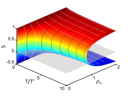
Figure 1: Equilibrium order parameter $S$ as a function of dimensionless temperature and density for the combined Maier-Saupe and modified Onsager theory [5]. $T^{\prime}=\frac{U_{0}b}{kD}$ and $\rho_{n}=\frac{1}{5}\rho_{0}D$, where $U_{0}$ fixes the energy scale and $\rho_{0}$ is the number density (see (3) and (19), respectively, for their formal definition).

We note that a much better approximation to the excluded volume of ellipsoids is obtained for different parametrization of $C$ and $D$ in terms of aspect ratio [4].

3 Attractive and repulsive interactions in the high density limit

In this section, we look into the behavior of the system near the high density limit. We begin by outlining the building blocks of our model.

We consider a one-component system consisting of hard ellipsoids interacting pairwise via both attractive and repulsive potentials. The configurational Helmholtz free energy of a system of $N$ particles, within an additive constant, is

$$F=-kT\ln\frac{1}{N!}\int_{\Omega^{N}}e^{-\frac{1}{kT}\sum_{1\leq i<j\leq N}U_{ij}}d\mathbf{q}_{1}\cdots d\mathbf{q}_{N},$$ (4)

where $k$ is the Boltzmann constant, $\mathbf{q}_{i}$ is the generalized (orientational and positional) coordinate of the $i^{th}$ particle, and $U_{ij}=U(\mathbf{q}_{i},\mathbf{q}_{j})$ is the total interaction energy between particles $i$ and $j$, the sum is over all pairs of particles.

The interaction potential consists of a long range attractive and a short range repulsive part;

$$U(\mathbf{q}_{i},\mathbf{q}_{j})=U^{A}(\mathbf{q}_{i},\mathbf{q}_{j})+U^{R}(\mathbf{q}_{i},\mathbf{q}_{j}).$$ (5)

The attractive interaction potential is of the form [5],

$$U^{A}(\mathbf{q}_{i},\mathbf{q}_{j})=-\frac{K}{r^{6}}(\bm{\alpha}_{i}:\bm{\alpha}_{j}+3\operatorname{tr}\bm{\alpha}_{i}\operatorname{tr}\bm{\alpha}_{j}),$$ (6)

where $\bm{\alpha}$ is a polarizability tensor, $\operatorname{tr}$ denotes the trace, $K>0$ is an interaction constant, and $r$ is the separation between the centers of particles. The repulsive interaction has the form

$$U^{R}(\mathbf{q}_{i},\mathbf{q}_{j})=\left\{\begin{array}[c]{l}\infty\text{, if particles interpenetrate,}\\ 0,\text{ otherwise.}\end{array}\right.$$ (7)

We write

$$G_{N}=\int_{\Omega^{N}}e^{-\frac{1}{kT}\sum_{1\leq i<j\leq N}U_{ij}}d\mathbf{q}_{1}\cdots d\mathbf{q}_{N},$$ (8)

where quantity $G_{N}$ can be thought of as the number of states available to $N$ distinguishable particles.

Since all particles are equivalent, we write, as in [4], in the spirit of mean field theory,

$$G_{N}=\left\langle\int_{\Omega}e^{-\frac{1}{kT}(\sum_{j=2}^{N}U_{1j}^{A}+\sum_{j=2}^{N}U_{1j}^{R})}d\mathbf{q}_{1}\right\rangle^{N},$$ (9)

where the average $\left\langle\cdot\right\rangle$ is calculated with respect to the $(N-1)$-particle Gibbs distribution. We further pursue our mean-field strategy, by replacing the attractive part of the potential in Eq. (9) by the single particle pseudopotential,

$$U^{A}(\mathbf{q}_{1})=\sum_{j=2}^{N}U_{1j}^{A}=\frac{1}{2}\int\rho(\mathbf{q}_{2})U_{12}^{A}(\mathbf{q}_{1},\mathbf{q}_{2})d\mathbf{q}_{2},$$ (10)

where $\rho(\mathbf{q}_{2})$ is the number density of particles with generalized coordinate $\mathbf{q}_{2}$. According to common folklore, the factor $\frac{1}{2}$ has been introduced in (10)to avoid “double counting” of particles; more precisely, its role is keeping the total attractive energy unchanged in passing from the discrete to a continuum representation:

$$\frac{1}{2}\sum_{i\neq j=1}^{N}U^{A}_{ij}=\int_{\Omega}\rho(\mathbf{q}_{1})U^{A}(\mathbf{q}_{1})d\mathbf{q}_{1}.$$ (11)

We thus rewrite (9) as

$$G_{N}=\left\langle\int_{\Omega}e^{-\frac{1}{kT}[U^{A}(\mathbf{q}_{1})+\sum_{j=2}^{N}U_{1j}^{R}]}d\mathbf{q}_{1}\right\rangle^{N},$$ (12)

where, despite $U^{A}$ being now a singe-particle function, the average $\left\langle\cdot\right\rangle$ is still computed with respect to the $(N-1)$-particle Gibbs distribution. A further step in the way of simplifying our theory is posing

$$G_{N}=\left(\int_{\Omega}e^{-\frac{1}{kT}U^{A}(\mathbf{q}_{1})}[1-W(\mathbf{q}_{1})]d\mathbf{q}_{1}\right)^{N},$$ (13)

where

$$W(\mathbf{q}_{1})=\left\langle 1-e^{-\frac{1}{kT}\Sigma_{j=2}^{N}U_{1j}^{R}}\right\rangle$$ (14)

is the average excluded volume fraction. We estimate this quantity as

$$W(\mathbf{q}_{1})=\lambda\int_{\Omega}\rho(\mathbf{q}_{2})\left[1-e^{-\frac{U^{R}(\mathbf{q}_{1},\mathbf{q}_{2})}{kT}}\right]d\mathbf{q}_{2},$$ (15)

where, as shown in [4], $\lambda$ has the role of a dimensionless phenomenological parameter.

The free energy then becomes

$$F=-kT\ln\frac{1}{N!}\left(\int_{\Omega}e^{-\frac{1}{kT}U^{A}(\mathbf{q}_{1}\mathbf{)}}[1-W(\mathbf{q}_{1})]d\mathbf{q}_{1}\right)^{N},$$ (16)

which is the cornerstone of our model. The integral in Eq. (16) can be regarded as the weighted fraction of the total volume available to particle $1$, or the weighted free volume fraction.

This can be written in the density functional form, using the procedure we developed previously as described in [5, 4],

$$F =kT\int_{\Omega}\rho(\mathbf{q}_{1})\ln\rho(\mathbf{q}_{1})d\mathbf{q}_{1}\mathbf{+}\int_{\Omega}\rho(\mathbf{q}_{1}\mathbf{)}U^{A}(\mathbf{q}_{1}\mathbf{)}d\mathbf{q_{1}}$$

$$-kT\int_{\Omega}\rho(\mathbf{q}_{1})\ln\left(1-\lambda\int_{\Omega}\rho(\mathbf{q}_{2})\left[1-e^{-\frac{1}{kT}U^{R}(\mathbf{q}_{1},\mathbf{q}_{2})}\right]d\mathbf{q}_{2}\right)d\mathbf{q}_{1}.$$ (17)

It is convenient to write the generalized coordinates in terms of position and orientation, then

$$F =kT\int_{\mathbb{S}^{2}}\int_{\mathcal{B}}\rho(\mathbf{r}_{1},\mathbf{\hat{l}}_{1})\ln\rho(\mathbf{r}_{1},\mathbf{\hat{l}}_{1})d^{3}\mathbf{r}_{1}d^{2}\mathbf{\hat{l}}_{1}\mathbf{+}\int_{\Omega}\rho(\mathbf{r}_{1},\mathbf{\hat{l}}_{1}\mathbf{)}U^{A}(\mathbf{r}_{1},\mathbf{\hat{l}}_{1}\mathbf{)}d^{3}\mathbf{r}_{1}d^{2}\mathbf{\hat{l}}_{1}$$

$$-kT\int_{\mathbb{S}^{2}}\int_{\mathcal{B}}\rho(\mathbf{r}_{1},\mathbf{\hat{l}}_{1})\ln\left(1-\lambda\int_{\mathbb{S}^{2}}\int_{\mathcal{B}}\rho(\mathbf{r}_{2},\mathbf{\hat{l}}_{2})\left[1-e^{-\frac{1}{kT}U^{R}(\mathbf{r}_{1},\mathbf{\hat{l}}_{1},\mathbf{r}_{2},\mathbf{\hat{l}}_{2})}\right]d^{3}\mathbf{r}_{2}d^{2}\mathbf{\hat{l}}_{2}\right)d^{3}\mathbf{r}_{1}d^{2}\mathbf{\hat{l}}_{1},$$ (18)

where $\rho(\mathbf{r},\mathbf{\hat{l}})$ is the number density of particles at $\mathbf{r}$ with orientation $\mathbf{\hat{l}}$. $\mathbb{S}^{2}$ denotes orientation space, the surface of the unit sphere. $\mathcal{B}$ denotes position space, occupied by particles. In a homogeneous system, the density is independent of $\mathbf{r}$, so we write

$$\rho(\mathbf{r},\mathbf{\hat{l}})=\rho_{0}f(\mathbf{\hat{l}}),$$ (19)

where $\rho_{0}$ now is simply the number density of particles, and $f(\mathbf{\hat{l}})$ is the single particle orientational distribution function satisfying

$$\int_{\mathbb{S}^{2}}f(\mathbf{\hat{l}})d^{2}\mathbf{\hat{l}}=1.$$ (20)

Integrating Eq. (3) over $\mathbf{r}_{1}$ and $\mathbf{r}_{2}$ gives

$$F =kT\rho_{0}V\left\{\ln\rho_{0}+\int_{\mathbb{S}^{2}}f(\mathbf{\hat{l}}_{1})\ln f(\mathbf{\hat{l}}_{1})d^{2}\mathbf{\hat{l}}_{1}\mathbf{+}\frac{1}{kT}\int_{\mathbb{S}^{2}}f(\mathbf{\hat{l}}_{1})U^{A}(\mathbf{\hat{l}}_{1})d^{2}\mathbf{\hat{l}}_{1}\right.$$

$$\left.-\int_{\mathbb{S}^{2}}f(\mathbf{\hat{l}}_{1})\ln\left(1-\lambda\rho_{0}\int_{\mathbb{S}^{2}}f(\mathbf{\hat{l}}_{2})V_{exc}(\mathbf{\hat{l}}_{1},\mathbf{\hat{l}}_{2})d^{2}\mathbf{\hat{l}}_{2}\right)d^{2}\mathbf{\hat{l}}_{1}\right\},$$ (21)

where

$$V_{exc}(\mathbf{\hat{l}}_{1},\mathbf{\hat{l}}_{2})=\int_{\mathcal{B}}\left[1-e^{-\frac{1}{kT}U^{R}(\mathbf{r}_{1},\mathbf{l}_{1},\mathbf{r}_{2},\mathbf{l}_{2})}\right]d^{3}\mathbf{r}$$ (22)

is excluded volume of two particles (integrated in their relative position $\mathbf{r}=\mathbf{r}_{2}-\mathbf{r}_{1}$).

If $\rho_{0}$ is small, one can expand the logarithm and recover the theory in the dilute limit [5]. We note that the expansion is only valid when

$$\lambda\rho_{0}\int_{\mathbb{S}^{2}}f(\mathbf{\hat{l}}_{2})V_{exc}(\mathbf{\hat{l}}_{1},\mathbf{\hat{l}}_{2})d^{2}\mathbf{\hat{l}}_{2}<1,$$ (23)

since the argument of logarithm must be positive.

To capture accurately the phase behavior, we keep the full logarithmic dependence in this work; this is the salient feature of our approach. This form of the free energy is the origin of a remarkable phenomenon: without the attractive interaction, above a critical value of $\rho_{0}$, the equilibrium distribution function $f(\mathbf{\hat{l}})$ is zero on a region of the orientation space with positive measure; that is, at high densities, some regions of orientation space are not accessible to particles.

Since London dispersion is a function of the particle polarizability tensor $\bm{\alpha}$, which is linear in the orientation descriptor $\bm{\sigma}(\mathbf{l})$, we can write the attractive interaction explicitly as follows [5],

$$U^{A}(\mathbf{l}_{1}) =\frac{1}{2}\int\rho(\mathbf{r}_{2},\mathbf{\hat{l}}_{2})U^{A}(\mathbf{r}_{1},\mathbf{\hat{l}}_{1},\mathbf{r}_{2},\mathbf{\hat{l}}_{2})d^{3}\mathbf{r}_{2}d\mathbf{\hat{l}}_{2}$$

$$=-\frac{1}{2}\rho_{0}U_{0}\left(a+b\frac{2}{3}\bm{\sigma}\mathbf{(\hat{l}}_{1}):\mathbf{Q}\right),$$ (24)

where $U_{0}$ is an energy (appropriately related to $K$ in (6)), and $a$ and $b$, the isotropic and anisotropic parameters of the potential, have units of volume.

Substitution of the attractive interaction (3) and the excluded volume (1) gives the free energy density (per unit volume),

$$\mathcal{F}= kT\rho_{0}\left\{\ln\rho_{0}+\int_{\mathbb{S}^{2}}f(\mathbf{\hat{l}})\ln f(\mathbf{\hat{l}})d^{2}\mathbf{\hat{l}}-\frac{1}{2kT}\int_{\mathbb{S}^{2}}f(\mathbf{\hat{l}})\rho_{0}U_{0}\left(a+b\frac{2}{3}\bm{\sigma}\mathbf{(\hat{l}):Q}\right)d^{2}\mathbf{\hat{l}}\right.$$

$$\left.-\int_{\mathbb{S}^{2}}f(\mathbf{\hat{l}})\ln\left[1-\rho_{0}\left(c-d\frac{2}{3}\bm{\sigma}\mathbf{(\hat{l})}:\mathbf{Q}\right)\right]d^{2}\mathbf{\hat{l}}\right\},$$ (25)

where

$$\mathbf{Q}=\int_{\mathbb{S}^{2}}\bm{\sigma}\mathbf{(\hat{l})}f(\mathbf{\hat{l}})d^{2}\mathbf{\hat{l},}$$ (26)

is the symmetric and traceless tensor, which is the familiar orientational order descriptor of nematic liquid crystals. Here the excluded volume constants are defined as $c=\lambda C$ and $d=\lambda D$. Note that if $f(\mathbf{\hat{l}})$ is admissible, it must satisfy

$$1-\rho_{0}\left(c+d\frac{2}{3}\bm{\sigma}\mathbf{(\hat{l})}:\mathbf{Q}\right)>0,$$ (27)

for all $\mathbf{\hat{l}}$ with $f(\mathbf{\hat{l}})>0$; that is, if the argument of the logarithm is negative, then $f(\mathbf{\hat{l}})$ must be zero.

It is convenient to introduce an auxiliary dimensionless parameter as in [4],

$$\phi=\frac{\rho_{0}c-1}{\rho_{0}d}\in(-\infty,1],$$ (28)

which is an increasing function of number density $\rho_{0}=\frac{1}{c-d\phi}$. In the very dilute limit, $\rho_{0}\rightarrow 0^{+},\phi\rightarrow-\infty$; in the dense packing limit, $\rho_{0}\rightarrow\left(\frac{1}{c-d}\right)^{-},\phi\rightarrow 1^{-}$, this corresponds to the densest packing fraction. It is remarkable that the information of the particle shape is completely subsumed in the effective density $\phi$. Retaining only relevant terms, we express the free energy density $\mathcal{F}$ in the following form

$$\mathcal{F}=kT\rho_{0}\int_{\mathbb{S}^{2}}\left[f(\mathbf{\hat{l}})\ln f(\mathbf{\hat{l}})-\tau f(\mathbf{\hat{l})}\left(\frac{a}{b}+\frac{2}{3}\bm{\sigma}\mathbf{(\hat{l}):Q}\right)-f(\mathbf{\hat{l}})\ln\left(\frac{2}{3}\bm{\sigma}(\mathbf{\hat{l}):Q}-\phi\right)\right]d^{2}\mathbf{\hat{l}},$$ (29)

where the dimensionless parameter,

$$\mathbf{\tau}=\frac{\rho_{0}U_{0}b}{kT},$$ (30)

plays the role of an effective inverse temperature. More explicitly, Eq. (29) can also be written as

$$\mathcal{F}= kT\rho_{0}\int_{\mathbb{S}^{2}}\left[f(\mathbf{\hat{l}}_{1})\ln f(\mathbf{\hat{l}}_{1})-\frac{1}{2}\tau f(\mathbf{\hat{l}}_{1})\left(\frac{a}{b}+\frac{2}{3}\bm{\sigma}(\mathbf{\hat{l}}_{1}):\int_{\mathbb{S}^{2}}\bm{\sigma}\mathbf{(\hat{l}}_{2}\mathbf{)}f(\mathbf{\hat{l}}_{2})d^{2}\mathbf{\hat{l}}_{2}\right)\right.$$

$$\left.-f(\mathbf{\hat{l}}_{1})\ln\left(\frac{2}{3}\bm{\sigma}\mathbf{(\hat{l}}_{1}):\int_{\mathbb{S}^{2}}\bm{\sigma}\mathbf{(\hat{l}}_{2}\mathbf{)}f(\mathbf{\hat{l}}_{2})d^{2}\mathbf{\hat{l}}_{2}-\phi\right)\right]d^{2}\mathbf{\hat{l}}_{1}.$$ (31)

We next minimize the free energy density (3) with respect to the orientational distribution function $f(\mathbf{\hat{l}})$. There are two constraints. First, the distribution function is normalized to unity subject to $f(\mathbf{\hat{l}})\geq 0$. Second, the argument of the logarithm, the free volume fraction, must be positive where $f(\mathbf{\hat{l}})>0$; that is,

$$\frac{2}{3}\bm{\sigma}\mathbf{(\hat{l})}:\mathbf{Q}-\phi>0.$$ (32)

Setting the first variation to zero and solving for the distribution function gives the self-consistent equation for $f$ in terms of the order parameter tensor $\mathbf{Q}$

$$f(\mathbf{\hat{l}}_{1})=\left\{\begin{array}[c]{cc}\displaystyle\frac{\left(\frac{2}{3}\bm{\sigma}\mathbf{(\hat{l}}_{1}\mathbf{)}:\mathbf{Q}-\phi\right)e^{\bm{\sigma}(\mathbf{\hat{l}}_{1}):\left(\tau\frac{2}{3}\mathbf{Q}+\displaystyle\int_{\mathbb{S}^{2}}f(\mathbf{\hat{l}}_{2})\frac{\frac{2}{3}\bm{\sigma}\mathbf{(\hat{l}}_{2})}{\frac{2}{3}\bm{\sigma}(\mathbf{\hat{l}}_{2}):\mathbf{Q}-\phi}d^{2}\mathbf{\hat{l}}_{2}\right)}}{\displaystyle\int_{\mathbb{S}^{2}}\left(\frac{2}{3}\bm{\sigma}\mathbf{(\hat{l}}_{1}\mathbf{)}:\mathbf{Q}-\phi\right)e^{\bm{\sigma}(\mathbf{\hat{l}}_{1}):\left(\tau\frac{2}{3}\mathbf{Q}+\displaystyle\int_{\mathbb{S}^{2}}f(\mathbf{\hat{l}}_{2})\frac{\frac{2}{3}\bm{\sigma}\mathbf{(\hat{l}}_{2})}{\frac{2}{3}\bm{\sigma}(\mathbf{\hat{l}}_{2}):\mathbf{Q}-\phi}d^{2}\mathbf{\hat{l}}_{2}\right)}}&\text{if }\frac{2}{3}\bm{\sigma}\mathbf{(\hat{l}):Q}-\phi>0,\\ 0&\text{otherwise}.\end{array}\right.$$ (33)

We define an auxiliary order parameter tensor $\mathbf{\Psi}$ as

$$\mathbf{\Psi}=\tau\frac{2}{3}\mathbf{Q}+\int_{\mathbb{S}^{2}}f(\mathbf{\hat{l}})\frac{\frac{2}{3}\bm{\sigma}\mathbf{(\hat{l}})}{\frac{2}{3}\bm{\sigma}\mathbf{(\hat{l})}:\mathbf{Q}-\phi}d^{2}\mathbf{\hat{l}.}$$ (34)

Finally, the equation for the orientational distribution function becomes

$$f(\mathbf{\hat{l}})=\frac{\left(\frac{2}{3}\bm{\sigma}\mathbf{(\hat{l}):Q}-\phi\right)e^{\bm{\sigma}\mathbf{(\hat{l}):\Psi}}}{\displaystyle\int_{\mathbb{S}^{2}}\left(\frac{2}{3}\bm{\sigma}\mathbf{(\hat{l}):Q}-\phi\right)e^{\bm{\sigma}\mathbf{(\hat{l}):\Psi}d^{2}\mathbf{\hat{l}}}},$$ (35)

where

$$\mathbf{Q} =\left\langle\bm{\sigma}\mathbf{(\hat{l})}\right\rangle,$$ (36a)

$$\mathbf{\Psi} =\tau\frac{2}{3}\mathbf{Q}+\left\langle\frac{\frac{2}{3}\bm{\sigma}(\mathbf{\hat{l}})}{\frac{2}{3}\bm{\sigma}\mathbf{(\hat{l})}:\mathbf{Q}-\phi}\right\rangle,$$ (36b)

with both averages $\left\langle\cdot\right\rangle$ now computed with respect to $f$ itself, as is customary in any mean-field approach. The requirement of nonnegativity of the free volume fraction, $\frac{2}{3}\mathbf{\sigma(\hat{l})}:\mathbf{Q}-\phi>0$, results in the orientational distribution function being zero in some regions of orientation space in the absence of attractive interactions [4].

The singular nature of the model makes suspect the use of the first variation to obtain the Euler-Lagrange equation (33), as it is unclear whether the free energy density is sufficiently differentiable for variations to be taken, where the orientation distribution function is zero, and whether finite-energy configurations even exist. However, by means of a duality argument, these analytical issues of models such as ours have been rigorously addressed previously [6]. In fact, the auxiliary order parameter tensor $\mathbf{\Psi}$ arises as, in a sense, a dual to the order parameter tensor $\mathbf{Q}$, though its physical interpretation still remains elusive. The analysis proves rigorously that the formal Euler-Lagrange equation (33) is indeed satisfied by equilibria for $\phi<1$, while for $\phi\geq 1$ no finite energy configurations exist, which we interpret to be the saturation limit of the model. Similar questions of differentiability can be asked of the derivation of the equation of state (see Eq. (38) below), however our formal calculation presented in this work can similarly be shown to be valid.

To derive the equation of state of our system of hard ellipsoids, we start with the relation between the pressure and the free energy density,

$$P=-\mathcal{F+}\rho_{0}\frac{\partial\mathcal{F}}{\partial\rho_{0}},$$ (37)

which gives

$$P+\frac{1}{2}\rho_{0}^{2}U_{0}\left(a+b\frac{2}{3}\mathbf{Q}^{2}\right)=\rho_{0}kT\left(\frac{1}{1-\rho_{0}c}\right)\left\langle\frac{1}{1-\frac{2}{3}\phi^{-1}\mathbf{Q}:\mathbf{\sigma(\hat{l})}}\right\rangle.$$ (38)

The denominator of the second term on the right hand side of Eq. (38)is the isotropic part of the excluded volume fraction, while the third term, the anisotropic contribution, is the reciprocal of the harmonic mean of the excluded volume fraction.

If $\mathbf{Q}=\bm{0}$, then we have

$$P+\frac{1}{2}\rho_{0}^{2}U_{0}a=\frac{\rho_{0}kT}{1-\rho_{0}c},$$ (39)

as in the Van der Waals case. In general, Eq. (38) is our equation of state. In high density regime, when $\phi$ approaches $1$, the pressure approaches infinity.

4 The assumption of uniaxiality

Without external fields, the classical models, Maier-Saupe theory [1] for attractive interactions and Onsager theory [2] for steric interactions, predict only uniaxial nematic order at high densities [7]. Here we also assume that $\mathbf{Q}$ is uniaxial to simplify the presentation. There might also be biaxial equilibrium solutions, like those found for the fully repulsive case in [4]; there, biaxial solutions were saddle points of the free energy. We expect that biaxial solutions, if they exist, would not be stable when attractive interactions are included. We write

$$\mathbf{Q}=\frac{S}{2}(3\mathbf{\hat{n}\hat{n}-I}),$$ (40)

where $S$ is the scalar order parameter and $\mathbf{\hat{n}}$ is the nematic director. One can show then that $\mathbf{\Psi}$ is also uniaxial, and shares the same eigenframe with $\mathbf{Q}$ [6], thus can be written as

$$\mathbf{\Psi}=\Psi(\mathbf{\hat{n}\hat{n}}-\frac{1}{3}\mathbf{I}).$$ (41)

Then we have

$$\mathbf{Q} :\bm{\sigma}(\mathbf{\hat{l}})\mathbf{=}\frac{3S}{2}P_{2}(\mathbf{\hat{n}}\cdot\mathbf{\hat{l}}),$$

$$\mathbf{\Psi} :\bm{\sigma}(\mathbf{\hat{l}})=\Psi P_{2}(\mathbf{\hat{n}}\cdot\mathbf{\hat{l}}),$$ (42)

where $P_{2}(x)$ is the second order Legendre polynomial. The free energy density becomes

$$\mathcal{F}=2\pi\rho_{0}kT\left(\Psi S-\frac{1}{2}\tau(\frac{a}{b}+S^{2})-\ln\int_{\mathbb{S}_{+}^{2}}(SP_{2}(x)-\phi)e^{\Psi P_{2}(x)}dx\right),$$ (43)

where use of (30) has been made, $x=\mathbf{\hat{n}\cdot\hat{l}}=\cos\theta$, and $\mathbb{S}_{+}^{2}=\{x:SP_{2}(x)-\phi>0\}$. The uniaxiality assumption makes the analysis and numerics more tractable. The distribution function is now given by

$$f(x)=\left\{\begin{array}[c]{cc}\frac{\left(SP_{2}(x)-\phi\right)\exp(\Psi P_{2}(x))}{\int_{\mathbb{S}_{+}^{2}}\left(SP_{2}(x)\mathbf{-}\phi\right)\exp(\Psi P_{2}(x))dx}&\text{if }SP_{2}(x)-\phi>0,\\ 0&\text{otherwise}.\end{array}\right.\text{ }$$ (44)

Instead of solving the above self-consistency equation for $f(x)$, we solve the coupled equations for $\Psi$ and $S$,

$$S=\frac{\int_{\mathbb{S}_{+}^{2}}P_{2}(x)\left(SP_{2}(x)-\phi\right)\exp(\Psi P_{2}(x))dx}{\int_{\mathbb{S}_{+}^{2}}\left(SP_{2}(x)\mathbf{-}\phi\right)\exp(\Psi P_{2}(x))dx}=\left\langle P_{2}(x)\right\rangle,$$ (45a)

$$\Psi=\tau S+\frac{\int_{\mathbb{S}_{+}^{2}}P_{2}(x)\exp(\Psi P_{2}(x))dx}{\int_{\mathbb{S}_{+}^{2}}\left(SP_{2}(x)-\phi\right)\exp(\Psi P_{2}(x))dx}=\tau S+\left\langle\frac{P_{2}(x)}{SP_{2}(x)-\phi}\right\rangle.$$ (45b)

Explicitly, the integration limits are

$$(x_{0},1),\text{ if }S>0\quad\text{and}\quad(0,x_{0}),\text{ if }S<0,$$ (46)

and $x_{0}>0$ is such that $P_{2}(x_{0})=\phi/S$.

For a given effective density $\phi$ and effective inverse temperature $\tau$, Eqs. (45a) and (45b) can be solved numerically for the scalar order parameters $S$ and $\Psi$, as well as for the cutoff parameter $x_{0}$; the details of the algorithm will given elsewhere. Once these are determined, the behavior of the system is known. We present the results in the following section.

5 Results

The behavior of the system without attractive interactions has been detailed in [4]. The equilibrium uniaxial order parameter $S$ versus effective density $\phi$ is shown in Fig. 2 below. The stability of different branches is determined by examining the local convexity of the free energy density. For $\phi<\phi_{NI}\approx-0.224$, the system is in the isotropic state with $S=0$; at $\phi=\phi_{NI}$, the system undergoes a first order transition to the nematic state, with order parameter $S_{NI}\approx 0.545$. As $\phi\rightarrow 1$, the order parameter $S\rightarrow 1$, indicating a completely aligned state. At $\phi=-0.2$, the vertical red line (dark gray) indicates that all values of $0.2<S<0.4$ share the same energy, corresponding to an orbit of degenerate critical points of the free energy. The two dashed lines emanating from the origin mark the boundary of the triangular region where the orientational distribution functions corresponding to equilibrium solutions do not have compact support, those outside this region do.

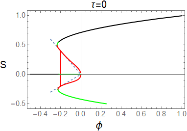
Figure 2: Equilibrium order parameter $S$ vs. $\phi$ for the solutions of the uniaxial self-consistent equations (45) when $\tau=0$. The black curve represents the stable branch of the bifurcation, the green curves (light gray) correspond to the metastable branches, and the red curves (dark gray) to the unstable branches.

Now we consider the effect of attractive interactions for some representative values of $\tau>0$, which are shown in Fig. 3. Due to the increased complexity of the energy profiles, for simplicity, here we do not distinguish metastable and unstable solution branches. Interestingly, as $\tau$ increases, the vertical line at $\phi=-0.2$ in Fig. 2 splits into two disjoint curves which move in opposite directions. One of these curves borders an island, which eventually collapses at the origin for $\tau\gg 1$. The outer curve, which evolves in a more interesting fashion, contains the essential phase transition information. The outer bifurcation curve admits noticeable kinks when it nears the two dashed lines emanating from the origin; this appears to be evocative of some singularity of the free energy when regions of orientation space first become inaccessible.

More specifically, when $\tau$ is relatively small, say $\tau=0.1$, the system undergoes a first order NI transition at $\phi_{NI}\approx-0.23$, with $S_{NI}\approx 0.54$, as shown in Fig. 3(a).

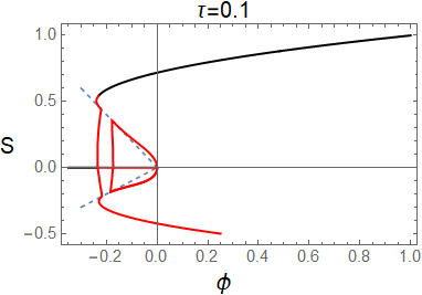
(a)

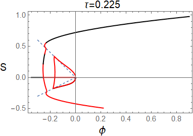
(b)

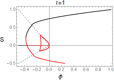
(c)

Figure 3: Equilibrium order parameter $S$ vs. $\phi$ for the solutions to the uniaxial self-consistency equations (45) with $\tau=0.1,0.225,1$, respectively. The heavy black curves represent the globally stable branch, and the red curves (dark gray, in print) represent either metastable or unstable branches.

As $\tau$ increases, both $\phi_{NI}$ and $S_{NI}$ decrease. Above a critical point $\tau\approx 0.22$, for example at $\tau=0.225$, there is a first order NI transition occurring at $\phi_{NI}\approx-0.25$ with $S_{NI}\approx 0.18$, as shown in Fig. 3(b), which is then followed by another nematic-nematic transition at $\phi_{NN}\approx-0.24$ and $S_{NN}\approx 0.53$. The sudden drop of $S_{NI}$ at the critical $\tau$ occurs when the orientational distribution function corresponding to the order parameter at the NI transition loses its compact support; the stable nematic solution now lies in between the two dashed lines in Fig. 3(b). In this region, molecular orientation far from the director is allowed. When $\tau$ is large enough, the topology of the bifurcation curves evolves further; for example, at $\tau=1$, the secondary NN transition disappears, and only the primary NI transition occurs at $\phi_{NI}\approx-0.38$ with $S_{NI}\approx 0.24$. as shown in Fig. 3(c). As $\tau$ increases further, the outer open piece of the bifurcation curve is stretched even more towards large negative values of $\phi$. At the critical value of $\tau\approx 4.488$ the leftmost point of the curve goes to $-\infty$. This means that below the critical dimensionless temperature $1/\tau\rightarrow 0.2228$, the nematic phase can exist at arbitrarily low densities $\phi$, provided the temperature is sufficiently low. The value $1/\tau=0.2228$ and the order parameter at the transition is fully consistent with Maier-Saupe theory.

The dependence of $S_{NI}$ and $\phi_{NI}$ on $\tau$ is shown in Fig. 4, which summarizes the dependence of the order parameter and critical effective density at the NI transition on temperature.

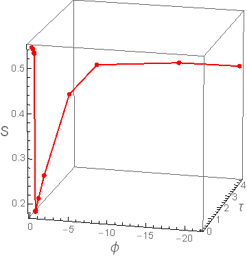
Figure 4: Equilibrium order parameter $S_{NI}$ and scaled density $\phi_{NI}$ at the isotropic-nematic transition for the solutions to the uniaxial self-consistency equations (45) plotted against the dimensionless reverse temperature $\tau$.

As the temperature decreases, the critical density and order parameter decrease slowly initially. The attractive interactions stabilize the nematic phase, the stronger the attractive interactions, the less concentration is needed to form a nematic phase. As the temperature is further decreased, the order parameter $S_{NI}$ suddenly drops at $\phi\approx 0.22$, at which point the orientational probability distribution function starts to lose its compact support and is positive everywhere in its orientational space. As the temperature is decreased beyond this point, $S_{NI}$ increases and saturates at $S_{NI}=0.43$, which agrees with the value predicted by the Maier-Saupe theory.

A preliminary study shows that if the sign of the attractive interaction is changed, the special vertical line at $\phi=-0.2$ disappears, all stable nematic equilibrium distribution functions possess compact support, and transition occurs at a higher density, order parameter values at the transition increase as the absolute value of the interaction parameter gets larger.

A more careful and complete study of the model and phase diagram is currently underway; much remains to be explained.

6 Perspectives

This paper was an attempt to combine in a unified model both attractive and repulsive sources of molecular interactions that can be responsible for the onset of nematic phases. Although this attempt was built on entirely new bases, it was not unprecedented. The need for combining these independent molecular nematogenic drives has been fueled by the weaknesses exhibited by both the Onsager and Maier-Saupe theories when applied in solitude. The former is limited by the assumption on the diluteness of particles [3]. The latter is sensitive to the assumption of spherical symmetry in the particle distribution, a small deviation from which can jeopardize the very existence of the ordering transition [8].

Perhaps the first proposal for a combined theory of repulsive and attractive interactions as driving forces for the nematic ordering of molecules goes back to Gelbart and Baron [9] (see also [10]). This theory has often been referred to as the generalized van der Waals theory; it is computationally demanding and has been explicitly applied only for special repulsive potentials. These applications had however the merit of showing clearly that the anisotropy of the mean-field potential is mostly due to the interplay between the repulsive potential and the isotropic part of the attractive potential [11, 12, 13]. For other similar models and generalized theories, the reader is referred to specialized reviews [14, 15, 16].

In a different, but concurrent vein, attractive dispersion forces have been combined with hard-core repulsion in a formal theory that has, as its crucial feature, a fourth-rank tensor, depending on the anisotropy of the interacting molecules [17] (see also Sect. 1.4 of [18]).

Finally, it is illuminating to recall the alternative approach followed by Luckhurst and Zannoni [19]. They envisaged short-range, repulsive interactions as responsible for the local organization of molecules in clusters, which in turn are subject to long-range, attractive interactions. This syncretic view posits that the molecular clusters aggregated by short-range interactions are not destroyed at the ordering transition, at which their long-range organization changes. According to this view, not molecules, but stable clusters would be subject to an effective pair potential of possible dispersion origins.

Our study was focused on the dense limit, where, in loose terms, molecules tend to form a few, highly pervasive clusters exhausting free volume. A quantitative description of this scenario is already highly problematic in the case of spherical particles with only steric interactions; various methods have been tried which may be worth combining in a unified setting [20].

Even a greater challenge lies with extending any of these methods to anisomeric hard particles. Here we were contented with showing that attractive interactions do affect the ordering transition, but in the dense limit the scene is dominated by repulsive interactions, which tend to bind all particles in a few clusters. Studying the ways that can make this happen is the objective of future research.

References

- [1] Maier W, Saupe A. Eine einfache molekulare Theorie des nematischen kristallinflüussigen Zustandes. Z Naturforsch. 1958;13a:564–566. Translated into English in [21], p. 381–385.
- [2] Onsager L. The effects of shape interaction of colloidal particles. Ann NY Acad Sci. 1949;51:627–659. Reprinted in [21], p. 625–657.
- [3] Palffy-Muhoray P, Virga EG, Zheng X. Onsager’s missing steps retraced. J Phys: Condens Matter. 2017;29(47):475102.
- [4] Nascimento ES, Palffy-Muhoray P, Taylor JM, Virga EG, Zheng X. Density functional theory for dense nematic liquid crystals with steric interactions. Phys Rev E. 2017;96:022704.
- [5] Palffy-Muhoray P, Pevnyi M, Virga EG, Zheng X. The effects of particle shape in orientationally ordered soft materials. In: Bowick MJ, Kinderlehrer D, Menon G, Radin C, editors. Mathematics and materials. (IAS/Park City Mathematics Series; Vol. 23). Providence, RI: American Mathematical Society; 2017. p. 201–253.
- [6] Taylor J. An analysis of equilibria in dense nematic liquid crystals. SIAM J Math Analysis. 2018;50(2):1918–1957.
- [7] Fatkullin I, Slastikov V. Critical points of the Onsager functional on a sphere. Nonlinearity. 2005;18(6):2565–2580.
- [8] DeJeu WH. On the role of spherical symmetry in the Maier-Saupe theory. Mol Cryst Liq Cryst. 1997;292:13–24.
- [9] Gelbart WM, Baron BA. Generalized van der Waals theory of the isotropic-nematic phase transition. J Chem Phys. 1977;66(1):207–213.
- [10] Cotter MA. Generalized van der Waals theory of nematic liquid crystals: an alternative formulation. J Chem Phys. 1977;66(10):4710–4711.
- [11] Wulf A. Short-range correlations and the effective orientational energy in liquid crystals. J Chem Phys. 1977;67(5):2254–2266.
- [12] Warner M. Interaction energies in nematogens. J Chem Phys. 1980;73(11):5874–5883.
- [13] Eldredge CP, Heath HT, Linder B, Kromhout RA. Role of dispersion potential anisotropy in the theory of nematic liquid crystals. I. The mean-field potential. J Chem Phys. 1990;92(10):6225–6234.
- [14] Singh S. Phase transitions in liquid crystals. Phys Rep. 2000;324:107–269.
- [15] Gelbart WM, Barboy B. A van der Waals picture of the isotropic-nematic liquid crystal phase transition. Acc Chem Res. 1980;13:290–296.
- [16] Gelbart WM. Molecular theory of nematic liquid crystals. J Phys Chem. 1982;86:4298–4307.
- [17] Sonnet AM, Virga EG. Steric effects in dispersion forces interactions. Phys Rev E. 2008;77:031704.
- [18] Sonnet AM, Virga EG. Dissipative ordered fluids. New York: Springer; 2012.
- [19] Luckhurst GR, Zannoni C. Why is the Maier-Saupe theory of nematic liquid crystals so successful? Nature (London). 1977;267:412–414.
- [20] Fai TG, Palffy-Muhoray P, Taylor JM, Virga EG, Zheng X. Free volume and compressibility in hard-core systems; 2018; Unpublished.
- [21] Sluckin TJ, Dunmur DA, Stegemeyer H. Crystals that flow. London, New York: Taylor & Francis; 2004.