Linear Seesaw for Dirac Neutrinos
with A4subscript𝐴4A_{4} Flavour Symmetry

Debasish Borah dborah@iitg.ac.in Department of Physics, Indian Institute of Technology Guwahati, Assam 781039, India    Biswajit Karmakar biswajit@prl.res.in Theoretical Physics Division, Physical Research Laboratory, Ahmedabad 380009, India
Abstract

We propose a linear seesaw model to realise light Dirac neutrinos within the framework of A4subscript𝐴4A_{4} discrete flavour symmetry. The additional fields and their transformations under the flavour symmetries are chosen in such a way that naturally predicts the hierarchies of different elements of the seesaw mass matrix and also keeps the unwanted terms away. For generic choices of flavon alignments, the model predicts normal hierarchical light neutrino masses with the atmospheric mixing angle in the lower octant. Apart from predicting interesting correlations between different neutrino parameters as well as between neutrino and model parameters, the model also predicts the leptonic Dirac CP phase to lie in a specific range π/2δπ/5less-than-or-similar-to𝜋2𝛿less-than-or-similar-to𝜋5-\pi/2\lesssim\delta\lesssim-\pi/5 and π/5δπ/2less-than-or-similar-to𝜋5𝛿less-than-or-similar-to𝜋2\pi/5\lesssim\delta\lesssim\pi/2 that includes the currently preferred maximal value. The predictions for the absolute neutrino masses in one specific version of the model can also saturate the cosmological upper bound on sum of absolute neutrino masses.

I Introduction

The fact that neutrinos have non-zero but tiny masses, several order of magnitudes smaller compared to the electroweak scale and large mixing Patrignani et al. (2016) has been verified again and again in the last two decades. The present status of neutrino oscillation data can be found in the recent global fit analysis Esteban et al. (2017); de Salas et al. (2017); nuf , which clearly indicate that we do not yet know some of the neutrino parameters namely, the mass hierarchy of neutrinos: normal (m3>m2>m1)subscript𝑚3subscript𝑚2subscript𝑚1(m_{3}>m_{2}>m_{1}) or inverted (m2>m1>m3)subscript𝑚2subscript𝑚1subscript𝑚3(m_{2}>m_{1}>m_{3}), leptonic CP violation as well as the octant of atmospheric mixing angle θ23subscript𝜃23\theta_{23}. While the next generation neutrino experiments will be able to settle these issues, one still can not determine the nature of neutrino: Dirac or Majorana in neutrino oscillation experiments. Though Majorana nature of neutrinos can be probed through lepton number violating signatures like neutrinoless double beta decay (0νββ)0𝜈𝛽𝛽(0\nu\beta\beta), there has not been any positive signal of it yet. For example, please refer to the latest results from KamLAND-ZEN experiment Gando et al. (2016). Although such null results only disfavour the quasi-degenerate regime of light Majorana neutrinos and can never rule out Majorana nature of neutrinos, this has recently motivated the particle physics community to study the scenario of Dirac neutrinos with similar interest as given to Majorana neutrinos in the last few decades. The conventional seesaw mechanism for the origin of neutrino masses Minkowski (1977); Gell-Mann et al. (1979); Mohapatra and Senjanovic (1980); Schechter and Valle (1980) and its many descendants predict light Majorana neutrinos. On the contrary, there were fewer proposals to generate light Dirac neutrino masses initially Babu and He (1989); Peltoniemi et al. (1993) but it has recently gained momentum with several new proposals to realise sub-eV scale Dirac neutrino masses Centelles Chuliá et al. (2017a); Aranda et al. (2014); Chen et al. (2016); Ma et al. (2015); Reig et al. (2016); Wang and Han (2016); Wang et al. (2017, 2006); Gabriel and Nandi (2007); Davidson and Logan (2009, 2010); Bonilla and Valle (2016); Farzan and Ma (2012); Bonilla et al. (2016); Ma and Popov (2017); Ma and Sarkar (2018); Borah (2016); Borah and Dasgupta (2016); Borah and Dasgupta (2017a, b); Centelles Chuliá et al. (2017b); Bonilla et al. (2018); Memenga et al. (2013); Borah and Karmakar (2018); Centelles Chuliá et al. (2018a, b); Han and Wang (2018); Borah et al. (2018). Since the coupling of left and right handed neutrinos to the standard model (SM) Higgs field will require fine tuning of Yukawa coupling to the level of 1012superscript101210^{-12} or even less, it is important to forbid such couplings at tree level by introducing some additional symmetries such as U(1)BL,ZN,A4𝑈subscript1𝐵𝐿subscript𝑍𝑁subscript𝐴4U(1)_{B-L},Z_{N},A_{4} which also make sure that the right handed singlet neutrinos do not acquire any Majorana mass terms.

There have been several discussions on other conventional seesaw mechanisms in the context of Dirac neutrinos for example, type I seesaw Centelles Chuliá et al. (2017b); Borah and Karmakar (2018), type II seesaw Bonilla et al. (2018), inverse seesaw Borah and Karmakar (2018) and so on. Here show how light Dirac neutrinos can be realised within another seesaw scenario, known as linear seesaw mechanism. We consider the presence of A4subscript𝐴4A_{4} flavour symmetry augmented by additional discrete ZNsubscript𝑍𝑁Z_{N} and global lepton number symmetries which not only dictate the neutrino mixing patterns but also keep the unwanted terms away from the seesaw mass matrix, in order to realise linear seesaw. Linear seesaw for Majorana neutrino was proposed in earlier works Malinsky et al. (2005); Hirsch et al. (2009) and further extended to radiative seesaw models in Wang and Han (2015); Das et al. (2017) and hidden gauge sector models in Nomura and Okada (2018). We extend it to Dirac neutrino scenarios in a minimal way incorporating the above-mentioned flavour symmetries. Apart from retaining the usual attractive feature of linear seesaw, like the viability of seesaw scale at TeV naturally without much fine-tuning, the model also predicts several other aspects of neutrinos that can be tested at upcoming experiments. Among them, the preference for normal hierarchy, specific range of Dirac CP phase that includes the maximal value, atmospheric mixing angle in lower octant are the ones which address the present puzzles in neutrino physics.

Rest of the paper is organised as follows. In section II, we discuss the conventional and Dirac linear seesaw model and its predictions for sub-eV Dirac neutrinos in details. Finally, we conclude in section III.

II The Linear Seesaw Model

In the conventional linear seesaw model for Majorana neutrinos Malinsky et al. (2005); Hirsch et al. (2009), the standard model fermion content is effectively extended by two different types of neutral singlet fermions (N,S)𝑁𝑆(N,S) per generation and the complete neutral fermion mass matrix (9×9999\times 9) in the basis (νL,N,Ssubscript𝜈𝐿𝑁𝑆\nu_{L},N,S) assumes the form

Mν=(0mDMLmDT0MMLTMT0),subscript𝑀𝜈0subscript𝑚𝐷subscript𝑀𝐿superscriptsubscript𝑚𝐷𝑇0𝑀superscriptsubscript𝑀𝐿𝑇superscript𝑀𝑇0M_{\nu}=\left(\begin{array}[]{ccc}0&m_{D}&M_{L}\\ m_{D}^{T}&0&M\\ M_{L}^{T}&M^{T}&0\end{array}\right), (1)

due to the chosen symmetries or scalar content of the model. The light neutrino mass matrix can be derived from this as

mν=mD(MLM1)T+(MLM1)mDT,subscript𝑚𝜈subscript𝑚𝐷superscriptsubscript𝑀𝐿superscript𝑀1𝑇subscript𝑀𝐿superscript𝑀1superscriptsubscript𝑚𝐷𝑇m_{\nu}=m_{D}(M_{L}M^{-1})^{T}+(M_{L}M^{-1})m_{D}^{T}, (2)

which, being linear in Dirac neutrino mass matrix mDsubscript𝑚𝐷m_{D} is known as the linear seesaw Malinsky et al. (2005); Hirsch et al. (2009). Here the effective light neutrino mass is roughly given by ϵmD/Msimilar-toabsentitalic-ϵsubscript𝑚𝐷𝑀\sim\epsilon m_{D}/M where ϵitalic-ϵ\epsilon is originated from a small lepton number violating term in MLsubscript𝑀𝐿M_{L}, the (13) entry of the neutral fermion mass matrix given in Eq. (1). This is a simple alternative to the usual inverse seesaw model Mohapatra (1986); Mohapatra and Valle (1986); Gonzalez-Garcia and Valle (1989); Catano et al. (2012) where we also introduce two sets of gauge singlet Majorana neutrinos at the TeV scale to obtain light neutrino mass in sub-eV range. We now consider an extension of this simple linear seesaw model to generate sub-eV Dirac neutrino masses following a similar roadmap that was used to accommodate light Dirac neutrinos in type I seesaw Centelles Chuliá et al. (2017b); Borah and Karmakar (2018), type II seesaw Bonilla et al. (2018), inverse seesaw Borah and Karmakar (2018) etc. Apart from introducing the right handed counterpart of the usual left handed neutrinos, the other heavy fermions introduced for seesaw purpose are of Dirac nature, having both helicities: (NL,NRsubscript𝑁𝐿subscript𝑁𝑅N_{L},N_{R}) and (SL,SRsubscript𝑆𝐿subscript𝑆𝑅S_{L},S_{R}). In such a case the complete linear seesaw mass matrix can be written in (νL,NL,SL)T,(νR,NR,SR)superscriptsubscript𝜈𝐿subscript𝑁𝐿subscript𝑆𝐿𝑇subscript𝜈𝑅subscript𝑁𝑅subscript𝑆𝑅(\nu_{L},N_{L},S_{L})^{T},(\nu_{R},N_{R},S_{R}) basis as

mν=(0mνNMνSmνN0MNSMνSMNS0).subscript𝑚𝜈0subscript𝑚𝜈𝑁subscript𝑀𝜈𝑆superscriptsubscript𝑚𝜈𝑁0subscript𝑀𝑁𝑆subscriptsuperscript𝑀𝜈𝑆subscriptsuperscript𝑀𝑁𝑆0m_{\nu}=\left(\begin{array}[]{ccc}0&m_{\nu N}&M_{\nu S}\\ m_{\nu N}^{\prime}&0&M_{NS}\\ M^{\prime}_{\nu S}&M^{\prime}_{NS}&0\end{array}\right). (3)

The corresponding formula for light Dirac neutrinos can be written as

mνsubscript𝑚𝜈\displaystyle m_{\nu} =\displaystyle= mνN(MνSMNS1)+(MνSMNS1)mνN.subscript𝑚𝜈𝑁subscriptsuperscript𝑀𝜈𝑆superscriptsubscript𝑀𝑁𝑆1subscript𝑀𝜈𝑆superscriptsubscript𝑀𝑁𝑆1subscriptsuperscript𝑚𝜈𝑁\displaystyle m_{\nu N}(M^{\prime}_{\nu S}M_{NS}^{\prime-1})+(M_{\nu S}M_{NS}^{-1})m^{\prime}_{\nu N}. (4)

Similar to the linear seesaw for Majorana neutrinos, here also if we demand the two terms mνN,MνSsubscriptsuperscript𝑚𝜈𝑁subscriptsuperscript𝑀𝜈𝑆m^{\prime}_{\nu N},M^{\prime}_{\nu S} to be small, one can generate light Dirac neutrino masses in a TeV scale linear seesaw mechanism. However, the naturalness of such small terms can not be due to an approximate lepton number symmetry, as we are considering exact global lepton number symmetry to have purely Dirac nature of light neutrinos. Therefore, we can consider another global symmetry which is approximately broken by the two terms mνN,MνSsubscriptsuperscript𝑚𝜈𝑁subscriptsuperscript𝑀𝜈𝑆m^{\prime}_{\nu N},M^{\prime}_{\nu S} which naturally makes them small according to the t’Hooft’s naturalness criterion ’t Hooft (1980). It is worth noting that both these terms contain the right handed neutrino νRsubscript𝜈𝑅\nu_{R}. Therefore under the approximate global symmetry U(1)X𝑈subscript1𝑋U(1)_{X}, say, the singlet fermion νRsubscript𝜈𝑅\nu_{R} can have some non-zero charge so that the two terms mνN,MνSsubscriptsuperscript𝑚𝜈𝑁subscriptsuperscript𝑀𝜈𝑆m^{\prime}_{\nu N},M^{\prime}_{\nu S} explicitly break this symmetry, providing a natural origin of their smallness.

Here we intend to present an A4subscript𝐴4A_{4} flavour symmetric model of Dirac linear seesaw, in a way similar to the Altarelli-Feruglio model Altarelli and Feruglio (2006) for Majorana light neutrinos. Since minimal versions of such models often involve higher dimensional operators to allow coupling of A4subscript𝐴4A_{4} flavons (which are SM singlets) and leptons, we first briefly discuss a renormalisable version of Dirac linear seesaw before discussing an A4subscript𝐴4A_{4} symmetric one in details. In order to generate the desired structure we also choose discrete symmetries Z4×Z3subscript𝑍4subscript𝑍3Z_{4}\times Z_{3}. The presence of an approximate global symmetry U(1)X𝑈subscript1𝑋U(1)_{X} is also assumed in order to naturally accommodate a TeV scale version of such seesaw. The field content and the transformations under the chosen symmetries are shown in table 1. The renormalisable Yukawa Lagrangian can be written as

Ysubscript𝑌\displaystyle\mathcal{L}_{Y} α,βYeL¯αHeβ+Y2L¯H~NR+Y3L¯H~SR+Y4νR¯NLϕ1subscript𝛼𝛽subscript𝑌𝑒subscript¯𝐿𝛼𝐻subscript𝑒𝛽subscript𝑌2¯𝐿~𝐻subscript𝑁𝑅subscript𝑌3¯𝐿~𝐻subscript𝑆𝑅subscript𝑌4¯subscript𝜈𝑅subscript𝑁𝐿subscriptitalic-ϕ1absent\displaystyle\supset\sum_{\alpha,\beta}Y_{e}\bar{L}_{\alpha}He_{\beta}+Y_{2}\bar{L}\tilde{H}N_{R}+Y_{3}\bar{L}\tilde{H}S_{R}+Y_{4}\bar{\nu_{R}}N_{L}\phi_{1}
+Y5SL¯νRϕ1+Y6SR¯NLϕ2+Y7SL¯NRϕ2+h.c.formulae-sequencesubscript𝑌5¯subscript𝑆𝐿subscript𝜈𝑅subscriptsuperscriptitalic-ϕ1subscript𝑌6¯subscript𝑆𝑅subscript𝑁𝐿subscriptitalic-ϕ2subscript𝑌7¯subscript𝑆𝐿subscript𝑁𝑅subscriptsuperscriptitalic-ϕ2hc\displaystyle+Y_{5}\bar{S_{L}}\nu_{R}\phi^{\dagger}_{1}+Y_{6}\bar{S_{R}}N_{L}\phi_{2}+Y_{7}\bar{S_{L}}N_{R}\phi^{\dagger}_{2}+{\rm h.c.} (5)

Therefore, after the SM Higgs and the singlet scalar fields acquire non-zero vacuum expectation value (vev), one can generate the Dirac linear seesaw mass matrix (3) with different terms given by

mνN=Y2H,MνS=Y3H,mνN=Y4ϕ1,formulae-sequencesubscript𝑚𝜈𝑁subscript𝑌2delimited-⟨⟩𝐻formulae-sequencesubscript𝑀𝜈𝑆subscript𝑌3delimited-⟨⟩𝐻subscriptsuperscript𝑚𝜈𝑁subscript𝑌4delimited-⟨⟩subscriptitalic-ϕ1m_{\nu N}=Y_{2}\langle H\rangle,M_{\nu S}=Y_{3}\langle H\rangle,m^{\prime}_{\nu N}=Y_{4}\langle\phi_{1}\rangle,
MνS=Y5ϕ1,MNS=Y6ϕ2,MNS=Y7ϕ2.formulae-sequencesubscriptsuperscript𝑀𝜈𝑆subscript𝑌5delimited-⟨⟩subscriptitalic-ϕ1formulae-sequencesubscript𝑀𝑁𝑆subscript𝑌6delimited-⟨⟩subscriptitalic-ϕ2subscriptsuperscript𝑀𝑁𝑆subscript𝑌7delimited-⟨⟩subscriptitalic-ϕ2M^{\prime}_{\nu S}=Y_{5}\langle\phi_{1}\rangle,M_{NS}=Y_{6}\langle\phi_{2}\rangle,M^{\prime}_{NS}=Y_{7}\langle\phi_{2}\rangle.

Now, under the approximate global symmetry U(1)X𝑈subscript1𝑋U(1)_{X} mentioned above, we can have either νRsubscript𝜈𝑅\nu_{R} or the singlet scalar ϕ1subscriptitalic-ϕ1\phi_{1} having non-trivial charge. In the case of approximate global symmetry U(1)X𝑈subscript1𝑋U(1)_{X} under which only νRsubscript𝜈𝑅\nu_{R} is charged, one can have the Yukawa couplings Y4,Y5subscript𝑌4subscript𝑌5Y_{4},Y_{5} naturally small as Y4,50subscript𝑌450Y_{4,5}\rightarrow 0 helps us recover the full global U(1)X𝑈subscript1𝑋U(1)_{X} symmetry. This also makes the terms mνN,MνSsubscriptsuperscript𝑚𝜈𝑁subscriptsuperscript𝑀𝜈𝑆m^{\prime}_{\nu N},M^{\prime}_{\nu S} naturally small, required for the realisation of a TeV scale linear seesaw. On the other hand, if ϕ1subscriptitalic-ϕ1\phi_{1} is charged under U(1)X𝑈subscript1𝑋U(1)_{X} and its mass squared term is positive definite, then it can acquire an induced vev from soft U(1)X𝑈subscript1𝑋U(1)_{X} breaking terms in the scalar potential. However, suitable scalars have to be incorporated to allow such soft U(1)X𝑈subscript1𝑋U(1)_{X} breaking terms that do not break any of the other symmetries.

The charged lepton mass is given by ml=YeHsubscript𝑚𝑙subscript𝑌𝑒delimited-⟨⟩𝐻m_{l}=Y_{e}\langle H\rangle. We also note that both Z4subscript𝑍4Z_{4} and Z3subscript𝑍3Z_{3} are required for the desired structure of the linear seesaw mass matrix. For example, if we do not have Z3subscript𝑍3Z_{3} symmetry, then for the given Z4subscript𝑍4Z_{4} charges, we can also write terms like NL¯NRϕ2,SL¯SRϕ2¯subscript𝑁𝐿subscript𝑁𝑅subscriptitalic-ϕ2¯subscript𝑆𝐿subscript𝑆𝑅subscriptitalic-ϕ2\bar{N_{L}}N_{R}\phi_{2},\bar{S_{L}}S_{R}\phi_{2} which will give non-zero contribution to the (22) and (33) entries of the linear seesaw mass matrix (3). Therefore, we retain both the discrete symmetries. Since there is no A4subscript𝐴4A_{4} or similar non-abelian discrete symmetries acting over the generation of fermions, this model does not further predict the structure of different Yukawa coupling mass matrices involved. So there exists lots of freedom in fitting the resulting light neutrino mass matrix with the neutrino oscillation data. To make the model more predictive, we now consider an A4subscript𝐴4A_{4} flavour symmetric version of Dirac linear seesaw and numerically analyse its predictions for the light neutrino sector. The price we have to pay for such minimality is to go beyond the renormalisable level thereby introducing dimension five operators. We also utilise these higher dimensional operators to explain the hierarchy between different terms of the linear seesaw mass matrix and hence do not have the requirement of any approximate global symmetry like U(1)X𝑈subscript1𝑋U(1)_{X} discussed above. It should be noted that the renormalisable versions of such seesaw mechanisms, in principle, do not necessarily require exact or approximate global symmetries like U(1)L,U(1)X𝑈subscript1𝐿𝑈subscript1𝑋U(1)_{L},U(1)_{X}. As shown in Hirsch et al. (2018), the global lepton number symmetry broken to an appropriate Znsubscript𝑍𝑛Z_{n} subgroup is enough to protect Dirac nature of neutrinos and invoke naturalness arguments justifying linear Dirac seesaw discussed above.

Fields L𝐿L eR,μR,τRsubscript𝑒𝑅subscript𝜇𝑅subscript𝜏𝑅e_{\mbox{\tiny$R$}},\mu_{\mbox{\tiny$R$}},\tau_{\mbox{\tiny$R$}} H𝐻H νRsubscript𝜈𝑅\nu_{\mbox{\tiny$R$}} NLsubscript𝑁𝐿N_{L} NRsubscript𝑁𝑅N_{\mbox{\tiny$R$}} SLsubscript𝑆𝐿S_{L} SRsubscript𝑆𝑅S_{R} ϕ1subscriptitalic-ϕ1\phi_{1} ϕ2subscriptitalic-ϕ2\phi_{2}
SU(2)L𝑆𝑈subscript2𝐿SU(2)_{L} 222 111 2 1 111 111 111 111 111 1
Z4subscript𝑍4Z_{4} i𝑖i i𝑖i 1 1 -i𝑖i i𝑖i -i𝑖i i𝑖i i𝑖i -1
Z3subscript𝑍3Z_{3} 1 1 1 ω𝜔\omega ω2superscript𝜔2\omega^{2} 1 ω2superscript𝜔2\omega^{2} 1 ω2superscript𝜔2\omega^{2} ω𝜔\omega
Table 1: Fields content and transformation properties under Z4×Z3subscript𝑍4subscript𝑍3Z_{4}\times Z_{3} discrete symmetry for renormalisable Dirac linear seesaw.

To obtain the desired structure of the seesaw mass matrix given in Eq. (3) and to obtain the required hierarchy among its elements, we consider Z4×Z3subscript𝑍4subscript𝑍3Z_{4}\times Z_{3} symmetry and a global lepton number U(1)L𝑈subscript1𝐿U(1)_{L} symmetry in addition to A4subscript𝐴4A_{4} flavour symmetry which plays a crucial role in realising flavour structures of the corresponding mass matrices.

Fields L𝐿L eR,μR,τRsubscript𝑒𝑅subscript𝜇𝑅subscript𝜏𝑅e_{\mbox{\tiny$R$}},\mu_{\mbox{\tiny$R$}},\tau_{\mbox{\tiny$R$}} H𝐻H νRsubscript𝜈𝑅\nu_{\mbox{\tiny$R$}} NLsubscript𝑁𝐿N_{L} NRsubscript𝑁𝑅N_{\mbox{\tiny$R$}} SLsubscript𝑆𝐿S_{L} SRsubscript𝑆𝑅S_{R} ϕSsubscriptitalic-ϕ𝑆\phi_{\mbox{\tiny$S$}} ϕTsubscriptitalic-ϕ𝑇\phi_{\mbox{\tiny$T$}} ξ𝜉\xi η𝜂\eta ρ𝜌\rho
SU(2)L𝑆𝑈subscript2𝐿SU(2)_{L} 2 1 2 1 1 1 1 1 1 1 1 1 1
A4subscript𝐴4A_{4} 3 1,1′′superscript1′′1^{\prime\prime},1superscript11^{\prime} 1 3 3 3 3 3 3 3 1 1 1
Z4subscript𝑍4Z_{4} i𝑖i i𝑖i 1 1 -i𝑖i i𝑖i -i𝑖i i𝑖i -111 1 -111 -1 i𝑖i
Z3subscript𝑍3Z_{3} 1 1 1 ω𝜔\omega ω2superscript𝜔2\omega^{2} 1 ω2superscript𝜔2\omega^{2} 1 ω𝜔\omega 1 ω𝜔\omega ω𝜔\omega 1
U(1)L𝑈subscript1𝐿U(1)_{L} 1 1 0 1 1 1 1 1 0 0 0 0 0
Table 2: Fields content and transformation properties under A4×Z4×Z3subscript𝐴4subscript𝑍4subscript𝑍3A_{4}\times Z_{4}\times Z_{3} symmetry for linear seesaw.

In table 2 we elaborate the transformation of SM fields as well as the additional fermions and flavons involved in the present construction of linear seesaw. Here the SM lepton doublets (L𝐿L) and the additional singlet neutral fermions transform as A4subscript𝐴4A_{4} triplets. On the other hand, SM charged leptons (eR,μR,τRsubscript𝑒𝑅subscript𝜇𝑅subscript𝜏𝑅e_{\mbox{\tiny$R$}},\mu_{\mbox{\tiny$R$}},\tau_{\mbox{\tiny$R$}}) transform as 1,1′′superscript1′′1^{\prime\prime} and 1superscript11^{\prime} respectively under same A4subscript𝐴4A_{4} symmetry. Likewise most A4subscript𝐴4A_{4} flavour models, two A4subscript𝐴4A_{4} triplet flavons present in the set-up ϕTsubscriptitalic-ϕ𝑇\phi_{\mbox{\tiny$T$}} and ϕSsubscriptitalic-ϕ𝑆\phi_{\mbox{\tiny$S$}}, play an instrumental role in generating the non-diagonal mass matrices for charged lepton and neutrino sectors respectively. The Yukawa Lagrangian upto leading order for charged leptons invariant under this A4×Z4×Z3×U(1)Lsubscript𝐴4subscript𝑍4subscript𝑍3𝑈subscript1𝐿A_{4}\times Z_{4}\times Z_{3}\times U(1)_{L} symmetry is

CLsubscriptCL\displaystyle\mathcal{L}_{\rm CL} =yeΛ(L¯ϕT)HeR+yμΛ(L¯ϕT)1HμR+yτΛ(L¯ϕT)1′′HτR+h.c.,absentsubscript𝑦𝑒Λ¯𝐿subscriptitalic-ϕ𝑇𝐻subscript𝑒𝑅subscript𝑦𝜇Λsubscript¯𝐿subscriptitalic-ϕ𝑇superscript1𝐻subscript𝜇𝑅subscript𝑦𝜏Λsubscript¯𝐿subscriptitalic-ϕ𝑇superscript1′′𝐻subscript𝜏𝑅h.c.\displaystyle=\frac{y_{e}}{\Lambda}(\bar{L}\phi_{\mbox{\tiny$T$}})He_{\mbox{\tiny$R$}}+\frac{y_{\mu}}{\Lambda}(\bar{L}\phi_{\mbox{\tiny$T$}})_{1^{\prime}}H\mu_{\mbox{\tiny$R$}}+\frac{y_{\tau}}{\Lambda}(\bar{L}\phi_{\mbox{\tiny$T$}})_{1^{\prime\prime}}H\tau_{\mbox{\tiny$R$}}+\text{h.c.}, (6)

where ΛΛ\Lambda is the cut-off scale of the theory and both y𝑦y’s are the respective dimensionless Yukawa coupling constants. Here the leading order contribution to the charged leptons via L¯Hi¯𝐿𝐻subscript𝑖\bar{L}H\ell_{i} (where isubscript𝑖\ell_{i} are the right handed charged leptons) are not invariant under A4subscript𝐴4A_{4} symmetry. In presence of the triplet flavon ϕTsubscriptitalic-ϕ𝑇\phi_{\mbox{\tiny$T$}} one can easily construct A4subscript𝐴4A_{4} invariant dimension five operators as shown on the right hand side of Eq. (6) which subsequently generate the relevant masses for charged leptons after flavon ϕTsubscriptitalic-ϕ𝑇\phi_{\mbox{\tiny$T$}} and the SM Higgs field acquire non-zero vev. In appendix A, we have briefly summarised the A4subscript𝐴4A_{4} product rules which dictate the flavour structure of the mass matrices. Now, for the triplet flavon ϕTsubscriptitalic-ϕ𝑇\phi_{\mbox{\tiny$T$}}, considering a generic vev alignment ϕT=(vT,vT,vT)delimited-⟨⟩subscriptitalic-ϕ𝑇subscript𝑣𝑇subscript𝑣𝑇subscript𝑣𝑇\langle\phi_{\mbox{\tiny$T$}}\rangle=(v_{\mbox{\tiny$T$}},v_{\mbox{\tiny$T$}},v_{\mbox{\tiny$T$}}), the charged lepton mass matrix can be written as

ml=vvTΛ(yeyμyτyeωyμω2yτyeω2yμωyτ),subscript𝑚𝑙𝑣subscript𝑣𝑇Λsubscript𝑦𝑒subscript𝑦𝜇subscript𝑦𝜏subscript𝑦𝑒𝜔subscript𝑦𝜇superscript𝜔2subscript𝑦𝜏subscript𝑦𝑒superscript𝜔2subscript𝑦𝜇𝜔subscript𝑦𝜏\displaystyle m_{l}=\frac{vv_{\mbox{\tiny$T$}}}{\Lambda}\left(\begin{array}[]{ccc}y_{e}&y_{\mu}&y_{\tau}\\ y_{e}&\omega y_{\mu}&\omega^{2}y_{\tau}\\ y_{e}&\omega^{2}y_{\mu}&\omega y_{\tau}\end{array}\right), (10)

where v𝑣v is the vev of the SM Higgs doublet H𝐻H and ω=ei2π/3𝜔superscript𝑒𝑖2𝜋3\omega=e^{i2\pi/3} is the cube root of unity. This charged lepton mass matrix now can be diagonalised by using a matrix Uωsubscript𝑈𝜔U_{\omega} (also known as the magic matrix), given by

Uω=13(1111ωω21ω2ω).subscript𝑈𝜔131111𝜔superscript𝜔21superscript𝜔2𝜔\displaystyle U_{\omega}=\frac{1}{\sqrt{3}}\left(\begin{array}[]{ccc}1&1&1\\ 1&\omega&\omega^{2}\\ 1&\omega^{2}&\omega\end{array}\right). (14)

Now, for neutrino sector the relevant Yukawa Lagrangian is given by

ν=subscript𝜈absent\displaystyle\mathcal{L}_{\nu}= YνNL¯H~NR+νR¯NL(yξ2ξ+yη2η+ys2ϕs+ya2ϕs)ρΛsubscript𝑌𝜈𝑁¯𝐿~𝐻subscript𝑁𝑅¯subscript𝜈𝑅subscript𝑁𝐿subscriptsuperscript𝑦subscript𝜉2superscript𝜉subscriptsuperscript𝑦subscript𝜂2superscript𝜂subscriptsuperscript𝑦subscript𝑠2superscriptsubscriptitalic-ϕ𝑠subscriptsuperscript𝑦subscript𝑎2superscriptsubscriptitalic-ϕ𝑠superscript𝜌Λ\displaystyle~{}~{}Y_{\nu N}\bar{L}\tilde{H}N_{R}+\bar{\nu_{\mbox{\tiny$R$}}}{N_{L}}\left(y^{\prime}_{\xi_{2}}\xi^{\dagger}+y^{\prime}_{\eta_{2}}\eta^{\dagger}+y^{\prime}_{s_{2}}\phi_{s}^{\dagger}+y^{\prime}_{a_{2}}\phi_{s}^{\dagger}\right)\frac{\rho^{\dagger}}{\Lambda}
+YνSL¯H~SR+SL¯νR(yξ1ξ+yη1η+ys1ϕs+ya1ϕs)ρΛsubscript𝑌𝜈𝑆¯𝐿~𝐻subscript𝑆𝑅¯subscript𝑆𝐿subscript𝜈𝑅subscriptsuperscript𝑦subscript𝜉1𝜉subscriptsuperscript𝑦subscript𝜂1𝜂subscriptsuperscript𝑦subscript𝑠1subscriptitalic-ϕ𝑠subscriptsuperscript𝑦subscript𝑎1subscriptitalic-ϕ𝑠𝜌Λ\displaystyle~{}~{}~{}+Y_{\nu S}\bar{L}\tilde{H}S_{R}+\bar{S_{L}}\nu_{\mbox{\tiny$R$}}\left(y^{\prime}_{\xi_{1}}\xi+y^{\prime}_{\eta_{1}}\eta+y^{\prime}_{s_{1}}\phi_{s}+y^{\prime}_{a_{1}}\phi_{s}\right)\frac{\rho}{\Lambda}
+SR¯NL(yξ2ξ+yη2η+ys2ϕs+ya2ϕs)¯subscript𝑆𝑅subscript𝑁𝐿subscript𝑦subscript𝜉2𝜉subscript𝑦subscript𝜂2𝜂subscript𝑦subscript𝑠2subscriptitalic-ϕ𝑠subscript𝑦subscript𝑎2subscriptitalic-ϕ𝑠\displaystyle~{}~{}~{}+\bar{S_{R}}N_{L}(y_{\xi_{2}}\xi+y_{\eta_{2}}\eta+y_{s_{2}}\phi_{s}+y_{a_{2}}\phi_{s})
+SL¯NR(yξ1ξ+yη1η+ys1ϕs+ya1ϕs)+h.c.¯subscript𝑆𝐿subscript𝑁𝑅subscript𝑦subscript𝜉1superscript𝜉subscript𝑦subscript𝜂1superscript𝜂subscript𝑦subscript𝑠1subscriptsuperscriptitalic-ϕ𝑠subscript𝑦subscript𝑎1subscriptsuperscriptitalic-ϕ𝑠h.c.\displaystyle~{}~{}~{}+\bar{S_{L}}N_{R}(y_{\xi_{1}}\xi^{\dagger}+y_{\eta_{1}}\eta^{\dagger}+y_{s_{1}}\phi^{\dagger}_{s}+y_{a_{1}}\phi^{\dagger}_{s})+\text{h.c.} (15)

Here both L¯H~NR¯𝐿~𝐻subscript𝑁𝑅\bar{L}\tilde{H}N_{R} and L¯H~SR¯𝐿~𝐻subscript𝑆𝑅\bar{L}\tilde{H}S_{R} terms, involving SM lepton doublet are generated at tree level. As both SM lepton doublets (L𝐿L) and gauge singlet Dirac fermions (N,S𝑁𝑆N,S) are A4subscript𝐴4A_{4} triplets (the SM Higgs H𝐻H being a singlet under the same), following the A4subscript𝐴4A_{4} multiplication rules given in appendix A, we find the associated mass matrices to be diagonal. These mass matrices can be written as

mνN=YνNv𝐈,MνS=YνSv𝐈,formulae-sequencesubscript𝑚𝜈𝑁subscript𝑌𝜈𝑁𝑣𝐈subscript𝑀𝜈𝑆subscript𝑌𝜈𝑆𝑣𝐈\displaystyle m_{\nu N}=Y_{\nu N}v\mathbf{I},~{}~{}M_{\nu S}=Y_{\nu S}v\mathbf{I}, (16)

where 𝐈𝐈\mathbf{I} is a 3×3333\times 3 identity matrix. On the other hand, owing to the specific discrete Z4×Z3subscript𝑍4subscript𝑍3Z_{4}\times Z_{3} symmetry, SLsubscript𝑆𝐿S_{L}-νRsubscript𝜈𝑅\nu_{\mbox{\tiny$R$}} and νRsubscript𝜈𝑅\nu_{\mbox{\tiny$R$}}-NLsubscript𝑁𝐿N_{L} couplings are generated at dimension five level, ensuring the smallness of these couplings. These contributions come via involvement of the A4subscript𝐴4A_{4} singlet flavons ξ,η𝜉𝜂\xi,\eta and ρ𝜌\rho as well as the triplet flavon ϕSsubscriptitalic-ϕ𝑆\phi_{\mbox{\tiny$S$}}. Unlike in the conventional linear seesaw mechanism for Majorana neutrinos, here we do not have any approximate global symmetry to make certain terms of the mass matrix small, from naturalness arguments. Therefore, we need to assign these additional discrete symmetries so that at least one of the mass matrices contributing to the light neutrino mass formula in Eq. (4) arises at next to leading order. In this set-up ϕSsubscriptitalic-ϕ𝑆\phi_{\mbox{\tiny$S$}} and ξ𝜉\xi share same discrete charges like η𝜂\eta, hence all of them therefore contribute to the SLsubscript𝑆𝐿S_{L}-νRsubscript𝜈𝑅\nu_{\mbox{\tiny$R$}} and νRsubscript𝜈𝑅\nu_{\mbox{\tiny$R$}}-NLsubscript𝑁𝐿N_{L} couplings. This essentially leads to same non-diagonal contributions in these couplings. Now, with the vev alignment for the flavons ϕSsubscriptitalic-ϕ𝑆\phi_{\mbox{\tiny$S$}}, ξ𝜉\xi, η𝜂\eta and ρ𝜌\rho as, ϕS=(0,vS,0),ξ=vξformulae-sequencedelimited-⟨⟩subscriptitalic-ϕ𝑆0subscript𝑣𝑆0delimited-⟨⟩𝜉subscript𝑣𝜉\langle\phi_{\mbox{\tiny$S$}}\rangle=(0,v_{\mbox{\tiny$S$}},0),\langle\xi\rangle=v_{\xi}, η=vηdelimited-⟨⟩𝜂subscript𝑣𝜂\langle\eta\rangle=v_{\eta} and ρ=vρdelimited-⟨⟩𝜌subscript𝑣𝜌\langle\rho\rangle=v_{\rho} respectively, the most general mass matrices corresponding to these two couplings can be written as

MνS=(x10s1+a10x10s1a10x1),mνN=(x20s2+a20x20s2a20x2),formulae-sequencesubscriptsuperscript𝑀𝜈𝑆subscriptsuperscript𝑥10subscriptsuperscript𝑠1subscriptsuperscript𝑎10subscriptsuperscript𝑥10subscriptsuperscript𝑠1subscriptsuperscript𝑎10subscriptsuperscript𝑥1subscriptsuperscript𝑚𝜈𝑁subscriptsuperscript𝑥20subscriptsuperscript𝑠2subscriptsuperscript𝑎20subscriptsuperscript𝑥20subscriptsuperscript𝑠2subscriptsuperscript𝑎20subscriptsuperscript𝑥2\displaystyle M^{\prime}_{\nu S}=\left(\begin{array}[]{ccc}x^{\prime}_{1}&0&s^{\prime}_{1}+a^{\prime}_{1}\\ 0&x^{\prime}_{1}&0\\ s^{\prime}_{1}-a^{\prime}_{1}&0&x^{\prime}_{1}\end{array}\right),~{}~{}m^{\prime}_{\nu N}=\left(\begin{array}[]{ccc}x^{\prime}_{2}&0&s^{\prime}_{2}+a^{\prime}_{2}\\ 0&x^{\prime}_{2}&0\\ s^{\prime}_{2}-a^{\prime}_{2}&0&x^{\prime}_{2}\end{array}\right), (23)

where x1=(yξ1vξ+yη1vη)vρ/Λsubscriptsuperscript𝑥1subscriptsuperscript𝑦subscript𝜉1subscript𝑣𝜉subscriptsuperscript𝑦subscript𝜂1subscript𝑣𝜂subscript𝑣𝜌Λx^{\prime}_{1}=(y^{\prime}_{\xi_{1}}v_{\xi}+y^{\prime}_{\eta_{1}}v_{\eta})v_{\rho}/\Lambda, s1=ys1vSvρ/Λ,a1=ya1vSvρ/Λformulae-sequencesubscriptsuperscript𝑠1subscriptsuperscript𝑦subscript𝑠1subscript𝑣𝑆subscript𝑣𝜌Λsubscriptsuperscript𝑎1subscriptsuperscript𝑦subscript𝑎1subscript𝑣𝑆subscript𝑣𝜌Λs^{\prime}_{1}=y^{\prime}_{s_{1}}v_{\mbox{\tiny$S$}}v_{\rho}/\Lambda,a^{\prime}_{1}=y^{\prime}_{a_{1}}v_{\mbox{\tiny$S$}}v_{\rho}/\Lambda, x2=(yξ2vξ+yη2vη)vρ/Λsubscriptsuperscript𝑥2subscriptsuperscript𝑦subscript𝜉2subscript𝑣𝜉subscriptsuperscript𝑦subscript𝜂2subscript𝑣𝜂subscript𝑣𝜌Λx^{\prime}_{2}=(y^{\prime}_{\xi_{2}}v_{\xi}+y^{\prime}_{\eta_{2}}v_{\eta})v_{\rho}/\Lambda, s2=ys2vSvρ/Λsubscriptsuperscript𝑠2subscriptsuperscript𝑦subscript𝑠2subscript𝑣𝑆subscript𝑣𝜌Λs^{\prime}_{2}=y^{\prime}_{s_{2}}v_{\mbox{\tiny$S$}}v_{\rho}/\Lambda and a2=ya2vSvρ/Λsubscriptsuperscript𝑎2subscriptsuperscript𝑦subscript𝑎2subscript𝑣𝑆subscript𝑣𝜌Λa^{\prime}_{2}=y^{\prime}_{a_{2}}v_{\mbox{\tiny$S$}}v_{\rho}/\Lambda. Note that sisubscriptsuperscript𝑠𝑖s^{\prime}_{i} and aisubscriptsuperscript𝑎𝑖a^{\prime}_{i} (where i=1,2𝑖12i=1,2) are the symmetric and anti-symmetric contributions originated from A4subscript𝐴4A_{4} multiplications. Similarly, the mixing between the heavy neutrinos SLNRsubscript𝑆𝐿subscript𝑁𝑅S_{L}-N_{R} and SRNLsubscript𝑆𝑅subscript𝑁𝐿S_{R}-N_{L} are generated at dimension four level, in adhesion with the flavons ϕSsubscriptitalic-ϕ𝑆\phi_{\mbox{\tiny$S$}}, ξ𝜉\xi, η𝜂\eta. Now,again with the vev alignment for the flavons ϕSsubscriptitalic-ϕ𝑆\phi_{\mbox{\tiny$S$}}, ξ𝜉\xi and η𝜂\eta as, ϕS=(0,vS,0),ξ=vξ,η=vηformulae-sequencedelimited-⟨⟩subscriptitalic-ϕ𝑆0subscript𝑣𝑆0formulae-sequencedelimited-⟨⟩𝜉subscript𝑣𝜉delimited-⟨⟩𝜂subscript𝑣𝜂\langle\phi_{\mbox{\tiny$S$}}\rangle=(0,v_{\mbox{\tiny$S$}},0),\langle\xi\rangle=v_{\xi},\langle\eta\rangle=v_{\eta}, the mass matrices involved here can be written as

MNS=(x10s1+a10x10s1a10x1),MNS=(x20s2+a20x20s2a20x2),formulae-sequencesubscriptsuperscript𝑀𝑁𝑆subscript𝑥10subscript𝑠1subscript𝑎10subscript𝑥10subscript𝑠1subscript𝑎10subscript𝑥1subscript𝑀𝑁𝑆subscript𝑥20subscript𝑠2subscript𝑎20subscript𝑥20subscript𝑠2subscript𝑎20subscript𝑥2\displaystyle M^{\prime}_{NS}=\left(\begin{array}[]{ccc}x_{1}&0&s_{1}+a_{1}\\ 0&x_{1}&0\\ s_{1}-a_{1}&0&x_{1}\end{array}\right),~{}~{}M_{NS}=\left(\begin{array}[]{ccc}x_{2}&0&s_{2}+a_{2}\\ 0&x_{2}&0\\ s_{2}-a_{2}&0&x_{2}\end{array}\right), (30)

where x1=yξ1vξ+yη1vηsubscript𝑥1subscript𝑦subscript𝜉1subscript𝑣𝜉subscript𝑦subscript𝜂1subscript𝑣𝜂x_{1}=y_{\xi_{1}}v_{\xi}+y_{\eta_{1}}v_{\eta}, s1=ys1vS,a1=ya1vSformulae-sequencesubscript𝑠1subscript𝑦subscript𝑠1subscript𝑣𝑆subscript𝑎1subscript𝑦subscript𝑎1subscript𝑣𝑆s_{1}=y_{s_{1}}v_{\mbox{\tiny$S$}},a_{1}=y_{a_{1}}v_{\mbox{\tiny$S$}}, x2=yξ2vξ+yη2vηsubscript𝑥2subscript𝑦subscript𝜉2subscript𝑣𝜉subscript𝑦subscript𝜂2subscript𝑣𝜂x_{2}=y_{\xi_{2}}v_{\xi}+y_{\eta_{2}}v_{\eta}, s2=ys2vSsubscript𝑠2subscript𝑦subscript𝑠2subscript𝑣𝑆s_{2}=y_{s_{2}}v_{\mbox{\tiny$S$}} and a2=ya2vSsubscript𝑎2subscript𝑦subscript𝑎2subscript𝑣𝑆a_{2}=y_{a_{2}}v_{\mbox{\tiny$S$}}. Here also sisubscript𝑠𝑖s_{i} and aisubscript𝑎𝑖a_{i} are the symmetric and anti-symmetric contributions originated from A4subscript𝐴4A_{4} multiplication. This unique contribution (aisubscript𝑎𝑖a_{i} or aisubscriptsuperscript𝑎𝑖a^{\prime}_{i}) is a specific feature of A4subscript𝐴4A_{4} flavour models for Dirac neutrinos and usually do not appear for Majorana neutrinos due to symmetry property of the Majorana mass matrix. It is worth mentioning that, these anti-symmetric parts, originated due to the Dirac nature of neutrinos, significantly dictate the pattern of neutrino mixing and can explain non-zero θ13subscript𝜃13\theta_{13} in a very minimal scenario Memenga et al. (2013) compared to what is usually done with Majorana neutrinos Karmakar and Sil (2015). Such anti-symmetric contribution from A4subscript𝐴4A_{4} triplet products can also play a non-trivial role in generating nonzero θ13subscript𝜃13\theta_{13} in Majorana neutrino scenarios (through Dirac Yukawa coupling appearing in type I seesaw) Borah et al. (2017). Now, substituting these mass matrices obtained in Eq. (16)-(30) in the linear seesaw formula given in Eq. (4) one can obtain the effective light neutrino mass matrix as

mνsubscript𝑚𝜈\displaystyle m_{\nu} =YνNv(x10s1+a10x10s1a10x1)(x10s1+a10x10s1a10x1)1absentsubscript𝑌𝜈𝑁𝑣subscriptsuperscript𝑥10subscriptsuperscript𝑠1subscriptsuperscript𝑎10subscriptsuperscript𝑥10subscriptsuperscript𝑠1subscriptsuperscript𝑎10subscriptsuperscript𝑥1superscriptsubscript𝑥10subscript𝑠1subscript𝑎10subscript𝑥10subscript𝑠1subscript𝑎10subscript𝑥11\displaystyle=Y_{\nu N}v\left(\begin{array}[]{ccc}x^{\prime}_{1}&0&s^{\prime}_{1}+a^{\prime}_{1}\\ 0&x^{\prime}_{1}&0\\ s^{\prime}_{1}-a^{\prime}_{1}&0&x^{\prime}_{1}\end{array}\right)\left(\begin{array}[]{ccc}x_{1}&0&s_{1}+a_{1}\\ 0&x_{1}&0\\ s_{1}-a_{1}&0&x_{1}\end{array}\right)^{-1} (37)
+YνSv(x20s2+a20x20s2a20x2)(x20s2+a20x20s2a20x2)1,subscript𝑌𝜈𝑆𝑣subscriptsuperscript𝑥20subscriptsuperscript𝑠2subscriptsuperscript𝑎20subscriptsuperscript𝑥20subscriptsuperscript𝑠2subscriptsuperscript𝑎20subscriptsuperscript𝑥2superscriptsubscript𝑥20subscript𝑠2subscript𝑎20subscript𝑥20subscript𝑠2subscript𝑎20subscript𝑥21\displaystyle~{}~{}~{}~{}~{}~{}~{}~{}~{}~{}~{}~{}~{}~{}+Y_{\nu S}v\left(\begin{array}[]{ccc}x^{\prime}_{2}&0&s^{\prime}_{2}+a^{\prime}_{2}\\ 0&x^{\prime}_{2}&0\\ s^{\prime}_{2}-a^{\prime}_{2}&0&x^{\prime}_{2}\end{array}\right)\left(\begin{array}[]{ccc}x_{2}&0&s_{2}+a_{2}\\ 0&x_{2}&0\\ s_{2}-a_{2}&0&x_{2}\end{array}\right)^{-1}, (44)
=YνNva12s12+x12((a1s1)(a1+s1)+x1x10(a1+s1)x1(a1+s1)x10x1(a12s12+x12)x10(a1s1)x1(a1s1)x10(a1+s1)(a1s1)+x1x1)absentsubscript𝑌𝜈𝑁𝑣superscriptsubscript𝑎12superscriptsubscript𝑠12superscriptsubscript𝑥12subscript𝑎1subscript𝑠1subscriptsuperscript𝑎1subscriptsuperscript𝑠1subscript𝑥1subscriptsuperscript𝑥10subscriptsuperscript𝑎1subscriptsuperscript𝑠1subscript𝑥1subscript𝑎1subscript𝑠1subscriptsuperscript𝑥10subscriptsuperscript𝑥1superscriptsubscript𝑎12superscriptsubscript𝑠12superscriptsubscript𝑥12subscript𝑥10subscript𝑎1subscript𝑠1subscriptsuperscript𝑥1subscriptsuperscript𝑎1subscriptsuperscript𝑠1subscript𝑥10subscript𝑎1subscript𝑠1subscriptsuperscript𝑎1subscriptsuperscript𝑠1subscript𝑥1subscriptsuperscript𝑥1\displaystyle=\frac{Y_{\nu N}v}{a_{1}^{2}-s_{1}^{2}+x_{1}^{2}}\left(\begin{array}[]{ccc}(a_{1}-s_{1})(a^{\prime}_{1}+s^{\prime}_{1})+x_{1}x^{\prime}_{1}&0&(a^{\prime}_{1}+s^{\prime}_{1})x_{1}-(a_{1}+s_{1})x^{\prime}_{1}\\ 0&\frac{x^{\prime}_{1}(a_{1}^{2}-s_{1}^{2}+x_{1}^{2})}{x_{1}}&0\\ (a_{1}-s_{1})x^{\prime}_{1}-(a^{\prime}_{1}-s^{\prime}_{1})x_{1}&0&(a_{1}+s_{1})(a^{\prime}_{1}-s^{\prime}_{1})+x_{1}x^{\prime}_{1}\end{array}\right) (48)
+YνSva22s22+x22((a2s2)(a2+s2)+x2x20(a2+s2)x2(a2+s2)x20x2(a22s22+x22)x20(a2s2)x2(a2s2)x20(a2+s2)(a2s2)+x2x2).subscript𝑌𝜈𝑆𝑣superscriptsubscript𝑎22superscriptsubscript𝑠22superscriptsubscript𝑥22subscript𝑎2subscript𝑠2subscriptsuperscript𝑎2subscriptsuperscript𝑠2subscript𝑥2subscriptsuperscript𝑥20subscriptsuperscript𝑎2subscriptsuperscript𝑠2subscript𝑥2subscript𝑎2subscript𝑠2subscriptsuperscript𝑥20subscriptsuperscript𝑥2superscriptsubscript𝑎22superscriptsubscript𝑠22superscriptsubscript𝑥22subscript𝑥20subscript𝑎2subscript𝑠2subscriptsuperscript𝑥2subscriptsuperscript𝑎2subscriptsuperscript𝑠2subscript𝑥20subscript𝑎2subscript𝑠2subscriptsuperscript𝑎2subscriptsuperscript𝑠2subscript𝑥2subscriptsuperscript𝑥2\displaystyle+\frac{Y_{\nu S}v}{a_{2}^{2}-s_{2}^{2}+x_{2}^{2}}\left(\begin{array}[]{ccc}(a_{2}-s_{2})(a^{\prime}_{2}+s^{\prime}_{2})+x_{2}x^{\prime}_{2}&0&(a^{\prime}_{2}+s^{\prime}_{2})x_{2}-(a_{2}+s_{2})x^{\prime}_{2}\\ 0&\frac{x^{\prime}_{2}(a_{2}^{2}-s_{2}^{2}+x_{2}^{2})}{x_{2}}&0\\ (a_{2}-s_{2})x^{\prime}_{2}-(a^{\prime}_{2}-s^{\prime}_{2})x_{2}&0&(a_{2}+s_{2})(a^{\prime}_{2}-s^{\prime}_{2})+x_{2}x^{\prime}_{2}\end{array}\right). (52)

Here all the elements appearing in the effective neutrino mass matrix are complex in general. To diagonalise this general complex matrix let us first define a Hermitian matrix \mathcal{M}, given by

\displaystyle\mathcal{M} =\displaystyle= mνmνsubscript𝑚𝜈superscriptsubscript𝑚𝜈\displaystyle m_{\nu}m_{\nu}^{\dagger} (56)
=\displaystyle= (|λ1p1+λ2q1|2+|λ1p2+λ2q2|20(λ1p1+λ2q1)(λ1p4+λ2q4)+(λ1p2+λ2q2)(λ1p5+λ2q5)0|λ1p3+λ2q3|20(λ1p4+λ2q4)(λ1p1+λ2q1)+(λ1p5+λ2q5)(λ1p2+λ2q2)0|λ1p4+λ2q4|2+|λ1p5+λ2q5|2)superscriptsubscript𝜆1subscript𝑝1subscript𝜆2subscript𝑞12superscriptsubscript𝜆1subscript𝑝2subscript𝜆2subscript𝑞220limit-fromsubscript𝜆1subscript𝑝1subscript𝜆2subscript𝑞1superscriptsubscript𝜆1subscript𝑝4subscript𝜆2subscript𝑞4subscript𝜆1subscript𝑝2subscript𝜆2subscript𝑞2superscriptsubscript𝜆1subscript𝑝5subscript𝜆2subscript𝑞50superscriptsubscript𝜆1subscript𝑝3subscript𝜆2subscript𝑞320limit-fromsubscript𝜆1subscript𝑝4subscript𝜆2subscript𝑞4superscriptsubscript𝜆1subscript𝑝1subscript𝜆2subscript𝑞1subscript𝜆1subscript𝑝5subscript𝜆2subscript𝑞5superscriptsubscript𝜆1subscript𝑝2subscript𝜆2subscript𝑞20superscriptsubscript𝜆1subscript𝑝4subscript𝜆2subscript𝑞42superscriptsubscript𝜆1subscript𝑝5subscript𝜆2subscript𝑞52\displaystyle\left(\begin{array}[]{ccc}|\lambda_{1}p_{1}+\lambda_{2}q_{1}|^{2}+|\lambda_{1}p_{2}+\lambda_{2}q_{2}|^{2}&0&\begin{smallmatrix}(\lambda_{1}p_{1}+\lambda_{2}q_{1})(\lambda_{1}p_{4}+\lambda_{2}q_{4})^{*}+{}\\ (\lambda_{1}p_{2}+\lambda_{2}q_{2})(\lambda_{1}p_{5}+\lambda_{2}q_{5})^{*}\end{smallmatrix}\\ 0&|\lambda_{1}p_{3}+\lambda_{2}q_{3}|^{2}&0\\ \begin{smallmatrix}(\lambda_{1}p_{4}+\lambda_{2}q_{4})(\lambda_{1}p_{1}+\lambda_{2}q_{1})^{*}+{}\\ (\lambda_{1}p_{5}+\lambda_{2}q_{5})(\lambda_{1}p_{2}+\lambda_{2}q_{2})^{*}\end{smallmatrix}&0&|\lambda_{1}p_{4}+\lambda_{2}q_{4}|^{2}+|\lambda_{1}p_{5}+\lambda_{2}q_{5}|^{2}\end{array}\right)

where

λ1subscript𝜆1\displaystyle\lambda_{1} =YνNv/(a12s12+x12),absentsubscript𝑌𝜈𝑁𝑣superscriptsubscript𝑎12superscriptsubscript𝑠12superscriptsubscript𝑥12\displaystyle={Y_{\nu N}v}/({a_{1}^{2}-s_{1}^{2}+x_{1}^{2}}), λ2subscript𝜆2\displaystyle\lambda_{2} =YνSv/(a22s22+x22)absentsubscript𝑌𝜈𝑆𝑣superscriptsubscript𝑎22superscriptsubscript𝑠22superscriptsubscript𝑥22\displaystyle={Y_{\nu S}v}/({a_{2}^{2}-s_{2}^{2}+x_{2}^{2}}) (57)
p1subscript𝑝1\displaystyle p_{1} =(a1s1)(a1+s1)+x1x1,absentsubscript𝑎1subscript𝑠1subscriptsuperscript𝑎1subscriptsuperscript𝑠1subscript𝑥1subscriptsuperscript𝑥1\displaystyle=(a_{1}-s_{1})(a^{\prime}_{1}+s^{\prime}_{1})+x_{1}x^{\prime}_{1}, q1subscript𝑞1\displaystyle q_{1} =(a2s2)(a2+s2)+x2x2,absentsubscript𝑎2subscript𝑠2subscriptsuperscript𝑎2subscriptsuperscript𝑠2subscript𝑥2subscriptsuperscript𝑥2\displaystyle=(a_{2}-s_{2})(a^{\prime}_{2}+s^{\prime}_{2})+x_{2}x^{\prime}_{2}, (58)
p2subscript𝑝2\displaystyle p_{2} =(a1+s1)x1(a1+s1)x1,absentsubscriptsuperscript𝑎1subscriptsuperscript𝑠1subscript𝑥1subscript𝑎1subscript𝑠1subscriptsuperscript𝑥1\displaystyle=(a^{\prime}_{1}+s^{\prime}_{1})x_{1}-(a_{1}+s_{1})x^{\prime}_{1}, q2subscript𝑞2\displaystyle q_{2} =(a2+s2)x2(a2+s2)x2,absentsubscriptsuperscript𝑎2subscriptsuperscript𝑠2subscript𝑥2subscript𝑎2subscript𝑠2subscriptsuperscript𝑥2\displaystyle=(a^{\prime}_{2}+s^{\prime}_{2})x_{2}-(a_{2}+s_{2})x^{\prime}_{2}, (59)
p3subscript𝑝3\displaystyle p_{3} =x1(a12s12+x12)/x1,absentsubscriptsuperscript𝑥1superscriptsubscript𝑎12superscriptsubscript𝑠12superscriptsubscript𝑥12subscript𝑥1\displaystyle={x^{\prime}_{1}(a_{1}^{2}-s_{1}^{2}+x_{1}^{2})}/{x_{1}}, q3subscript𝑞3\displaystyle q_{3} =x2(a22s22+x22)/x2,absentsubscriptsuperscript𝑥2superscriptsubscript𝑎22superscriptsubscript𝑠22superscriptsubscript𝑥22subscript𝑥2\displaystyle={x^{\prime}_{2}(a_{2}^{2}-s_{2}^{2}+x_{2}^{2})}/{x_{2}}, (60)
p4subscript𝑝4\displaystyle p_{4} =(a1s1)x1(a1s1)x1,absentsubscript𝑎1subscript𝑠1subscriptsuperscript𝑥1subscriptsuperscript𝑎1subscriptsuperscript𝑠1subscript𝑥1\displaystyle=(a_{1}-s_{1})x^{\prime}_{1}-(a^{\prime}_{1}-s^{\prime}_{1})x_{1}, q4subscript𝑞4\displaystyle q_{4} =(a2s2)x2(a2s2)x2,absentsubscript𝑎2subscript𝑠2subscriptsuperscript𝑥2subscriptsuperscript𝑎2subscriptsuperscript𝑠2subscript𝑥2\displaystyle=(a_{2}-s_{2})x^{\prime}_{2}-(a^{\prime}_{2}-s^{\prime}_{2})x_{2}, (61)
p5subscript𝑝5\displaystyle p_{5} =(a1+s1)(a1s1)+x1x1,absentsubscript𝑎1subscript𝑠1subscriptsuperscript𝑎1subscriptsuperscript𝑠1subscript𝑥1subscriptsuperscript𝑥1\displaystyle=(a_{1}+s_{1})(a^{\prime}_{1}-s^{\prime}_{1})+x_{1}x^{\prime}_{1}, q5subscript𝑞5\displaystyle q_{5} =(a2+s2)(a2s2)+x2x2.absentsubscript𝑎2subscript𝑠2subscriptsuperscript𝑎2subscriptsuperscript𝑠2subscript𝑥2subscriptsuperscript𝑥2\displaystyle=(a_{2}+s_{2})(a^{\prime}_{2}-s^{\prime}_{2})+x_{2}x^{\prime}_{2}. (62)

This structure of the Hermitian matrix \mathcal{M} suggests that it can be diagonalised by a rotation matrix U13subscript𝑈13U_{13} satisfying U13U13=diag(m12,m22,m32)superscriptsubscript𝑈13subscript𝑈13diagsuperscriptsubscript𝑚12superscriptsubscript𝑚22superscriptsubscript𝑚32U_{13}^{\dagger}\mathcal{M}U_{13}={\rm diag}(m_{1}^{2},m_{2}^{2},m_{3}^{2}), where

U13=(cosθ0sinθeiψ010sinθeiψ0cosθ),subscript𝑈13𝜃0𝜃superscript𝑒𝑖𝜓010𝜃superscript𝑒𝑖𝜓0𝜃\displaystyle U_{13}=\left(\begin{array}[]{ccc}\cos\theta&0&\sin\theta{e^{-i\psi}}\\ 0&1&0\\ -\sin\theta{e^{i\psi}}&0&\cos\theta\end{array}\right), (66)

and m1,2,32superscriptsubscript𝑚1232m_{1,2,3}^{2} are the light neutrino mass eigenvalues. Here the rotation angle θ𝜃\theta and phase ψ𝜓\psi can be evaluated using the complex parameters in Eq. (56). From Eqs. (56)-(62) it is clear that there exists several parameters in \mathcal{M} (obtained from the effective light neutrino matrix) to constrain θ𝜃\theta and ψ𝜓\psi satisfying correct neutrino oscillation data. Therefore due to presence of several non-trivial matrices having many complex parameters in the effective light neutrino mass matrix, it does not lead to very specific constraints on the parameters appearing in the neutrino linear seesaw mass matrix.

It turns out, there is a way to have a more constrained scenario. Now along with the symmetry mentioned in Table 2, for simplicity one can introduce an additional Z2subscript𝑍2Z_{2} symmetry under which both η𝜂\eta and ρ𝜌\rho are odd (with all other particles are even under this symmetry). Therefore this two flavons will always appear together and under this additional symmetry the Lagrangian presented in Eq. (II) can be re-written in a simplified form as

ν=subscript𝜈absent\displaystyle\mathcal{L}_{\nu}= YνNL¯H~NR+YRNΛνR¯NLηρ+YνSL¯H~SR+YνSΛSL¯νRηρsubscript𝑌𝜈𝑁¯𝐿~𝐻subscript𝑁𝑅subscript𝑌𝑅𝑁Λ¯subscript𝜈𝑅subscript𝑁𝐿superscript𝜂superscript𝜌subscript𝑌𝜈𝑆¯𝐿~𝐻subscript𝑆𝑅subscriptsuperscript𝑌𝜈𝑆Λ¯subscript𝑆𝐿subscript𝜈𝑅𝜂𝜌\displaystyle Y_{\nu N}\bar{L}\tilde{H}N_{R}+\frac{Y_{RN}}{\Lambda}\bar{\nu_{\mbox{\tiny$R$}}}{N_{L}}\eta^{\dagger}\rho^{\dagger}+Y_{\nu S}\bar{L}\tilde{H}S_{R}+\frac{Y^{\prime}_{\nu S}}{\Lambda}\bar{S_{L}}\nu_{R}\eta\rho
+SR¯NL(yxξ+ysϕS+yaϕS)+SL¯NR(yxξ+ysϕS+yaϕS)+h.c..¯subscript𝑆𝑅subscript𝑁𝐿subscript𝑦𝑥𝜉subscript𝑦𝑠subscriptitalic-ϕ𝑆subscript𝑦𝑎subscriptitalic-ϕ𝑆¯subscript𝑆𝐿subscript𝑁𝑅subscriptsuperscript𝑦𝑥superscript𝜉subscriptsuperscript𝑦𝑠subscriptsuperscriptitalic-ϕ𝑆subscriptsuperscript𝑦𝑎subscriptsuperscriptitalic-ϕ𝑆h.c.\displaystyle~{}~{}~{}+\bar{S_{R}}N_{L}(y_{x}\xi+y_{s}\phi_{S}+y_{a}\phi_{S})+\bar{S_{L}}N_{R}(y^{\prime}_{x}\xi^{\dagger}+y^{\prime}_{s}\phi^{\dagger}_{S}+y^{\prime}_{a}\phi^{\dagger}_{S})+\text{h.c.}. (67)

Subsequently, in the present set-up we work with this Z2subscript𝑍2Z_{2} symmetry to keep the analysis minimal and more predictive. Clearly, the YνNsubscript𝑌𝜈𝑁Y_{\nu N} and YνSsubscript𝑌𝜈𝑆Y_{\nu S} couplings remain unchanged and hence corresponding mass are given by Eq. (16). As the triplet flavon ϕssubscriptitalic-ϕ𝑠\phi_{s} (and singlet ξ𝜉\xi) do not share same Z2subscript𝑍2Z_{2} symmetry with η𝜂\eta, the mass matrices involved in SLsubscript𝑆𝐿S_{L}-νRsubscript𝜈𝑅\nu_{\mbox{\tiny$R$}} and νRsubscript𝜈𝑅\nu_{\mbox{\tiny$R$}}-NLsubscript𝑁𝐿N_{L} couplings now can be written in much simpler way as

MνS=YνSΛvηvρ𝐈,mνN=YRNΛvηvρ𝐈.formulae-sequencesubscriptsuperscript𝑀𝜈𝑆subscriptsuperscript𝑌𝜈𝑆Λsubscript𝑣𝜂subscript𝑣𝜌𝐈subscriptsuperscript𝑚𝜈𝑁subscript𝑌𝑅𝑁Λsubscript𝑣𝜂subscript𝑣𝜌𝐈\displaystyle M^{\prime}_{\nu S}=\frac{Y^{\prime}_{\nu S}}{\Lambda}v_{\eta}v_{\rho}\mathbf{I},~{}~{}~{}~{}m^{\prime}_{\nu N}=\frac{Y_{RN}}{\Lambda}v_{\eta}v_{\rho}\mathbf{I}. (68)

In this simplified scenario, the mixing between the heavy neutrinos SLNRsubscript𝑆𝐿subscript𝑁𝑅S_{L}-N_{R} and SRNLsubscript𝑆𝑅subscript𝑁𝐿S_{R}-N_{L} now takes the form

MNS=(x10s1+a10x10s1a10x1),MNS=(x20s2+a20x20s2a20x2)formulae-sequencesubscriptsuperscript𝑀𝑁𝑆subscript𝑥10subscript𝑠1subscript𝑎10subscript𝑥10subscript𝑠1subscript𝑎10subscript𝑥1subscript𝑀𝑁𝑆subscript𝑥20subscript𝑠2subscript𝑎20subscript𝑥20subscript𝑠2subscript𝑎20subscript𝑥2\displaystyle M^{\prime}_{NS}=\left(\begin{array}[]{ccc}x_{1}&0&s_{1}+a_{1}\\ 0&x_{1}&0\\ s_{1}-a_{1}&0&x_{1}\end{array}\right),M_{NS}=\left(\begin{array}[]{ccc}x_{2}&0&s_{2}+a_{2}\\ 0&x_{2}&0\\ s_{2}-a_{2}&0&x_{2}\end{array}\right) (75)

where x1=yξ1vξsubscript𝑥1subscript𝑦subscript𝜉1subscript𝑣𝜉x_{1}=y_{\xi_{1}}v_{\xi}, s1=ys1vS,a1=ya1vSformulae-sequencesubscript𝑠1subscript𝑦subscript𝑠1subscript𝑣𝑆subscript𝑎1subscript𝑦subscript𝑎1subscript𝑣𝑆s_{1}=y_{s_{1}}v_{\mbox{\tiny$S$}},a_{1}=y_{a_{1}}v_{\mbox{\tiny$S$}}, x2=yξ2vξsubscript𝑥2subscript𝑦subscript𝜉2subscript𝑣𝜉x_{2}=y_{\xi_{2}}v_{\xi}, s2=ys2vSsubscript𝑠2subscript𝑦subscript𝑠2subscript𝑣𝑆s_{2}=y_{s_{2}}v_{\mbox{\tiny$S$}} and a2=ya2vSsubscript𝑎2subscript𝑦subscript𝑎2subscript𝑣𝑆a_{2}=y_{a_{2}}v_{\mbox{\tiny$S$}}. Clearly, presence of the same Z2subscript𝑍2Z_{2} symmetry forbids any contribution from the singlet flavon η𝜂\eta in these matrices as evident from Eq. (II). Now, in this simplified scenario, substituting these mass matrices given in Eqs. (16), (68) and (75) in the linear seesaw formula given in Eq. (4) one can obtain the effective light neutrino mass matrix as

mνsubscript𝑚𝜈\displaystyle m_{\nu} =\displaystyle= YνNvYνSΛvηvρ(x10s1+a10x10s1a10x1)1+YνSvYRNΛvηvρ(x20s2+a20x20s2a20x2)1subscript𝑌𝜈𝑁𝑣subscriptsuperscript𝑌𝜈𝑆Λsubscript𝑣𝜂subscript𝑣𝜌superscriptsubscript𝑥10subscript𝑠1subscript𝑎10subscript𝑥10subscript𝑠1subscript𝑎10subscript𝑥11subscript𝑌𝜈𝑆𝑣subscript𝑌𝑅𝑁Λsubscript𝑣𝜂subscript𝑣𝜌superscriptsubscript𝑥20subscript𝑠2subscript𝑎20subscript𝑥20subscript𝑠2subscript𝑎20subscript𝑥21\displaystyle Y_{\nu N}v\frac{Y^{\prime}_{\nu S}}{\Lambda}v_{\eta}v_{\rho}\left(\begin{array}[]{ccc}x_{1}&0&s_{1}+a_{1}\\ 0&x_{1}&0\\ s_{1}-a_{1}&0&x_{1}\end{array}\right)^{-1}+Y_{\nu S}v\frac{Y_{RN}}{\Lambda}v_{\eta}v_{\rho}\left(\begin{array}[]{ccc}x_{2}&0&s_{2}+a_{2}\\ 0&x_{2}&0\\ s_{2}-a_{2}&0&x_{2}\end{array}\right)^{-1} (82)
=\displaystyle= λ1(x10(a1+s1)0a12s12+x12x10a1s10x1)+λ2(x20(a2+s2)0a22s22+x22x20a2s20x2),subscript𝜆1subscript𝑥10subscript𝑎1subscript𝑠10superscriptsubscript𝑎12superscriptsubscript𝑠12superscriptsubscript𝑥12subscript𝑥10subscript𝑎1subscript𝑠10subscript𝑥1subscript𝜆2subscript𝑥20subscript𝑎2subscript𝑠20superscriptsubscript𝑎22superscriptsubscript𝑠22superscriptsubscript𝑥22subscript𝑥20subscript𝑎2subscript𝑠20subscript𝑥2\displaystyle\lambda_{1}\left(\begin{array}[]{ccc}x_{1}&0&-(a_{1}+s_{1})\\ 0&\frac{a_{1}^{2}-s_{1}^{2}+x_{1}^{2}}{x_{1}}&0\\ a_{1}-s_{1}&0&x_{1}\end{array}\right)+\lambda_{2}\left(\begin{array}[]{ccc}x_{2}&0&-(a_{2}+s_{2})\\ 0&\frac{a_{2}^{2}-s_{2}^{2}+x_{2}^{2}}{x_{2}}&0\\ a_{2}-s_{2}&0&x_{2}\end{array}\right), (89)

where λ1=YνNYνSvvηvρΛ(a12s12+x12)subscript𝜆1subscript𝑌𝜈𝑁subscriptsuperscript𝑌𝜈𝑆𝑣subscript𝑣𝜂subscript𝑣𝜌Λsuperscriptsubscript𝑎12superscriptsubscript𝑠12superscriptsubscript𝑥12\lambda_{1}=\frac{Y_{\nu N}Y^{\prime}_{\nu S}vv_{\eta}v_{\rho}}{\Lambda(a_{1}^{2}-s_{1}^{2}+x_{1}^{2})} and λ2=YνSYRNvvηvρΛ(a22s22+x22)subscript𝜆2subscript𝑌𝜈𝑆subscript𝑌𝑅𝑁𝑣subscript𝑣𝜂subscript𝑣𝜌Λsuperscriptsubscript𝑎22superscriptsubscript𝑠22superscriptsubscript𝑥22\lambda_{2}=\frac{Y_{\nu S}Y_{RN}vv_{\eta}v_{\rho}}{\Lambda(a_{2}^{2}-s_{2}^{2}+x_{2}^{2})} are dimensionless quantities. Clearly, in the present scenario the matrices involved in the heavy neutrino mixing (MNSsubscript𝑀𝑁𝑆M_{NS} and MNSsubscriptsuperscript𝑀𝑁𝑆M^{\prime}_{NS}) dictate the pattern of light neutrino mixing as all other matrices are diagonal here. Furthermore, as mentioned earlier, the hierarchy among the different mass matrices is governed by the specific discrete symmetries in order to ensure light neutrino mass of correct order. The general structure for the light neutrino mass matrix originated from Dirac linear seesaw as given in Eq. (89), can be further analysed to satisfy correct neutrino oscillation data. This in turn puts constraints on the parameters appearing in the neutrino matrix given in Eq. (89). Besides this, using these constrains on the complex mass parameters, one can easily find the predictions involving neutrino mixing angles, Dirac CP phase and absolute masses for light neutrinos. This predictive nature of the present model makes it more interesting from the point of view of ongoing and upcoming neutrino experiments. Here we perform the analysis regarding the predictions for neutrino masses and mixing in two different frameworks. First, in a simplest scenario (Case A), we consider some equality between two terms (involving A4subscript𝐴4A_{4} symmetric and anti-symmetric contributions) appearing in the linear seesaw formula. Next, in a more general scenario (Case B), we do not consider any equality among the symmetric and anti-symmetric terms in the effective light mass obtained linear seesaw formula and try to fit neutrino oscillation data. We discuss these two cases below.

II.1 Case A:

In this simplest scenario, we first consider λ1=λ2=λsubscript𝜆1subscript𝜆2𝜆\lambda_{1}=\lambda_{2}=\lambda, a1=a2=a,s1=s2=sformulae-sequencesubscript𝑎1subscript𝑎2𝑎subscript𝑠1subscript𝑠2𝑠a_{1}=a_{2}=a,s_{1}=s_{2}=s and x1=x2=xsubscript𝑥1subscript𝑥2𝑥x_{1}=x_{2}=x. Hence the general structure for the effective light neutrino matrix as given in Eq. (89) reduces to

mν=2λ(x0(a+s)0a2s2+x2x0as0x).subscript𝑚𝜈2𝜆𝑥0𝑎𝑠0superscript𝑎2superscript𝑠2superscript𝑥2𝑥0𝑎𝑠0𝑥\displaystyle m_{\nu}=2\lambda\left(\begin{array}[]{ccc}x&0&-(a+s)\\ 0&\frac{a^{2}-s^{2}+x^{2}}{x}&0\\ a-s&0&x\end{array}\right). (93)

Here s𝑠s and a𝑎a take care of the symmetric and anti-symmetric contributions respectively originating from the two terms in the linear seesaw formula. In order to diagonalise this mass matrix, let us first define a Hermitian matrix as

\displaystyle\mathcal{M} =mνmνabsentsubscript𝑚𝜈superscriptsubscript𝑚𝜈\displaystyle=m_{\nu}m_{\nu}^{\dagger}
=4|λ|2(|x|2+|s+a|20x(as)x(a+s)0a2s2+x2x(a2s2+x2)x0x(as)x(a+s)0|x|2+|as|2).absent4superscript𝜆2superscript𝑥2superscript𝑠𝑎20𝑥superscript𝑎𝑠superscript𝑥𝑎𝑠0superscript𝑎2superscript𝑠2superscript𝑥2𝑥superscriptsuperscript𝑎2superscript𝑠2superscript𝑥2superscript𝑥0superscript𝑥𝑎𝑠𝑥superscript𝑎𝑠0superscript𝑥2superscript𝑎𝑠2\displaystyle=4|\lambda|^{2}\left(\begin{array}[]{ccc}|x|^{2}+|s+a|^{2}&0&x(a-s)^{*}-x^{*}(a+s)\\ 0&\frac{a^{2}-s^{2}+x^{2}}{x}\frac{(a^{2}-s^{2}+x^{2})^{*}}{x^{*}}&0\\ x^{*}(a-s)-x(a+s)^{*}&0&|x|^{2}+|a-s|^{2}\end{array}\right). (97)

This matrix, being Hermitian, can be diagonalised by a unitary matrix U13subscript𝑈13U_{13}, as given in Eq. (66) through the relation U13U13=diag(m12,m22,m32)superscriptsubscript𝑈13subscript𝑈13diagsuperscriptsubscript𝑚12superscriptsubscript𝑚22superscriptsubscript𝑚32U_{13}^{\dagger}\mathcal{M}U_{13}={\rm diag}(m_{1}^{2},m_{2}^{2},m_{3}^{2}). Here we find the mass eigenvalues (m12,m22,m32superscriptsubscript𝑚12superscriptsubscript𝑚22superscriptsubscript𝑚32m_{1}^{2},m_{2}^{2},m_{3}^{2}) to be

m12superscriptsubscript𝑚12\displaystyle m_{1}^{2} =\displaystyle= κ2[1+α2+β2(2αβcos(ϕaxϕsx))2+4(α2sin2ϕax+β2cos2ϕsx)],superscript𝜅2delimited-[]1superscript𝛼2superscript𝛽2superscript2𝛼𝛽subscriptitalic-ϕ𝑎𝑥subscriptitalic-ϕ𝑠𝑥24superscript𝛼2superscript2subscriptitalic-ϕ𝑎𝑥superscript𝛽2superscript2subscriptitalic-ϕ𝑠𝑥\displaystyle\kappa^{2}\left[1+\alpha^{2}+\beta^{2}-\sqrt{(2\alpha\beta\cos(\phi_{ax}-\phi_{sx}))^{2}+4(\alpha^{2}\sin^{2}\phi_{ax}+\beta^{2}\cos^{2}\phi_{sx})}\right], (98)
m22superscriptsubscript𝑚22\displaystyle m_{2}^{2} =\displaystyle= κ2[1+α4+β4+2α2cos2ϕax2β2cos2ϕsx2α2β2cos2(ϕsxϕax)],superscript𝜅2delimited-[]1superscript𝛼4superscript𝛽42superscript𝛼22subscriptitalic-ϕ𝑎𝑥2superscript𝛽22subscriptitalic-ϕ𝑠𝑥2superscript𝛼2superscript𝛽22subscriptitalic-ϕ𝑠𝑥subscriptitalic-ϕ𝑎𝑥\displaystyle\kappa^{2}\left[1+\alpha^{4}+\beta^{4}+2\alpha^{2}\cos 2\phi_{ax}-2\beta^{2}\cos 2\phi_{sx}-2\alpha^{2}\beta^{2}\cos 2(\phi_{sx}-\phi_{ax})\right], (99)
m32superscriptsubscript𝑚32\displaystyle m_{3}^{2} =\displaystyle= κ2[1+α2+β2+(2αβcos(ϕaxϕsx))2+4(α2sin2ϕax+β2cos2ϕsx)].superscript𝜅2delimited-[]1superscript𝛼2superscript𝛽2superscript2𝛼𝛽subscriptitalic-ϕ𝑎𝑥subscriptitalic-ϕ𝑠𝑥24superscript𝛼2superscript2subscriptitalic-ϕ𝑎𝑥superscript𝛽2superscript2subscriptitalic-ϕ𝑠𝑥\displaystyle\kappa^{2}\left[1+\alpha^{2}+\beta^{2}+\sqrt{(2\alpha\beta\cos(\phi_{ax}-\phi_{sx}))^{2}+4(\alpha^{2}\sin^{2}\phi_{ax}+\beta^{2}\cos^{2}\phi_{sx})}\right]. (100)

Here we have defined κ2=4|λ|2|x|2superscript𝜅24superscript𝜆2superscript𝑥2\kappa^{2}=4|\lambda|^{2}|x|^{2}, α=|a|/|x|𝛼𝑎𝑥\alpha=|a|/|x|, β=|s|/|x|𝛽𝑠𝑥\beta=|s|/|x|, ϕsx=ϕsϕxsubscriptitalic-ϕ𝑠𝑥subscriptitalic-ϕ𝑠subscriptitalic-ϕ𝑥\phi_{sx}=\phi_{s}-\phi_{x}, ϕax=ϕaϕxsubscriptitalic-ϕ𝑎𝑥subscriptitalic-ϕ𝑎subscriptitalic-ϕ𝑥\phi_{ax}=\phi_{a}-\phi_{x} with s=|s|eiϕs𝑠𝑠superscript𝑒𝑖subscriptitalic-ϕ𝑠s=|s|e^{i\phi_{s}}, a=|a|eiϕa𝑎𝑎superscript𝑒𝑖subscriptitalic-ϕ𝑎a=|a|e^{i\phi_{a}} and x=|x|eiϕx𝑥𝑥superscript𝑒𝑖subscriptitalic-ϕ𝑥x=|x|e^{i\phi_{x}} respectively. For notational convenience, the relative phases ϕsxsubscriptitalic-ϕ𝑠𝑥\phi_{sx} and ϕaxsubscriptitalic-ϕ𝑎𝑥\phi_{ax} will be denoted just as ϕssubscriptitalic-ϕ𝑠\phi_{s} and ϕasubscriptitalic-ϕ𝑎\phi_{a} respectively from here onwards. It can be clearly seen from the expressions for mass eigenvalues that m32>m12subscriptsuperscript𝑚23subscriptsuperscript𝑚21m^{2}_{3}>m^{2}_{1} implying the preference for normal hierarchical light neutrino masses. From these definitions it is clear that α𝛼\alpha is associated with the anti-symmetric contribution whereas β𝛽\beta is related to the symmetric contribution in the Dirac neutrino mass matrix. Using Eq. (14), (66), the final lepton mixing matrix in our framework is given by

U𝑈\displaystyle U =\displaystyle= UωU13.subscriptsuperscript𝑈𝜔subscript𝑈13\displaystyle U^{\dagger}_{\omega}U_{13}. (101)

Now, using Eq. (II.1) and Eq. (101), one can obtain the correlation between the rotation angle θ𝜃\theta and phase ψ𝜓\psi as

tan2θ=βsinϕscosψαcosϕasinψ)αβcos(ϕsϕa)andtanψ=αsinϕaβcosϕs.\displaystyle\tan 2\theta=\frac{\beta\sin\phi_{s}\cos\psi-\alpha\cos\phi_{a}\sin\psi)}{\alpha\beta\cos(\phi_{s}-\phi_{a})}~{}~{}~{}{\rm and}~{}~{}~{}\tan\psi=-\frac{\alpha\sin\phi_{a}}{\beta\cos\phi_{s}}. (102)

To extract the neutrino mixing angles in terms of the model parameters, we compare this with the standard parametrisation of leptonic mixing matrix known as Pontecorvo Maki Nakagawa Sakata (PMNS) mixing matrix given by

UPMNS=(c12c13s12c13s13eiδs12c23c12s23s13eiδc12c23s12s23s13eiδs23c13s12s23c12c23s13eiδc12s23s12c23s13eiδc23c13),subscript𝑈PMNSsubscript𝑐12subscript𝑐13subscript𝑠12subscript𝑐13subscript𝑠13superscript𝑒𝑖𝛿subscript𝑠12subscript𝑐23subscript𝑐12subscript𝑠23subscript𝑠13superscript𝑒𝑖𝛿subscript𝑐12subscript𝑐23subscript𝑠12subscript𝑠23subscript𝑠13superscript𝑒𝑖𝛿subscript𝑠23subscript𝑐13subscript𝑠12subscript𝑠23subscript𝑐12subscript𝑐23subscript𝑠13superscript𝑒𝑖𝛿subscript𝑐12subscript𝑠23subscript𝑠12subscript𝑐23subscript𝑠13superscript𝑒𝑖𝛿subscript𝑐23subscript𝑐13U_{\text{PMNS}}=\left(\begin{array}[]{ccc}c_{12}c_{13}&s_{12}c_{13}&s_{13}e^{-i\delta}\\ -s_{12}c_{23}-c_{12}s_{23}s_{13}e^{i\delta}&c_{12}c_{23}-s_{12}s_{23}s_{13}e^{i\delta}&s_{23}c_{13}\\ s_{12}s_{23}-c_{12}c_{23}s_{13}e^{i\delta}&-c_{12}s_{23}-s_{12}c_{23}s_{13}e^{i\delta}&c_{23}c_{13}\end{array}\right), (103)
Refer to caption      Refer to caption
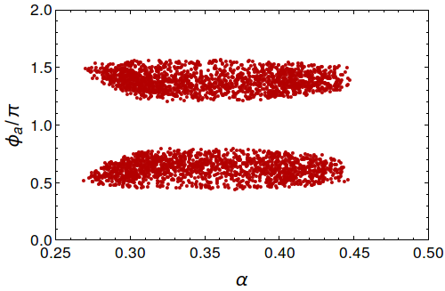
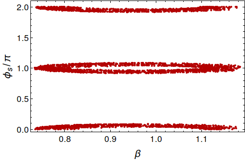
Figure 1: Allowed regions of α𝛼\alpha-ϕasubscriptitalic-ϕ𝑎\phi_{a} (left panel) and β𝛽\beta-ϕssubscriptitalic-ϕ𝑠\phi_{s} (right panel) planes for 3σ𝜎\sigma allowed ranges of θ13subscript𝜃13\theta_{13}, θ12subscript𝜃12\theta_{12}, θ23subscript𝜃23\theta_{23} and the ratio (r𝑟r) of solar to atmospheric mass squared differences Esteban et al. (2017); nuf .

and we obtain

sinθ13eiδ=13(cosθ+sinθeiψ).subscript𝜃13superscript𝑒𝑖𝛿13𝜃𝜃superscript𝑒𝑖𝜓\displaystyle\sin\theta_{13}e^{-i\delta}=\frac{1}{\sqrt{3}}(\cos\theta+\sin\theta e^{-i\psi}). (104)

Now, sinθ13subscript𝜃13\sin\theta_{13} and δ𝛿\delta can also be parametrised in terms of θ𝜃\theta and ψ𝜓\psi as

sin2θ13=13(1+sin2θcosψ)andtanδ=sinθsinψcosθ+sinθcosψ.superscript2subscript𝜃131312𝜃𝜓and𝛿𝜃𝜓𝜃𝜃𝜓\displaystyle\sin^{2}\theta_{13}=\frac{1}{3}(1+\sin 2\theta\cos\psi)~{}~{}{\rm and}~{}~{}\tan\delta=\frac{\sin\theta\sin\psi}{\cos\theta+\sin\theta\cos\psi}. (105)

Such correlation between the model parameters and neutrino mixing angles θ13,θ12,θ23subscript𝜃13subscript𝜃12subscript𝜃23\theta_{13},\theta_{12},\theta_{23}, Dirac CP phase δ𝛿\delta can also be found in Memenga et al. (2013); Grimus and Lavoura (2008); Albright and Rodejohann (2009); Albright et al. (2010); He and Zee (2011); Borah and Karmakar (2018). Therefore from Eq. (102) and Eq. (105) it is clear that the neutrino mixing angles are functions of four model parameters namely, α𝛼\alpha, β𝛽\beta, ϕssubscriptitalic-ϕ𝑠\phi_{s} and ϕasubscriptitalic-ϕ𝑎\phi_{a}. These are the parameters associated with symmetric and anti-symmetric part of the effective light neutrino mass matrix and corresponding relative phases. These parameters then can be constrained using the current data on neutrino mixing angles Esteban et al. (2017); de Salas et al. (2017); nuf . In addition to the bounds obtained from the mixing angles, the parameter space can be further constrained in oder to satisfy correct value for mass squared differences. Here one can define a ratio for the solar to atmospheric mass squared difference as

r=Δm2|ΔmA2|=Δm212|Δm322|.𝑟Δsuperscriptsubscript𝑚direct-product2Δsuperscriptsubscript𝑚𝐴2Δsuperscriptsubscript𝑚212Δsubscriptsuperscript𝑚232\displaystyle r=\frac{\Delta{m}_{\odot}^{2}}{|\Delta{m}_{A}^{2}|}=\frac{\Delta{m_{21}^{2}}}{|\Delta{m}^{2}_{32}|}. (106)
Refer to caption      Refer to caption
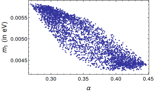
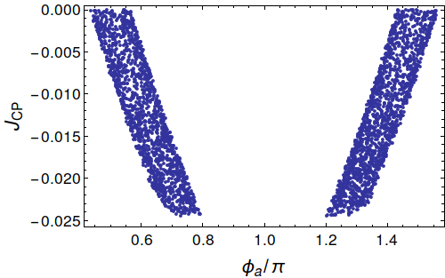
Figure 2: Predictions for lightest neutrino mass m1subscript𝑚1m_{1} as a function of α𝛼\alpha (left panel) and Jarlskog invariant JCPsubscript𝐽𝐶𝑃J_{CP} as a function of ϕasubscriptitalic-ϕ𝑎\phi_{a} (right panel). Here each points in both panels also satisfy 3σ𝜎\sigma allowed ranges for θ13subscript𝜃13\theta_{13}, θ12subscript𝜃12\theta_{12}, θ23subscript𝜃23\theta_{23} and the ratio (r𝑟r) of solar to atmospheric mass squared differences Esteban et al. (2017); nuf .

From Eq. (98)-(100), it is evident that this ratio r𝑟r is a function of the model parameters α𝛼\alpha, β𝛽\beta, ϕssubscriptitalic-ϕ𝑠\phi_{s} and ϕasubscriptitalic-ϕ𝑎\phi_{a}. In order to satisfy correct neutrino oscillation data, we use the 3σ𝜎\sigma allowed range of the neutrino mixing angles and mass squared differences given in global fit analysis Esteban et al. (2017); nuf to constrain these model parameters. Here in Fig. 1 we have shown the allowed regions for parameters α𝛼\alpha, β𝛽\beta, ϕssubscriptitalic-ϕ𝑠\phi_{s} and ϕasubscriptitalic-ϕ𝑎\phi_{a} satisfying 3σ𝜎\sigma ranges for neutrino mixing angles (θ13,θ12,θ23subscript𝜃13subscript𝜃12subscript𝜃23\theta_{13},\theta_{12},\theta_{23}) and ratio of the mass squared differences r𝑟r. In the left panel of Fig. 1 we show the allowed points in α𝛼\alpha-ϕasubscriptitalic-ϕ𝑎\phi_{a} plane whereas in the right panel we have plotted the same in β𝛽\beta-ϕssubscriptitalic-ϕ𝑠\phi_{s} plane. Here we find that the parameter β𝛽\beta, associated with the symmetric part of the neutrino mass matrix ranges between 0.7-1.2 whereas the anti-symmetric part (contained in parameter α𝛼\alpha) remains confined within a relatively narrower region between 0.27 to 0.45. The associated phases also occupy distinct allowed regions as evident from both panels of Fig. 1. After finding the allowed regions for α𝛼\alpha, β𝛽\beta, ϕssubscriptitalic-ϕ𝑠\phi_{s} and ϕasubscriptitalic-ϕ𝑎\phi_{a}, one can easily find out the common factor κ𝜅\kappa appearing in the light neutrino mass eigenvalues using Eq. (98)-(99) and best fit value of solar mass squared difference, Δm212=m22m12=7.40×10⁵Δsuperscriptsubscript𝑚212subscriptsuperscript𝑚22subscriptsuperscript𝑚217.40superscript105\Delta{m_{21}^{2}}=m^{2}_{2}-m^{2}_{1}=7.40\times 10^{-5} eV2 Esteban et al. (2017); nuf . The estimation of κ𝜅\kappa then enables us to find predictions for absolute neutrino masses. In the left panel of Fig. 2, we plot the predictions for lightest absolute neutrino mass m1subscript𝑚1m_{1} as a function of α𝛼\alpha and it ranges between (0.42×1020.42superscript1020.42\times 10^{-2} -0.58×1020.58superscript1020.58\times 10^{-2}) eV for α𝛼\alpha in the range 0.27 to 0.45. Similarly, one can also find the estimates for sum of all three absolute neutrino in this simplified scenario of the neutrino mass matrix and is given by mi=(0.0620.070)subscript𝑚𝑖0.0620.070\sum m_{i}=(0.062-0.070) eV, lying within the cosmological bound on sum of light neutrino masses mi0.17subscript𝑚𝑖0.17\sum m_{i}\leq 0.17 eV from Planck data Ade et al. (2016). On the other hand, in the right panel of Fig. 2, we have plotted the allowed regions for the Jarlskog CP invariant JCP=Im[Ue1Uμ2Ue2Uμ1]subscript𝐽CPImdelimited-[]subscript𝑈𝑒1subscript𝑈𝜇2subscriptsuperscript𝑈𝑒2subscriptsuperscript𝑈𝜇1J_{\rm CP}={\rm Im}[U_{e1}U_{\mu 2}U^{*}_{e2}U^{*}_{\mu 1}] Jarlskog (1985) as a function of the relative phase ϕasubscriptitalic-ϕ𝑎\phi_{a} associated with the anti-symmetric contribution of the neutrino mass matrix and estimated to be within the range |JCP|00.024similar-tosubscript𝐽𝐶𝑃00.024|J_{CP}|\sim 0-0.024.

Refer to caption
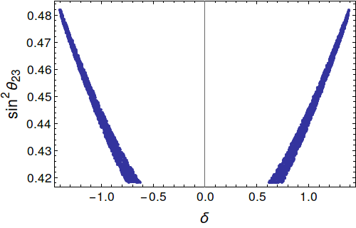
Figure 3: Predicted correlation between Dirac CP phase δ𝛿\delta and atmospheric mixing angle θ23subscript𝜃23\theta_{23} for Case A.

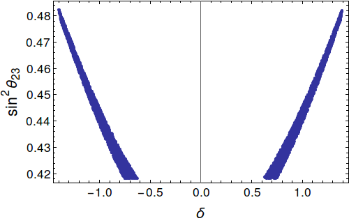
In Fig. 3, we show the most important among such correlations namely, the one between the Dirac CP phase δ𝛿\delta and atmospheric mixing angle θ23subscript𝜃23\theta_{23}. Interestingly, here we find that, the model predicts the CP phase δ𝛿\delta to be in the range π/2δπ/5less-than-or-similar-to𝜋2𝛿less-than-or-similar-to𝜋5-\pi/2\lesssim\delta\lesssim-\pi/5 and π/5δπ/2less-than-or-similar-to𝜋5𝛿less-than-or-similar-to𝜋2\pi/5\lesssim\delta\lesssim\pi/2 whereas sin2θ23superscript2subscript𝜃23\sin^{2}\theta_{23} lies in the lower octant. This value of δ𝛿\delta falls in the current preferred ballpark suggested by experiments Abe et al. (2017) as well as global fit analysis Esteban et al. (2017); nuf , predicting atmospheric mixing angle θ23subscript𝜃23\theta_{23} to be in the lower octant.

II.2 Case B:

In this subsection, we analyse the effective light neutrino mass matrix given in Eq. (52) in a more general canvas to illustrate the effects of contributions coming from symmetric and anti-symmetric parts appearing in the two different terms of the linear seesaw formula, without assuming any equality between two symmetric (and anti-symmetric) terms. Considering the most general structure for the light neutrino mass matrix as given in Eq. (52), we can define a Hermitian matrix as,

\displaystyle\mathcal{M} =mνmνabsentsubscript𝑚𝜈superscriptsubscript𝑚𝜈\displaystyle=m_{\nu}m_{\nu}^{\dagger} (107)
=|λ|2(X10X20X30X40X5)absentsuperscript𝜆2subscript𝑋10subscript𝑋20subscript𝑋30subscript𝑋40subscript𝑋5\displaystyle=|\lambda|^{2}\left(\begin{array}[]{ccc}X_{1}&0&X_{2}\\ 0&X_{3}&0\\ X_{4}&0&X_{5}\end{array}\right) (111)

where

X1subscript𝑋1\displaystyle X_{1} =4|x|2+|(a1+a2)+(s1+s2)|2,absent4superscript𝑥2superscriptsubscript𝑎1subscript𝑎2subscript𝑠1subscript𝑠22\displaystyle=4|x|^{2}+|(a_{1}+a_{2})+(s_{1}+s_{2})|^{2},
X2subscript𝑋2\displaystyle X_{2} =2x{(a1+a2)(s1+s2)}2x{(a1+a2)+(s1+s2)},absent2𝑥superscriptsubscript𝑎1subscript𝑎2superscriptsubscript𝑠1subscript𝑠22superscript𝑥subscript𝑎1subscript𝑎2subscript𝑠1subscript𝑠2\displaystyle=2x\{(a_{1}+a_{2})^{*}-(s_{1}+s_{2})^{*}\}-2x^{*}\{(a_{1}+a_{2})+(s_{1}+s_{2})\},
X3subscript𝑋3\displaystyle X_{3} =1|x|2|(a12+a22)(s12+s22)+2x2|2,absent1superscript𝑥2superscriptsuperscriptsubscript𝑎12superscriptsubscript𝑎22superscriptsubscript𝑠12superscriptsubscript𝑠222superscript𝑥22\displaystyle=\frac{1}{|x|^{2}}|(a_{1}^{2}+a_{2}^{2})-(s_{1}^{2}+s_{2}^{2})+2x^{2}|^{2},
X4subscript𝑋4\displaystyle X_{4} =2x{(a1+a2)(s1+s2)}2x{(a1+a2)+(s1+s2)},absent2superscript𝑥subscript𝑎1subscript𝑎2subscript𝑠1subscript𝑠22𝑥superscriptsubscript𝑎1subscript𝑎2superscriptsubscript𝑠1subscript𝑠2\displaystyle=2x^{*}\{(a_{1}+a_{2})-(s_{1}+s_{2})\}-2x\{(a_{1}+a_{2})^{*}+(s_{1}+s_{2})^{*}\},
X5subscript𝑋5\displaystyle X_{5} =4|x|2+|(a1+a2)(s1+s2)|2.absent4superscript𝑥2superscriptsubscript𝑎1subscript𝑎2subscript𝑠1subscript𝑠22\displaystyle=4|x|^{2}+|(a_{1}+a_{2})-(s_{1}+s_{2})|^{2}.

Here for simplicity, we have considered x1=x2=xsubscript𝑥1subscript𝑥2𝑥x_{1}=x_{2}=x and λ1=λ2=λsubscript𝜆1subscript𝜆2𝜆\lambda_{1}=\lambda_{2}=\lambda while keeping the other terms distinct. This Hermitian matrix \mathcal{M} now can also be diagonalised by a similar rotation matrix (in the 13 plane) given in Eq. (66) with rotation angle θ𝜃\theta and phase factor ψ𝜓\psi. These parameters can therefore be expressed as

tan2θ2𝜃\displaystyle\tan 2\theta =\displaystyle= 2[AsinψBcosψ]C1+C2+C3+C4,tanψ=AB,2delimited-[]𝐴𝜓𝐵𝜓subscript𝐶1subscript𝐶2subscript𝐶3subscript𝐶4𝜓𝐴𝐵\displaystyle\frac{2\left[A\sin\psi-B\cos\psi\right]}{C_{1}+C_{2}+C_{3}+C_{4}},~{}~{}~{}\tan\psi=-\frac{A}{B}, (112)

with

A𝐴\displaystyle A =\displaystyle= (α1sinϕa1+α2sinϕa2),B=(β1cosϕs1+β2cosϕs2),subscript𝛼1subscriptitalic-ϕsubscript𝑎1subscript𝛼2subscriptitalic-ϕsubscript𝑎2𝐵subscript𝛽1subscriptitalic-ϕsubscript𝑠1subscript𝛽2subscriptitalic-ϕsubscript𝑠2\displaystyle(\alpha_{1}\sin\phi_{a_{1}}+\alpha_{2}\sin\phi_{a_{2}}),~{}~{}~{}B=(\beta_{1}\cos\phi_{s_{1}}+\beta_{2}\cos\phi_{s_{2}}), (113)
C1subscript𝐶1\displaystyle C_{1} =\displaystyle= α1β1cos(ϕa1ϕs1),C2=α1β2cos(ϕa1ϕs2),subscript𝛼1subscript𝛽1subscriptitalic-ϕsubscript𝑎1subscriptitalic-ϕsubscript𝑠1subscript𝐶2subscript𝛼1subscript𝛽2subscriptitalic-ϕsubscript𝑎1subscriptitalic-ϕsubscript𝑠2\displaystyle\alpha_{1}\beta_{1}\cos(\phi_{a_{1}}-\phi_{s_{1}}),~{}~{}~{}~{}C_{2}=\alpha_{1}\beta_{2}\cos(\phi_{a_{1}}-\phi_{s_{2}}), (114)
C3subscript𝐶3\displaystyle C_{3} =\displaystyle= α2β1cos(ϕa2ϕs1),C4=α2β2cos(ϕa2ϕs2),subscript𝛼2subscript𝛽1subscriptitalic-ϕsubscript𝑎2subscriptitalic-ϕsubscript𝑠1subscript𝐶4subscript𝛼2subscript𝛽2subscriptitalic-ϕsubscript𝑎2subscriptitalic-ϕsubscript𝑠2\displaystyle\alpha_{2}\beta_{1}\cos(\phi_{a_{2}}-\phi_{s_{1}}),~{}~{}~{}~{}C_{4}=\alpha_{2}\beta_{2}\cos(\phi_{a_{2}}-\phi_{s_{2}}), (115)

where we have defined the parameters as αj=|aj|/|x|subscript𝛼𝑗subscript𝑎𝑗𝑥\alpha_{j}=|a_{j}|/|x|, βj=|sj|/|x|subscript𝛽𝑗subscript𝑠𝑗𝑥\beta_{j}=|s_{j}|/|x|, ϕajx=ϕajϕxsubscriptitalic-ϕsubscript𝑎𝑗𝑥subscriptitalic-ϕsubscript𝑎𝑗subscriptitalic-ϕ𝑥\phi_{a_{j}x}=\phi_{a_{j}}-\phi_{x}, ϕsjx=ϕsjϕxsubscriptitalic-ϕsubscript𝑠𝑗𝑥subscriptitalic-ϕsubscript𝑠𝑗subscriptitalic-ϕ𝑥\phi_{s_{j}x}=\phi_{s_{j}}-\phi_{x}, sj=|s|ejϕsjsubscript𝑠𝑗𝑠superscript𝑒𝑗subscriptitalic-ϕsubscript𝑠𝑗s_{j}=|s|e^{j\phi_{s_{j}}}, aj=|a|eiϕajsubscript𝑎𝑗𝑎superscript𝑒𝑖subscriptitalic-ϕsubscript𝑎𝑗a_{j}=|a|e^{i\phi_{a_{j}}} and x=|x|eiϕx𝑥𝑥superscript𝑒𝑖subscriptitalic-ϕ𝑥x=|x|e^{i\phi_{x}} with j=1,2𝑗12j=1,2. For notational compactness we have written the relative phases ϕajx,ϕsjxsubscriptitalic-ϕsubscript𝑎𝑗𝑥subscriptitalic-ϕsubscript𝑠𝑗𝑥\phi_{a_{j}x},\phi_{s_{j}x} in equation (113-115) as ϕaj,ϕsjsubscriptitalic-ϕsubscript𝑎𝑗subscriptitalic-ϕsubscript𝑠𝑗\phi_{a_{j}},\phi_{s_{j}} with j=1,2𝑗12j=1,2. Hence, diagonalising the Hermitian matrix via U13U13=diag(m12,m22,m32)superscriptsubscript𝑈13subscript𝑈13diagsuperscriptsubscript𝑚12superscriptsubscript𝑚22superscriptsubscript𝑚32U_{13}^{\dagger}\mathcal{M}U_{13}={\rm diag}(m_{1}^{2},m_{2}^{2},m_{3}^{2}), we obtain the light neutrino masses as

m12superscriptsubscript𝑚12\displaystyle m_{1}^{2} =\displaystyle= κ2[4+α12+α22+β12+β22+C54(C1+C2+C3+C4)2+42(A2+B2)],superscript𝜅2delimited-[]4superscriptsubscript𝛼12superscriptsubscript𝛼22superscriptsubscript𝛽12superscriptsubscript𝛽22subscript𝐶54superscriptsubscript𝐶1subscript𝐶2subscript𝐶3subscript𝐶42superscript42superscript𝐴2superscript𝐵2\displaystyle\kappa^{2}\left[4+\alpha_{1}^{2}+\alpha_{2}^{2}+\beta_{1}^{2}+\beta_{2}^{2}+C_{5}-\sqrt{4(C_{1}+C_{2}+C_{3}+C_{4})^{2}+4^{2}(A^{2}+B^{2})}\right], (116)
m22superscriptsubscript𝑚22\displaystyle m_{2}^{2} =\displaystyle= κ2[4+α14+α24+β14+β24+C6],superscript𝜅2delimited-[]4superscriptsubscript𝛼14superscriptsubscript𝛼24superscriptsubscript𝛽14superscriptsubscript𝛽24subscript𝐶6\displaystyle\kappa^{2}\left[4+\alpha_{1}^{4}+\alpha_{2}^{4}+\beta_{1}^{4}+\beta_{2}^{4}+C_{6}\right], (117)
m32superscriptsubscript𝑚32\displaystyle m_{3}^{2} =\displaystyle= κ2[4+α12+α22+β12+β22+C5+4(C1+C2+C3+C4)2+42(A2+B2)],superscript𝜅2delimited-[]4superscriptsubscript𝛼12superscriptsubscript𝛼22superscriptsubscript𝛽12superscriptsubscript𝛽22subscript𝐶54superscriptsubscript𝐶1subscript𝐶2subscript𝐶3subscript𝐶42superscript42superscript𝐴2superscript𝐵2\displaystyle\kappa^{2}\left[4+\alpha_{1}^{2}+\alpha_{2}^{2}+\beta_{1}^{2}+\beta_{2}^{2}+C_{5}+\sqrt{4(C_{1}+C_{2}+C_{3}+C_{4})^{2}+4^{2}(A^{2}+B^{2})}\right], (118)

where

C5subscript𝐶5\displaystyle C_{5} =\displaystyle= 2{α1α2cos(ϕa1ϕa2)+β1β2cos(ϕs1ϕs2)},2subscript𝛼1subscript𝛼2subscriptitalic-ϕsubscript𝑎1subscriptitalic-ϕsubscript𝑎2subscript𝛽1subscript𝛽2subscriptitalic-ϕsubscript𝑠1subscriptitalic-ϕsubscript𝑠2\displaystyle 2\{\alpha_{1}\alpha_{2}\cos(\phi_{a_{1}}-\phi_{a_{2}})+\beta_{1}\beta_{2}\cos(\phi_{s_{1}}-\phi_{s_{2}})\},
C6subscript𝐶6\displaystyle C_{6} =\displaystyle= 4(α12cos2ϕa1+α22cos2ϕa2)4(β12cos2ϕs1+β22cos2ϕs2)4superscriptsubscript𝛼122subscriptitalic-ϕsubscript𝑎1superscriptsubscript𝛼222subscriptitalic-ϕsubscript𝑎24superscriptsubscript𝛽122subscriptitalic-ϕsubscript𝑠1superscriptsubscript𝛽222subscriptitalic-ϕsubscript𝑠2\displaystyle 4(\alpha_{1}^{2}\cos 2\phi_{a_{1}}+\alpha_{2}^{2}\cos 2\phi_{a_{2}})-4(\beta_{1}^{2}\cos 2\phi_{s_{1}}+\beta_{2}^{2}\cos 2\phi_{s_{2}})
+2α12α22cos2(ϕa1ϕa2)2α12β12cos2(ϕa1ϕs1)2α12β22cos2(ϕa1ϕs2)2superscriptsubscript𝛼12superscriptsubscript𝛼222subscriptitalic-ϕsubscript𝑎1subscriptitalic-ϕsubscript𝑎22superscriptsubscript𝛼12superscriptsubscript𝛽122subscriptitalic-ϕsubscript𝑎1subscriptitalic-ϕsubscript𝑠12superscriptsubscript𝛼12superscriptsubscript𝛽222subscriptitalic-ϕsubscript𝑎1subscriptitalic-ϕsubscript𝑠2\displaystyle+2\alpha_{1}^{2}\alpha_{2}^{2}\cos 2(\phi_{a_{1}}-\phi_{a_{2}})-2\alpha_{1}^{2}\beta_{1}^{2}\cos 2(\phi_{a_{1}}-\phi_{s_{1}})-2\alpha_{1}^{2}\beta_{2}^{2}\cos 2(\phi_{a_{1}}-\phi_{s_{2}})
2α22β12cos2(ϕa2ϕs1)2α22β22cos2(ϕa1ϕs2)+2β12β22cos2(ϕs1ϕs2).2superscriptsubscript𝛼22superscriptsubscript𝛽122subscriptitalic-ϕsubscript𝑎2subscriptitalic-ϕsubscript𝑠12superscriptsubscript𝛼22superscriptsubscript𝛽222subscriptitalic-ϕsubscript𝑎1subscriptitalic-ϕsubscript𝑠22superscriptsubscript𝛽12superscriptsubscript𝛽222subscriptitalic-ϕsubscript𝑠1subscriptitalic-ϕsubscript𝑠2\displaystyle-2\alpha_{2}^{2}\beta_{1}^{2}\cos 2(\phi_{a_{2}}-\phi_{s_{1}})-2\alpha_{2}^{2}\beta_{2}^{2}\cos 2(\phi_{a_{1}}-\phi_{s_{2}})+2\beta_{1}^{2}\beta_{2}^{2}\cos 2(\phi_{s_{1}}-\phi_{s_{2}}).

Considering the contributions from both charged lepton and neutrino sectors, the complete lepton mixing matrix in this general case also is given by

U𝑈\displaystyle U =\displaystyle= UωU13.subscriptsuperscript𝑈𝜔subscript𝑈13\displaystyle U^{\dagger}_{\omega}U_{13}. (119)
Refer to captionRefer to caption
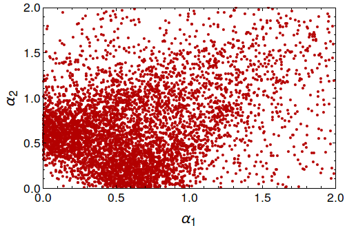
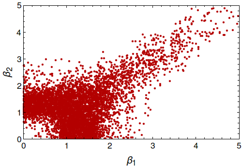
Figure 4: Allowed regions of α1subscript𝛼1\alpha_{1}-α2subscript𝛼2\alpha_{2} (left panel) and β1subscript𝛽1\beta_{1}-β2subscript𝛽2\beta_{2} (right panel) planes for 3σ𝜎\sigma allowed ranges of θ13subscript𝜃13\theta_{13}, θ12subscript𝜃12\theta_{12}, θ23subscript𝜃23\theta_{23} and the ratio (r𝑟r) of solar to atmospheric mass squared differences Esteban et al. (2017); nuf . These points additionally also satisfy the upper limit for sum of the three absolute neutrino masses mi0.17subscript𝑚𝑖0.17\sum m_{i}\leq 0.17 eV Abe et al. (2017).
Refer to captionRefer to caption
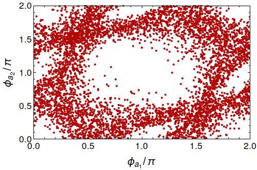
Figure 5: Allowed regions of ϕa1subscriptitalic-ϕsubscript𝑎1\phi_{a_{1}}-ϕa2subscriptitalic-ϕsubscript𝑎2\phi_{a_{2}} (left panel) and ϕb1subscriptitalic-ϕsubscript𝑏1\phi_{b_{1}}-ϕb2subscriptitalic-ϕsubscript𝑏2\phi_{b_{2}} (right panel) planes for 3σ𝜎\sigma allowed ranges of θ13subscript𝜃13\theta_{13}, θ12subscript𝜃12\theta_{12}, θ23subscript𝜃23\theta_{23} and the ratio (r𝑟r) of solar to atmospheric mass squared differences Esteban et al. (2017); nuf . These points additionally also satisfy the upper limit for sum of the three absolute neutrino mass mi0.17subscript𝑚𝑖0.17\sum m_{i}\leq 0.17 eV Abe et al. (2017).

Comparing this mixing matrix with UPMNSsubscript𝑈PMNSU_{\rm PMNS} as given in Eq. (103), one can obtain the correlations between the the mixing angles (θ13subscript𝜃13\theta_{13}, θ12subscript𝜃12\theta_{12} and θ23subscript𝜃23\theta_{23}) and Dirac CP phase δ𝛿\delta as previously given in Eq. (105). Further using Eq. (112) we find the correspondence between neutrino mixing angles and the relevant model parameters. Here the parameters αj,βj,ϕajsubscript𝛼𝑗subscript𝛽𝑗subscriptitalic-ϕsubscript𝑎𝑗\alpha_{j},\beta_{j},\phi_{a_{j}} and ϕsjsubscriptitalic-ϕsubscript𝑠𝑗\phi_{s_{j}} with j=1,2𝑗12j=1,2 essentially dictate the neutrino mixing patterns. Obviously, the number of parameters controlling neutrino mixing in this general case is more than what it was in the simple scenario described earlier.
Refer to captionRefer to caption
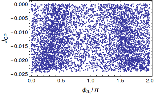
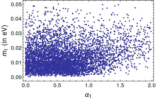
Figure 6: Predictions for lightest neutrino mass m1subscript𝑚1m_{1} as a function of α1subscript𝛼1\alpha_{1} (left panel) and Jarlskog invariant JCPsubscript𝐽CPJ_{\rm CP} as a function of ϕa1subscriptitalic-ϕsubscript𝑎1\phi_{a_{1}} (right panel). Here each points in both panels also satisfy 3σ𝜎\sigma allowed values of θ13subscript𝜃13\theta_{13}, θ12subscript𝜃12\theta_{12}, θ23subscript𝜃23\theta_{23} and the ratio (r𝑟r) of solar to atmospheric mass squared differences Esteban et al. (2017); nuf .

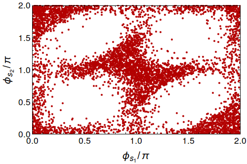
Using Eq. (116)-(118) we define a ratio r(=Δm2/|ΔmA2|=Δm212/|Δm322|)r(=\Delta{m}_{\odot}^{2}/|\Delta{m}_{A}^{2}|=\Delta{m_{21}^{2}}/|\Delta{m}^{2}_{32}|) in terms of very same parameters αj,βj,ϕajsubscript𝛼𝑗subscript𝛽𝑗subscriptitalic-ϕsubscript𝑎𝑗\alpha_{j},\beta_{j},\phi_{a_{j}} and ϕsjsubscriptitalic-ϕsubscript𝑠𝑗\phi_{s_{j}}. Here also to satisfy correct neutrino oscillation data, we use the 3σ𝜎\sigma range of the neutrino mixing angle and mass squared differences Esteban et al. (2017); nuf to constrain these parameters and we find the correlations among them. In addition to the bounds from neutrino oscillation experiments, these parameters can also get constrained in order to satisfy the cosmological upper limit on sum of the three absolute neutrino mass, given by mi0.17subscript𝑚𝑖0.17\sum m_{i}\leq 0.17 eV Abe et al. (2017). Therefore, using all these constraints, in Fig. 4 we have all the allowed points in α1subscript𝛼1\alpha_{1}-α2subscript𝛼2\alpha_{2} (left panel) plane and β1subscript𝛽1\beta_{1}-β2subscript𝛽2\beta_{2} (right panel) plane respectively. In the left panel, we find that the contributions involving the anti-symmetric parts (α1subscript𝛼1\alpha_{1} and α2subscript𝛼2\alpha_{2}) are mostly confined within 0-2. On the other hand, as it is evident from the right panel of Fig. 4, the contributions involving the symmetric parts (β1subscript𝛽1\beta_{1} and β2subscript𝛽2\beta_{2}) take relatively larger values satisfying correct neutrino oscillation data. Then in Fig. 5, we show the allowed parameter space in the ϕa1subscriptitalic-ϕsubscript𝑎1\phi_{a_{1}}-ϕa2subscriptitalic-ϕsubscript𝑎2\phi_{a_{2}} plane (left panel) and ϕb1subscriptitalic-ϕsubscript𝑏1\phi_{b_{1}}-ϕb2subscriptitalic-ϕsubscript𝑏2\phi_{b_{2}} plane (right panel) respectively which clearly show distinct correlations between relative phases associated with symmetric and anti-symmetric contributions.
Refer to caption
Figure 7: Predicted correlation between Dirac CP phase δ𝛿\delta and atmospheric mixing angle θ23subscript𝜃23\theta_{23} for Case B.

After finding the allowed regions for α1,2subscript𝛼12\alpha_{1,2}, β1,2subscript𝛽12\beta_{1,2}, ϕa1,2subscriptitalic-ϕsubscript𝑎12\phi_{a_{1,2}} and ϕs1,2subscriptitalic-ϕsubscript𝑠12\phi_{s_{1,2}}, one can again find out the common factor κ𝜅\kappa appearing in the light neutrino mass eigenvalues involved in this general case using Eq. (116)-(117) and best fit value of solar mass squared difference, Δm212=m22m12=7.40×10⁵Δsuperscriptsubscript𝑚212subscriptsuperscript𝑚22subscriptsuperscript𝑚217.40superscript105\Delta{m_{21}^{2}}=m^{2}_{2}-m^{2}_{1}=7.40\times 10^{-5} eV2 Esteban et al. (2017); nuf as mentioned earlier. The estimate for κ𝜅\kappa enables us to find predictions for absolute neutrino masses using Eq. (116)-(117). In the left panel of Fig. 6, we show the predictions for lightest absolute neutrino mass m1subscript𝑚1m_{1} as a function of α1subscript𝛼1\alpha_{1} (parameter involved in one of the anti-symmetric contribution). It can be seen from this plot that m1subscript𝑚1m_{1} can be as large as 0.050.050.05 eV for α1subscript𝛼1\alpha_{1} within the limit of 2. Such values of the lightest neutrino mass correspond to sum of all three absolute neutrino masses mi=(0.060.17)subscript𝑚𝑖0.060.17\sum m_{i}=(0.06-0.17) eV saturating the cosmological upper limit. In the right panel of Fig. 6, we have again plotted the allowed regions for the Jarlskog CP invariant JCPsubscript𝐽CPJ_{\rm CP} as a function of the relative phase ϕa1subscriptitalic-ϕsubscript𝑎1\phi_{a_{1}} associated with one of the anti-symmetric contribution of the neutrino mass matrix and estimated to be within the range |JCP|00.024similar-tosubscript𝐽CP00.024|J_{\rm CP}|\sim 0-0.024, analogous to the previous result. In Fig. 7, we have now plotted the correlation between the Dirac CP phase δ𝛿\delta and atmospheric mixing angle θ23subscript𝜃23\theta_{23}. Similar to the previous case, here also we find that, the model predicts the Dirac CP phase δ𝛿\delta to be in the range π/2δπ/5less-than-or-similar-to𝜋2𝛿less-than-or-similar-to𝜋5-\pi/2\lesssim\delta\lesssim-\pi/5 and π/5δπ/2less-than-or-similar-to𝜋5𝛿less-than-or-similar-to𝜋2\pi/5\lesssim\delta\lesssim\pi/2 whereas θ23subscript𝜃23\theta_{23} lies in the lower octant.

In this two different limits of Dirac linear seesaw discussed above, we have observed that the allowed range of the light neutrino mass is different in the two cases. In Case A, due to much constrained scenario of the neutrino mass matrix
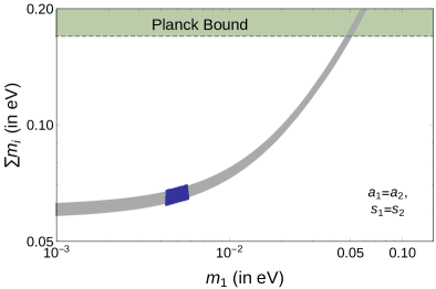
Refer to caption      Refer to caption
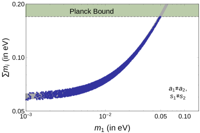
Figure 8: Comparison for misubscript𝑚𝑖\sum m_{i} as a function of lightest neutrino mass m1subscript𝑚1m_{1} in both cases A and B.

the correlation between m1subscript𝑚1m_{1} and misubscript𝑚𝑖\sum m_{i} is mainly concentrated within a narrow region. This is shown in the left panel of Fig. 8. However, for the Case B, due to presence of more number of parameters originated from both the contributions of linear seesaw formula being distinct, the constrains are much more relaxed. In this case neutrino masses can vary from a very small values to larger ones saturating the cosmological upper bound mi0.17subscript𝑚𝑖0.17\sum m_{i}\leq 0.17 eV. Here the whole region is basically allowed, as shown in the right panel of Fig. 8. Finally, it is important to mention that, within these two different limits, inverted hierarchy of neutrino mass is not allowed, another important prediction of our model.

III Conclusion

We have proposed a linear seesaw model for Dirac neutrinos in this work. After proposing a renormalisable version of such seesaw by extending the SM with appropriate fields and global symmetries, we move on to a more predictive framework of A4subscript𝐴4A_{4} flavour symmetry. While in the renormalisable version, the seesaw scale can be brought down to the TeV scale by assuming smallness of certain terms in the seesaw mass matrix, which can be justified by incorporating additional approximate global symmetries. In the A4subscript𝐴4A_{4} symmetric version additional discrete and global lepton number symmetry are chosen in a manner to make sure that the correct hierarchy between different terms appearing in the complete neutral fermion mass matrix is naturally obtained without making any assumptions or referring to approximate global symmetries. The interesting feature of the conventional linear seesaw framework where a small lepton number breaking term in seesaw formula, linear in Dirac neutrino mass, can give rise to correct neutrino mass with heavy neutrinos lying in TeV scale, is retained in the Dirac version of it by appropriately generating hierarchical terms at different orders (dimension four and dimension five). Since lepton number is present as a global unbroken symmetry in the model, all the mass matrices involved are of Dirac type and hence the A4subscript𝐴4A_{4} triple products contain the anti-symmetric components which play a crucial role in generating the correct neutrino phenomenology. Since we use the S𝑆S diagonal basis of A4subscript𝐴4A_{4} for Dirac neutrino case, the charged lepton mass matrix is also non trivial in our scenarios and hence can contribute to the leptonic mixing matrix. For generic choices of A4subscript𝐴4A_{4} flavon alignments, we find that the model remains very predictive in terms of neutrino mass hierarchy, leptonic CP phase, octant of atmospheric mixing angle as well as absolute neutrino masses. While the neutrino mass hierarchy is predicted to be the normal one, the Dirac CP phase δ𝛿\delta is found to lie in the range π/2δπ/5less-than-or-similar-to𝜋2𝛿less-than-or-similar-to𝜋5-\pi/2\lesssim\delta\lesssim-\pi/5 and π/5δπ/2less-than-or-similar-to𝜋5𝛿less-than-or-similar-to𝜋2\pi/5\lesssim\delta\lesssim\pi/2 whereas the atmospheric mixing angle θ23subscript𝜃23\theta_{23} lies in the lower octant. The predictions for lightest neutrino mass, in one of the scenarios, can saturate the cosmological upper bound on the sum of absolute neutrino masses mi0.17subscript𝑚𝑖0.17\sum m_{i}\leq 0.17 eV. Apart from these, being a model predicting Dirac neutrinos, it can also predict the absence of lepton number violation and hence can not be tested in ongoing and future neutrinoless double beta decay experiments. These aspects keep the detection prospects of the model very promising at experiments ranging from neutrino oscillations, cosmology to rare decay ones.

Acknowledgements.
One of the authors, DB acknowledges the hospitality and facilities provided by Seoul-Tech, Korea and KEK Theory Center, Japan during June, 2018 where part of this work was completed.

Appendix A A4subscript𝐴4A_{4} Multiplication Rules

A4subscript𝐴4A_{4}, the symmetry group of a tetrahedron, is a discrete non-abelian group of even permutations of four objects. It has four irreducible representations: three one-dimensional and one three dimensional which are denoted by 𝟏,𝟏,𝟏′′1superscript1superscript1′′\bf{1},\bf{1^{\prime}},\bf{1^{\prime\prime}} and 𝟑3\bf{3} respectively, being consistent with the sum of square of the dimensions ini2=12subscript𝑖superscriptsubscript𝑛𝑖212\sum_{i}n_{i}^{2}=12. We denote a generic permutation (1,2,3,4)(n1,n2,n3,n4)1234subscript𝑛1subscript𝑛2subscript𝑛3subscript𝑛4(1,2,3,4)\rightarrow(n_{1},n_{2},n_{3},n_{4}) simply by (n1n2n3n4)subscript𝑛1subscript𝑛2subscript𝑛3subscript𝑛4(n_{1}n_{2}n_{3}n_{4}). The group A4subscript𝐴4A_{4} can be generated by two basic permutations S𝑆S and T𝑇T given by S=(4321),T=(2314)formulae-sequence𝑆4321𝑇2314S=(4321),T=(2314). This satisfies

S2=T3=(ST)3=1superscript𝑆2superscript𝑇3superscript𝑆𝑇31S^{2}=T^{3}=(ST)^{3}=1

which is called a presentation of the group. Their product rules of the irreducible representations are given as

𝟏𝟏=𝟏tensor-product111\bf{1}\otimes\bf{1}=\bf{1}
𝟏𝟏=𝟏′′tensor-productsuperscript1superscript1superscript1′′\bf{1^{\prime}}\otimes\bf{1^{\prime}}=\bf{1^{\prime\prime}}
𝟏𝟏′′=𝟏tensor-productsuperscript1superscript1′′1\bf{1^{\prime}}\otimes\bf{1^{\prime\prime}}=\bf{1}
𝟏′′𝟏′′=𝟏tensor-productsuperscript1′′superscript1′′superscript1\bf{1^{\prime\prime}}\otimes\bf{1^{\prime\prime}}=\bf{1^{\prime}}
𝟑𝟑=𝟏𝟏𝟏′′𝟑𝐚𝟑𝐬tensor-product33tensor-product1superscript1superscript1′′subscript3𝐚subscript3𝐬\bf{3}\otimes\bf{3}=\bf{1}\otimes\bf{1^{\prime}}\otimes\bf{1^{\prime\prime}}\otimes\bf{3}_{a}\otimes\bf{3}_{s}

where a𝑎a and s𝑠s in the subscript corresponds to anti-symmetric and symmetric parts respectively. Denoting two triplets as (a1,b1,c1)subscript𝑎1subscript𝑏1subscript𝑐1(a_{1},b_{1},c_{1}) and (a2,b2,c2)subscript𝑎2subscript𝑏2subscript𝑐2(a_{2},b_{2},c_{2}) respectively, their direct product can be decomposed into the direct sum mentioned above. In the S𝑆S diagonal basis, the products are given as

𝟏𝐚𝟏𝐚𝟐+𝐛𝟏𝐛𝟐+𝐜𝟏𝐜𝟐1subscript𝐚1subscript𝐚2subscript𝐛1subscript𝐛2subscript𝐜1subscript𝐜2\bf{1}\backsim a_{1}a_{2}+b_{1}b_{2}+c_{1}c_{2}
𝟏𝐚𝟏𝐚𝟐+ω𝟐𝐛𝟏𝐛𝟐+ω𝐜𝟏𝐜𝟐superscript1subscript𝐚1subscript𝐚2superscript𝜔2subscript𝐛1subscript𝐛2𝜔subscript𝐜1subscript𝐜2\bf{1^{\prime}}\backsim a_{1}a_{2}+\omega^{2}b_{1}b_{2}+\omega c_{1}c_{2}
𝟏′′𝐚𝟏𝐚𝟐+ω𝐛𝟏𝐛𝟐+ω𝟐𝐜𝟏𝐜𝟐superscript1′′subscript𝐚1subscript𝐚2𝜔subscript𝐛1subscript𝐛2superscript𝜔2subscript𝐜1subscript𝐜2\bf{1^{\prime\prime}}\backsim a_{1}a_{2}+\omega b_{1}b_{2}+\omega^{2}c_{1}c_{2}
𝟑𝐬(𝐛𝟏𝐜𝟐+𝐜𝟏𝐛𝟐,𝐜𝟏𝐚𝟐+𝐚𝟏𝐜𝟐,𝐚𝟏𝐛𝟐+𝐛𝟏𝐚𝟐)subscript3𝐬subscript𝐛1subscript𝐜2subscript𝐜1subscript𝐛2subscript𝐜1subscript𝐚2subscript𝐚1subscript𝐜2subscript𝐚1subscript𝐛2subscript𝐛1subscript𝐚2\bf{3}_{s}\backsim(b_{1}c_{2}+c_{1}b_{2},c_{1}a_{2}+a_{1}c_{2},a_{1}b_{2}+b_{1}a_{2})
𝟑𝐚(𝐛𝟏𝐜𝟐𝐜𝟏𝐛𝟐,𝐜𝟏𝐚𝟐𝐚𝟏𝐜𝟐,𝐚𝟏𝐛𝟐𝐛𝟏𝐚𝟐)subscript3𝐚subscript𝐛1subscript𝐜2subscript𝐜1subscript𝐛2subscript𝐜1subscript𝐚2subscript𝐚1subscript𝐜2subscript𝐚1subscript𝐛2subscript𝐛1subscript𝐚2\bf{3}_{a}\backsim(b_{1}c_{2}-c_{1}b_{2},c_{1}a_{2}-a_{1}c_{2},a_{1}b_{2}-b_{1}a_{2})

In the T𝑇T diagonal basis on the other hand, they can be written as

𝟏𝐚𝟏𝐚𝟐+𝐛𝟏𝐜𝟐+𝐜𝟏𝐛𝟐1subscript𝐚1subscript𝐚2subscript𝐛1subscript𝐜2subscript𝐜1subscript𝐛2\bf{1}\backsim a_{1}a_{2}+b_{1}c_{2}+c_{1}b_{2}
𝟏𝐜𝟏𝐜𝟐+𝐚𝟏𝐛𝟐+𝐛𝟏𝐚𝟐superscript1subscript𝐜1subscript𝐜2subscript𝐚1subscript𝐛2subscript𝐛1subscript𝐚2\bf{1^{\prime}}\backsim c_{1}c_{2}+a_{1}b_{2}+b_{1}a_{2}
𝟏′′𝐛𝟏𝐛𝟐+𝐜𝟏𝐚𝟐+𝐚𝟏𝐜𝟐superscript1′′subscript𝐛1subscript𝐛2subscript𝐜1subscript𝐚2subscript𝐚1subscript𝐜2\bf{1^{\prime\prime}}\backsim b_{1}b_{2}+c_{1}a_{2}+a_{1}c_{2}
𝟑𝐬𝟏𝟑(𝟐𝐚𝟏𝐚𝟐𝐛𝟏𝐜𝟐𝐜𝟏𝐛𝟐,𝟐𝐜𝟏𝐜𝟐𝐚𝟏𝐛𝟐𝐛𝟏𝐚𝟐,𝟐𝐛𝟏𝐛𝟐𝐚𝟏𝐜𝟐𝐜𝟏𝐚𝟐)subscript3𝐬132subscript𝐚1subscript𝐚2subscript𝐛1subscript𝐜2subscript𝐜1subscript𝐛22subscript𝐜1subscript𝐜2subscript𝐚1subscript𝐛2subscript𝐛1subscript𝐚22subscript𝐛1subscript𝐛2subscript𝐚1subscript𝐜2subscript𝐜1subscript𝐚2\bf{3}_{s}\backsim\frac{1}{3}(2a_{1}a_{2}-b_{1}c_{2}-c_{1}b_{2},2c_{1}c_{2}-a_{1}b_{2}-b_{1}a_{2},2b_{1}b_{2}-a_{1}c_{2}-c_{1}a_{2})
𝟑𝐚𝟏𝟐(𝐛𝟏𝐜𝟐𝐜𝟏𝐛𝟐,𝐚𝟏𝐛𝟐𝐛𝟏𝐚𝟐,𝐜𝟏𝐚𝟐𝐚𝟏𝐜𝟐)subscript3𝐚12subscript𝐛1subscript𝐜2subscript𝐜1subscript𝐛2subscript𝐚1subscript𝐛2subscript𝐛1subscript𝐚2subscript𝐜1subscript𝐚2subscript𝐚1subscript𝐜2\bf{3}_{a}\backsim\frac{1}{2}(b_{1}c_{2}-c_{1}b_{2},a_{1}b_{2}-b_{1}a_{2},c_{1}a_{2}-a_{1}c_{2})

References

  • Patrignani et al. (2016) C. Patrignani et al. (Particle Data Group), Chin. Phys. C40, 100001 (2016).
  • Esteban et al. (2017) I. Esteban, M. C. Gonzalez-Garcia, M. Maltoni, I. Martinez-Soler, and T. Schwetz, JHEP 01, 087 (2017), eprint 1611.01514.
  • de Salas et al. (2017) P. F. de Salas, D. V. Forero, C. A. Ternes, M. Tortola, and J. W. F. Valle (2017), eprint 1708.01186.
  • (4) Nufit 3.2 (2018), www.nu-fit.org.
  • Gando et al. (2016) A. Gando et al. (KamLAND-Zen), Phys. Rev. Lett. 117, 082503 (2016), [Addendum: Phys. Rev. Lett.117,no.10,109903(2016)], eprint 1605.02889.
  • Minkowski (1977) P. Minkowski, Phys. Lett. B67, 421 (1977).
  • Gell-Mann et al. (1979) M. Gell-Mann, P. Ramond, and R. Slansky, Conf. Proc. C790927, 315 (1979), eprint 1306.4669.
  • Mohapatra and Senjanovic (1980) R. N. Mohapatra and G. Senjanovic, Phys. Rev. Lett. 44, 912 (1980).
  • Schechter and Valle (1980) J. Schechter and J. W. F. Valle, Phys. Rev. D22, 2227 (1980).
  • Babu and He (1989) K. S. Babu and X. G. He, Mod. Phys. Lett. A4, 61 (1989).
  • Peltoniemi et al. (1993) J. T. Peltoniemi, D. Tommasini, and J. W. F. Valle, Phys. Lett. B298, 383 (1993).
  • Centelles Chuliá et al. (2017a) S. Centelles Chuliá, E. Ma, R. Srivastava, and J. W. F. Valle, Phys. Lett. B767, 209 (2017a), eprint 1606.04543.
  • Aranda et al. (2014) A. Aranda, C. Bonilla, S. Morisi, E. Peinado, and J. W. F. Valle, Phys. Rev. D89, 033001 (2014), eprint 1307.3553.
  • Chen et al. (2016) P. Chen, G.-J. Ding, A. D. Rojas, C. A. Vaquera-Araujo, and J. W. F. Valle, JHEP 01, 007 (2016), eprint 1509.06683.
  • Ma et al. (2015) E. Ma, N. Pollard, R. Srivastava, and M. Zakeri, Phys. Lett. B750, 135 (2015), eprint 1507.03943.
  • Reig et al. (2016) M. Reig, J. W. F. Valle, and C. A. Vaquera-Araujo, Phys. Rev. D94, 033012 (2016), eprint 1606.08499.
  • Wang and Han (2016) W. Wang and Z.-L. Han (2016), [JHEP04,166(2017)], eprint 1611.03240.
  • Wang et al. (2017) W. Wang, R. Wang, Z.-L. Han, and J.-Z. Han, Eur. Phys. J. C77, 889 (2017), eprint 1705.00414.
  • Wang et al. (2006) F. Wang, W. Wang, and J. M. Yang, Europhys. Lett. 76, 388 (2006), eprint hep-ph/0601018.
  • Gabriel and Nandi (2007) S. Gabriel and S. Nandi, Phys. Lett. B655, 141 (2007), eprint hep-ph/0610253.
  • Davidson and Logan (2009) S. M. Davidson and H. E. Logan, Phys. Rev. D80, 095008 (2009), eprint 0906.3335.
  • Davidson and Logan (2010) S. M. Davidson and H. E. Logan, Phys. Rev. D82, 115031 (2010), eprint 1009.4413.
  • Bonilla and Valle (2016) C. Bonilla and J. W. F. Valle, Phys. Lett. B762, 162 (2016), eprint 1605.08362.
  • Farzan and Ma (2012) Y. Farzan and E. Ma, Phys. Rev. D86, 033007 (2012), eprint 1204.4890.
  • Bonilla et al. (2016) C. Bonilla, E. Ma, E. Peinado, and J. W. F. Valle, Phys. Lett. B762, 214 (2016), eprint 1607.03931.
  • Ma and Popov (2017) E. Ma and O. Popov, Phys. Lett. B764, 142 (2017), eprint 1609.02538.
  • Ma and Sarkar (2018) E. Ma and U. Sarkar, Phys. Lett. B776, 54 (2018), eprint 1707.07698.
  • Borah (2016) D. Borah, Phys. Rev. D94, 075024 (2016), eprint 1607.00244.
  • Borah and Dasgupta (2016) D. Borah and A. Dasgupta, JCAP 1612, 034 (2016), eprint 1608.03872.
  • Borah and Dasgupta (2017a) D. Borah and A. Dasgupta, JHEP 01, 072 (2017a), eprint 1609.04236.
  • Borah and Dasgupta (2017b) D. Borah and A. Dasgupta, JCAP 1706, 003 (2017b), eprint 1702.02877.
  • Centelles Chuliá et al. (2017b) S. Centelles Chuliá, R. Srivastava, and J. W. F. Valle, Phys. Lett. B773, 26 (2017b), eprint 1706.00210.
  • Bonilla et al. (2018) C. Bonilla, J. M. Lamprea, E. Peinado, and J. W. F. Valle, Phys. Lett. B779, 257 (2018), eprint 1710.06498.
  • Memenga et al. (2013) N. Memenga, W. Rodejohann, and H. Zhang, Phys. Rev. D87, 053021 (2013), eprint 1301.2963.
  • Borah and Karmakar (2018) D. Borah and B. Karmakar, Phys. Lett. B780, 461 (2018), eprint 1712.06407.
  • Centelles Chuliá et al. (2018a) S. Centelles Chuliá, R. Srivastava, and J. W. F. Valle, Phys. Lett. B781, 122 (2018a), eprint 1802.05722.
  • Centelles Chuliá et al. (2018b) S. Centelles Chuliá, R. Srivastava, and J. W. F. Valle (2018b), eprint 1804.03181.
  • Han and Wang (2018) Z.-L. Han and W. Wang (2018), eprint 1805.02025.
  • Borah et al. (2018) D. Borah, B. Karmakar, and D. Nanda (2018), eprint 1805.11115.
  • Malinsky et al. (2005) M. Malinsky, J. C. Romao, and J. W. F. Valle, Phys. Rev. Lett. 95, 161801 (2005), eprint hep-ph/0506296.
  • Hirsch et al. (2009) M. Hirsch, S. Morisi, and J. W. F. Valle, Phys. Lett. B679, 454 (2009), eprint 0905.3056.
  • Wang and Han (2015) W. Wang and Z.-L. Han, Phys. Rev. D92, 095001 (2015), eprint 1508.00706.
  • Das et al. (2017) A. Das, T. Nomura, H. Okada, and S. Roy, Phys. Rev. D96, 075001 (2017), eprint 1704.02078.
  • Nomura and Okada (2018) T. Nomura and H. Okada (2018), eprint 1806.07182.
  • Mohapatra (1986) R. N. Mohapatra, Phys. Rev. Lett. 56, 561 (1986).
  • Mohapatra and Valle (1986) R. N. Mohapatra and J. W. F. Valle, Phys. Rev. D34, 1642 (1986), [,235(1986)].
  • Gonzalez-Garcia and Valle (1989) M. C. Gonzalez-Garcia and J. W. F. Valle, Phys. Lett. B216, 360 (1989).
  • Catano et al. (2012) M. E. Catano, R. Martinez, and F. Ochoa, Phys. Rev. D86, 073015 (2012), eprint 1206.1966.
  • ’t Hooft (1980) G. ’t Hooft, NATO Sci. Ser. B 59, 135 (1980).
  • Altarelli and Feruglio (2006) G. Altarelli and F. Feruglio, Nucl. Phys. B741, 215 (2006), eprint hep-ph/0512103.
  • Hirsch et al. (2018) M. Hirsch, R. Srivastava, and J. W. F. Valle, Phys. Lett. B781, 302 (2018), eprint 1711.06181.
  • Karmakar and Sil (2015) B. Karmakar and A. Sil, Phys. Rev. D91, 013004 (2015), eprint 1407.5826.
  • Borah et al. (2017) D. Borah, M. K. Das, and A. Mukherjee (2017), eprint 1711.02445.
  • Grimus and Lavoura (2008) W. Grimus and L. Lavoura, JHEP 09, 106 (2008), eprint 0809.0226.
  • Albright and Rodejohann (2009) C. H. Albright and W. Rodejohann, Eur. Phys. J. C62, 599 (2009), eprint 0812.0436.
  • Albright et al. (2010) C. H. Albright, A. Dueck, and W. Rodejohann, Eur. Phys. J. C70, 1099 (2010), eprint 1004.2798.
  • He and Zee (2011) X.-G. He and A. Zee, Phys. Rev. D84, 053004 (2011), eprint 1106.4359.
  • Ade et al. (2016) P. A. R. Ade et al. (Planck), Astron. Astrophys. 594, A13 (2016), eprint 1502.01589.
  • Jarlskog (1985) C. Jarlskog, Phys. Rev. Lett. 55, 1039 (1985).
  • Abe et al. (2017) K. Abe et al. (T2K), Phys. Rev. Lett. 118, 151801 (2017), eprint 1701.00432.