Galactic synchrotron distribution derived from 152 Hii region absorption features in the full GLEAM survey
Abstract
We derive the synchrotron distribution in the Milky Way disk from Hii region absorption observations over at six frequencies of 76.2, 83.8, 91.5, 99.2, 106.9, and 114.6 MHz with the GaLactic and Extragalactic All-sky Murchison widefield array survey (GLEAM). We develop a new method of emissivity calculation by taking advantage of the Haslam et al., (1981) map and known spectral indices, which enable us to simultaneously derive the emissivity and the optical depth of Hii regions at each frequency. We show our derived synchrotron emissivities based on 152 absorption features of Hii regions using both the method previously adopted in the literature and our improved method. We derive the synchrotron emissivity from Hii regions to the Galactic edge along the line of sight and, for the first time, derive the emissivity from Hii regions to the Sun. These results provide direct information on the distribution of the Galactic magnetic field and cosmic-ray electrons for future modelling.
keywords:
Galaxy: structure – Hii regions – radio continuum: general – cosmic rays1 Introduction
At frequencies from about 10 MHz to 1 GHz, the diffuse emission in the Milky Way is dominated by the synchrotron emission originating from cosmic ray electrons spiralling in the Galactic magnetic field. The two-dimensional distribution of this emission has been mapped and used for building the Global Sky Models (e.g. de Oliveira-Costa et al. 2008; Zheng et al. 2017 and references therein). However, its three-dimensional distribution is difficult to infer (Beuermann et al., 1985), largely due to the difficulty of separating different components along the line of sight. One method of obtaining depth information relies on the presence of optically thick Hii regions embedded in this medium. At low radio frequencies near 100 MHz, some Hii regions become optically thick to the background synchrotron emission. The absorption of these Hii regions enables us to separate the synchrotron emission into components in front of and behind these regions. Using this Hii region absorption technique, Nord et al. (2006) derived the brightness temperature behind 42 Hii regions, mainly in the northern sky, using data obtained with the 74 MHz receivers on the Very Large Array (VLA). More recently, Su et al. (2017a, b) derived brightness temperatures behind 47 Hii regions and detected 306 Hii regions in total (Hindson et al., 2016) using data at 88 MHz from the Murchison Widefield Array (MWA; Tingay et al. 2013; Bowman et al. 2013 ).
Observations of the synchrotron emissivity obtained in conjunction with Hii regions can, in principle, constrain the structure of the Milky Way. The synchrotron emission distribution is believed to be correlated with the spiral arm structure of the Milky Way, however, there is no firm observational evidence available. The warp of the Milky Way’s disk should also affect the synchrotron distribution. The outer disk warps upwards (northwards) in the first and second quadrants, downwards on the opposite side (Burke, 1957; Kerr, 1957), and at least 12 Hii regions exist in the outer Scutum-Centaurus arm with a distance of about 15 kpc to us (Armentrout et al., 2017). However, a denser sampling of the synchrotron emission distribution is needed to investigate its relationship to such structures.
To date, the distribution of the Galactic synchrotron emission along the line of sight is too sparsely sampled to constrain its complex distribution. Models of the synchrotron emission based on the derived emissivity from Hii region absorption is rudimentary (Nord et al., 2006; Su et al., 2017a), with the emission usually assumed to be confined to an axisymmetric cylinder with a radius of 20 kpc and a height of 2 kpc. This radius is a reasonable assumption because the most distant Hii regions detected so far have Galactocentric radii more than 19 kpc (Anderson et al., 2015), which may present the outer limit to the extent of the massive star-forming disk. The extragalactic synchrotron emission outside of this disk is usually neglected, assumed to be small compared to the disk contribution.
The purpose of this paper is to present synchrotron emission measurements using low-frequency MWA data to derive the free-free opacities of 152 Hii regions in the Milky Way and determine the synchrotron emission in front of and behind these clouds at six frequencies of 76.2, 83.8, 91.5, 99.2, 106.9, and 114.6 MHz. The data from the MWA enable us to triple the sample of Hii region-absorbed measurements from the multi-frequency observations with much-improved angular resolution and surface brightness sensitivity. Furthermore, we develop an improved method and re-derive results from other work using this methodology.
2 Data
We use data obtained by the MWA as part of the GaLactic and Extragalactic All-sky MWA survey (GLEAM, Wayth et al. 2015). The data in this work was collected in four weeks within the first year of the GLEAM survey between 2013 June and 2014 July. This survey covers all the sky south of declination +30∘ corresponding to a Galactic longitude range of at with Hii region absorption found in the range of , . Hurley-Walker et al. (2017) presented the calibration, imaging and mosaicking of the GLEAM survey, particularly for the extragalactic catalogue. The data reduction of the Galactic plane region will be reported in Hurley-Walker et al. (in prep). Here we only highlight that a multiscale clean in WSCLEAN (Offringa et al., 2014) is performed to better deconvolve the complex structures on the Galactic plane.
The GLEAM survey has an angular resolution of about 4′ at 100 MHz and excellent - coverage. This resolution is a 30-fold improvement over existing full-sky maps at comparable frequencies, which have angular resolutions . This angular resolution enables us to resolve 10% of the 8000 Hii regions in the Wide-Field Infrared Survey Explorer (WISE) Hii region catalogue (Anderson et al., 2014). The angular resolution varies between 5.41′ and 2.89′ depending on the frequency. We convert the average surface brightness of our selected regions to brightness temperature using the listed conversion factors in Table 1. Typical root-mean-squared (rms) values of the GLEAM maps are 0.2 Jy beam-1 at 76.2 MHz to 0.1 Jy beam-1 at 114.6 MHz, estimated using the Background and Noise Estimator (BANE) v1.4.6 from the AEGEAN package (Hancock et al., 2012, 2018). The GLEAM survey observes across the frequency range between 72 and 231 MHz, but here we utilise data at the lowest six frequencies from 72 to 118 MHz with a bandwidth of 7.68 MHz each (see Table 1), these being the most pertinent to the detection and characterisation of the absorption features caused by Hii regions.
We use the all-sky 408 MHz map of Haslam et al. (1981); Haslam et al. (1982) reprocessed by (Remazeilles et al., 2015) to estimate the total power of Galactic synchrotron emission along the line of sight towards the Hii regions at the GLEAM frequencies. The Haslam map is a combination of four different surveys from the Jodrell Bank MkI, Bonn 100 meter, Parkes 64 meter and Jodrell Bank MkIA telescopes. This map is dominated by the Galactic synchrotron emission with 6% free-free emission (Dickinson et al., 2003) as neglectable contamination for this work. We also neglect the free-free absorption due to the unresolved Hii regions and the warm interstellar medium. The reprocessed Haslam map removed the strong point sources in the destriped/desourced (dsds) version. Thus, the contamination of the extra-galactic sources is minimized.
| Frequency | BMAJ | BMIN | Conversion factor |
|---|---|---|---|
| MHz | arcmin | arcmin | Jy beam-1 to K |
| 76.2 | 5.41 | 4.43 | 2445.01 |
| 83.8 | 4.78 | 3.89 | 2598.84 |
| 91.5 | 4.35 | 3.54 | 2633.47 |
| 99.2 | 4.03 | 3.30 | 2596.70 |
| 106.9 | 3.99 | 3.22 | 2310.85 |
| 114.6 | 3.63 | 2.89 | 2467.46 |
3 Improved method of emissivity calculation
A simplified method of calculating the Galactic synchrotron emissivity was adopted by Nord et al. (2006) and slightly modified to include the contribution of the measured background by Su et al. (2017a, b). We believe this approach can be improved in two ways.
Firstly, it assumes the optical depths of Hii regions are much larger than 1. However, this assumption may not be correct for some Hii regions because they show only mild absorption () at the frequencies used to separate the foreground and background emission.
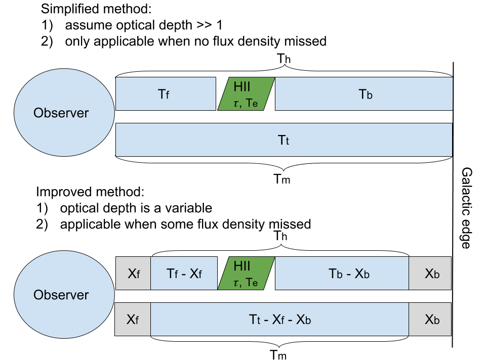
Secondly, the method underestimates the emissivity behind Hii regions when some flux density is resolved out by an interferometric observation, especially when the all-sky “zero-spacing" component is omitted (see Fig. 1). The shortest spacing of the MWA tiles is about 7 metres, corresponding to an angular scale of about 30 degrees, indicating that the MWA is sensitive to the whole sky emission with fluctuations on scales smaller than 30 degrees. Structures on larger angular scales are resolved out by the MWA. This undetected emission has the effect that the derived emissivities are under-estimated. The surface brightness of the Galactic synchrotron emission increases towards lower frequencies, making its contribution large at the 100 MHz frequencies relevant to the detection of Hii regions compared to 408 MHz at which the Haslam map was obtained.
To improve this method, we have developed a procedure that attempts to solve for both the optical depth of the Hii regions and the brightness temperature of the emission associated with the missing interferometric spacings. We scale the 408 MHz all-sky image to the frequency of interest by a global brightness temperature spectral index (: ) to estimate the total power along the line of sight and then use it to deduce the brightness temperature on scales resolved out by our interferometer. We use two data sets from the GLEAM survey with each one containing three frequencies (76.2, 83.8, 91.5 MHz; and 99.2, 106.9, 114.6 MHz ) to perform calculations and assume that synchrotron and optical depths have a power law scaling with the frequency. More details of this new method are described in what follows.
3.1 Definition of parameters
Fig. 1 shows a schematic of the absorption process, indicating the variables needed to solve for the emissivity. As usual, we assume the Galactic synchrotron emission is confined to an axisymmetric cylinder with a radius of 20 kpc and a height of several kpc. Note that this assumption is only for the definition of the emissivity in Section 3.2.1. We can avoid making this assumption if we are only interested in the brightness temperature instead of the emissivity.
The measured or known parameters are the measured brightness temperature in the direction of the absorbed region , the measured brightness temperature from the Sun to the Galactic edge in the absence of Hii region emission (i.e. as derived from a region near the line of sight to the Hii region), the observation frequency , the spectral index of the synchrotron brightness temperature , the spectral index of the Hii region optical depth , the total brightness temperature (without missing flux density) from the Sun to the Galactic edge in the absence of Hii region absorption , and the electron temperature of the Hii region . is taken to be for the Milky Way (Guzmán et al., 2011; Zheng et al., 2017). Note that this spectral index varies between -2.1 and -2.7 depending on the sky regions (Guzmán et al., 2011). We use a low spectral index of -2.7 for the synchrotron emission in this work because the high spectral index is due to the thermal free-free absorption of both the Hii regions and warm interstellar medium. is taken to be -2.1 for frequencies ( is in GHz and is in K) and K derived on page 47 of Lang (1980), which is always true for Hii regions at the GLEAM frequencies. Note that is a constant does not mean the Hii region must be optically thick; it can be optically thin. The errors caused by these two spectral indices are discussed in Section 4.3. is derived from the improved Haslam map (Remazeilles et al., 2015), scaled from 408 MHz to the GLEAM frequencies using the spectral index of . is from Balser et al. (2015); Hou & Han (2014) and references therein.
The unknown variables are the optical depth of the Hii region , the total (the sum of the measured and missed) brightness temperature of the synchrotron emission from the Hii region to the Galactic edge along the line of sight , and the corresponding brightness temperature of the synchrotron emission from the Hii region to the Sun , the brightness temperature of the emission on the missing short interferometric spacings respectively between an Hii region and the Sun , and between the Galactic edge and the Sun .
The selection criteria of the absorbed region and its nearby background region are the same as those in Su et al. (2017a). We define these regions at the lowest frequency of 76.2 MHz and then apply them to all other five frequencies to get the brightness temperatures within these regions. Hii regions overlapped with supernova remnants are not selected (e.g. Hii region G35.60.5 with distance measured by Zhu et al. 2013). Note that our selected background regions are about one degree away from the absorbed regions, the supernova remnants in Green (2014) catalogue, and obvious point-like sources in the GLEAM survey. Therefore, the contamination of these sources is negligible, although the Haslam map has a low angular resolution of 51′.
3.2 Equations to solve for the optical depth and brightness temperature
A single-dish observation can recover the total power along the line of sight in the case that the Hii region fills the beam. The brightness temperature is a result of the contributions from three components: the electron temperature of the Hii region, and the brightness temperature of the synchrotron emission behind and in front of the Hii region (Kassim, 1987),
| (1) |
An interferometer observation does not sample the large angular scale structures corresponding to visibility measurements at small - distances. Thus Equation 1 should be revised by subtracting the missing term from the brightness temperature both behind and in front of the Hii region,
| (2) |
Note that this equation does not require the - coverage to be identical at different frequencies because we do not assume the brightness temperature of the missing term follows the same spectral index. We allow the value of the X terms to float with frequency, as X depends on the angular scale at which emission is being missed, which varies with frequency.
The total brightness temperature from the Sun to the Galactic edge in the absence of Hii region absorption is simply the sum of the brightness temperatures behind and in front of the Hii region,
| (3) |
The measured brightness temperature on the source-free region (i.e. immediately adjacent to the Hii region) becomes the difference between the total brightness temperature and that of the brightness temperatures of the emission associated with the missing interferometric - spacings,
| (4) |
As well as the above three relations, we have supplementary information that encodes the scaling of the brightness temperature and the optical depth with frequency. The total brightness temperature both behind and in front of the Hii region should follow a power law distribution,
| (5) | ||||
We apply Equations (2)-(5) to our measurements at different frequencies to solve for the optical depth of Hii regions and the brightness temperatures behind and in front of each Hii region. In summary, we have:
| (6) | ||||
where the subscript indexes the frequencies from low to high. A minimum of three frequencies is required to solve for the unknown variables.
We derive the value of , , , , using Equation 6. Using two sets of three frequencies data, we obtain emissivities at the six frequencies listed in Table 1. We use data at 76.2, 83.8, and 91.5 MHz to derive the emissivites at these three frequencies. And then use another three frequencies of 99.2, 106.9, and 114.6 MHz to perform the same analysis. So we derive the emissivities at six different frequencies. Table LABEL:tab:emi lists the emissivities at 76.2 MHz only. We did not use other combinations of data to derive emissivities. We can derive and using the Haslam map to estimate the total emission along the line of sight. We then compare this total emission with that measured. Therefore, our equations can find out how much emission is undetected in our observations.
3.2.1 Definition of emissivity
The emissivity is defined to be the brightness temperature divided by the corresponding distance, i.e.,
| (7) | ||||
where is the average emissivity between the Hii region and the Galactic edge, is the average emissivity between the Hii region and the Sun, is the distance from the Hii region to the Galactic edge, and is the distance from the Hii region to the Sun. The value of is derived from Anderson et al. (2014); Anderson et al. (2017); Balser et al. (2015); Hou & Han (2014). The value of is calculated from assuming a Galactocentric radius of 20 kpc.
4 Results
4.1 Emissivities from simplified equations
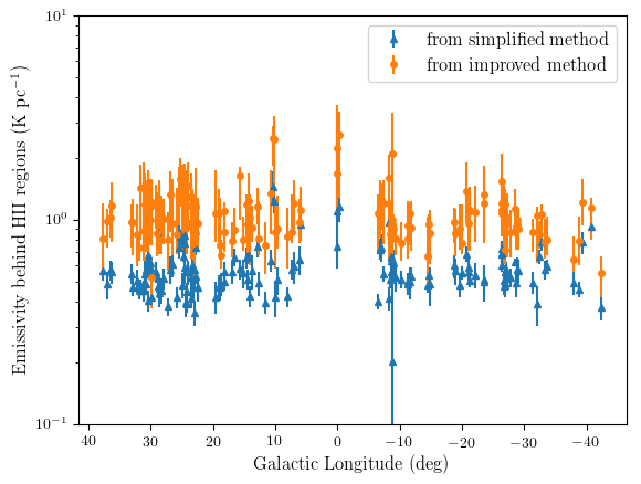
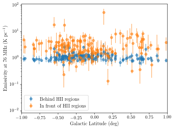
We calculate the synchrotron emissivities behind Hii regions using the 152 Hii region absorption features detected in the GLEAM survey using the previous simplified method (Col. 11 in Table LABEL:tab:emi). The last column in Table LABEL:tab:emi shows the emissivities derived from the simplified method described in Su et al. (2017a). The measurements are made at six frequencies from 76.2 to 114.6 MHz. The emissivities behind Hii regions at 76.2 MHz are plotted in Fig. 2. The derived emissivities in the fourth Galactic quadrant are consistent with our previous results in Su et al. (2017a, b). The emissivities in the first quadrant are consistent with those in Nord et al. (2006) within three standard deviations.
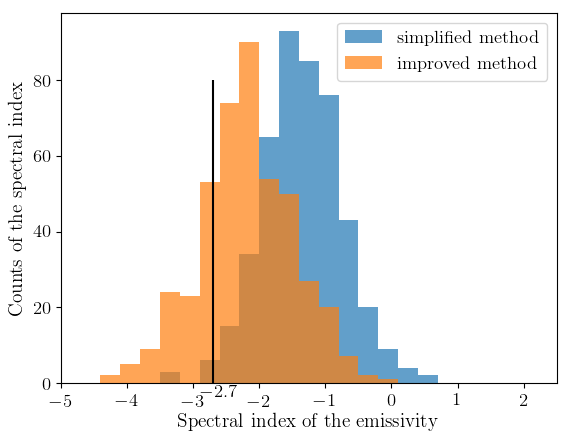
We check the spectral index of the emissivities at six frequencies derived from each Hii region. The average index is about -1.5, which is higher than the expected synchrotron emission spectral index of -2.7 (see Fig. 3). The difference between these observed two spectral indexes is most likely caused by the missing flux density mentioned in Section 3. To produce a flat spectrum with a spectral index of -1.5, the brightness temperature of the emission on scales that are resolved out should be frequency-dependent, with brightness temperatures under-estimated at lower frequencies in our observations, even though our lower frequencies recover more of the extended emission than the high frequencies: this demonstrates that we need to improve this simplified method to derive more accurate emissivities.
4.2 Emissivities derived from our new method
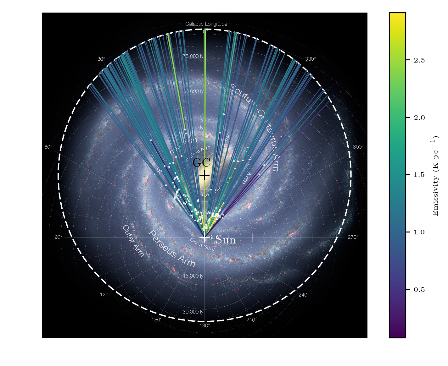
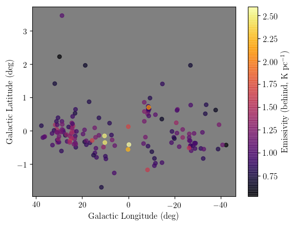
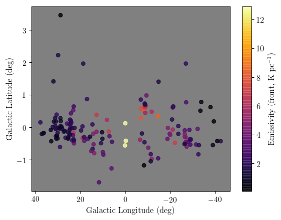
Using the improved method described in Section 3, we obtained the synchrotron emissivities and Hii region optical depths at six frequencies simultaneously (see Table LABEL:tab:emi). Fig. 4 shows the emissivities at 76.2 MHz and the paths over which these emissivities are averaged. The electronic version of the full tables with our derived emissivities at all six frequencies is available from VizieR. Figs. 5 and 6 show our derived emissivities at 76.2 MHz both behind and in front of Hii regions using the improved method.
4.3 Error estimation
For the emissivities derived from simplified equations, we propagate the error throughout the simple equations to estimate their errors. For our improved method, the equations are too complex to permit directly calculating the uncertainty of each solution caused by the variance of the known parameters from the measurements. The sources of the error include
-
•
the error of the Hii region electron temperature,
-
•
the error of the distance from Hii region to us,
-
•
the rms of the brightness temperature for the absorbed region in the GLEAM map,
-
•
the rms of the brightness temperature for the background region in the GLEAM map,
-
•
the rms of the brightness temperature for the background region in the Haslam map,
-
•
the variation of the spectral indices of the synchrotron brightness temperature and the Hii region optical depth.
We use a Monte Carlo method to statistically estimate the error of these solutions caused by the first five error sources. Specifically, we use the values of known parameters to calculate the solutions and then sample around these parameters. We set each input parameter to be a random number following a Gaussian distribution with a mean from the best input value and a standard derivation from our one-sigma measurement error. Using these new input parameters, we can find new solutions. By repeating the calculation, we get a distribution of each solution and then calculate the one-sigma upper and lower limits. The estimated errors are about 10-90% of the emissivity values (see Table LABEL:tab:emi). Note that we do not include the contribution of the spectral indices of the synchrotron brightness temperature and the Hii region optical depth because finding the solutions becomes computationally expensive with these two spectral indices included. The spectral index of the brightness temperature cause a difference of about 15% of the emissivity values, estimated from the variance of the Haslam map scaling, when this spectral index changes from -2.7 to -2.6. Although this causes extra error to the derived emissivities, it is still necessary to use the Haslam map; otherwise, the derived emissivities behind the Hii regions will be under-estimated due to the missing flux density, and the emissivities in front of Hii regions cannot be calculated. The error contributed by the spectral index of the Hii region optical depth is small ( 1% of the emissivity) because the term in Equation 6 is small when the optical depth is much larger than one.
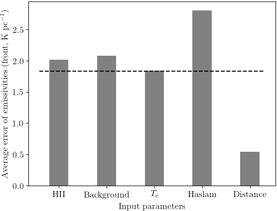
We check which input parameter dominates the errors of the final emissivities. We set only one input parameter to be a random number while setting all other parameters to be constants. Then, similarly to the above error estimation, we calculate the one-sigma upper and lower limits of the emissivities. The error contribution of each input parameter is shown in Fig. 7. We find the rms of the brightness temperature of the Haslam map contributes the most to the final errors of the derived emissivities.
In the future, new maps using new data processing techniques may be able to recover the total power along the line of sight, which will avoid extrapolating the Halam map from 408 MHz to the GLEAM frequencies. For example, Eastwood et al. (2017) use a new widefield imaging technique, named the Tikhonov-regularized m-mode analysis imaging to map the northern sky with most of the large-scale structures recovered. The lunar occultation technique enables measuring the Galactic synchrotron emission integrated along the line of sight where the Moon occults the sky (e.g. Shaver et al. 1999; McKinley et al. 2013 and McKinley et al. submitted). Future large single-dishes observing at around 150 MHz will assist further.
5 Discussion of the derived emissivities
We compare the emissivities from the simplified method and our improved method in Fig. 2 (left). The emissivities from the old method are systematically lower than those from the new method, which indicates the old method underestimates the emissivities due to the missing flux density.
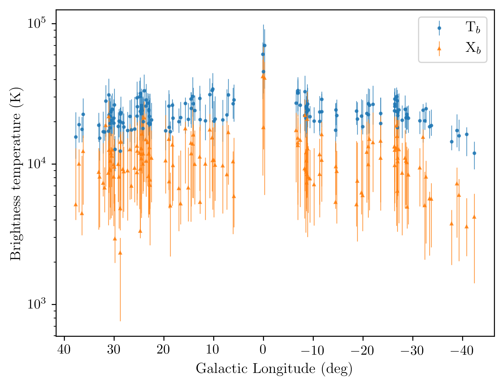
We compare the total and missing brightness temperatures behind the Hii region in Fig. 2 (right). The unrecovered brightness temperature behind Hii regions () is about 50% of the total brightness temperature behind Hii regions (), indicating that about 50% of the large-scale structure behind Hii regions has not been recovered in our observations. The brightness temperature in front of Hii regions that was not recovered () is comparable with the total brightness temperature in front of Hii regions () indicating that nearly all the large-scale structures in front of Hii regions have not been recovered. Thus, the missing structures must be considered in the emissivity calculation. Note that the and are comparable, while is about 50% of . It is reasonable that most of are not detected because an interferometer measures the difference along the Hii region direction and its nearby direction, and also because most Hii regions are nearby so that accumulated is small compared to . The emission from the Hii region to us is nearly the same for both directions, therefore, is not easily detected. However, is ‘different’ on the Hii region direction and its nearby direction because most of the is absorbed by the Hii region on its direction, so the MWA detects a portion of .
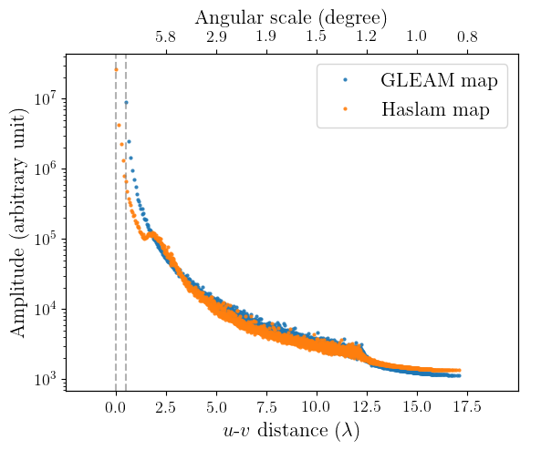
To confirm that the portion of missing detection is reasonable, we compare the GLEAM map and the Haslam map at the visibility plane. We use nine square regions with size of 10∘, 30∘, and 60∘ centred at , , and , . We use the GLEAM map at the frequency of 76.2 MHz. The Haslam map is scaled from 408 MHz to the same frequency of 76.2 MHz using a spectral index of -2.7. The GLEAM map is smoothed to the same angular resolution of the Haslam map (51 arcmin), and the two maps are made with the same pixel size. For each region, we convert the two images to the visibility plane using Fast Fourier Transform (FFT) and then plot the amplitude against - distance to compare the difference between the two visibilities (see Fig. 8). The difference varies with the region size and location. On average, about 60% of the amplitude in the visibility of the Haslam map is not detected in the GLEAM survey. Our absorption analysis shows that 50% of the large-scale structures are not recovered for the emission behind Hii regions, and nearly all emission from the column between the Hii region and the Sun is not detected. These two results are generally consistent.
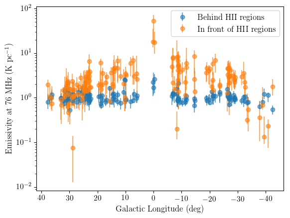
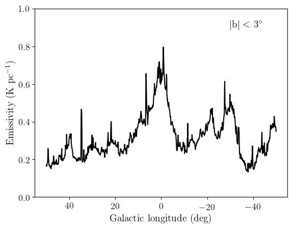
The most apparent feature in the derived emissivities is that they increase towards the Galactic centre. Both the emissivity and the brightness temperature peak near the Galactic centre and decrease as the line-of-sight goes far away from the Galactic centre (Fig. 2). To further confirm this trend, we check the average emissivity measured in the GLEAM map from the Sun to the Galactic edge (Fig. 9). It is evident that the emissivity along the path from the Sun to the Galactic edge peaks at the Galactic centre direction. This trend indicates the emissivity decreases with Galactocentric radius, which is modelled in Su et al. (2017a, b). This is consistent with the lowest order of disk component of the Galactic magnetic field, which is usually assumed to be exponentially distributed in the previous models (e.g. Beuermann et al. 1985; Sun et al. 2008). Face-on galaxies with spiral arms directly observed also show a similar profile as the one in Fig. 9, e.g. the LOw Frequency ARray (LOFAR; van Haarlem et al. 2013) observation of the Whirlpool Galaxy (also known as M51) at the frequency of 150 MHz (see Fig. 13 in Mulcahy et al. 2014).
The average emissivities along the paths near the line of sight to the Sun are much higher than those far away from the Sun, though they have large errors. Several reasons can explain this effect. Firstly, the emissivity near the Galactic edge is much lower than that near the Galactic centre, which makes our average emissivities along the path high near the Galactic centre and low near the Galactic edge. Secondly, it may simply indicate that all distances from the Hii region to the Galactic edge along the line of sight are over-estimated, which makes the emissivities behind Hii regions decrease fractionally with distance. Thirdly, it may indicate the region near the Sun is not a representative region of the whole Milky Way because previous studies show that we are in a local bubble created by two or three supernovae (Maíz-Apellániz, 2001), which may increase the density of cosmic-ray electrons within several kpc of the Sun.
No obvious spiral arm structures can be visually seen from our observed emissivities because the emissivity is averaged along different path lengths. Further modelling work in the future will help to reveal that whether the emissivity distribution is correlated with the spiral arms or not, because this information is embedded in our derived emissivities. From an observational aspect, we can see the spiral arms as peaks in emissivity and brightness temperature along the total paths from the Sun to the Galactic edge as a function of Galactic longitude (see Fig. 6 in Su et al. 2017a and Fig. 1 in Beuermann et al. 1985).
We estimate the number density of relativistic electrons in the Galactic disk to confirm that our derived emissivities are consistent with existing electron models. Specifically, we get the relativistic electron density by using the total power of the synchrotron emission in the Galactic disk divided by the total power of one relativistic electron and then divided by the volume of the Galactic disk. In the above calculations, we use an average Galactic magnetic field strength of G (Sun et al., 2008) and an average emissivity of 1 0.5 K pc-1 at 76.2 MHz where 1 K pc-1 is equal to 5.7510-41 W m-3 Hz-1 sr-1. We use a typical energy of relativistic electrons of 10 1 GeV (Stephens, 2001), a radius of the Galactic disk of 20 kpc (Nord et al., 2006), and scale height of the Galactic disk of 1 kpc. We integrate the power of synchrotron emission in the frequency range 10 MHz to 1000 GHz. We derive a number density of relativistic electrons of 168 108 cm-3. The relativistic electrons follow a power law distribution with energy, ne(E) = k E-3.152 (Adriani et al., 2017). Using this distribution, we derive the average density of 10 GeV electrons to be (5.6 3.6) 10-5 cm-3, which is similar to the value of () cm-3 from the literature (see Fig. 4 in Jansson & Farrar 2012, cited from GALPROP in Strong et al. 2010). Note that the estimated electron density has large errors due to the above typical values adopted. To further investigate the electron distribution, future work should use comprehensive Galactic magnetic field models (Han et al., 2006; Brown et al., 2007; Sun et al., 2008; Sun & Reich, 2010; Van Eck et al., 2011).
6 Summary
We develop a new method of emissivity calculation by improving upon the previous simplified method. Using this new method, we calculate the synchrotron emissivities both behind and in front of 152 Hii regions at six frequencies of 76.2, 83.8, 91.5, 99.2, 106.9, and 114.6 MHz. This new method enables us to derive the Hii region optical depth and estimate the amount of flux density missing from our observations at each frequency. We find that the emissivities increase towards the Galactic centre. This lowest order of emissivity variation is consistent with the current Galactic magnetic field and relativistic electron distributions because both the magnetic field strength and the relativistic electron density increase towards the Galactic centre. The high emissivities nearby the Sun (if actually real) might be caused by the local bubble.
The number of line-of-sight measurements will increase in the MWA phase II stage (Wayth et al., in prep.) because both the number of antenna and the maximum baselines are increased, and in the future, we will have better knowledge of the distance and electron temperature of Hii regions. The lack of Hii regions with larger distances is a key factor holding back the modelling at present because most Hii regions are located near the Sun with distances less than several kpc. Future total power surveys at similar frequencies can improve the accuracy of the emissivity measurements. The derived emissivities may help to recover the 3-D distribution of synchrotron emission in the Milky Way. Furthermore, they provide direct information on the spatial distribution of the Galactic magnetic field and the relativistic electrons for the future modelling.
Acknowledgements
This scientific work makes use of the Murchison Radio-astronomy Observatory, operated by CSIRO. We acknowledge the Wajarri Yamatji people as the traditional owners of the Observatory site. Support for the operation of the MWA is provided by the Australian Government (NCRIS), under a contract to Curtin University administered by Astronomy Australia Limited. We acknowledge the Pawsey Supercomputing Centre which is supported by the Western Australian and Australian Governments. HS & WWT thanks the support from the NSFC (11473038, 11273025). This research utilized Astropy (Astropy Collaboration et al., 2013), Scipy (Jones et al., 2001), Numpy (Van Der Walt et al., 2011), and Matplotlib (Hunter, 2007). We thank the anonymous referee and Denis Leahy for helpful comments.
References
- Adriani et al. (2017) Adriani O., et al., 2017, Physical Review Letters, 119, 181101
- Anderson et al. (2014) Anderson L. D., Bania T. M., Balser D. S., Cunningham V., Wenger T. V., Johnstone B. M., Armentrout W. P., 2014, ApJS, 212, 1
- Anderson et al. (2015) Anderson L. D., Armentrout W. P., Johnstone B. M., Bania T. M., Balser D. S., Wenger T. V., Cunningham V., 2015, ApJS, 221, 26
- Anderson et al. (2017) Anderson L. D., Armentrout W. P., Luisi M., Bania T. M., Balser D. S., Wenger T. V., 2017, preprint, (arXiv:1710.07397)
- Armentrout et al. (2017) Armentrout W. P., Anderson L. D., Balser D. S., Bania T. M., Dame T. M., Wenger T. V., 2017, ApJ, 841, 121
- Astropy Collaboration et al. (2013) Astropy Collaboration et al., 2013, A&A, 558, A33
- Balser et al. (2015) Balser D. S., Wenger T. V., Anderson L. D., Bania T. M., 2015, ApJ, 806, 199
- Beuermann et al. (1985) Beuermann K., Kanbach G., Berkhuijsen E. M., 1985, A&A, 153, 17
- Bowman et al. (2013) Bowman J. D., et al., 2013, Publ. Astron. Soc. Australia, 30, 31
- Brown et al. (2007) Brown J. C., Haverkorn M., Gaensler B. M., Taylor A. R., Bizunok N. S., McClure-Griffiths N. M., Dickey J. M., Green A. J., 2007, ApJ, 663, 258
- Burke (1957) Burke B. F., 1957, AJ, 62, 90
- Dickinson et al. (2003) Dickinson C., Davies R. D., Davis R. J., 2003, MNRAS, 341, 369
- Eastwood et al. (2017) Eastwood M. W., et al., 2017, preprint, (arXiv:1711.00466)
- Green (2014) Green D. A., 2014, Bulletin of the Astronomical Society of India, 42, 47
- Guzmán et al. (2011) Guzmán A. E., May J., Alvarez H., Maeda K., 2011, A&A, 525, A138
- Han et al. (2006) Han J. L., Manchester R. N., Lyne A. G., Qiao G. J., van Straten W., 2006, ApJ, 642, 868
- Hancock et al. (2012) Hancock P. J., Murphy T., Gaensler B. M., Hopkins A., Curran J. R., 2012, MNRAS, 422, 1812
- Hancock et al. (2018) Hancock P. J., Trott C. M., Hurley-Walker N., 2018, Publ. Astron. Soc. Australia, 35, e011
- Haslam et al. (1981) Haslam C. G. T., Klein U., Salter C. J., Stoffel H., Wilson W. E., Cleary M. N., Cooke D. J., Thomasson P., 1981, A&A, 100, 209
- Haslam et al. (1982) Haslam C. G. T., Salter C. J., Stoffel H., Wilson W. E., 1982, A&AS, 47, 1
- Hindson et al. (2016) Hindson L., et al., 2016, Publ. Astron. Soc. Australia, 33, e020
- Hou & Han (2014) Hou L. G., Han J. L., 2014, A&A, 569, A125
- Hunter (2007) Hunter J. D., 2007, Computing in Science and Engineering, 9, 90
- Hurley-Walker et al. (2017) Hurley-Walker N., et al., 2017, MNRAS, 464, 1146
- Jansson & Farrar (2012) Jansson R., Farrar G. R., 2012, ApJ, 757, 14
- Jones et al. (2001) Jones E., Oliphant T., Peterson P., others 2001, SciPy: Open source scientific tools for Python
- Kassim (1987) Kassim N. E. S., 1987, PhD thesis, Maryland Univ., College Park.
- Kerr (1957) Kerr F. J., 1957, AJ, 62, 93
- Lang (1980) Lang K. R., 1980, Astrophysical Formulae. A Compendium for the Physicist and Astrophysicist.
- Maíz-Apellániz (2001) Maíz-Apellániz J., 2001, ApJ, 560, L83
- McKinley et al. (2013) McKinley B., et al., 2013, AJ, 145, 23
- Mulcahy et al. (2014) Mulcahy D. D., et al., 2014, A&A, 568, A74
- Nord et al. (2006) Nord M. E., Henning P. A., Rand R. J., Lazio T. J. W., Kassim N. E., 2006, AJ, 132, 242
- Offringa et al. (2014) Offringa A. R., et al., 2014, MNRAS, 444, 606
- Remazeilles et al. (2015) Remazeilles M., Dickinson C., Banday A. J., Bigot-Sazy M.-A., Ghosh T., 2015, MNRAS, 451, 4311
- Shaver et al. (1999) Shaver P. A., Windhorst R. A., Madau P., de Bruyn A. G., 1999, A&A, 345, 380
- Stephens (2001) Stephens S. A., 2001, Advances in Space Research, 27, 687
- Strong et al. (2010) Strong A. W., Porter T. A., Digel S. W., Jóhannesson G., Martin P., Moskalenko I. V., Murphy E. J., Orlando E., 2010, ApJ, 722, L58
- Su et al. (2017a) Su H., et al., 2017a, MNRAS, 465, 3163
- Su et al. (2017b) Su H., et al., 2017b, MNRAS, 472, 828
- Sun & Reich (2010) Sun X.-H., Reich W., 2010, Research in Astronomy and Astrophysics, 10, 1287
- Sun et al. (2008) Sun X. H., Reich W., Waelkens A., Enßlin T. A., 2008, A&A, 477, 573
- Tingay et al. (2013) Tingay S. J., et al., 2013, Publ. Astron. Soc. Australia, 30, 7
- Van Der Walt et al. (2011) Van Der Walt S., Colbert S. C., Varoquaux G., 2011, preprint, (arXiv:1102.1523)
- Van Eck et al. (2011) Van Eck C. L., et al., 2011, ApJ, 728, 97
- Wayth et al. (2015) Wayth R. B., et al., 2015, Publ. Astron. Soc. Australia, 32, e025
- Zheng et al. (2017) Zheng H., et al., 2017, MNRAS, 464, 3486
- Zhu et al. (2013) Zhu H., Tian W. W., Torres D. F., Pedaletti G., Su H. Q., 2013, ApJ, 775, 95
- de Oliveira-Costa et al. (2008) de Oliveira-Costa A., Tegmark M., Gaensler B. M., Jonas J., Landecker T. L., Reich P., 2008, MNRAS, 388, 247
- van Haarlem et al. (2013) van Haarlem M. P., et al., 2013, A&A, 556, A2
| Hii region | Dis | |||||||||||||
|---|---|---|---|---|---|---|---|---|---|---|---|---|---|---|
| kpc | 103 K | 103 K | 103 K | 103 K | 103 K | 103 K | 103 K | 103 K | K pc-1 | K pc-1 | K pc-1 | |||
| (1) | (2) | (3) | (4) | (5) | (6) | (7) | (8) | (9) | (10) | (11) | (12) | (13) | (14) | |
| G000.00300.127 | 1.5 0.3 | 7.62 0.30 | 17.0 1.0 | 36.7 4.7 | 124.9 10.6 | 45.6 | 79.4 | 18.2 | 70.0 | 36.3 | 1.7 | 52.9 | 1.10 0.20 | |
| G000.12000.556 | 1.5 0.3 | 7.62 0.30 | 23.5 2.3 | 34.5 3.3 | 87.4 20.0 | 60.5 | 26.9 | 41.8 | 11.0 | 30.0 | 2.2 | 17.9 | 0.74 0.17 | |
| G005.88700.443 | 3.0 0.2 | 11.13 0.20 | 7.5 3.1 | 19.1 0.8 | 40.3 2.2 | 28.6 | 7.9 | 5.9 | 15.4 | 39.2 | 1.1 | 2.6 | 0.95 0.14 | |
| G006.10001.263 | 1.0 0.2 | 7.70 0.80 | 1.6 0.7 | 10.4 2.2 | 30.3 2.6 | 26.9 | 3.4 | 10.4 | 9.5 | 45.6 | 1.0 | 3.4 | 0.64 0.10 | |
| G007.01500.271 | 2.7 0.5 | 7.50 0.80 | 7.9 1.9 | 14.8 1.2 | 39.2 3.8 | 31.0 | 8.2 | 16.7 | 7.8 | 23.2 | 1.2 | 3.0 | 0.59 0.10 | |
| G007.30300.125 | 2.7 0.5 | 7.17 0.30 | 8.2 0.7 | 14.9 1.2 | 40.8 4.7 | 22.3 | 18.5 | 8.4 | 17.5 | 6.3 | 0.9 | 6.8 | 0.57 0.06 | |
| G008.13700.232 | 3.4 0.8 | 7.09 0.10 | 11.6 0.5 | 14.7 0.9 | 40.5 2.5 | 20.6 | 19.9 | 9.7 | 15.9 | 99 | 0.8 | 5.9 | 0.42 0.05 | |
| G009.72500.840 | 5.2 1.0 | 6.27 0.30 | 10.2 0.5 | 15.1 1.5 | 37.5 3.6 | 21.0 | 16.5 | 9.8 | 12.6 | 99 | 0.9 | 3.2 | 0.51 0.08 | |
| G009.94200.761 | 5.2 1.0 | 3.70 0.40 | 10.4 0.5 | 15.8 1.6 | 38.7 3.3 | 20.2 | 17.9 | 10.7 | 11.6 | 7.4 | 0.9 | 3.5 | 0.42 0.08 | |
| G010.16000.350 | 14.5 0.9 | 6.83 0.00 | 7.8 0.9 | 16.9 1.4 | 41.2 1.3 | 34.2 | 14.7 | 10.6 | 13.7 | 6.3 | 2.5 | 1.0 | 1.23 0.16 | |
| G010.30800.150 | 15.0 1.1 | 6.80 0.00 | 10.0 0.4 | 21.3 2.9 | 45.4 0.6 | 33.4 | 12.0 | 15.4 | 8.7 | 58.7 | 2.5 | 0.8 | 1.46 0.27 | |
| G010.76900.487 | 5.0 1.0 | 5.30 0.50 | 8.6 0.7 | 17.1 1.3 | 41.6 2.5 | 31.3 | 10.3 | 17.5 | 7.0 | 15.8 | 1.3 | 2.1 | 0.63 0.08 | |
| G011.66201.692 | 1.2 0.1 | 7.75 0.30 | 4.7 0.2 | 7.3 1.1 | 24.0 1.5 | 20.4 | 3.6 | 10.0 | 6.7 | 12.4 | 0.8 | 3.0 | 0.39 0.05 | |
| G012.74200.390 | 2.6 0.7 | 7.23 0.30 | 11.0 0.8 | 15.8 1.2 | 38.3 2.8 | 20.7 | 17.6 | 5.3 | 17.2 | 99 | 0.8 | 6.8 | 0.49 0.07 | |
| G012.76100.133 | 2.9 0.3 | 7.62 0.10 | 2.6 1.0 | 12.5 1.6 | 42.5 1.1 | 29.3 | 13.2 | 11.2 | 18.3 | 9.8 | 1.2 | 4.6 | 0.74 0.08 | |
| G013.77600.795 | 2.0 0.4 | 8.60 0.90 | 6.0 0.6 | 11.4 2.2 | 33.4 3.5 | 24.0 | 9.4 | 9.9 | 12.0 | 99 | 0.9 | 4.7 | 0.56 0.11 | |
| G014.06000.521 | 2.0 0.4 | 7.46 0.30 | 7.2 0.4 | 10.4 1.0 | 34.6 3.9 | 26.8 | 7.8 | 16.1 | 8.0 | 99 | 1.0 | 3.9 | 0.42 0.05 | |
| G014.20700.193 | 3.6 0.5 | 6.89 0.30 | 4.3 0.9 | 13.0 1.1 | 46.9 2.5 | 30.3 | 16.2 | 13.9 | 19.8 | 15.6 | 1.2 | 4.5 | 0.67 0.07 | |
| G014.48100.662 | 2.0 0.4 | 10.40 1.00 | 6.9 0.5 | 9.6 0.9 | 28.5 2.2 | 24.9 | 3.6 | 11.8 | 7.1 | 79.6 | 1.0 | 1.8 | 0.51 0.06 | |
| G014.57600.091 | 3.6 0.5 | 5.51 0.10 | 3.1 1.5 | 12.6 0.7 | 36.4 2.4 | 29.1 | 7.3 | 14.1 | 9.7 | 66.2 | 1.2 | 2.0 | 0.66 0.08 | |
| G015.09700.729 | 2.0 0.1 | 9.77 0.10 | 4.6 1.6 | 8.7 1.3 | 28.1 4.8 | 20.8 | 7.3 | 6.8 | 12.6 | 99 | 0.8 | 3.7 | 0.55 0.09 | |
| G015.67600.288 | 11.6 0.4 | 6.51 0.30 | 8.4 0.2 | 11.1 0.9 | 36.8 0.3 | 27.0 | 9.8 | 17.8 | 7.9 | 15.0 | 1.6 | 0.8 | 0.58 0.06 | |
| G016.64800.357 | 3.9 0.4 | 6.81 0.30 | 4.6 1.0 | 12.7 0.9 | 33.1 0.8 | 21.4 | 11.7 | 5.2 | 15.2 | 99 | 0.9 | 3.0 | 0.66 0.06 | |
| G016.99300.873 | 2.6 0.5 | 6.97 0.10 | 1.5 0.5 | 7.8 1.5 | 25.7 3.1 | 20.0 | 5.7 | 6.7 | 11.2 | 19.4 | 0.8 | 2.2 | 0.55 0.07 | |
| G018.18700.415 | 3.6 0.4 | 6.93 0.30 | 8.0 0.4 | 12.5 0.8 | 33.9 0.9 | 21.3 | 12.6 | 9.7 | 11.6 | 10.8 | 0.9 | 3.5 | 0.50 0.04 | |
| G018.25300.298 | 4.1 0.4 | 7.18 0.10 | 6.9 1.2 | 12.3 0.9 | 34.3 0.4 | 26.2 | 8.1 | 13.7 | 8.3 | 24.0 | 1.1 | 2.0 | 0.56 0.07 | |
| G018.66901.965 | 2.6 0.5 | 7.21 0.10 | 1.2 0.8 | 5.8 1.2 | 21.0 2.8 | 17.0 | 4.0 | 5.0 | 10.3 | 32.6 | 0.7 | 1.5 | 0.49 0.06 | |
| G018.91400.329 | 3.4 0.7 | 5.44 0.10 | 5.7 0.8 | 11.0 1.1 | 38.9 1.2 | 18.3 | 20.6 | 7.5 | 20.4 | 39.8 | 0.7 | 6.1 | 0.47 0.06 | |
| G018.97800.030 | 4.0 0.4 | 6.81 0.30 | 7.8 1.1 | 11.8 0.7 | 33.9 0.4 | 25.8 | 8.1 | 15.0 | 7.1 | 18.0 | 1.1 | 2.0 | 0.47 0.06 | |
| G019.62900.095 | 11.7 0.4 | 6.48 0.10 | 10.9 0.1 | 11.1 1.0 | 39.5 1.0 | 17.3 | 22.3 | 10.5 | 17.9 | 78.6 | 1.1 | 1.9 | 0.42 0.07 | |
| G022.47800.015 | 6.2 1.2 | 6.33 0.30 | 8.6 0.7 | 11.9 0.9 | 31.9 1.8 | 20.7 | 10.8 | 11.0 | 9.4 | 75.5 | 1.0 | 1.7 | 0.47 0.07 | |
| G022.76100.492 | 4.8 0.4 | 6.65 0.30 | 6.8 0.3 | 11.6 0.7 | 37.9 1.7 | 19.5 | 18.4 | 7.1 | 19.2 | 62.6 | 0.9 | 3.8 | 0.53 0.04 | |
| G022.78000.401 | 11.1 0.4 | 6.71 0.30 | 6.8 0.3 | 11.6 0.7 | 37.9 1.7 | 19.2 | 18.7 | 7.7 | 18.6 | 7.0 | 1.2 | 1.7 | 0.73 0.06 | |
| G022.87900.645 | 2.5 0.5 | 7.34 0.30 | 9.8 0.3 | 11.1 0.9 | 28.0 2.0 | 21.9 | 6.1 | 13.1 | 3.8 | 99 | 0.9 | 2.4 | 0.35 0.05 | |
| G022.98700.155 | 2.5 0.5 | 5.10 0.50 | 9.9 0.3 | 17.0 1.0 | 40.2 2.1 | 24.0 | 16.2 | 11.8 | 11.4 | 44.2 | 1.0 | 6.5 | 0.52 0.05 | |
| G022.98800.360 | 4.8 0.4 | 6.66 0.30 | 6.1 0.8 | 11.7 0.8 | 39.1 1.8 | 24.4 | 14.4 | 11.9 | 15.4 | 13.0 | 1.1 | 3.0 | 0.57 0.06 | |
| G023.09700.527 | 2.4 0.5 | 7.38 0.30 | 7.3 0.4 | 11.2 1.1 | 27.9 2.0 | 19.4 | 8.4 | 8.1 | 8.5 | 11.9 | 0.8 | 3.5 | 0.47 0.05 | |
| G023.24000.240 | 4.8 0.4 | 6.66 0.30 | 10.7 0.8 | 17.0 1.0 | 40.2 2.1 | 27.2 | 13.0 | 14.2 | 9.0 | 52.6 | 1.2 | 2.7 | 0.60 0.07 | |
| G023.57200.020 | 5.5 0.4 | 6.51 0.30 | 6.7 0.4 | 9.0 0.7 | 36.3 1.1 | 28.6 | 7.7 | 10.5 | 16.8 | 99 | 1.3 | 1.4 | 0.41 0.04 | |
| G023.58100.400 | 5.4 0.4 | 6.53 0.30 | 8.1 0.3 | 12.6 1.5 | 40.3 1.9 | 25.9 | 14.8 | 14.9 | 13.1 | 13.8 | 1.2 | 2.7 | 0.52 0.08 | |
| G023.95700.149 | 4.9 0.4 | 6.66 0.30 | 7.3 0.3 | 12.6 1.5 | 40.3 1.9 | 33.3 | 7.0 | 21.4 | 6.3 | 60.3 | 1.5 | 1.4 | 0.56 0.08 | |
| G024.13900.432 | 5.8 0.5 | 6.46 0.30 | 8.0 0.2 | 9.8 0.6 | 37.3 1.0 | 20.0 | 17.3 | 11.8 | 15.7 | 11.0 | 0.9 | 3.0 | 0.39 0.04 | |
| G024.18500.211 | 9.1 0.7 | 6.37 0.30 | 8.2 0.1 | 9.8 0.6 | 37.3 1.0 | 18.0 | 19.3 | 10.0 | 17.6 | 11.7 | 1.0 | 2.1 | 0.45 0.05 | |
| G024.34700.088 | 8.5 0.9 | 6.31 0.30 | 6.4 0.2 | 7.4 0.9 | 42.3 0.2 | 24.0 | 18.3 | 16.4 | 18.5 | 99 | 1.3 | 2.2 | 0.39 0.06 | |
| G024.49300.219 | 9.7 0.5 | 6.48 0.30 | 2.9 0.4 | 10.3 0.8 | 39.2 1.0 | 25.0 | 13.8 | 10.9 | 17.9 | 64.8 | 1.4 | 1.4 | 0.84 0.06 | |
| G024.49800.039 | 9.2 0.6 | 6.40 0.30 | 5.8 0.2 | 12.6 1.4 | 40.2 1.9 | 26.1 | 13.7 | 12.9 | 14.7 | 34.2 | 1.4 | 1.5 | 0.77 0.09 | |
| G024.50700.239 | 8.8 2.8 | 6.36 0.10 | 5.3 0.1 | 9.4 0.8 | 37.4 1.3 | 22.8 | 14.5 | 11.7 | 15.7 | 20.5 | 1.2 | 1.6 | 0.59 0.10 | |
| G024.72400.084 | 9.1 0.7 | 6.40 0.30 | 2.8 0.5 | 9.9 1.1 | 39.4 1.3 | 23.7 | 16.1 | 3.3 | 26.1 | 6.0 | 1.3 | 1.8 | 0.78 0.08 | |
| G024.74300.210 | 5.1 0.4 | 6.63 0.30 | 3.0 0.3 | 10.4 0.8 | 39.2 1.0 | 31.8 | 7.3 | 9.2 | 19.5 | 29.7 | 1.4 | 1.4 | 0.67 0.05 | |
| G024.84400.093 | 6.3 0.6 | 5.86 0.10 | 6.3 0.4 | 10.1 1.2 | 39.5 1.3 | 30.1 | 9.4 | 11.9 | 17.1 | 39.4 | 1.4 | 1.5 | 0.48 0.07 | |
| G025.29100.303 | 11.2 0.4 | 6.87 0.30 | 4.5 0.5 | 10.3 0.8 | 39.2 1.0 | 25.6 | 13.4 | 12.3 | 16.0 | 7.5 | 1.6 | 1.2 | 0.83 0.07 | |
| G025.38200.151 | 4.0 0.4 | 9.28 0.10 | 4.1 0.7 | 11.0 1.5 | 32.3 2.1 | 29.6 | 6.7 | 13.4 | 12.0 | 12.0 | 1.3 | 1.7 | 0.73 0.08 | |
| G025.38600.347 | 11.2 0.4 | 6.88 0.30 | 4.6 0.4 | 11.0 1.5 | 32.3 2.1 | 22.0 | 10.3 | 8.7 | 12.6 | 17.5 | 1.4 | 0.9 | 0.87 0.11 | |
| G025.86700.118 | 6.5 0.9 | 6.12 0.10 | 7.2 0.5 | 9.5 0.7 | 36.1 1.3 | 17.8 | 18.4 | 9.4 | 17.3 | 50.1 | 0.9 | 2.8 | 0.42 0.05 | |
| G026.52100.317 | 9.1 0.6 | 6.50 0.30 | 7.0 0.2 | 11.0 1.2 | 33.8 1.7 | 17.5 | 16.3 | 7.0 | 15.8 | 15.1 | 1.0 | 1.8 | 0.61 0.08 | |
| G026.79700.113 | 10.8 0.4 | 6.85 0.30 | 6.9 0.7 | 9.2 1.1 | 35.2 1.1 | 21.8 | 13.0 | 12.6 | 12.9 | 99 | 1.3 | 1.2 | 0.57 0.09 | |
| G027.28100.132 | 5.5 0.5 | 6.62 0.30 | 7.4 0.2 | 8.8 0.6 | 28.3 1.7 | 17.3 | 10.7 | 8.9 | 9.8 | 67.8 | 0.8 | 1.9 | 0.38 0.04 | |
| G028.02200.043 | 9.0 0.6 | 6.57 0.30 | 6.4 0.7 | 8.8 0.6 | 28.3 1.7 | 18.4 | 10.3 | 8.8 | 10.8 | 8.5 | 1.0 | 1.1 | 0.52 0.06 | |
| G028.24600.013 | 7.5 1.5 | 6.48 0.30 | 7.8 0.3 | 9.9 0.9 | 30.9 1.6 | 19.6 | 11.3 | 9.2 | 11.9 | 91.0 | 1.0 | 1.5 | 0.45 0.06 | |
| G028.63800.194 | 7.5 1.5 | 6.50 0.30 | 7.7 0.4 | 9.9 0.9 | 30.9 1.6 | 23.2 | 7.7 | 14.5 | 6.5 | 15.8 | 1.2 | 1.0 | 0.46 0.07 | |
| G028.67900.044 | 7.5 1.6 | 6.50 0.30 | 8.0 0.1 | 9.9 0.9 | 30.9 1.6 | 22.7 | 8.3 | 14.3 | 6.7 | 14.4 | 1.2 | 1.1 | 0.44 0.06 | |
| G028.74603.458 | 15.2 0.8 | 8.30 0.40 | 0.1 0.8 | 1.9 0.8 | 12.5 0.8 | 12.4 | 1.1 | 2.3 | 8.3 | 18.1 | 1.0 | 0.1 | 0.87 0.13 | |
| G028.77400.285 | 7.4 1.5 | 6.50 0.30 | 7.5 0.2 | 10.0 0.9 | 30.4 1.7 | 20.0 | 10.8 | 4.8 | 15.5 | 14.2 | 1.0 | 1.5 | 0.48 0.06 | |
| G028.98300.604 | 3.5 0.4 | 7.12 0.30 | 5.3 0.3 | 10.0 0.6 | 28.2 1.5 | 20.3 | 8.3 | 8.1 | 10.4 | 99 | 0.9 | 2.4 | 0.53 0.04 | |
| G029.16500.035 | 11.2 0.4 | 7.09 0.30 | 8.5 0.2 | 10.0 0.9 | 30.4 1.7 | 18.5 | 11.2 | 9.9 | 9.9 | 16.7 | 1.2 | 1.0 | 0.56 0.07 | |
| G029.81602.225 | 2.7 0.4 | 7.35 0.30 | 2.8 0.2 | 5.3 0.8 | 17.0 1.1 | 12.7 | 4.2 | 2.9 | 8.8 | 29.9 | 0.5 | 1.6 | 0.42 0.04 | |
| G029.95600.020 | 5.3 0.5 | 6.75 0.30 | 5.6 0.2 | 10.0 0.9 | 30.4 1.7 | 26.4 | 4.0 | 9.5 | 11.0 | 23.2 | 1.2 | 0.7 | 0.54 0.05 | |
| G030.03600.167 | 8.7 0.8 | 6.65 0.30 | 5.7 0.1 | 9.8 0.6 | 35.3 0.3 | 21.3 | 14.0 | 9.9 | 15.6 | 17.4 | 1.2 | 1.6 | 0.62 0.05 | |
| G030.05500.339 | 7.4 1.5 | 6.57 0.30 | 5.5 0.1 | 9.9 0.7 | 28.3 2.3 | 19.5 | 8.9 | 8.1 | 10.7 | 23.6 | 1.0 | 1.2 | 0.59 0.06 | |
| G030.33800.252 | 8.2 2.8 | 6.61 0.30 | 4.6 0.2 | 9.9 0.7 | 28.3 2.3 | 24.5 | 3.8 | 12.6 | 5.8 | 19.5 | 1.3 | 0.5 | 0.67 0.11 | |
| G030.46800.394 | 3.3 0.7 | 7.20 0.30 | 7.2 0.3 | 9.3 0.9 | 27.9 2.4 | 20.4 | 7.3 | 11.4 | 7.1 | 14.7 | 0.9 | 2.2 | 0.40 0.05 | |
| G030.59900.344 | 7.3 0.1 | 6.59 0.30 | 4.8 0.1 | 9.9 0.7 | 28.3 2.3 | 23.6 | 4.7 | 11.9 | 6.5 | 67.1 | 1.2 | 0.6 | 0.63 0.05 | |
| G030.75800.047 | 6.5 0.7 | 7.03 0.00 | 4.5 0.2 | 8.6 0.5 | 36.4 0.6 | 21.8 | 14.7 | 10.5 | 17.6 | 13.3 | 1.1 | 2.3 | 0.57 0.04 | |
| G030.79500.275 | 7.3 0.5 | 6.60 0.30 | 5.6 0.2 | 8.1 0.7 | 33.5 3.5 | 18.1 | 15.3 | 9.0 | 16.4 | 15.8 | 0.9 | 2.1 | 0.48 0.05 | |
| G030.79600.183 | 7.3 0.7 | 6.60 0.30 | 5.6 0.1 | 9.3 0.9 | 27.9 2.4 | 19.4 | 8.6 | 9.2 | 9.6 | 67.5 | 1.0 | 1.2 | 0.55 0.06 | |
| G031.01600.039 | 8.0 2.8 | 6.64 0.30 | 5.8 0.1 | 9.0 0.4 | 37.4 0.9 | 22.4 | 15.0 | 12.5 | 15.9 | 11.9 | 1.2 | 1.9 | 0.54 0.09 | |
| G031.06500.045 | 5.5 1.1 | 6.75 0.30 | 5.7 0.1 | 8.4 0.7 | 40.4 2.0 | 31.1 | 9.3 | 21.7 | 10.3 | 99 | 1.5 | 1.7 | 0.46 0.05 | |
| G031.13800.285 | 7.3 0.1 | 6.62 0.30 | 7.4 0.2 | 9.3 0.9 | 27.9 2.4 | 17.2 | 10.7 | 8.6 | 10.0 | 17.8 | 0.9 | 1.5 | 0.45 0.05 | |
| G031.67700.179 | 7.2 0.1 | 6.65 0.30 | 6.5 0.2 | 8.9 0.4 | 36.9 0.9 | 28.0 | 8.9 | 18.8 | 9.2 | 99 | 1.4 | 1.2 | 0.48 0.03 | |
| G031.88101.417 | 3.6 0.4 | 7.15 0.30 | 5.0 0.3 | 7.9 0.8 | 20.6 1.2 | 16.9 | 3.7 | 6.7 | 6.0 | 16.3 | 0.7 | 1.0 | 0.45 0.04 | |
| G032.18100.015 | 6.8 0.7 | 6.68 0.30 | 6.6 0.1 | 9.6 1.0 | 26.9 1.8 | 17.0 | 10.0 | 7.3 | 10.0 | 20.8 | 0.9 | 1.5 | 0.50 0.06 | |
| G032.87000.427 | 10.9 0.4 | 6.07 0.20 | 5.5 0.0 | 6.7 0.6 | 22.7 1.5 | 15.3 | 7.4 | 8.1 | 7.9 | 27.8 | 1.0 | 0.7 | 0.47 0.05 | |
| G033.05100.078 | 7.1 1.0 | 6.71 0.30 | 5.6 0.3 | 9.1 0.8 | 25.4 1.4 | 18.9 | 6.4 | 8.7 | 7.5 | 17.0 | 1.0 | 0.9 | 0.55 0.06 | |
| G036.19200.171 | 6.9 1.7 | 6.86 0.30 | 7.7 0.2 | 11.1 0.8 | 27.7 0.4 | 22.6 | 5.1 | 12.3 | 4.3 | 25.1 | 1.2 | 0.7 | 0.55 0.07 | |
| G036.45900.183 | 8.9 0.6 | 7.03 0.30 | 7.8 0.2 | 10.3 0.9 | 26.6 0.2 | 17.7 | 8.8 | 4.5 | 11.8 | 2.4 | 1.0 | 1.0 | 0.57 0.06 | |
| G037.02800.202 | 6.8 1.2 | 6.90 0.30 | 7.5 0.2 | 9.7 1.1 | 26.4 0.3 | 19.1 | 7.3 | 10.0 | 6.6 | 29.0 | 1.0 | 1.1 | 0.48 0.08 | |
| G037.67700.155 | 6.7 0.1 | 6.93 0.30 | 6.5 0.5 | 10.0 0.8 | 28.5 0.8 | 15.6 | 13.0 | 5.1 | 13.4 | 52.5 | 0.8 | 1.9 | 0.56 0.06 | |
| G317.62800.425 | 3.6 0.7 | 4.50 0.50 | 6.4 0.3 | 9.7 0.8 | 18.3 1.6 | 12.0 | 6.3 | 4.2 | 4.4 | 41.8 | 0.5 | 1.8 | 0.37 0.05 | |
| G319.16400.421 | 11.4 0.6 | 7.80 0.40 | 4.1 0.5 | 9.0 0.5 | 18.9 1.0 | 16.3 | 2.7 | 3.6 | 6.3 | 12.4 | 1.1 | 0.2 | 0.93 0.07 | |
| G320.69200.185 | 12.8 0.7 | 8.10 0.40 | 5.4 0.2 | 7.2 1.0 | 17.6 0.8 | 15.9 | 1.7 | 6.0 | 4.4 | 99 | 1.2 | 0.1 | 0.78 0.10 | |
| G321.11500.546 | 4.0 0.6 | 7.22 0.30 | 5.2 0.3 | 7.7 0.6 | 20.1 0.6 | 17.4 | 2.8 | 7.2 | 5.1 | 32.1 | 0.8 | 0.7 | 0.46 0.04 | |
| G322.16200.625 | 3.5 0.5 | 7.29 0.30 | 3.4 0.5 | 6.8 1.2 | 15.7 0.8 | 14.5 | 1.3 | 3.7 | 5.2 | 19.8 | 0.6 | 0.4 | 0.49 0.07 | |
| G326.27000.783 | 3.0 0.4 | 7.33 0.30 | 3.3 0.6 | 9.2 0.6 | 19.1 0.9 | 18.8 | 1.6 | 5.6 | 5.7 | 9.2 | 0.8 | 0.5 | 0.59 0.04 | |
| G326.64300.514 | 3.0 0.4 | 7.32 0.30 | 3.8 1.0 | 9.3 0.7 | 19.4 1.1 | 18.4 | 0.9 | 5.6 | 4.4 | 99 | 0.8 | 0.3 | 0.57 0.06 | |
| G327.30000.548 | 3.5 0.7 | 4.70 0.50 | 4.5 0.8 | 16.5 1.1 | 30.7 1.8 | 24.7 | 6.0 | 8.1 | 6.2 | 5.8 | 1.1 | 1.7 | 0.78 0.07 | |
| G327.55500.829 | 2.6 0.5 | 7.41 0.30 | 5.4 0.3 | 13.0 1.0 | 26.6 1.8 | 20.3 | 5.8 | 5.1 | 8.5 | 17.8 | 0.8 | 2.2 | 0.66 0.05 | |
| G327.88900.045 | 3.6 0.7 | 6.00 0.60 | 11.7 0.3 | 14.3 1.6 | 37.0 0.2 | 24.1 | 12.9 | 15.5 | 7.2 | 99 | 1.0 | 3.6 | 0.39 0.09 | |
| G328.57200.527 | 3.4 0.4 | 7.19 0.30 | 12.6 0.5 | 16.5 1.1 | 30.7 1.8 | 20.3 | 10.1 | 9.4 | 5.0 | 41.1 | 0.9 | 3.0 | 0.49 0.06 | |
| G330.87300.369 | 3.7 0.4 | 7.07 0.30 | 10.7 0.3 | 16.1 1.5 | 32.2 1.5 | 21.2 | 10.7 | 8.4 | 7.7 | 75.2 | 0.9 | 2.9 | 0.56 0.07 | |
| G331.12300.530 | 4.3 0.4 | 6.92 0.30 | 10.7 0.4 | 16.1 1.5 | 32.2 1.5 | 21.6 | 11.0 | 5.0 | 7.5 | 99 | 1.0 | 2.6 | 0.57 0.08 | |
| G331.15600.391 | 4.3 0.4 | 6.92 0.30 | 10.6 0.5 | 16.1 1.5 | 32.2 1.5 | 22.6 | 9.6 | 10.2 | 5.9 | 24.2 | 1.0 | 2.2 | 0.57 0.08 | |
| G331.33800.365 | 4.1 0.4 | 6.96 0.30 | 12.1 0.4 | 15.9 1.4 | 31.8 1.5 | 21.3 | 10.5 | 10.5 | 5.4 | 17.6 | 0.9 | 2.6 | 0.49 0.07 | |
| G331.52000.076 | 5.4 0.5 | 6.68 0.30 | 13.6 0.2 | 19.6 0.3 | 40.4 0.7 | 24.5 | 15.8 | 11.0 | 10.1 | 45.2 | 1.1 | 2.9 | 0.62 0.03 | |
| G332.14500.452 | 3.7 0.4 | 7.05 0.30 | 9.8 0.5 | 14.5 1.0 | 32.6 2.3 | 20.5 | 11.5 | 8.6 | 9.3 | 9.2 | 0.9 | 3.1 | 0.52 0.06 | |
| G332.76200.595 | 3.6 0.4 | 7.06 0.30 | 7.5 0.8 | 12.1 0.7 | 39.1 3.6 | 24.3 | 14.8 | 12.7 | 14.3 | 99 | 1.0 | 4.1 | 0.52 0.05 | |
| G332.97800.773 | 3.5 0.4 | 7.09 0.30 | 11.6 0.6 | 17.3 0.9 | 33.8 1.6 | 23.2 | 10.5 | 10.4 | 6.0 | 22.5 | 1.0 | 3.0 | 0.57 0.06 | |
| G333.01100.441 | 3.6 0.4 | 7.06 0.30 | 8.0 0.2 | 12.1 0.7 | 39.0 3.7 | 22.1 | 16.9 | 11.0 | 15.9 | 18.8 | 0.9 | 4.7 | 0.49 0.04 | |
| G333.09301.966 | 1.6 0.6 | 7.67 0.30 | 7.0 0.3 | 11.1 1.3 | 21.7 1.4 | 18.2 | 3.5 | 6.4 | 4.2 | 29.0 | 0.7 | 2.2 | 0.48 0.06 | |
| G333.12900.439 | 3.5 0.4 | 7.09 0.30 | 6.7 0.6 | 12.1 0.7 | 39.0 3.7 | 28.2 | 10.8 | 15.7 | 11.2 | 99 | 1.2 | 3.1 | 0.55 0.05 | |
| G333.21500.298 | 3.4 0.4 | 7.11 0.30 | 8.4 0.5 | 12.1 0.7 | 39.0 3.7 | 23.7 | 15.3 | 12.9 | 14.0 | 18.7 | 1.0 | 4.5 | 0.47 0.04 | |
| G333.24500.487 | 3.4 0.4 | 7.11 0.30 | 7.6 1.0 | 12.0 0.8 | 40.0 3.5 | 30.2 | 9.8 | 18.7 | 9.3 | 16.4 | 1.3 | 2.9 | 0.50 0.06 | |
| G333.59300.090 | 3.2 0.4 | 7.17 0.30 | 7.1 0.4 | 15.3 2.1 | 39.7 1.2 | 29.1 | 10.6 | 13.2 | 11.2 | 99 | 1.2 | 3.3 | 0.68 0.10 | |
| G333.59400.291 | 3.2 0.4 | 7.17 0.30 | 6.2 0.7 | 12.7 0.5 | 41.2 1.2 | 26.8 | 14.5 | 12.5 | 15.9 | 14.8 | 1.1 | 4.5 | 0.60 0.04 | |
| G333.62700.199 | 3.2 0.4 | 7.16 0.30 | 6.2 0.8 | 14.7 1.8 | 40.0 1.1 | 25.8 | 14.1 | 9.8 | 15.3 | 20.3 | 1.1 | 4.4 | 0.69 0.09 | |
| G333.68300.512 | 11.8 0.4 | 7.10 0.30 | 8.5 0.2 | 12.1 0.7 | 39.0 3.7 | 24.0 | 15.0 | 13.3 | 13.6 | 32.5 | 1.6 | 1.3 | 0.72 0.06 | |
| G336.44600.198 | 10.3 0.4 | 6.55 0.30 | 12.5 1.1 | 14.3 1.0 | 41.6 1.4 | 22.9 | 18.7 | 14.6 | 12.8 | 55.7 | 1.3 | 1.8 | 0.50 0.10 | |
| G336.45500.042 | 11.4 0.4 | 6.84 0.30 | 13.0 0.5 | 14.3 1.0 | 41.6 1.4 | 19.4 | 22.2 | 11.0 | 16.2 | 99 | 1.2 | 1.9 | 0.51 0.08 | |
| G337.95700.474 | 3.1 0.4 | 7.14 0.30 | 11.7 1.0 | 17.1 1.3 | 48.7 2.1 | 26.6 | 21.5 | 14.3 | 17.3 | 30.4 | 1.1 | 6.9 | 0.54 0.07 | |
| G338.70600.645 | 4.3 0.4 | 6.76 0.30 | 9.5 0.3 | 14.0 0.7 | 32.6 1.4 | 26.3 | 6.3 | 15.0 | 9.6 | 13.2 | 1.1 | 1.5 | 0.51 0.04 | |
| G338.91100.615 | 4.4 0.4 | 6.73 0.30 | 8.5 0.7 | 14.1 0.7 | 33.2 1.5 | 22.4 | 10.8 | 9.9 | 9.2 | 99 | 1.0 | 2.4 | 0.56 0.05 | |
| G338.93400.067 | 3.2 0.4 | 7.10 0.30 | 11.3 0.5 | 17.8 1.5 | 45.2 1.7 | 26.8 | 18.3 | 13.3 | 14.1 | 25.4 | 1.1 | 5.7 | 0.59 0.07 | |
| G339.23300.243 | 11.2 0.4 | 6.64 0.30 | 12.9 0.3 | 17.0 0.8 | 43.3 1.3 | 22.9 | 20.1 | 12.1 | 13.7 | 76.8 | 1.4 | 1.8 | 0.68 0.06 | |
| G340.05100.231 | 3.9 0.4 | 6.86 0.30 | 8.9 0.3 | 14.5 0.7 | 36.0 0.6 | 18.5 | 17.5 | 6.0 | 15.5 | 5.2 | 0.8 | 4.5 | 0.55 0.04 | |
| G340.29400.193 | 3.5 0.4 | 6.98 0.30 | 10.5 1.0 | 14.6 0.7 | 36.1 0.6 | 21.9 | 14.1 | 6.2 | 15.2 | 99 | 0.9 | 4.0 | 0.48 0.06 | |
| G341.09000.017 | 3.4 0.7 | 4.30 0.40 | 8.5 0.9 | 17.0 1.5 | 36.4 0.3 | 20.9 | 15.5 | 7.6 | 11.6 | 29.8 | 0.9 | 4.6 | 0.56 0.08 | |
| G341.28300.353 | 3.4 0.7 | 6.00 0.60 | 9.3 0.4 | 17.0 1.5 | 36.4 0.3 | 23.8 | 12.4 | 5.1 | 9.4 | 16.0 | 1.0 | 3.7 | 0.60 0.08 | |
| G345.23501.408 | 2.4 0.5 | 6.00 0.60 | 4.2 0.9 | 9.9 2.2 | 25.4 2.7 | 22.1 | 3.3 | 8.9 | 6.7 | 57.4 | 0.9 | 1.4 | 0.48 0.10 | |
| G345.41000.953 | 2.6 0.6 | 6.96 0.00 | 6.4 0.5 | 12.4 0.6 | 31.0 1.0 | 24.3 | 6.8 | 9.6 | 9.1 | 99 | 1.0 | 2.6 | 0.54 0.04 | |
| G345.49100.354 | 2.0 0.4 | 7.20 0.70 | 10.0 0.3 | 14.8 0.7 | 34.2 0.5 | 17.4 | 16.8 | 5.3 | 14.0 | 4.2 | 0.7 | 8.4 | 0.48 0.04 | |
| G348.24900.971 | 2.5 0.8 | 7.27 0.30 | 7.6 0.2 | 13.4 1.1 | 35.7 3.2 | 23.6 | 12.0 | 10.7 | 11.6 | 99 | 0.9 | 4.8 | 0.53 0.05 | |
| G348.26100.485 | 1.3 0.3 | 7.30 0.70 | 8.1 1.8 | 13.6 1.1 | 36.5 3.0 | 28.9 | 7.6 | 16.2 | 6.8 | 28.8 | 1.1 | 5.9 | 0.50 0.09 | |
| G348.69100.826 | 3.4 0.3 | 6.93 0.30 | 3.4 0.9 | 8.0 0.8 | 27.4 2.0 | 20.1 | 7.6 | 8.4 | 11.5 | 84.3 | 0.8 | 2.2 | 0.48 0.06 | |
| G348.71001.044 | 3.4 0.3 | 7.15 0.10 | 3.3 0.8 | 8.0 0.8 | 27.4 2.0 | 23.5 | 3.9 | 11.7 | 7.7 | 20.3 | 0.9 | 1.1 | 0.50 0.05 | |
| G349.81400.625 | 2.2 0.4 | 6.30 0.60 | 3.6 0.9 | 9.9 0.5 | 29.8 1.0 | 20.2 | 9.3 | 7.1 | 12.7 | 58.9 | 0.8 | 4.2 | 0.51 0.05 | |
| G350.61700.984 | 1.4 0.3 | 9.00 0.90 | 5.9 1.1 | 10.5 1.3 | 27.0 2.5 | 21.8 | 5.3 | 7.9 | 8.9 | 5.9 | 0.8 | 3.8 | 0.52 0.08 | |
| G350.99500.654 | 1.4 0.3 | 7.67 0.30 | 4.2 2.1 | 12.1 1.0 | 31.8 2.1 | 24.3 | 6.9 | 8.1 | 11.1 | 81.4 | 0.9 | 4.9 | 0.61 0.10 | |
| G351.13000.449 | 1.6 1.3 | 6.65 0.10 | 5.4 2.5 | 12.1 1.0 | 31.9 2.1 | 26.8 | 8.8 | 12.9 | 6.9 | 29.0 | 1.0 | 5.5 | 0.53 0.12 | |
| G351.17000.704 | 17.1 2.1 | 5.61 0.00 | 5.9 1.6 | 2.9 1.9 | 46.5 1.7 | 23.9 | 23.3 | 20.8 | 22.6 | 99 | 2.1 | 1.4 | 0.20 0.25 | |
| G351.24600.673 | 1.3 0.1 | 8.56 0.10 | 4.1 1.5 | 11.9 1.2 | 31.3 2.7 | 24.8 | 6.5 | 8.5 | 11.0 | 17.1 | 0.9 | 5.0 | 0.64 0.08 | |
| G351.31100.663 | 1.3 0.1 | 7.71 0.30 | 2.6 0.3 | 11.0 0.9 | 34.2 2.5 | 23.4 | 10.7 | 7.3 | 15.9 | 28.7 | 0.9 | 8.2 | 0.63 0.04 | |
| G351.34800.593 | 1.4 0.3 | 7.67 0.30 | 4.4 1.9 | 11.0 0.9 | 34.2 2.5 | 24.8 | 9.4 | 10.5 | 12.6 | 54.2 | 0.9 | 6.7 | 0.56 0.09 | |
| G351.36700.640 | 1.3 0.1 | 9.70 0.10 | 4.5 1.4 | 11.9 1.2 | 31.3 2.7 | 25.9 | 5.4 | 8.8 | 10.6 | 22.7 | 1.0 | 4.2 | 0.66 0.08 | |
| G351.38300.737 | 1.3 0.1 | 7.71 0.30 | 2.1 1.6 | 11.1 0.7 | 31.9 1.7 | 25.5 | 3.2 | 12.1 | 12.3 | 27.2 | 0.9 | 2.5 | 0.65 0.07 | |
| G351.47200.458 | 3.5 0.7 | 7.46 0.10 | 6.2 0.7 | 10.9 0.7 | 28.0 1.0 | 21.2 | 6.8 | 9.1 | 8.0 | 11.1 | 0.9 | 1.9 | 0.51 0.05 | |
| G351.65100.510 | 1.4 0.3 | 5.60 0.60 | 9.2 1.1 | 14.2 0.5 | 44.0 0.9 | 32.7 | 11.3 | 22.1 | 7.7 | 50.8 | 1.2 | 8.1 | 0.41 0.05 | |
| G351.68801.169 | 14.5 1.1 | 7.56 0.10 | 2.6 0.7 | 8.0 1.0 | 25.1 1.5 | 22.2 | 2.9 | 9.2 | 7.9 | 34.4 | 1.6 | 0.2 | 0.98 0.13 | |
| G352.59700.188 | 6.6 0.3 | 7.56 0.20 | 10.2 0.6 | 14.0 0.6 | 36.5 0.6 | 26.2 | 10.3 | 14.8 | 7.7 | 10.5 | 1.2 | 1.6 | 0.54 0.05 | |
| G353.03800.581 | 1.8 0.4 | 6.40 0.60 | 4.2 2.3 | 15.9 1.2 | 47.3 4.2 | 33.4 | 13.9 | 15.3 | 16.1 | 56.6 | 1.3 | 7.7 | 0.73 0.11 | |
| G353.07600.287 | 1.8 0.4 | 5.00 0.50 | 3.6 1.4 | 16.1 1.2 | 46.7 3.5 | 32.3 | 14.5 | 13.5 | 17.0 | 99 | 1.2 | 8.0 | 0.72 0.08 | |
| G353.09200.857 | 1.8 0.4 | 5.50 0.60 | 2.3 1.0 | 14.6 1.7 | 35.9 4.1 | 32.0 | 3.9 | 14.2 | 7.2 | 14.1 | 1.2 | 2.2 | 0.72 0.08 | |
| G353.40800.381 | 3.3 0.9 | 8.48 0.10 | 12.0 0.5 | 13.4 0.5 | 43.7 1.4 | 27.2 | 16.5 | 17.3 | 12.9 | 93.2 | 1.1 | 5.0 | 0.40 0.03 | |
| G359.74000.412 | 1.5 0.3 | 8.60 0.90 | 13.4 2.8 | 33.9 3.4 | 80.6 18.0 | 70.1 | 26.1 | 41.0 | 22.2 | 21.4 | 2.6 | 17.4 | 1.17 0.19 |