Topological Time Crystals

Abstract

By analogy with the formation of space crystals, crystalline structures can also appear in the time domain. While in the case of space crystals we often ask about periodic arrangements of atoms in space at a moment of a detection, in time crystals the role of space and time is exchanged. That is, we fix a space point and ask if the probability density for detection of a system at this point behaves periodically in time. Here, we show that in periodically driven systems it is possible to realize topological insulators, which can be observed in time. The bulk-edge correspondence is related to the edge in time, where edge states localize. We focus on two examples: Su-Schrieffer-Heeger (SSH) model in time and Bose Haldane insulator which emerges in the dynamics of a periodically driven many-body system.

1 Introduction

Time crystals are quantum systems where a crystalline structure emerges in time with no initial crystalline structure in space [1, 2, 3, 4, 5] (for the classical version of time crystals, including topologically protected systems, see [6, 7, 8, 9, 10, 11]). A crystalline structure in time is related to the periodic dynamics of a system. It has been shown that periodically driven quantum many-body systems can spontaneously self-reorganize their motion and start moving with a period different from the period of the driving [12, 13, 14] (see also [15, 16, 17, 18, 19, 20, 21, 22, 23, 24, 25, 26, 27, 28, 29]). This kind of spontaneous formation of a new crystalline structure in time is dubbed discrete or Floquet time crystals and has been already realized experimentally [30, 31, 32, 33, 34]. However, periodically driven systems can also reveal a whole variety of condensed matter phases in the time domain even if no spontaneous process is involved in the emergence of such crystalline structures in time [35, 36, 37, 38, 39, 40, 28] (see [41, 42, 43, 44] for phase space crystals). Indeed, if a single- or many-body system is driven resonantly, its resonant dynamics can be reduced to solid state-like behavior and importantly such condensed matter physics emerges not in the configuration space but in the time domain — e.g. Anderson or many-body localization in time, superfluid-Mott insulator transition or quasi-crystals in the time domain have been demonstrated [35, 36, 37, 38, 39, 40].

In this paper we show that it is possible to drive resonantly a system so that the emerging crystalline structure in time is a symmetry protected topological (SPT) phase [45]. The topological time crystals we consider should not be confused with the so-called Floquet topological systems. In the latter, a crystalline structure (usually an optical lattice) is present in space and it is periodically driven so that its effective parameters can be changed and the system can reveal topological properties in space but no crystalline structure can be observed in time [46, 47, 48, 49]. Our systems are also different from Floquet-Bloch systems where time periodicity is considered as an additional synthetic dimensional combined with a crystalline structure in space [50, 51, 52, 53, 54, 55]. We consider systems where external forces do not reveal any periodic behavior in space. They drive systems periodically in time and due to the resonant driving condensed matter phenomena emerge in dynamics of systems.

In the models considered, resonant dynamics leads to an emergence of a time crystalline structure that may possess a SPT phase. SPT phases constitute a new paradigm: they are characterized by a global topological invariant and, therefore, can not be described by the Landau theory of phase transitions. Remarkable examples of these phases are, among others, the Haldane phase [56, 57] and the topological insulators [58]. The study of the latter with and without interactions has attracted much interest in condensed matter and in quantum simulators [58, 59, 60]. Quantum simulators constitute very versatile platforms with an unprecedented degree of control of the parameters of the system such as the hopping or the interactions [61]. Quantum simulators have successfully simulated and detected topological insulators in 1D [62, 48, 63, 64, 65, 66, 67], 2D [68, 69, 70] and 4D [71, 72]. All these realizations of the topological insulators rely on an initial underlying lattice. In the present paper we do not assume any underlining spatially periodic structure with a non-trivial topology [24]. We show that time crystals with topological properties can emerge due to an appropriate resonant driving and discuss possible implementation and detection schemes in quantum simulators.

2 The model

We focus on ultra-cold atoms bouncing on an oscillating atom mirror in the presence of the gravitational field [73] (for the stationary mirror experiments see [74, 75, 76, 77, 78, 79, 80, 81]) but the phenomena we investigate can be realized in any periodically driven system which can reveal non-linear resonances in the classical description [82]. The single-particle Hamiltonian, in the gravitational units and in the frame oscillating with the mirror [83], reads $H=H_{0}+H_{1}$ where $H_{0}=p^{2}/2+x$ and

$$H_{1}=x\left[\lambda\cos(s\omega t)+\lambda_{1}\cos(s\omega t/2)+f(t)\right],$$ (1)

with $f(t)=f(t+2\pi/\omega)=\sum_{k}f_{k}e^{ik\omega t}$ and integer-valued $s\gg 1$. Let us start with classical mech. description. In order to describe a resonant driving of the system it is convenient to perform canonical transformation to the so-called action angle variables, where the unperturbed Hamiltonian depends only on the new momentum (action), $H_{0}(I)=(3\pi I)^{2/3}/2$ [82, 83]. In the absence of the perturbation ($H_{1}=0$) the action $I$ is a constant of motion, and the conjugate position variable (angle) changes linearly in time $\theta(t)=\Omega t+\theta(0)$, where $\Omega(I)=dH_{0}(I)/dI$ is the frequency of periodic evolution of a particle. We assume the resonant driving $\Omega(I_{0})=\omega$, where $I_{0}$ is the resonant value of the action. Then, by means of the secular approximation [82, 83] (see A) in the frame moving along the classical resonant orbit $\Theta=\theta-\omega t$, we obtain the effective Hamiltonian

$$H_{\rm eff}=\frac{P^{2}}{2m_{\rm eff}}-V_{0}\cos(s\Theta)-V_{1}\cos(s\Theta/2)-V_{2}(\Theta),$$ (2)

with $m_{\rm eff}=-\pi^{2}/\omega^{4}$, $V_{0}=\lambda(-1)^{s}/(s^{2}\omega^{2})$, $V_{1}=4\lambda_{1}(-1)^{s/2}/(s^{2}\omega^{2})$ and $V_{2}(\Theta)=\sum_{n}e^{in\Theta}(-1)^{n}f_{-n}/(n^{2}\omega^{2})$. This result is valid in the regime close to resonance, i.e. when $P=I-I_{0}\approx 0$. Equation (2) indicates that for $s\gg 1$ and $V_{2}(\Theta)=0$, a resonantly driven particle behaves like an electron in a one-dimensional (1D) space crystal. In the laboratory frame, the crystalline behavior described by Eq. (2) is reproduced in the time domain due to the linearity of the transformation $\Theta=\theta-\omega t$ [35, 36]. In other words, when we switch to the quantum description, the clicking probability of a detector located in the laboratory frame close to the classical resonant orbit, reflects periodic behavior of the Bloch waves $\psi(\Theta)$ of the Hamiltonian (2) in the moving frame. In order to introduce an edge in the system and investigate the edge-bulk correspondence in a topological regime, we introduce a barrier $V_{2}(\Theta)$ localized on the sites $s-1$ and $s$ of the periodic potential in (2). It is done by means of an additional modulation of the mirror motion $f(t)$ in (1) whose Fourier components are $f_{k}=\left(10^{-6}\right)k^{2}\omega^{2}\cos(k\pi/42){\rm sinc}^{2}(k\pi/121)$ for the case of $s=42$ that is considered in Figs.1-2.

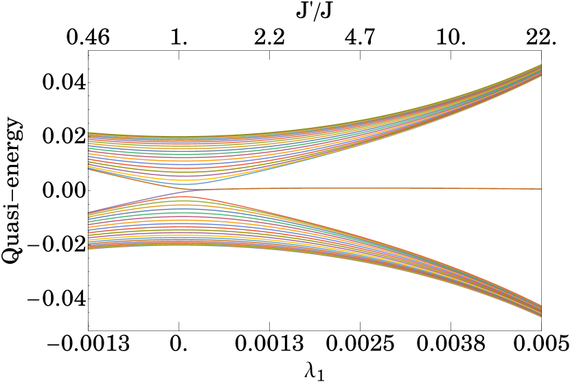
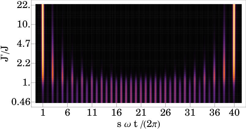
Figure 1: SSH model in the time domain, i.e. a particle bouncing on a periodically oscillating atom mirror, cf. (1). Top panel shows the quasi-energy spectrum related to the $42:1$ resonant manifold ($s=42$) versus $\lambda_{1}$, or equivalently the ratio $J^{\prime}/J$ of the tunneling amplitudes of the effective tight-binding Hamiltonian (3). At two adjacent sites of the tight-binding Hamiltonian (3) a barrier is created, i.e. $a_{s-1}=a_{s}=0$, which allows one to introduce the edge in the system. The barrier is realized by means of an additional modulation of the mirror motion $f(t)=\sum_{k}f_{k}e^{ik\omega t}$ where $f_{k}=\left(10^{-6}\right)k^{2}\omega^{2}\cos(k\pi/42){\rm sinc}^{2}(k\pi/121)$. The zero energy value in the plot has been chosen so that it coincides with the average value of the spectrum presented. Note also that quasi-energy values are given in the gravitational units but they have been multiplied by $10^{5}$. Bottom panel presents one of the two numerical eigenstates corresponding to quasi-energies closest to zero, cf. top panel. In the topological phase, these eigenstates have zero quasi-energy and are linear combinations of the edge states localized at the edge of time. That is, in the laboratory frame, a detector is placed close to the oscillating mirror ($x\approx 0$) and the probability density of clicking of the detector is shown versus time for different values of the ratio $J^{\prime}/J$ of the tunneling amplitudes in (3). This behavior is repeated with the period $2\pi/\omega$. At $s\omega t/(2\pi)=1$ and $s\omega t/(2\pi)=40$ there are edges where the eigenstate localizes if $J^{\prime}/J>1$. The results correspond to $\omega=0.067$, $\lambda=0.06$ in (1) and are obtained within the quantum secular approach [84], see A.

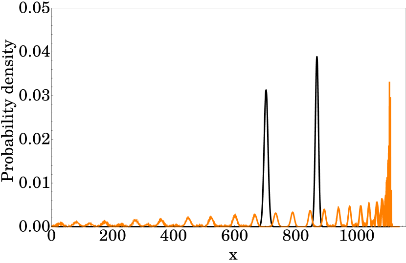
Figure 2: SSH model in the time domain. Black line: probability density of the eigenstate localized at the edge of time as shown in the bottom panel of Fig. 1 for $J^{\prime}/J=22$ but plotted in the configuration space for $s\omega t=39\pi/2$. Orange line presents an example of a bulk eigenstate. The mirror is located at $x\approx 0$ while the classical turning point corresponds to $x=1110$. Note that the crystalline behavior described by Eq. (3) is not observed in the configuration space shown in this plot but in the time domain, see bottom panel of Fig. 1.

3 A time crystal topological insulator

Let us focus on the first energy band of the quantum version of the effective Hamiltonian of Eq. (2) with $V_{2}(\Theta)=0$. The Wannier states $w_{i}(\Theta)$ of the first energy band [85], which are localized in single sites of the periodic potential in Eq. (2), correspond to localized wavepackets $w_{i}(x,t)$ moving along the classical resonant orbit with the period $2\pi/\omega$. For both non-vanishing $V_{0}$ and $V_{1}$, the effective periodic potential describes a Bravais lattice with a two-point basis. Restricting ourselves to the first energy band, i.e. the wavefunction of a particle is expanded as $\psi=\sum_{i=1}^{s}a_{i}w_{i}(\Theta)$, we obtain a tight-binding Hamiltonian

$$H_{\rm eff}\approx-\frac{1}{2}\sum_{i=1}^{s}J_{i}\left(a_{i+1}^{*}a_{i}+c.c.\right),$$ (3)

where $J_{2i}=J^{\prime}$ and $J_{2i-1}=J$, which is identical to the SSH model [86]. The latter describes spinless fermions hopping on a 1D-lattice with staggered hopping amplitudes. Changing the ratio $\lambda_{1}/\lambda$ in (1), allows one to control the ratio $J^{\prime}/J$. This effective Hamiltonian belongs to the BDI class of the periodic table of the topological insulators and superconductors [87] and is characterized by a $\mathbb{Z}$ topological invariant, the winding number $\nu$. For an infinite system with $J^{\prime}>J$ ($J^{\prime}<J$), the system is in a topological (trivial) phase with winding number $\nu=1$ ($\nu=0$). For a finite system, the topological phase exhibits zero energy edge states protected by the topology of the bulk. The SSH model has been experimentally realized in quantum simulators and both the presence of edge states and the winding number have been measured [64, 65, 63]. Let us emphasize that the Wannier states $w_{i}(x,t)$ of Eq. (2) are localized wavepackets of the effective SSH Hamiltonian of Eq. (3). We then discuss how such states allow one to detect the topology of the SSH Hamiltonian.

4 Detection of the topology

The experimental detection of the edge states and the corresponding bulk winding number $\nu$ can be realized in ultra-cold atoms which form a Bose-Einstein condensate (BEC) bouncing on an oscillating atom mirror. The Hamiltonian of Eq. (3) fulfills periodic boundary conditions, i.e. $a_{s+1}=a_{1}$. However, it is possible to introduce an edge in our system by means of a proper modulation of the mirror motion. Indeed, if $f_{k}$’s in the definition of $f(t)$ are suitably chosen, the resulting effective potential $V_{2}(\theta)$ can have a shape of a barrier localized on two adjacent sites of the periodic potential in Eq. (2). Then, the edge is created and two eigenstates can localize exponentially close to it in the topological phase. The corresponding quasi-energy spectrum of the full Floquet Hamiltonian ${\cal H}(t)=H-i\partial_{t}$ is shown in Fig. 1. For $J^{\prime}/J>1$ two degenerate zero-energy levels form which correspond to two eigenstates localized close to the barrier created by the potential $V_{2}(\Theta)$. In the laboratory frame these two eigenstates are related to Floquet states that evolve periodically along the classical resonant orbit. For a detector located close to the orbit, the probability of a detector clicking reveals an edge in time and these two Floquet states localize close to it, as shown in Fig. 1 for increasing values of $J^{\prime}/J$. In Ref. [28] it was proposed how a BEC of non-interacting atoms can be loaded from a trap on a classical resonant orbit: a localized atomic cloud has to be released from a trap at the position of the turning point of the classical resonant orbit above the oscillating mirror. Then, the initial state of the system corresponds to all atoms occupying a single localized state $w_{i}(x,t)$ which evolves along the orbit. An atomic cloud loaded when the edge state is passing close to the turning point remains close to the edge as the edge states do not penetrate much the bulk [63]. How one of the zero-energy eigenstates with the localization close to the edge in time looks like in the configuration space is depicted in Fig. 2 for $s\omega t=39\pi/2$. Measurements of atomic density at different times therefore allow one to confirm the localization properties of the state loaded on the edge.

On the other hand, if an atomic cloud is released in the bulk, then the subsequent time evolution leads to non-zero populations $|a_{i}(t)|^{2}$ of many Wannier wavepackets. Measurement of the atomic density allows one to obtain $|a_{i}(t)|^{2}$ and consequently the winding number which is determined by the mean chiral displacement, i.e. $\nu\approx 2\sum_{i}(i-i_{0})(|a_{2i+1}(t)|^{2}-|a_{2i}(t)|^{2})$ where $i_{0}$ is a number of a cell of the Bravais lattice where the atomic cloud is initially loaded [48, 49, 66]. The relation between $\nu$ and the mean chiral displacement is valid after a long-time evolution when time averaged [66].

5 A time crystal Haldane phase

We now switch from single-particle to many-body systems which are resonantly driven and which can be characterized by non-trivial topology. It is known that a Bose gas in a time-independent spatially periodic lattice with repulsive on-site and nearest-neighbor interactions, described by the following Bose-Hubbard Hamiltonian

$$\hat{H} = -\frac{J}{2}\sum_{i}\left(\hat{a}_{i+1}^{\dagger}\hat{a}_{i}+h.c.\right)+\frac{U}{2}\sum_{i}\hat{n}_{i}(\hat{n}_{i}-1)$$ (5)

$$+V\sum_{i}\hat{n}_{i+1}\hat{n}_{i},$$

can reveal a topological behavior. For large $J$ the Hamiltonian (5) describes superfluid phase of bosons, for large $U$ the Mott insulator (MI) emerges and for large $V$ the density wave (DW) phase is present where translation symmetry of the Hamiltonian (5) is spontaneously broken. However, between the MI phase and the DW phase there is the topological Haldane insulator (HI) phase [88, 89, 90, 91] – or more precisely a bosonic analog of HI in spin-1 chain [56, 57]. As discussed in Ref. [88] this phase breaks a hidden $Z_{2}$ symmetry related to a highly nonlocal string order parameter [92].

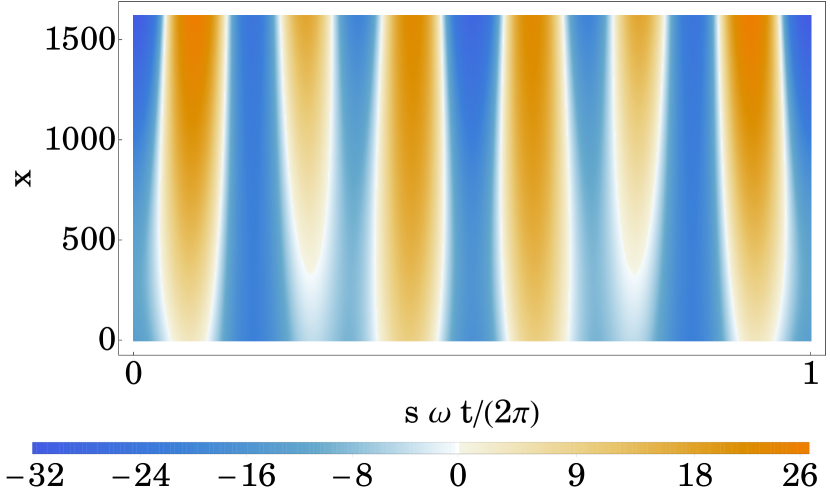
Figure 3: Ultra-cold atoms bouncing on a harmonically oscillating mirror, i.e. $\lambda_{1}=0$ and $f(t)=0$ in (1). Figure shows an example of the dependence of the atomic s-wave scattering length $g_{0}(x,t)\times 10^{-4}$ on a position in space and on time which leads to the effective interactions between bosons described by the on-site and nearest neighbor interaction coefficients $U/J=3$ and $V/J=2.5$. If unit boson filling factor in the effective Bose-Hubbard model is assumed, then the results are related to the HI phase [90]. To realize MI or DW phases, the appropriate $g_{0}(x,t)$ is similar with the amplitude of its oscillations around zero being twice smaller or greater by at least factor 1.5, respectively. The other parameters of the system are the following: $\omega=0.056$, $s=64$ (i.e. $64:1$ resonance), $\lambda=0.14$ and $M=2$ in the expansion $g_{0}=\sum_{m=0}^{M}\alpha(t,m)x^{m}$. The mirror is located at $x=0$ and the turning point of the classical resonant orbit at $x\approx 1600$. The maximal temporal interaction energy per particle is about $1.6\times 10^{4}J$ and thus much smaller than the gap between the first and second quasi-energy bands of the corresponding single-particle problem which is $1.1\times 10^{5}J$ where $J=5.5\times 10^{-8}$. The results are obtained within the quantum secular approach [84], see A.

To realize a resonantly driven system that, in the time-periodic Wannier-like modes $w_{i}(x,t)$ of Eq. (2), is effectively described by the Hamiltonian of (5), we again consider ultra-cold bosons bouncing on an oscillating mirror. We assume that the single-particle Hamiltonian corresponds to Eq. (1) with $\lambda_{1}=0$ and $f(t)=0$. For the resonant driving described above, we may restrict to the first energy band of the effective Hamiltonian (2) that leads to the tight-binding model (3). In the many-body case when we restrict to the Hilbert subspace spanned by Fock states $|n_{1},\dots,n_{s}\rangle$, where $n_{i}$’s denote numbers of bosons occupying Wannier wavepackets $w_{i}(x,t)$, we obtain the effective many-body Hamiltonian which resembles (5) but with the interaction terms ${1/2}\sum_{i,j=1}^{s}U_{ij}\hat{a}_{i}^{\dagger}\hat{a}_{j}^{\dagger}\hat{a}_{j}\hat{a}_{i}$ where $U_{ij}=2\int_{0}^{2\pi/\omega}dt\int_{0}^{\infty}dxg_{0}|w_{i}|^{2}|w_{j}|^{2}$ for $i\neq j$ and similar $U_{ii}$ but twice smaller [35] (see A). The effective interaction coefficients $U_{ij}$ depend on the atomic s-wave scattering length $g_{0}$, shapes of $|w_{i}(x,t)|^{2}$ and how densities of different Wannier wavepackets overlap in the course of time evolution on the classical resonant orbit. Despite the fact that the original interactions between ultra-cold atoms are contact, the effective interactions can be long-range [93, 35, 42]. Moreover, they can be controlled by changing the s-wave scattering length in space and periodically in time by means of a Feshbach resonance, i.e. $g_{0}=g_{0}(x,t)$. Indeed, if the applied magnetic field results in appropriate oscillations of the scattering length around zero, nearly arbitrary effective long-range interactions can be created. In order to perform a systematic analysis of the control of $U_{ij}$, we assume that $g_{0}(x,t)=\sum_{m=0}^{M}\alpha(t,m)x^{m}$ and write the interaction coefficients in the form $U_{ij}=\sum_{m=0}^{M}\int_{0}^{2\pi/\omega}dt\alpha(t,m)u_{ij}(t,m)$. To find a suitable $\alpha(t,m)$ one can apply the singular value decomposition of the matrix $u_{ij}(t,m)$ where $(i,j)$ and $(t,m)$ are treated as indices of rows and columns, respectively [40]. Left singular vectors tell us which sets of interaction coefficients $U_{ij}$ can be realized, while the corresponding right singular vectors give the recipes for $\alpha(t,m)$ and consequently for $g_{0}(x,t)$. In Fig. 3 we show an example of $g_{0}(x,t)$ corresponding to $U_{ii}=U$, $U_{ij}=V$ for $|i-j|=1$ and $U_{ij}=0$ when $|i-j|>1$ where $U/J=3$ and $V/J=2.5$. These values are related to the Haldane insulator phase if the unit mean boson filling factor is assumed [90]. In order to realize topologically trivial MI or DW phases, the corresponding $g_{0}(x,t)/J$ may take a similar form with the amplitude of its oscillations around zero being about twice smaller for MI or at least a factor 1.5 greater for the DW phase. For example, for the parameters of Ref. [28], if one wants to modulate the scattering length around zero value with the amplitude of two Bohr radius, the magnetic field has to change with the speed 0.5G/ms — well within the experimental reach [94].

It is quite straightforward to prepare initially all bosons in a single Wannier state $w_{i}(x,t)$ by releasing atomic cloud from a trap at the classical turning point above the mirror [28]. However, the preparation of the system in lowest quasi-energy state within the resonant subspace, i.e. in the ground state of (5) is not easy. An open question remains whether the time-evolution after a quench of a localized initial state can reveal the topology of the Haldane Insulating phase. This problem is beyond the scope of the present paper.

Finally let us analyse whether the resonant driving does not heat the system considerably. Consider first a single particle problem. While a harmonic oscillator can absorb continuously energy when resonantly driven, we consider a model with nonlinear resonances — a particle bouncing resonantly on an oscillating mirror [83]. For such a system its period of motion depends on energy, so when a particle absorbs energy, its period changes and a particle gets out of the resonance. The resonant transfer of energy stops [82]. The non-linear resonances are related to the presence of elliptical islands in the classical phase space [82], see Fig. 4 in A. Floquet states located inside the islands are strongly localized [83]. Their coupling to other states localized outside the islands, for any type of weak additional coupling is exponentially small precisely due to the semiclassical localization. Such a coupling may be provided by e.g. weak interactions among the particles that require a consideration of necessarily enlarged $2N$-dimensional phase space. Such an additional coupling of a subspace of Floquet states localized in the islands to the complementary Hilbert subspace can be tested within the mean field approach as an exact many-body analysis is obviously beyond the current possibilities. A careful mean-field analysis performed in [28] indicates that, on the relevant experimentally time scale, such a coupling (and the resulting heating) is negligible also if typical experimental imperfections are taken into account. Thus the relevant physics takes place in the resonant subspace of Floquet states localized in the phase space and are immune to heating, at least for a time scale much longer than the experimentally relevant one [28], without any disorder present. If interactions are sufficiently weak then the physics may be described within the lowest band of the Bose-Hubbard model constructed in the paper.

6 Discussion

We have shown how one can construct topological insulators in the time domain. To this end we considered bosons bouncing on the periodically oscillating atom mirror, topological phases are obtained by an appropriate tuning the shape of the oscillations. We presented explicit schemes for the realization of the effective SSH and the extended Bose-Hubbard Hamiltonians which possess topological behavior in the time domain. In the case of the topological SSH, we proposed a detection method of the topological properties in time with state-of-the-art techniques [28]. In the case of the Haldane insulator, the experimental detection of the topological phase remains a challenge.

Note added: After the submission of the present manuscript we learned about the work on a similar topic but in photonic materials [95].

Appendix A

In this Appendix we present the derivation of the effective Hamiltonians used in the paper. We also provide a detailed explanation of the emergence of crystalline structures in the time domain in the course of dynamical evolution of resonantly driven systems.

A.1 Classical effective Hamiltonian

We consider a single atom bouncing on an oscillating atom mirror in the presence of the gravitational force. The Hamiltonian of the system, in the frame oscillating with the mirror [83] (then the mirror is fixed) and in the gravitational units, reads

$$H = H_{0}+H_{1},$$ (6)

$$H_{0} = \frac{p^{2}}{2}+x,$$ (7)

$$H_{1} = x\left[\lambda\cos(s\omega t)+\lambda_{1}\cos(s\omega t/2)+f(t)\right],$$ (8)

where $H_{1}$ describes the oscillation of the mirror composed of two harmonics. $s$ is an integer number and

$$f(t)=f(t+2\pi/\omega)=\sum_{k}f_{k}e^{ik\omega t}.$$ (9)

We assume $x\geq 0$ with the mirror located at $x=0$. At first glance the system does not have anything in common with a solid state-like behavior. In order to demonstrate that for a resonant driving of the particle motion, the system behaves like a condensed matter system (and in particular may possess topological properties) let us begin with the classical description and apply the secular approximation [82, 83].

First we apply the canonical transformation from the Cartesian position $x$ and momentum $p$ to the so-called action-angle variables. Then, the unperturbed Hamiltonian depends on the new momentum (action) only [83],

$$H_{0}=\frac{1}{2}(3\pi I)^{2/3},$$ (10)

and the solution of the unperturbed particle motion is straightforward. That is, the action is a constant of motion, $I=$const, and the conjugate position variable (the angle) evolves linearly in time, $\theta(t)=\Omega(I)\;t+\theta(0)$, where $\Omega(I)=dH_{0}(I)/dI$ is the frequency of periodic evolution of a particle. The perturbation part of the Hamiltonian, in the new canonically conjugate variables, reads

$$H_{1} = \left(\sum_{n}h_{n}(I)e^{in\theta}\right)\left(\sum_{m}F_{m}e^{im\omega t}\right),$$ (11)

where $h_{0}=\left(\frac{\pi I}{\sqrt{3}}\right)^{2/3}$ and $h_{n}=\frac{(-1)^{n+1}}{n^{2}}\left(\frac{3I}{\pi^{2}}\right)^{2/3}$ for $n\neq 0$, and $F_{m}$ are Fourier components of the time-periodic function in (8).

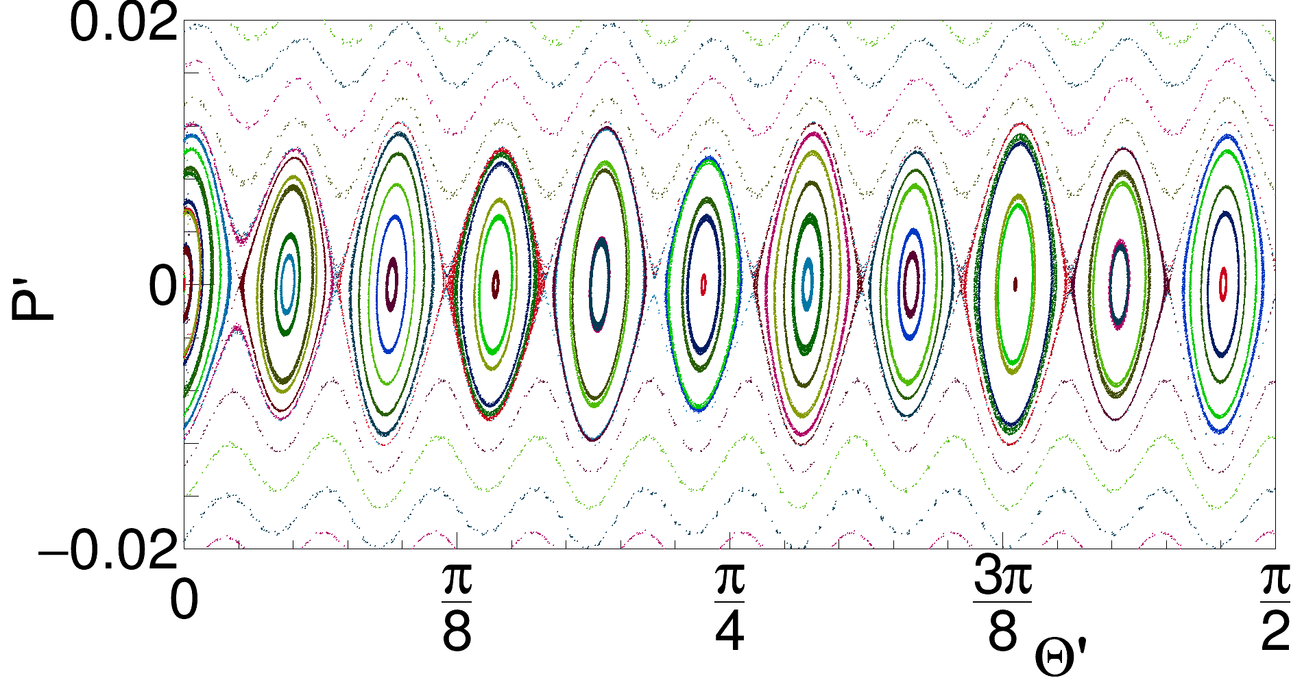
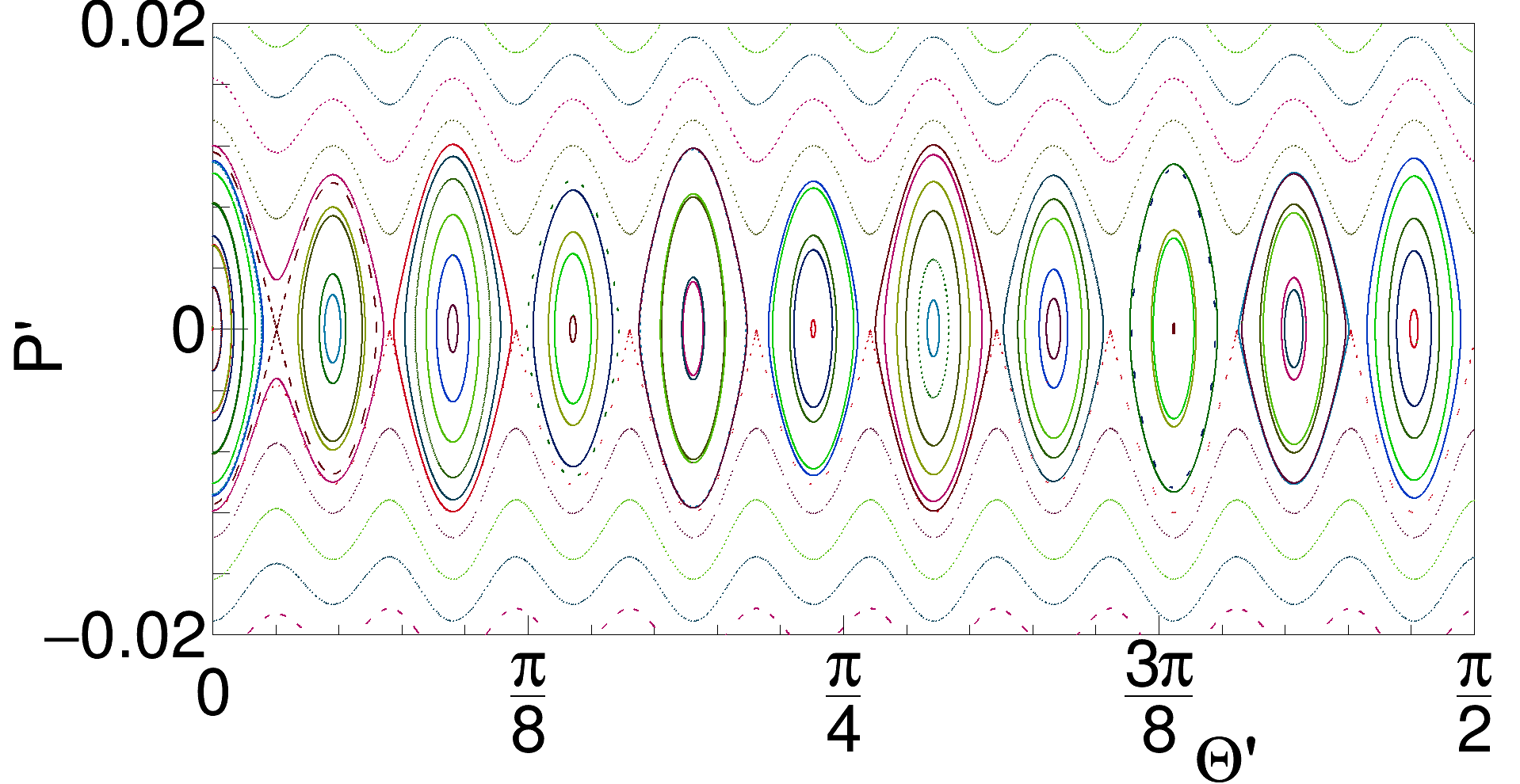
Figure 4: Comparison of the exact stroboscopic picture (top panel) of the system phase space with the phase space portrait (bottom panel) obtained with the help of the effective Hamiltonian (LABEL:sshHs). The parameters of the system are the same as those used in the paper in Figs. 1-2, i.e. $s=42$, $\omega=0.067$, $\lambda=0.06$, $\lambda_{1}=0.005$ and $f_{k}=\left(10^{-6}\right)k^{2}\omega^{2}\cos(k\pi/42){\rm sinc}^{2}(k\pi/121)$. Scaled variables have been used in the plot, i.e. $P^{\prime}=P/I_{0}$ and $\Theta^{\prime}=\Theta$. Note that for the sake of clarity we show only a quarter of the full $2\pi$ range of $\Theta^{\prime}$.

Next, we assume that a particle is resonantly driven, that is the frequency $\omega$ is equal to the frequency of the unperturbed motion, i.e. $\omega=\Omega(I_{0})$ where $I_{0}$ is the resonant value of the action. We are interested in initial conditions of a particle where the action $I\approx I_{0}$. Then, it is convenient to perform another canonical transformation to the moving frame, associated with the motion along the resonant orbit [82],

$$\Theta = \theta-\omega t,$$ (12)

$${\cal I} = I.$$ (13)

In that frame, the Hamiltonian of the system takes the form

$$H = \frac{1}{2}\left(3\pi{\cal I}\right)^{2/3}-\omega{\cal I}+\sum_{n,m}h_{n}({\cal I})F_{m}e^{in\Theta}e^{i(n+m)\omega t}.$$ (14)

Now, if we are interested in the motion close to the resonant orbit, i.e. when ${\cal I}\approx I_{0}$, both $\cal I$ and $\Theta$ are changing slowly if the perturbation is weak. The only fast variable is time and we can significantly simplify the description by averaging the Hamiltonian (LABEL:fullmovHs) over time [82] that results in

$$H_{\rm eff} = \frac{P^{2}}{2m_{\rm eff}}-V_{0}\cos(s\Theta)-V_{1}\cos(s\Theta/2)-V_{2}(\Theta),$$ (16)

which is the effective Hamiltonian (2) in the paper. In (LABEL:sshHs)

$$m_{\rm eff} = -\frac{\pi^{2}}{\omega^{4}},$$ (18)

$$V_{0} = \lambda\frac{(-1)^{s}}{s^{2}\omega^{2}},$$ (19)

$$V_{1} = \lambda_{1}\frac{4(-1)^{s/2}}{s^{2}\omega^{2}},$$ (20)

$$V_{2}(\Theta) = \sum_{n}\frac{(-1)^{n}}{n^{2}\omega^{2}}f_{-n}e^{in\Theta},$$ (21)

and we have performed Taylor expansion around $P={\cal I}-I_{0}\approx 0$. The validity of the effective Hamiltonian (LABEL:sshHs) can be easily tested by comparing the exact stroboscopic picture of the system phase space with the phase space portrait generated by the Hamiltonian (LABEL:sshHs). It is done in Fig. 4 which demonstrates that the secular approach captures quantitatively the dynamics of the system.

A.2 Quantum effective Hamiltonian

So far we have performed the classical analysis. In order to switch to the effective quantum description we can either perform a quantization of the classical effective Hamiltonian (LABEL:sshHs) or apply a quantum version of the secular approximation for the Hamiltonian (6) [84]. Let us first discuss the former approach. Classical equations of motion possess the scaling symmetry which implies that by a proper rescaling of the parameters and the dynamical variables of the system we obtain the same behavior as presented in Fig. 4 but around arbitrary value of $I_{0}$ [83]. That is, when we redefine $\omega^{\prime}=I_{0}^{-1/3}\omega$ and $\lambda^{\prime}=\lambda$ we can use the results presented in Fig. 4 if we rescale $p^{\prime}=I_{0}^{1/3}p$, $x^{\prime}=I_{0}^{2/3}x$ and $t^{\prime}=I_{0}^{1/3}t$. In the quantum description the scaling symmetry is broken because the Planck constant sets a scale in the phase space,

$$[x,p]=i\quad\Rightarrow\quad[x^{\prime},p^{\prime}]=\frac{i}{I_{0}}.$$ (22)

From (22) we see that $1/I_{0}$ plays a role of the effective Planck constant. Thus, for $I_{0}\gg 1$, quantization of the effective Hamiltonian (LABEL:sshHs), obtained in the action-angle variables, i.e. when $P\rightarrow-i\frac{\partial}{\partial\Theta}$, provides perfect quantum description of the resonant behavior of the system. The same quantum results can be obtained by applying the quantum secular approach [84] which yields

$$\langle n^{\prime}|H_{\rm eff}|n\rangle=\left(E_{n}-n\omega\right)\delta_{nn^{\prime}}+\langle n^{\prime}|x|n\rangle F_{n-n^{\prime}},$$ (23)

where $|n\rangle$’s are eigenstates of the unperturbed system and $2^{1/3}E_{n}$ are zeros of the Airy function [83] and $F_{n}$ are Fourier components of the time periodic function in (8). Equation (23) has been obtained by switching to the moving frame, with the help of the unitary transformation $\hat{U}=e^{i\hat{n}\omega t}$, and by averaging the resulting Hamiltonian over time [84].

A.3 Crystalline structure in time

For $f(t)=0$, and consequently for $V_{2}(\Theta)=0$ in (LABEL:sshHs), and for $s\gg 1$, corresponding classically to the $s:1$ resonance between the motion of the particle in the gravitational field and mirror oscillations, the effective Hamiltonian becomes identical to a solid state system with an electron moving in a periodic potential in space with periodic boundary conditions. In the quantum description, eigenstates of (LABEL:sshHs) are Bloch waves $e^{ik\Theta}u_{n}(\Theta)$ where $k$ is a quasi-momentum, $n$ denotes a number of an energy band and $u_{n}(\Theta+2\pi/s)=u_{n}(\Theta)$. Such a crystalline structure that we observe in the frame moving along the resonant orbit is reproduced in the time domain when we return to the laboratory frame [35, 36]. Indeed, when we locate a detector in the laboratory frame close to the resonant orbit (i.e. at a space point where $I\approx I_{0}$ and $\theta=$const), probability for clicking of the detector as a function of time reproduces periodic behavior versus $\Theta$ that we obtain in the moving frame with the help of the effective Hamiltonian (LABEL:sshHs). This is the crucial property of the system we consider here and it is related to the fact that the transformation between the laboratory frame and the moving frame is linear in time, see (12). Thus, for $\theta=$const we obtain the same behavior in time as versus $\Theta$ in the moving frame, $e^{ik(\theta-\omega t)}u_{n}(\theta-\omega t)=e^{ik\Theta}u_{n}(\Theta)$. We would like to stress that such a crystalline structure in time is not a result of the presence of any potential periodic in space. It emerges in the dynamics of the system due to the resonant driving and a high resonance order $s$.

A.4 Tight-binding approximation

Assume that $V_{2}(\Theta)=0$ in (LABEL:sshHs). If we are interested in the first energy band of the effective Hamiltonian (LABEL:sshHs), the description of the system can still be simplified. Suppose that $w_{i}(\Theta)$ are Wannier functions corresponding to the first energy band of (LABEL:sshHs). Then, expanding the wavefunction of a particle in the Wannier function basis, $\psi(\Theta)=\sum_{i=1}^{s}a_{i}w_{i}(\Theta)$, we obtain the tight-binding Hamiltonian, cf. (3) in the paper,

$$H_{\rm eff}\approx-\frac{1}{2}\sum_{i=1}^{s}J_{i}\left(a_{i+1}^{*}a_{i}+c.c.\right),$$ (24)

where tunneling amplitudes $J_{i}=-2\int_{0}^{2\pi}d\Theta w_{i+1}^{*}H_{\rm eff}w_{i}$ describe tunneling of a particle between neighbouring sites of the potential in (LABEL:sshHs). There are also longer range tunnelings but they are orders of magnitude weaker for the parameters we consider in the paper. For $\lambda_{1}\neq 0$ when $J=J_{2i-1}$, $J^{\prime}=J_{2i}$ and $J\neq J^{\prime}$, the Hamiltonian (24) describes a particle in a Bravais lattice with a two-point basis. Actually it is the SSH model [86] which can possess topological properties.

The tight-binding Hamiltonian (24) describes a particle in the Wannier function basis. In the laboratory frame this is the basis of localized wavepackets which evolve periodically along the resonant orbit, i.e. in the Cartesian coordinate frame $w_{i}(x,t+2\pi/\omega)=w_{i}(x,t)$. It shows that condensed matter physics in the time domain we consider here can be described by a solid state model but in the time-periodic basis.

A.5 Many-body problem

Having introduced a tight-binding model for a single particle problem, we can easily switch to the many-body case. Indeed, assume that we have $N$ bosons which interact via Dirac-delta potential $g_{0}\delta(x)$ and we restrict to the resonant Hilbert subspace of the system. That is, we restrict to the Hilbert subspace spanned by Fock states $|n_{1},\dots,n_{s}\rangle$ where $n_{i}$ denotes a number of particles that occupy a Wannier state $w_{i}(x,t)$. Then, the effective many-body Hamiltonian takes the form of the Bose-Hubbard model [35],

$$\hat{H} = -\frac{1}{2}\sum_{i}\left(J_{i}\hat{a}_{i+1}^{\dagger}\hat{a}_{i}+h.c.\right)+\frac{1}{2}\sum_{i,j=1}^{s}U_{ij}\hat{a}_{i}^{\dagger}\hat{a}_{j}^{\dagger}\hat{a}_{j}\hat{a}_{i},$$ (25)

where $\hat{a}_{i}$ are standard bosonic annihilation operators and

$$U_{ij} = 2\int\limits_{0}^{2\pi/\omega}dt\int\limits_{0}^{\infty}dx\;g_{0}\;|w_{i}(x,t)|^{2}|w_{j}(x,t)|^{2},\quad{\rm for}\;i\neq j,$$ (27)

$$U_{ii} = \int\limits_{0}^{2\pi/\omega}dt\int\limits_{0}^{\infty}dx\;g_{0}\;|w_{i}(x,t)|^{4},$$ (28)

are coefficients which describe interactions between particles. If $n_{i}$ bosons occupy a given localized Wannier-like wavepacket $w_{i}(x,t)$ they interact that is related to the on-site interactions in (LABEL:bhhs). However, bosons occupying different localized wavepackets $w_{i}(x,t)$ and $w_{j}(x,t)$ also interact because in the course of time evolution along the resonant orbit the wavepackets pass each other. That leads to effective long-range interactions in the Bose-Hubbard Hamiltonian (LABEL:bhhs). Moreover, the long-range interaction can be engineered if the s-wave scattering length of atoms is periodically modulated in time and depends on a position in space, i.e. $g_{0}=g_{0}(x,t)$.

The effective Bose-Hubbard Hamiltonian is valid if the maximal interaction energy per particle is much smaller than the energy gap $\Delta E$ between the first and second energy bands of the single-particle Hamiltonian (LABEL:sshHs). In the paper we assume that the interaction energy is larger than the width of the first energy band (which is of the order of $J$) but much smaller than $\Delta E$. There is no problem to fulfill this condition because $\Delta E\gg J$.

References

References

- [1] Wilczek F 2012 Phys. Rev. Lett. 109(16) 160401 URL http://link.aps.org/doi/10.1103/PhysRevLett.109.160401
- [2] Bruno P 2013 Phys. Rev. Lett. 111(7) 070402 URL http://link.aps.org/doi/10.1103/PhysRevLett.111.070402
- [3] Watanabe H and Oshikawa M 2015 Phys. Rev. Lett. 114(25) 251603 URL http://link.aps.org/doi/10.1103/PhysRevLett.114.251603
- [4] Syrwid A, Zakrzewski J and Sacha K 2017 Phys. Rev. Lett. 119(25) 250602 URL https://link.aps.org/doi/10.1103/PhysRevLett.119.250602
- [5] Sacha K and Zakrzewski J 2018 Rep. Prog. Phys. 81 016401 URL https://doi.org/10.1088/1361-6633/aa8b38
- [6] Shapere A and Wilczek F 2012 Phys. Rev. Lett. 109(16) 160402 URL http://link.aps.org/doi/10.1103/PhysRevLett.109.160402
- [7] Ghosh S 2014 Physica A: Statistical Mechanics and its Applications 407 245 – 251 ISSN 0378-4371 URL http://www.sciencedirect.com/science/article/pii/S0378437114003161
- [8] Yao N Y, Nayak C, Balents L and Zaletel M P 2018 ArXiv e-prints (Preprint 1801.02628)
- [9] Das P, Pan S, Ghosh S and Pal P 2018 Phys. Rev. D 98(2) 024004 URL https://link.aps.org/doi/10.1103/PhysRevD.98.024004
- [10] Alvarez P, Canfora F, Dimakis N and Paliathanasis A 2017 Physics Letters B 773 401 – 407 ISSN 0370-2693 URL http://www.sciencedirect.com/science/article/pii/S0370269317306950
- [11] Avilés L, Canfora F, Dimakis N and Hidalgo D 2017 Phys. Rev. D 96(12) 125005 URL https://link.aps.org/doi/10.1103/PhysRevD.96.125005
- [12] Sacha K 2015 Phys. Rev. A 91(3) 033617 URL http://link.aps.org/doi/10.1103/PhysRevA.91.033617
- [13] Khemani V, Lazarides A, Moessner R and Sondhi S L 2016 Phys. Rev. Lett. 116(25) 250401 URL http://link.aps.org/doi/10.1103/PhysRevLett.116.250401
- [14] Else D V, Bauer B and Nayak C 2016 Phys. Rev. Lett. 117(9) 090402 URL http://link.aps.org/doi/10.1103/PhysRevLett.117.090402
- [15] Yao N Y, Potter A C, Potirniche I D and Vishwanath A 2017 Phys. Rev. Lett. 118(3) 030401 URL http://link.aps.org/doi/10.1103/PhysRevLett.118.030401
- [16] Lazarides A and Moessner R 2017 Phys. Rev. B 95(19) 195135 URL https://link.aps.org/doi/10.1103/PhysRevB.95.195135
- [17] Russomanno A, Iemini F, Dalmonte M and Fazio R 2017 Phys. Rev. B 95(21) 214307 URL https://link.aps.org/doi/10.1103/PhysRevB.95.214307
- [18] Zeng T S and Sheng D N 2017 Phys. Rev. B 96(9) 094202 URL https://link.aps.org/doi/10.1103/PhysRevB.96.094202
- [19] Nakatsugawa K, Fujii T and Tanda S 2017 Phys. Rev. B 96(9) 094308 URL https://link.aps.org/doi/10.1103/PhysRevB.96.094308
- [20] Ho W W, Choi S, Lukin M D and Abanin D A 2017 Phys. Rev. Lett. 119(1) 010602 URL https://link.aps.org/doi/10.1103/PhysRevLett.119.010602
- [21] Huang B, Wu Y H and Liu W V 2018 Phys. Rev. Lett. 120(11) 110603 URL https://link.aps.org/doi/10.1103/PhysRevLett.120.110603
- [22] Gong Z, Hamazaki R and Ueda M 2018 Phys. Rev. Lett. 120(4) 040404 URL https://link.aps.org/doi/10.1103/PhysRevLett.120.040404
- [23] Wang R R W, Xing B, Carlo G G and Poletti D 2018 Phys. Rev. E 97(2) 020202 URL https://link.aps.org/doi/10.1103/PhysRevE.97.020202
- [24] Bomantara R W and Gong J 2018 Phys. Rev. Lett. 120(23) 230405 URL https://link.aps.org/doi/10.1103/PhysRevLett.120.230405
- [25] Autti S, Eltsov V B and Volovik G E 2018 Phys. Rev. Lett. 120(21) 215301 URL https://link.aps.org/doi/10.1103/PhysRevLett.120.215301
- [26] Kosior A and Sacha K 2018 Phys. Rev. A 97(5) 053621 URL https://link.aps.org/doi/10.1103/PhysRevA.97.053621
- [27] Mizuta K, Takasan K, Nakagawa M and Kawakami N 2018 ArXiv e-prints (Preprint 1804.01291)
- [28] Giergiel K, Kosior A, Hannaford P and Sacha K 2018 Phys. Rev. A 98(1) 013613 URL https://link.aps.org/doi/10.1103/PhysRevA.98.013613
- [29] Kosior A, Syrwid A and Sacha K 2018 Phys. Rev. A 98(2) 023612 URL https://link.aps.org/doi/10.1103/PhysRevA.98.023612
- [30] Zhang J, Hess P W, Kyprianidis A, Becker P, Lee A, Smith J, Pagano G, Potirniche I D, Potter A C, Vishwanath A, Yao N Y and Monroe C 2017 Nature 543 217–220 ISSN 0028-0836 letter URL http://dx.doi.org/10.1038/nature21413
- [31] Choi S, Choi J, Landig R, Kucsko G, Zhou H, Isoya J, Jelezko F, Onoda S, Sumiya H, Khemani V, von Keyserlingk C, Yao N Y, Demler E and Lukin M D 2017 Nature 543 221–225 ISSN 0028-0836 letter URL http://dx.doi.org/10.1038/nature21426
- [32] Pal S, Nishad N, Mahesh T S and Sreejith G J 2018 Phys. Rev. Lett. 120(18) 180602 URL https://link.aps.org/doi/10.1103/PhysRevLett.120.180602
- [33] Rovny J, Blum R L and Barrett S E 2018 Phys. Rev. Lett. 120(18) 180603 URL https://link.aps.org/doi/10.1103/PhysRevLett.120.180603
- [34] Rovny J, Blum R L and Barrett S E 2018 Phys. Rev. B 97(18) 184301 URL https://link.aps.org/doi/10.1103/PhysRevB.97.184301
- [35] Sacha K 2015 Sci. Rep. 5 10787 URL https://www.nature.com/articles/srep10787
- [36] Sacha K and Delande D 2016 Phys. Rev. A 94(2) 023633 URL http://link.aps.org/doi/10.1103/PhysRevA.94.023633
- [37] Giergiel K and Sacha K 2017 Phys. Rev. A 95(6) 063402 URL https://link.aps.org/doi/10.1103/PhysRevA.95.063402
- [38] Mierzejewski M, Giergiel K and Sacha K 2017 Phys. Rev. B 96(14) 140201 URL https://link.aps.org/doi/10.1103/PhysRevB.96.140201
- [39] Delande D, Morales-Molina L and Sacha K 2017 Phys. Rev. Lett. 119(23) 230404 URL https://link.aps.org/doi/10.1103/PhysRevLett.119.230404
- [40] Giergiel K, Miroszewski A and Sacha K 2018 Phys. Rev. Lett. 120(14) 140401 URL https://link.aps.org/doi/10.1103/PhysRevLett.120.140401
- [41] Guo L, Marthaler M and Schön G 2013 Phys. Rev. Lett. 111(20) 205303 URL https://link.aps.org/doi/10.1103/PhysRevLett.111.205303
- [42] Guo L and Marthaler M 2016 New J. Phys. 18 023006 URL http://stacks.iop.org/1367-2630/18/i=2/a=023006
- [43] Guo L, Liu M and Marthaler M 2016 Phys. Rev. A 93(5) 053616 URL https://link.aps.org/doi/10.1103/PhysRevA.93.053616
- [44] Liang P, Marthaler M and Lingzhen G 2018 New J. Phys. 20 023043 ISSN 1367-2630 URL http://stacks.iop.org/1367-2630/20/i=2/a=023043
- [45] Senthil T 2015 Annual Review of Condensed Matter Physics 6 299 URL https://doi.org/10.1146%2Fannurev-conmatphys-031214-014740
- [46] Przysiȩżna A, Dutta O and Zakrzewski J 2015 New J. Phys. 17 013018 URL http://stacks.iop.org/1367-2630/17/i=1/a=013018
- [47] Biedroń K, Dutta O and Zakrzewski J 2016 Phys. Rev. A 93(3) 033631 URL https://link.aps.org/doi/10.1103/PhysRevA.93.033631
- [48] Cardano Filippo, D’Errico Alessio, Dauphin Alexandre, Maffei Maria, Piccirillo Bruno, de Lisio Corrado, De Filippis Giulio, Cataudella Vittorio, Santamato Enrico, Marrucci Lorenzo, Lewenstein Maciej and Massignan Pietro 2017 Nature Communications 8 15516 URL https://www.nature.com/articles/ncomms15516#supplementary-information
- [49] Maffei M, Dauphin A, Cardano F, Lewenstein M and Massignan P 2018 New J. Phys. 20 013023 URL http://stacks.iop.org/1367-2630/20/i=1/a=013023
- [50] Kitagawa T, Berg E, Rudner M and Demler E 2010 Phys. Rev. B 82(23) 235114 URL https://link.aps.org/doi/10.1103/PhysRevB.82.235114
- [51] von Keyserlingk C W and Sondhi S L 2016 Phys. Rev. B 93(24) 245145 URL http://link.aps.org/doi/10.1103/PhysRevB.93.245145
- [52] Else D V and Nayak C 2016 Phys. Rev. B 93(20) 201103
- [53] Potter A C, Morimoto T and Vishwanath A 2016 Phys. Rev. X 6(4) 041001 URL http://link.aps.org/doi/10.1103/PhysRevX.6.041001
- [54] Roy R and Harper F 2016 Phys. Rev. B 94(12) 125105 URL http://link.aps.org/doi/10.1103/PhysRevB.94.125105
- [55] Xu S and Wu C 2018 Phys. Rev. Lett. 120(9) 096401 URL https://link.aps.org/doi/10.1103/PhysRevLett.120.096401
- [56] Haldane F D M 1983 Phys. Lett. A 93 464
- [57] Haldane F D M 1983 Phys. Rev. Lett. 50 1153
- [58] Hasan M Z and Kane C L 2010 Rev. Mod. Phys. 82(4) 3045–3067 URL https://link.aps.org/doi/10.1103/RevModPhys.82.3045
- [59] Goldman N, Juzeliunas G, Öhberg P and Spielman I B 2014 Rep. Prog. Phys. 77 126401 URL http://stacks.iop.org/0034-4885/77/i=12/a=126401
- [60] Ozawa T, Price H M, Amo A, Goldman N, Hafezi M, Lu L, Rechtsman M, Schuster D, Simon J, Zilberberg O and Carusotto I 2018 arXiv:1802.04173
- [61] Lewenstein M, Sanpera A and Ahufinger V 2007 Ultracold atoms in Optical Lattices: simulating quantum many body physics (Oxford University Press, Oxford)
- [62] Kitagawa T, Broome M a, Fedrizzi A, Rudner M S, Berg E, Kassal I, Aspuru-Guzik A, Demler E and White A G 2012 Nat. Comm. 3 882 ISSN 2041-1723 URL http://www.nature.com/doifinder/10.1038/ncomms1872
- [63] Meier Eric J, An Fangzhao Alex and Gadway Bryce 2016 Nature Communications 7 13986 URL https://www.nature.com/articles/ncomms13986#supplementary-information
- [64] Atala M, Aidelsburger M, Barreiro J T, Abanin D, Kitagawa T, Demler E and Bloch I 2013 Nature Physics 9 79 URL https://doi.org/10.1038%2Fnphys2790
- [65] St-Jean P, Goblot V, Galopin E, Lemaître A, Ozawa T, Gratiet L L, Sagnes I, Bloch J and Amo A 2017 Nature Photonics 11 651 URL https://doi.org/10.1038%2Fs41566-017-0006-2
- [66] Meier E J, An F A, Dauphin A, Maffei M, Massignan P, Hughes T L and Gadway B 2018 ArXiv e-prints (Preprint 1802.02109)
- [67] de Léséleuc S, Lienhard V, Scholl P, Barredo D, Weber S, Lang N, Büchler H P, Lahaye T and Browaeys A 2018 arXiv e-prints arXiv:1810.13286 (Preprint 1810.13286)
- [68] Aidelsburger M, Lohse M, Schweizer C, Atala M, Barreiro J T, Nascimbène S, Cooper N R, Bloch I and Goldman N 2015 Nat. Phys. 11 162 ISSN 17452481 (Preprint 1407.4205) URL http://arxiv.org/abs/1407.4205
- [69] Stuhl B K, Lu H I, Aycock L M, Genkina D and Spielman I B 2015 Science 349 1514–1518 ISSN 0036-8075 URL http://www.sciencemag.org/cgi/doi/10.1126/science.aaa8515
- [70] Tarnowski M, Nur Ünal F, Fläschner N, Rem B S, Eckardt A, Sengstock K and Weitenberg C 2017 ArXiv e-prints (Preprint 1709.01046)
- [71] Lohse M, Schweizer C, Price H M, Zilberberg O and Bloch I 2018 Nature 553 55
- [72] Zilberberg O, Huang S, Guglielmon J, Wang M, Chen K P, Kraus Y E and Rechtsman M C 2018 Nature 553 59
- [73] Steane A, Szriftgiser P, Desbiolles P and Dalibard J 1995 Phys. Rev. Lett. 74(25) 4972–4975 URL http://link.aps.org/doi/10.1103/PhysRevLett.74.4972
- [74] Roach T M, Abele H, Boshier M G, Grossman H L, Zetie K P and Hinds E A 1995 Phys. Rev. Lett. 75(4) 629–632 URL https://link.aps.org/doi/10.1103/PhysRevLett.75.629
- [75] Sidorov A I, McLean R J, Rowlands W J, Lau D C, Murphy J E, Walkiewicz M, Opat G I and Hannaford P 1996 Quantum and Semiclassical Optics: Journal of the European Optical Society Part B 8 713 URL http://stacks.iop.org/1355-5111/8/i=3/a=030
- [76] Westbrook N, Westbrook C I, Landragin A, Labeyrie G, Cognet L, Savalli V, Horvath G, Aspect A, Hendel C, Moelmer K, Courtois J Y, Phillips W D, Kaiser R and Bagnato V 1998 Physica Scripta 1998 7 URL http://stacks.iop.org/1402-4896/1998/i=T78/a=001
- [77] Lau D C, Sidorov A I, Opat G I, McLean R J, Rowlands W J and Hannaford P 1999 Eur. Phys. J. D 5 193–199 URL https://doi.org/10.1007/s100530050244
- [78] Bongs K, Burger S, Birkl G, Sengstock K, Ertmer W, Rza̧żewski K, Sanpera A and Lewenstein M 1999 Phys. Rev. Lett. 83(18) 3577–3580 URL https://link.aps.org/doi/10.1103/PhysRevLett.83.3577
- [79] Sidorov A, McLean R, Scharnberg F, Gough D, Davis T, Sexton B, Opat G and Hannaford P 2002 Acta Phys. Pol. B 33(8) 2137
- [80] Fiutowski J, Bartoszek-Bober D, Dohnalik T and Kawalec T 2013 Opt. Commun. 297 59
- [81] Kawalec T, Bartoszek-Bober D, Panaś R, Fiutowski J, Pławecka A and Rubahn H G 2014 Opt. Lett. 39 2932–2935 URL http://ol.osa.org/abstract.cfm?URI=ol-39-10-2932
- [82] Lichtenberg A and Lieberman M 1992 Regular and chaotic dynamics Applied mathematical sciences (Springer-Verlag) ISBN 9783540977452 URL https://books.google.pl/books?id=2ssPAQAAMAAJ
- [83] Buchleitner A, Delande D and Zakrzewski J 2002 Phys. Rep. 368 409–547 URL http://www.sciencedirect.com/science/article/pii/S0370157302002703
- [84] Berman G and Zaslavsky G 1977 Physics Letters A 61 295–296 ISSN 0375-9601 URL http://www.sciencedirect.com/science/article/pii/0375960177906181
- [85] Dutta, O and Gajda, M and Hauke, P and Lewenstein, M and Lühmann, D-S and Malomed, B A and Sowiński, T and Zakrzewski, J 2015 Reports on Progress in Physics 78 066001 ISSN 0034-4885 URL http://stacks.iop.org/0034-4885/78/i=6/a=066001
- [86] Su W P, Schrieffer J R and Heeger A J 1979 Phys. Rev. Lett. 42(25) 1698–1701 URL https://link.aps.org/doi/10.1103/PhysRevLett.42.1698
- [87] Chiu C K, Teo J C Y, Schnyder A P and Ryu S 2016 Rev. Mod. Phys. 88(3) 035005 URL http://link.aps.org/doi/10.1103/RevModPhys.88.035005
- [88] Dalla Torre E G, Berg E and Altman E 2006 Phys. Rev. Lett. 97(26) 260401 URL https://link.aps.org/doi/10.1103/PhysRevLett.97.260401
- [89] Rossini D and Fazio R 2012 New J. Phys. 14 065012 URL http://stacks.iop.org/1367-2630/14/i=6/a=065012
- [90] Ejima S and Fehske H 2015 Journal of Physics: Conference Series 592 012134 URL http://stacks.iop.org/1742-6596/592/i=1/a=012134
- [91] Biedroń K, Łacki M and Zakrzewski J 2018 Phys. Rev. B 97(24) 245102 URL https://link.aps.org/doi/10.1103/PhysRevB.97.245102
- [92] Kennedy T and Tasaki H 1992 Phys. Rev. B 45(1) 304–307 URL https://link.aps.org/doi/10.1103/PhysRevB.45.304
- [93] Anisimovas E, Žlabys G, Anderson B M, Juzeliūnas G and Eckardt A 2015 Phys. Rev. B 91(24) 245135 URL https://link.aps.org/doi/10.1103/PhysRevB.91.245135
- [94] Mark M J, Meinert F, Lauber K and Nägerl H C 2018 SciPost Phys. 5(5) 55 URL https://scipost.org/10.21468/SciPostPhys.5.5.055
- [95] Lustig E, Sharabi Y and Segev M 2018 ArXiv e-prints (Preprint 1803.08731)