Statistical mechanics of an elastically pinned membrane: Equilibrium dynamics and power spectrum

Abstract

In biological settings membranes typically interact locally with other membranes or the extracellular matrix in the exterior, as well as with internal cellular structures such as the cytoskeleton. Characterization of the dynamic properties of such interactions presents a difficult task. Significant progress has been achieved through simulations and experiments, yet analytical progress in modelling pinned membranes has been impeded by the complexity of governing equations. Here we circumvent these difficulties by calculating analytically the time-dependent Green’s function of the operator governing the dynamics of an elastically pinned membrane in a hydrodynamic surrounding and subject to external forces. This enables us to calculate the equilibrium power spectral density for an overdamped membrane pinned by an elastic, permanently-attached spring subject to thermal excitations. By considering the effects of the finite experimental resolution on the measured spectra, we show that the elasticity of the pinning can be extracted from the experimentally measured spectrum. Membrane fluctuations can thus be used as a tool to probe mechanical properties of the underlying structures. Such a tool may be particularly relevant in the context of cell mechanics, where the elasticity of the membrane’s attachment to the cytoskeleton could be measured.

I Introduction

A phospholipid membrane can be easily deformed and exhibits appreciable fluctuations due to its small elastic constant Helfrich (1973, 1978); Lipowsky and Sackmann (1995); Smith et al. (2006); Monzel et al. (2012); Marx et al. (2002). While occurring on time scales between $10^{-9}$ and $10^{-5}$ s Monzel and Sengupta (2016); Fenz and Sengupta (2012); Betz and Sykes (2012); Schmidt et al. (2014), the fluctuations are overdamped by the surrounding fluid Brochard and Lennon (1975); Kramer (1971); Seifert and Langer (1993); Atzberger (2011). Nonetheless, mean fluctuation amplitudes of up to $100\,\mathrm{nm}$ have been observed experimentally Monzel et al. (2016). In a vicinity of a substrate, these fluctuations are known to contribute to an effective potential which prevents the membrane from non-specifically adhering to the underlying scaffold Helfrich (1973); Helfrich and Servuss (1984); Evans and Parsegian (1986); Israelachvili and Wennerstroem (1992); Rädler et al. (1995); Lipowsky and Sackmann (1995); Seifert (1997); Lorz et al. (2007); Schmidt et al. (2014). The scaffold in turn affects the hydrodynamic damping of the membrane reflected in changes of the time dependent correlation function and the associated power spectrum, the so-called power spectral density (PSD) Safran et al. (2005); Betz et al. (2009); Monzel et al. (2015, 2016). Moreover, in the cellular environment, active processes couple with the membrane fluctuations Prost et al. (1998); Ramaswamy et al. (2000); Manneville et al. (2001); Girard et al. (2005); Gov and Safran (2005); Lin et al. (2006); Betz et al. (2009); Loubet et al. (2012); Hanlumyuang et al. (2014); Alert et al. (2015); Monzel et al. (2015), resulting in the violation of the fluctuation-dissipation theorem in the activated state of the cell Mizuno et al. (2007); Ben-Isaac et al. (2011); Turlier et al. (2016).

Over the last two decades, models for the fluctuations of free membranes, based on the Helfrich energetics and Stokes fluid dynamics, were experimentally confirmed, either by measuring the PSD or its Fourier transform, the time dependent correlation function (for reviews see Monzel and Sengupta (2016); Monzel et al. (2016) and references therein). This body of work confirmed the appropriateness of the models based on the Helfrich Hamiltonian Helfrich (1973) to capture the equilibrium dynamics of free membranes. However, the presence of the pinning introduces a challenge, which is often circumvented by homogenising the effects of interactions with the scaffold Gov and Safran (2004); Turlier et al. (2016). Alternative approaches, where the local pinnings remain explicit, commonly involved simulations Lin and Brown (2005); Reister et al. (2011); Hu et al. (2013); Bihr et al. (2015), while the theoretical modelling focused on the static properties of the membrane shape and fluctuations Bruinsma et al. (1994); Gov and Safran (2004); Janeš et al. (2018). On the other hand, analytic treatments of the membrane-dynamics, even in the context of equilibrium, remained an open problem up to now. First quasi-analytical predictions were obtained for infinitely strong pinnings Lin and Brown (2004), while the more realistic case, where the membrane is attached by proteins which themselves maintain a certain flexibility has not been considered so far.

In this paper we address this open issue by analytically solving the integro-differential equation governing the motion of a pre-tensed membrane pinned by a single flexible construct. We describe in detail the effect of the pinning on the membrane’s equilibrium dynamics. At last, we provide an exact analytical method for calculating the pinning stiffness from the experimentally measured PSD, accounting for the finite resolution of the setup. While constructed in the context of biological membranes, the obtained result can be applied more generally, in the context of bending fluctuations of thin sheets.

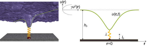
Figure 1: Snapshot from the Langevin simulation of locally pinned membrane fluctuating in a non-specific potential (Left). Sketch of the system (Right). Membrane is residing in a harmonic potential of strength $\gamma$ at $h_{0}$ separation from a flat substrate and pinned by an elastic spring of stiffness $\lambda$ and rest length $l_{0}$ positioned at ${\bf r}=0$.

II Equation of motion

The system consists of one flexible attachment (harmonic spring of an elastic constant $\lambda$ and rest length $l_{0}$) that pins a tensed membrane (bending rigidity $\kappa$, tension $\sigma$). The later fluctuates in a harmonic non-specific potential (strength $\gamma$) positioned at the distance $h_{0}$ above the substrate (Fig. 1). Placing the origin of the coordinate system at the pinning site and into the minimum of the non-specific potential sets the form of the energy functional Schmidt et al. (2012); Janeš et al. (2018) as

$$\mathcal{H}=\int\limits_{A}\mathrm{d}{\bf r} \Bigg{[}\frac{\kappa}{2}\left(\nabla^{2}u({\bf r},t)\right)^{2}+\frac{\sigma}{2}\left(\nabla u({\bf r},t)\right)^{2}+\frac{\gamma}{2}\left(u({\bf r},t)\right)^{2}$$

$$+\frac{1}{2}\lambda\left(u({\bf r},t)-(l_{0}-h_{0})\right)^{2}\delta({\bf r})\Bigg{]}.$$ (1)

Here and throughout the paper, the energy scale $k_{\text{B}}T$ is set to unity, with Boltzmann constant denoted as $k_{\text{B}}$ and absolute temperature $T$.

Dynamics of an overdamped membrane in a hydrodynamic surrounding is captured by the Langevin equation Doi and Edwards (1988); Seifert (1997); Granek (1997); Lin and Brown (2006); Reister-Gottfried et al. (2008); Sigurdsson et al. (2013); Reister et al. (2011); Bihr et al. (2015)

$$\frac{\partial u({\bf r},t)}{\partial t} =\int d{\bf r}^{\prime}\Lambda({\bf r}-{\bf r}^{\prime})\left(-\frac{\delta\mathcal{H}}{\delta u({\bf r}^{\prime},t)}+f({\bf r}^{\prime},t)\right)$$

$$\equiv\Lambda({\bf r})*\left(-\frac{\delta\mathcal{H}}{\delta u({\bf r},t)}+f({\bf r},t)\right),$$ (2)

which states that the velocity of the membrane profile $u({\bf r},t)$ is given by a convolution of the hydrodynamic kernel $\Lambda({\bf r})$, the Oseen tensor, with the forces acting on the membrane. External forces on the system are denoted by $f({\bf r},t)$, while the internal forces acting to minimize the Hamiltonian (eq. (1)) are given by the first variation Janeš et al. (2018)

$$\frac{\delta\mathcal{H}}{\delta u({\bf r},t)}= \left(\kappa\nabla^{4}-\sigma\nabla^{2}+\gamma+\lambda\delta({\bf r})\right)u({\bf r},t)$$

$$- \lambda(l_{0}-h_{0})\delta({\bf r}).$$ (3)

Together with eq. (2), this leads to the equation for the dynamics of an overdamped pinned membrane

$$\mathcal{D}\left[u({\bf r},t)\right]=\Lambda({\bf r})*\left[f({\bf r},t)+\lambda(l_{0}-h_{0})\delta({\bf r})\right],$$ (4)

with the operator $\mathcal{D}$ set as

$$\mathcal{D}=\frac{\partial}{\partial t}+\Lambda({\bf r})*\left(\kappa\nabla^{4}-\sigma\nabla^{2}+\gamma+\lambda\delta({\bf r})\right).$$ (5)

III Time-dependent Green’s function

The solution of eq. (4) provides the evolution of the membrane profile $u({\bf r},t)$. It is obtained by the integration of forces acting on the membrane, the latter accounted for by the dynamic Green’s function $g({\bf r},t|{\bf r}^{\prime},t^{\prime})$

$$u({\bf r},t)= \int_{\mathbb{R}^{2}}\mathrm{d{\bf r}^{\prime}}\int_{\mathbb{R}}\mathrm{dt}^{\prime}\ g({\bf r},t|{\bf r}^{\prime},t^{\prime})\times$$

$$\times\left(f({\bf r}^{\prime},t^{\prime})+\lambda(l_{0}-h_{0})\delta({\bf r}^{\prime})\right).$$ (6)

Here the Green’s function is defined by

$$\mathcal{D}\left[g({\bf r},t|{\bf r}^{\prime},t^{\prime})\right]= \Lambda({\bf r})*\left[\delta({\bf r}-{\bf r}^{\prime})\delta(t-t^{\prime})\right].$$ (7)

Besides imposing causality, this equation is subject to homogeneous spatial boundary conditions forcing the membrane in the minimum of the non-specific potential far from the pinning.

III.1 Free membrane ($\lambda=0$)

Recognizing spatio-temporal translational invariance of the free membrane system, the corresponding Green’s function $g_{f}({\bf r},t|{\bf r}^{\prime},t^{\prime})$ can be written in terms of variables $\tilde{t}=t-t^{\prime}$ and $\tilde{{\bf r}}={\bf r}-{\bf r}^{\prime}$ as

$$g_{f}({\bf r},t|{\bf r}^{\prime},t^{\prime})=g_{f}({\bf r}-{\bf r}^{\prime},t-t^{\prime})\equiv g_{f}(\tilde{{\bf r}},\tilde{t}).$$ (8)

Consequently, for the free membrane eq. (7) becomes

$$\left[\frac{\partial}{\partial\tilde{t}}+\Lambda(\tilde{{\bf r}})*\left(\kappa\nabla_{\tilde{{\bf r}}}^{4}-\sigma\nabla_{\tilde{{\bf r}}}^{2}+\gamma\right)\right]g_{f}(\tilde{{\bf r}},\tilde{t})$$

$$=\Lambda(\tilde{{\bf r}})*\left[\delta(\tilde{{\bf r}})\delta(\tilde{t})\right].$$ (9)

Fourier transforming eq. (9) ($\tilde{{\bf r}}\to{\bf k}$ and $\tilde{t}\to\omega$) upon rearranging yields

$$g_{f}({\bf k},\omega)=\frac{1}{i\omega/\Lambda_{k}+E_{k}},$$ (10)

where $\Lambda_{k}$ is the spatial Fourier transform of $\Lambda(\tilde{{\bf r}}$) and

$$E_{k}=\kappa k^{4}+\sigma k^{2}+\gamma.$$ (11)

Finally, transforming back to the spatio-temporal domain (${\bf k}\to\tilde{{\bf r}}$ and $\omega\to\tilde{t}$) provides the spatio-temporal Green’s function for the free membrane

$$g_{f}(\tilde{{\bf r}},\tilde{t})=\int_{\mathbb{R}^{2}}\frac{d{\bf k}}{(2\pi)^{2}}\int_{\mathbb{R}}\frac{d\omega}{2\pi}\frac{e^{i{\bf k}\tilde{{\bf r}}}e^{i\omega\tilde{t}}}{i\omega/\Lambda_{k}+E_{k}}.$$ (12)

Integrating over the frequencies gives

$$g_{f}(\tilde{{\bf r}},\tilde{t}) =\int\frac{d{\bf k}}{(2\pi)^{2}}\,\Lambda_{k}e^{i{\bf k}\tilde{{\bf r}}}e^{-\Lambda_{k}E_{k}\tilde{t}}\Theta(\tilde{t})$$

$$=\int^{\infty}_{0}\frac{dk}{2\pi}\,\Lambda_{k}kJ_{0}(k|\tilde{{\bf r}}|)e^{-\Lambda_{k}E_{k}\tilde{t}}\Theta(\tilde{t}),$$ (13)

where $\Theta$ is the Heaviside step function appearing as a consequence of causality. Moreover, $g_{f}(\tilde{{\bf r}},\tilde{t})$ depends only on the absolute value of $\tilde{{\bf r}}$, as expected.

For $\omega=0$, the Green’s function $g_{f}(\tilde{{\bf r}},\omega)$ reduces to the static correlation function Janeš et al. (2018). Consequently,

$$g_{f}(\tilde{{\bf r}}=0,\omega=0)\equiv\frac{1}{\lambda_{m}}=\frac{\text{arctan}\left(\sqrt{\left(\frac{\lambda_{m}^{0}}{4\sigma}\right)^{2}-1}\right)}{2\pi\sigma\sqrt{\left(\frac{\lambda_{m}^{0}}{4\sigma}\right)^{2}-1}}$$ (14)

represents the fluctuation amplitude, which in the tensionless case reduces to

$$g_{f}(\tilde{{\bf r}}=0,\omega=0;\sigma=0)\equiv\frac{1}{\lambda^{0}_{m}}=\frac{1}{8\sqrt{\kappa\gamma}}.$$ (15)

III.2 Pinned membrane

Permanent pinning breaks the spatial, but keeps the temporal translational invariance. Therefore, the Green’s function of the pinned membrane must be described by two spatial variables ${\bf r}$ and ${\bf r}^{\prime}$ and one temporal variable $\tilde{t}=t-t^{\prime}$

$$g({\bf r},t|{\bf r}^{\prime},t^{\prime})=g({\bf r},t-t^{\prime}|{\bf r}^{\prime})\equiv g({\bf r},\tilde{t}|{\bf r}^{\prime}).$$ (16)

In this notation, eq. (7) for the pinned membrane Green’s function becomes

$$\left[\frac{\partial}{\partial\tilde{t}}+\Lambda({\bf r})*\left(\kappa\nabla^{4}-\sigma\nabla^{2}+\gamma+\lambda\delta({\bf r})\right)\right]g({\bf r},\tilde{t}|{\bf r}^{\prime})$$

$$=\Lambda({\bf r})*\left[\delta({\bf r}-{\bf r}^{\prime})\delta(\tilde{t})\right].$$ (17)

Fourier transforming (${\bf r}\to{\bf k}$ and $\tilde{t}\to\omega$) and rearranging eq. (17) gives

$$g({\bf k},\omega|{\bf r}^{\prime})=\frac{e^{-i{\bf k}{\bf r}^{\prime}}}{i\omega/\Lambda_{k}+E_{k}}-\lambda g({\bf r}=0,\omega|{\bf r}^{\prime})\frac{1}{i\omega/\Lambda_{k}+E_{k}}.$$ (18)

Transforming back to the spatial domain (${\bf k}\to{\bf r}$) gives

$$g({\bf r},\omega|{\bf r}^{\prime})= g_{f}({\bf r}-{\bf r}^{\prime},\omega)-\lambda g({\bf r}=0,\omega|{\bf r}^{\prime})g_{f}({\bf r},\omega).$$ (19)

For ${\bf r}=0$ in eq. (19) we find

$$g({\bf r},\omega|{\bf r}^{\prime})=\frac{g_{f}({\bf r}^{\prime},\omega)}{1+\lambda g_{f}({\bf r}=0,\omega)},$$ (20)

which upon inserting into (19) yields the Green’s function for the pinned membrane in the spatio-frequency domain

$$g({\bf r},\omega|{\bf r}^{\prime})=g_{f}({\bf r}-{\bf r}^{\prime},\omega)-\lambda\frac{g_{f}({\bf r},\omega)g_{f}({\bf r}^{\prime},\omega)}{1+\lambda g_{f}({\bf r}=0,\omega)}.$$ (21)

Fourier transforming eq. (21) (${\bf r}\to{\bf k}$ and ${\bf r}^{\prime}\to{\bf k}^{\prime}$) results in

$$g({\bf k},\omega|{\bf k}^{\prime})=(2\pi)^{2}\delta({\bf k}+{\bf k}^{\prime})g_{f}({\bf k},\omega)-\lambda\frac{g_{f}({\bf k},\omega)g_{f}({\bf k}^{\prime},\omega)}{1+\lambda g_{f}({\bf r}=0,\omega)},$$ (22)

which is the representation of the Green’s function in the Fourier space.

IV Dynamics of thermal fluctuations

IV.1 Oseen tensor

In thermal equilibrium $f({\bf r},t)$ is associated with the stochastic thermal noise characterized by a vanishing mean

$$\langle f({\bf r},t)\rangle=0$$ (23)

and spatio-temporal correlations obeying the fluctuation-dissipation theorem

$$\langle f({\bf r},t)f({\bf r}^{\prime},t^{\prime})\rangle=2\Lambda^{-1}({\bf r}-{\bf r}^{\prime})\delta(t-t^{\prime}).$$ (24)

Here $\Lambda^{-1}({\bf r})$ is defined by

$$\Lambda({\bf r})*\Lambda^{-1}({\bf r})=\delta({\bf r}).$$ (25)

To model damping of the membrane due to hydrodynamic interactions with the surrounding fluid close to a wall Doi and Edwards (1988); Lin and Brown (2006), we will use the Fourier transform of the Oseen tensor $\Lambda_{k}$

$$\Lambda_{k}=(4\eta k)^{-1},$$ (26)

where $\eta$ is the viscosity of the surrounding fluid. Eq. (26) is appropriate when the wall is permeable to the fluid. In the presence of an impermeable wall, damping coefficients are modified Seifert (1994); Gov et al. (2003), which in the case of protein mediated adhesion, typically has an effect only on the amplitude of the first few membrane modes Reister-Gottfried et al. (2008). Furthermore, if the membrane is surrounded by two different fluids with viscosities $\eta_{1}$ and $\eta_{2}$, the viscosity $\eta$ in the damping coefficients is replaced by the arithmetic mean $\eta=(\eta_{1}+\eta_{2})/2$ Monzel et al. (2016).

IV.2 Simulation methods

Eq. (4) for the membrane dynamics, subject to thermal noise defined with eqs. (23)-(26), is the foundation of our Langevin dynamics simulations of the membrane, described previously in full detail Bihr et al. (2015). In the current case, one pinning site is placed in a middle of the simulation box (periodic boundary conditions) of a size of $640\times 640$ nm for a tensionless membrane, and a size of $5120\times 5120$ nm at finite tensions. The simulations are performed with a temporal and lateral resolution of $10^{-9}$ s and $10$ nm, respectively. The membrane height profile is recorded as a function of time and analyzed to extract the membrane shape and correlation functions.

IV.3 Power Spectral Density

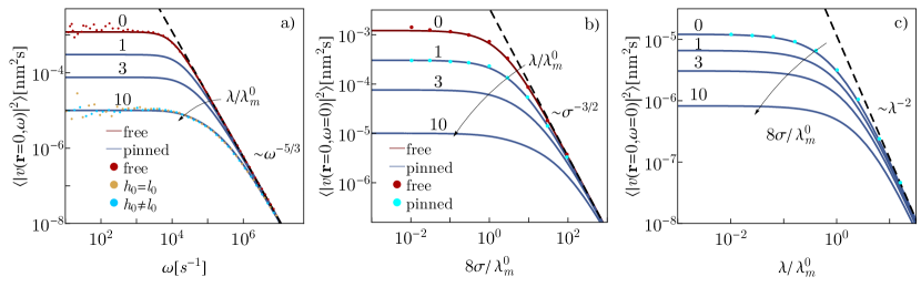
Figure 2: Dynamical properties of a membrane at the pinning site. Comparison of modelling (lines) and simulations (symbols) shows excellent agreement across the entire parameter range. a) Power spectral density of a free membrane (eq. (33)) (red) and a pinned tensionless membrane eq. (35) (blue dashed curves for $\lambda/\lambda_{m}^{0}=1,3,10$, increasing in the direction of the arrows). The high-frequency regime of the PSD is unaffected by the pinning and the free-membrane behaviour ($\omega^{-5/3}$) is recovered. b) Low frequency limit of the PSD (eq. (36)) as a function of the membrane tension $\sigma$ for different pinning strengths ($\lambda/\lambda_{m}^{0}=1,3,10$). For large tensions, a $\sigma^{-3/2}$ dependence is recovered irrespective of $\lambda$. c) Low frequency limit as a function of the pinning strength for different membrane tensions ($8\sigma/\lambda_{m}^{0}=1,3,10$). For large bond stiffness, a $\lambda^{-2}$ dependence is displayed. All curves are plotted for $\kappa=20k_{\text{B}}T$, $\gamma=3\times 10^{-7}k_{\text{B}}T/$nm⁴ and $\eta=1$ mPas.

We complement the simulations of thermally fluctuating membrane with the analytic calculations based on the Green’s function approach (eq. (6)). We start with rewriting eq. (6) as

$$u({\bf r},t)=\langle u({\bf r})\rangle+v({\bf r},t),$$ (27)

where

$$v({\bf r},t)= \int_{\mathbb{R}^{2}}\mathrm{d{\bf r}^{\prime}}\int_{\mathbb{R}}\mathrm{dt}^{\prime}\ g({\bf r},t-t^{\prime}|{\bf r}^{\prime})f({\bf r}^{\prime},t^{\prime})$$ (28)

are the fluctuations around the ensemble averaged static profile Janeš et al. (2018)

$$\langle u({\bf r})\rangle= \int_{\mathbb{R}^{2}}\mathrm{d{\bf r}^{\prime}}\int_{\mathbb{R}}\mathrm{dt}^{\prime}\ g({\bf r},t-t^{\prime}|{\bf r}^{\prime})\lambda(l_{0}-h_{0})\delta({\bf r}^{\prime}).$$ (29)

Transforming ($t\to\omega$) eq. (28) gives

$$v({\bf r},\omega) =\int_{\mathbb{R}^{2}}\mathrm{d{\bf r}^{\prime}}\ g({\bf r},\omega|{\bf r}^{\prime})f({\bf r}^{\prime},\omega)$$ (30)

from which the PSD $\langle|v({\bf r},\omega)|^{2}\rangle$ can be calculated as (see Supplementary Information)

$$\langle|v({\bf r},\omega)|^{2}\rangle= \frac{1}{(2\pi)^{2}}\int_{\mathbb{R}^{2}}\mathrm{d{\bf k}}\frac{2\Lambda_{k}^{-1}}{(\omega/\Lambda_{k})^{2}+E^{2}_{k}}\times$$

$$\times\left|1-\frac{\lambda g_{f}({\bf r},\omega)}{1+\lambda g_{f}({\bf r}=0,\omega)}e^{-i{\bf k}{\bf r}}\right|^{2}.$$ (31)

With the hydrodynamic coefficients specified as in eq. (26), eq. (31) becomes

$$\langle|v({\bf r},\omega)|^{2}\rangle= \frac{4\eta}{\pi}\int\limits_{0}^{\infty}\mathrm{d}k\frac{k^{2}}{(4\eta k\omega)^{2}+(\kappa k^{4}+\sigma k^{2}+\gamma)^{2}}\times$$

$$\times\left|1-\frac{\lambda g_{f}({\bf r},\omega)}{1+\lambda g_{f}({\bf r}=0,\omega)}e^{-i{\bf k}{\bf r}}\right|^{2}.$$ (32)

In the absence of the pinning ($\lambda=0$), eq. (32) becomes homogeneous in space and reduces to the well-known result

$$\left\langle|v_{f}(\omega)|^{2}\right\rangle =\frac{4\eta}{\pi}\int\limits_{0}^{\infty}\mathrm{d}k\frac{k^{2}}{(4\eta k\omega)^{2}+(\kappa k^{4}+\sigma k^{2}+\gamma)^{2}},$$ (33)

which for small and large $\omega$ has the limiting behaviour Brochard and Lennon (1975); E. Helfer (2000); Betz et al. (2009); Betz and Sykes (2012)

$$\langle|v_{f}(\omega)|^{2}\rangle=\begin{cases}\frac{\eta}{\sqrt{\gamma(\lambda_{m}^{0}/4+\sigma)^{3}}},&\omega\ll\omega_{0}\\ \frac{1}{6\sqrt[3]{2\eta^{2}\kappa}}\omega^{-5/3},&\omega\gg\omega_{0}.\end{cases}$$ (34)

Here, $\omega_{0}\equiv\sqrt[4]{\kappa\gamma^{3}}/\eta$ is a cross-over frequency, defined as the intersection of the lines fitting the low- and high-frequency limits of the spectrum. The low-frequency limit decays with $\sigma^{-3/2}$ for tensions $\sigma\gg\lambda_{m}^{0}$ (Fig. 2b).

It is clear from Eq. (32) that the PSD at the pinning site ${\bf r}=0$ can be recast into

$$\langle|v({\bf r}=0,\omega)|^{2}\rangle =\left|\frac{1}{1+\lambda g_{f}({\bf r}=0,\omega)}\right\rvert^{2}\langle|v_{f}(\omega)|^{2}\rangle.$$ (35)

In agreement with simulations based on eqs. (4), (23) and (24) Bihr et al. (2015), eq. (35) shows that only the pinning stiffness, and not its length, has an effect on the PSD and that the pinning affects only the low-frequency regime (Fig. 2a). The low-frequency behaviour can be obtained upon combining eq. (35) for $\omega=0$ with eq. (34) to yield

$$\langle|v({\bf r}=0,\omega=0)|^{2}\rangle=\left(\frac{1}{1+\lambda/\lambda_{m}}\right)^{2}\frac{\eta}{\sqrt{\gamma(\lambda_{m}^{0}/4+\sigma)^{3}}}$$

$$= \begin{cases}\left(\frac{1}{1+\lambda/\lambda^{0}_{m}}\right)^{2}\frac{\eta}{\sqrt{\gamma(\lambda^{0}_{m}/4)^{3}}},&\quad 4\sigma/\lambda_{m}^{0}\ll 1\\ \left(\frac{1}{1+\lambda\ln(\sigma)/(2\pi\sigma)}\right)^{2}\frac{\eta}{\sqrt{\gamma\sigma^{3}}},&\quad 4\sigma/\lambda_{m}^{0}\gg 1.\end{cases}$$ (36)

Eq. (36) shows that the low-frequency spectrum is independent of membrane tension for $4\sigma/\lambda_{m}^{0}\ll 1$ and it decays with $\sigma^{-3/2}$ for membrane tensions large enough to diminish the effect of the pinning ($\lambda\ln(\sigma)/(2\pi\sigma)\ll 1$) (Fig. 2b). For stiff pinnings ($\lambda/\lambda_{m}\gg 1$) the low-frequency limit falls off as $\lambda^{-2}$ (Fig. 2c). On the other hand, for $\lambda/\lambda_{m}\ll 1$, pinning effects vanish even in the low-frequency limit. Interestingly, the cross-over frequency $\tilde{\omega}_{0}$ for the pinned membrane

$$\tilde{\omega}_{0} =\left[6\sqrt[3]{2\eta^{2}\kappa}\ \langle|v({\bf r}=0,\omega=0)|^{2}\rangle\right]^{-3/5},$$ (37)

defined analogously to the one for the free membrane, becomes sensitive to the elastic properties of the pinning as $\tilde{\omega}_{0}\sim\lambda^{6/5}$ and as such increases with the pinning stiffness.

V Effect of the finite experimental resolution on the fluctuation spectrum

In order to compare with experiments, it is necessary to account for the finite temporal and spatial resolutions of the set-up Pécréaux et al. (2004); Monzel et al. (2016). Averaging the true membrane profile $u({\bf r},t)$ over a spatial domain $A$ and a time interval ${\tau}$, gives rise the so-called apparent membrane profile $u^{A}_{\tau}({\bf r},t)$

$$u^{A}_{\tau}({\bf r},t)=\int\limits_{0}^{\tau}\frac{\mathrm{d}t^{\prime}}{{\tau}}\int\limits_{A}\frac{\mathrm{d}{\bf r}^{\prime}}{A}u({\bf r}+{\bf r}^{\prime},t+t^{\prime}),$$ (38)

from which it is straightforward to derive the apparent PSD (Supplementary Information, section I. A)

$$\langle| v^{A}_{\tau}({\bf r},\omega)|^{2}\rangle=\left(\frac{\sin(\omega{\tau}/2)}{\omega{\tau}/2}\right)^{2}\frac{2}{(2\pi)^{2}}\times$$

$$\times\int_{\mathbb{R}^{2}}\mathrm{d{\bf k}}\ \frac{\Lambda_{k}^{-1}}{(\omega/\Lambda_{k})^{2}+E^{2}_{k}}\left|\int\limits_{A}\frac{\mathrm{d}{\bf r}^{\prime}}{A}e^{i{\bf k}({\bf r}+{\bf r}^{\prime})}\right.\times$$

$$\times\left.\left(1-\frac{\lambda g_{f}({\bf r}+{\bf r}^{\prime},\omega)}{1+\lambda g_{f}(0,\omega)}e^{-i{\bf k}({\bf r}+{\bf r}^{\prime})}\right)\right|^{2}.$$ (39)

The PSD measured around the pinning placed centrally in a circle of radius $R$ is (Supplementary Information, section I. A.1.)

$$\langle|v^{R^{2}\pi}_{\tau}({\bf r}=0,\omega)|^{2}\rangle=\left(\frac{\sin(\omega{\tau}/2)}{\omega{\tau}/2}\right)^{2}\frac{1}{\pi}\times$$

$$\times \int\limits^{\infty}_{0}\mathrm{dk}\ \frac{k\Lambda_{k}^{-1}}{(\omega/\Lambda_{k})^{2}+E^{2}_{k}}\rule{0.0pt}{22.76228pt}\frac{4}{R^{2}}$$

$$\times \rule{0.0pt}{22.76228pt}\left|\frac{J_{1}(kR)}{k}-\frac{\lambda}{1+\lambda g_{f}(0,\omega)}\frac{1}{2\pi}\int\limits^{\infty}_{0}\mathrm{dk^{\prime}}\frac{J_{1}(k^{\prime}R)}{i\omega/\Lambda_{k^{\prime}}+E_{k^{\prime}}}\right|^{2}.$$ (40)

Eq. (40) reduces to eq. (35) in the limit ${\tau},R\to 0$.

The high frequency regime of the averaged PSD recovers the averaging behaviour of the free membrane - spatial averaging changes the decay from $\omega^{-5/3}$ to $\omega^{-2}$ as previously reported Betz and Sykes (2012), while finite temporal resolution induces an additional attenuation of $\omega^{-2}$. Hence, the PSD which is subject to both temporal and spatial averaging decays as $\omega^{-4}$.

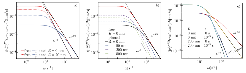
Figure 3: Effect of the finite resolution (averaging over a circle of radius $R$ and a time interval $\tau$) on the PSD at the pinning (eq. (40)). a) Averaging decreases the difference between the free and pinned PSD’s, therefore reducing the effect of the pinning on the PSD. Pinning has no effect on the high-frequency part of the spectrum, for both the averaged and the unaveraged spectrum. b) The low-frequency part of the PSD is a non-monotone function of the spatial averaging area. On the other hand, increasing the averaging area always attenuates the high-frequency components, which in this case fall as $\sim\omega^{-2}$ instead of $\sim\omega^{-5/3}$. c) Time averaging introduces oscillatory behaviour of the PSD for which only the envelope of the PSD is shown. The combined effect of the spatial and temporal averaging gives a $\sim\omega^{-4}$ behaviour of the high-frequency regime . Parameters $\kappa=20k_{\text{B}}T$, $\sigma=10^{-20}k_{\text{B}}T/\text{nm}^{2}$ and $\gamma=3\times 10^{-7}k_{\text{B}}T/$nm⁴, $\lambda/\lambda^{0}_{m}$=10 and $\eta=1\,\mathrm{mPas}$.

In the low frequency regime, temporal averaging plays no role for $\omega<1/{\tau}$, while the finite spatial resolution has a more complex effect. Due to the interplay with the effects of the pinning, the low frequency amplitude is not a monotone function of the averaging area (Fig. 3). Increasing the averaging area up to some critical size (which is approximately the area affected by the pinning) amplifies the low-frequency components, but further increase of the averaging area starts to attenuate them. This can be understood as a competition of two effects; averaging has the effect of attenuating the low frequency components, as can be seen for the free membrane, but at the same time, averaging reduces the effect of the pinning on the PSD, which amplifies the low-frequency components. Obviously, the later effect is stronger up to the critical averaging area size, after which the first effect dominates. Specifically, for $\omega=0$ we obtain (Supplementary Information, section I.A.1)

$$\langle|v^{R^{2}\pi}_{\tau}({\bf r}=0,0)|^{2}\rangle=$$

$$=\frac{4\eta}{\pi}\int\limits^{\infty}_{0}\mathrm{dk}\ \frac{k^{2}}{E^{2}_{k}}\left|\frac{J_{1}(kR)}{kR/2}-\frac{\lambda}{1+\lambda/\lambda_{m}}s(R)\right|^{2},$$ (41)

where for brevity purposes we introduce a reduced coefficient $s(R)$

$$s(R) =\frac{1}{R^{2}\pi\sqrt{\sigma-4\kappa\gamma}}\times$$

$$\times \left(\frac{1-a_{-}RK_{1}(a_{-}R)}{a^{2}_{-}}-\frac{1-a_{+}RK_{1}(a_{+}R)}{a^{2}_{+}}\right),$$ (42)

with $a_{\pm}$

$$a_{\pm} =\left[\frac{\sigma}{2\kappa}\left(1\pm\sqrt{1-\left(\frac{\lambda_{m}^{0}}{4\sigma}\right)^{2}}\right)\right]^{1/2}.$$ (43)

In order to calculate the pinning stiffness $\lambda$ from the PSD, eq. (41) can be inverted, which upon introduction of coefficients $L$, $a$, $b$ and $c$, yields

$$\lambda=\left(\dfrac{1}{L}-\frac{1}{\lambda_{m}}\right)^{-1},$$ (44)

with

$$L=\frac{b}{2a}-\sqrt{\left(\frac{b}{2a}\right)^{2}-\frac{c}{a}}$$ (45)

and

$$a= \frac{\pi s^{2}(R)}{4\sqrt{\gamma(\lambda_{m}^{0}/4+\sigma)^{3}}},$$

$$b= \frac{4s(R)}{R}\left(\int\limits^{\infty}_{0}\mathrm{dk}\frac{kJ_{1}(kR)}{E^{2}_{k}}\right),$$

$$c= \left(\frac{2}{R}\right)^{2}\int\limits^{\infty}_{0}\mathrm{dk}\frac{J_{1}^{2}(kR)}{E^{2}_{k}}-\frac{\pi}{4\eta}\langle|v^{R^{2}\pi}_{\tau}({\bf r}=0,0)|^{2}\rangle.$$ (46)

The averaged spectrum is contained in the coefficient $c$. When implemented numerically, eqs. (44-46) represent a fast and exact method for obtaining information about the pinning stiffness from the experimentally measured PSD. Here we note that the deconvolution of the noise associated with the experimental setting should be performed prior to the extraction of the pinning stiffness.

VI Discussion and Conclusion

Our calculation of the Green’s function (eq. (21)) fully resolves the dynamics of an overdamped, permanently pinned membrane in a hydrodynamic surrounding (eq. (2)). The solution is general in a sense that it works for any forces acting on the membrane and enables one to study the membrane dynamics in the presence of both non-thermal and thermal perturbations. The later case is resolved in this paper by the calculation of the thermal equilibrium power spectral density (eq. (31)). For the specific case of hydrodynamic damping close to a permeable wall, our analytical calculation (eq. (32)) is verified with Langevin simulations in a broad range of parameters, such as the pinning stiffness, membrane tension, and strength of the non-specific potential, which were allowed to independently vary for several orders of magnitude (Fig. 2). It is shown that the pinning decreases the low-frequency amplitudes of the spectrum and pushes the cross-over frequency (eq. (37)) to higher values, while the high-frequency amplitudes remain unaffected (Fig. 2).

Interestingly, the pinned-membrane PSD at the pinning site is given by a product of a free-membrane PSD and a $\lambda$-dependent prefactor (eq. (35)). Assuming knowledge of the pinning stiffness $\lambda$, this enables inference of the pinned-membrane PSD at the pinning site directly from the free-membrane PSD. This approach has a clear advantage over a direct measurement of the pinned-PSD, as it replaces the pinned-membrane measurement, with a well-established free membrane measurement. On the other hand, if $\lambda$ is not known, it can be easily determined by comparing the pinned- and free-membranes PSDs. The low-frequency limit of the PSD at the pinning site (eq. (36)) is particularly useful for getting a better understanding of the interplay of the system parameters and shows a $\lambda^{-2}$ decay.

These relationships, however, may not be observed experimentally due to the finite resolution of the measurements. Specifically, while the effects of the temporal averaging are simple, significant spatial averaging introduces nontrivial modulations of the spectrum and breaks the relation between the free- and the pinned-membrane PSD given by eq. (35). In this regime the pinning stiffness can be inferred from the measured PSD with the use of the spatially averaged spectrum (eqs. (44-46)).

A deep understanding of the mechanics of the pinned membrane is crucial for elucidating the role of more complex pinnings, which under typical biological conditions stochastically bind and unbind from the membrane. The stochasticity of this attachment will have additional effects on fluctuations of the membrane which could not be resolved prior to this investigation, and will be subject to a future study. The results presented in this paper will thus help establishing the connection between functioning of the protein assembly and the properties of the elastic fluctuating membrane, which is important for understanding of the formation of adhesions. Namely, there is a growing body of evidence that the membrane affects the affinity Huppa et al. (2010) and the kinetic rates for protein binding Bihr et al. (2015); Fenz et al. (2017), which in turn affect the fluctuations and the early stage signalling in developing junctions between cells Perez et al. (2008).

The model presented here can be used to measure the elasticity of the bond from membrane fluctuations. Hitherto, it was not possible to interpret these measurements accurately, a task that is enabled now by our current work. Such measurements could then be compared to AFM measurements, which are commonly used to study elastic properties of the linkers.

Acknowledgments: A.-S.S and J.A.J. thank ERCStg MembranesAct for support as well as the Croatian Science Foundation research project CompSoLs MolFlex 8238. A.-S.S and D.S. were supported by the Research Training Group 1962 at the Friedrich-Alexander-Universität Erlangen-Nürnberg.

References

- Helfrich (1973) W. Helfrich, “Elastic properties of lipid bilayers: Theory and possible experiments,” Z. Naturforsch., C: J. Biosci. 28, 693–703 (1973).
- Helfrich (1978) W. Helfrich, “Steric interaction of fluid membranes in multilayer systems,” Z. Naturforsch., A: Phys. Sci. 33, 305 (1978).
- Lipowsky and Sackmann (1995) R. Lipowsky and E. Sackmann, eds., Structure and dynamics of membranes (Elsevier, 1995).
- Smith et al. (2006) A.-S. Smith, B.G. Lorz, S. Goennenwein, and E. Sackmann, “Force-controlled equilibria of specific vesicle-substrate adhesion,” Biophys. J. 90, L52–L54 (2006).
- Monzel et al. (2012) C. Monzel, S. F. Fenz, M. Giesen, R. Merkel, and K. Sengupta, “Mapping fluctuations in biomembranes adhered to micropatterns,” Soft Matter 8, 6128–6138 (2012).
- Marx et al. (2002) S. Marx, J. Schilling, E. Sackmann, and R. Bruinsma, “Helfrich repulsion and dynamical phase separation of multicomponent lipid bilayers,” Phys. Rev. Lett. 88, 138102 (2002).
- Monzel and Sengupta (2016) C. Monzel and K. Sengupta, “Measuring shape fluctuations in biological membranes,” J. Phys. D: Appl. Phys. 49, 243002 (2016).
- Fenz and Sengupta (2012) S. F. Fenz and K. Sengupta, “Giant vesicles as cell models,” Integr. Biol. 4, 982–995 (2012).
- Betz and Sykes (2012) T. Betz and C. Sykes, “Time resolved membrane fluctuation spectroscopy,” Soft Matter 8, 5317–5326 (2012).
- Schmidt et al. (2014) D. Schmidt, C. Monzel, T. Bihr, R. Merkel, U. Seifert, K. Sengupta, and A.-S. Smith, “Signature of a nonharmonic potential as revealed from a consistent shape and fluctuation analysis of an adherent membrane,” Phys. Rev. X 4, 021023 (2014).
- Brochard and Lennon (1975) F. Brochard and J. F. Lennon, “Frequency spectrum of the flicker phenomenon in erythrocytes,” J. Phys. France 36, 11 (1975).
- Kramer (1971) L. Kramer, “Theory of light scattering from fluctuations of membranes and monolayers,” J. Chem. Phys. 55, 2097–2105 (1971).
- Seifert and Langer (1993) U. Seifert and S.A. Langer, “Viscous modes of fluid bilayer membranes,” Europhys. Lett. 23, 71 (1993).
- Atzberger (2011) P. J. Atzberger, “Stochastic eulerian lagrangian methods for fluid–structure interactions with thermal fluctuations,” Journal of Computational Physics 230, 2821 – 2837 (2011).
- Monzel et al. (2016) C. Monzel, D. Schmidt, U. Seifert, A.-S. Smith, R. Merkel, and K. Sengupta, “Nanometric thermal fluctuations of weakly confined biomembranes measured with microsecond time-resolution,” Soft Matter 12, 4755–4768 (2016).
- Helfrich and Servuss (1984) W. Helfrich and R.-M. Servuss, “Undulations, steric interaction and cohesion of fluid membranes,” Nuovo Cimento D 3, 137–151 (1984).
- Evans and Parsegian (1986) E. A. Evans and V. A. Parsegian, “Thermal-mechanical fluctuations enhance repulsion between bimolecular layers,” Proc. Natl. Acad. Sci. U. S. A. 83, 7132 (1986).
- Israelachvili and Wennerstroem (1992) J. N. Israelachvili and H. Wennerstroem, “Entropic forces between amphiphilic surfaces in liquids,” J. Phys. Chem. 96, 520–531 (1992).
- Rädler et al. (1995) J. O. Rädler, T. J. Feder, H. H. Strey, and E. Sackmann, “Fluctuation analysis of tension-controlled undulation forces between giant vesicles and solid substrates,” Phys. Rev. E 51, 4526–4536 (1995).
- Seifert (1997) U. Seifert, “Configurations of fluid membranes and vesicles,” Adv. Phys. 46, 13–137 (1997).
- Lorz et al. (2007) B. G. Lorz, A.-S. Smith, C. Gege, and E. Sackmann, “Adhesion of giant vesicles mediated by weak binding of sialyl-lewisx to e-selectin in the presence of repelling poly(ethylene glycol) molecules,” Langmuir 23, 12293–12300 (2007).
- Safran et al. (2005) S. A. Safran, N. Gov, A. Nicolas, U. S. Schwarz, and T. Tlusty, “Physics of cell elasticity, shape and adhesion,” Physica A 352, 171 (2005).
- Betz et al. (2009) T. Betz, M. Lenz, J.-F. Joanny, and C. Sykes, “Atp-dependent mechanics of red blood cells,” Proc. Natl. Acad. Sci. U. S. A. 106, 15320–15325 (2009).
- Monzel et al. (2015) C. Monzel, D. Schmidt, C. Kleusch, D. Kirchenbüchler, U. Seifert, A.-S. Smith, K. Sengupta, and R. Merkel, “Measuring fast stochastic displacements of bio-membranes with dynamic optical displacement spectroscopy,” Nat. Commun. 6, 8162 (2015).
- Prost et al. (1998) J. Prost, J.-B. Manneville, and R. Bruinsma, “Fluctuation-magnification of non-equilibrium membranes near a wall,” Eur. Phys. J. B 1, 465–480 (1998).
- Ramaswamy et al. (2000) S. Ramaswamy, J. Toner, and J.s Prost, “Nonequilibrium fluctuations, traveling waves, and instabilities in active membranes,” Phys. Rev. Lett. 84, 3494 (2000).
- Manneville et al. (2001) J.-B. Manneville, P. Bassereau, S. Ramaswamy, and J. Prost, “Active membrane fluctuations studied by micropipet aspiration,” Phys. Rev. E 64, 021908 (2001).
- Girard et al. (2005) P. Girard, J. Prost, and P. Bassereau, “Passive or active fluctuations in membranes containing proteins,” Phys. Rev. Lett. 94, 088102 (2005).
- Gov and Safran (2005) N. S. Gov and S. A. Safran, “Red blood cell membrane fluctuations and shape controlled by atp-induced cytoskeletal defects,” Biophys. J. 88, 1859–1874 (2005).
- Lin et al. (2006) L. C.-L. Lin, N. Gov, and F. L. H. Brown, “Nonequilibrium membrane fluctuations driven by active proteins,” J. Chem. Phys. 124, 074903 (2006).
- Loubet et al. (2012) B. Loubet, U. Seifert, and M. A. Lomholt, “Effective tension and fluctuations in active membranes,” Phys. Rev. E 85, 031913 (2012).
- Hanlumyuang et al. (2014) Y. Hanlumyuang, L. P. Liu, and P. Sharma, “Revisiting the entropic force between fluctuating biological membranes,” J. Mech. Phys. Solids 63, 179–186 (2014).
- Alert et al. (2015) R. Alert, J. Casademunt, J. Brugués, and P. Sens, “Model for probing membrane-cortex adhesion by micropipette aspiration and fluctuation spectroscopy,” Biophys. J. 108, 1878–1886 (2015).
- Mizuno et al. (2007) D. Mizuno, C. Tardin, C. F. Schmidt, and F. C. MacKintosh, “Nonequilibrium mechanics of active cytoskeletal networks,” Science 315, 370–373 (2007).
- Ben-Isaac et al. (2011) E. Ben-Isaac, Y. Park, G. Popescu, F. L. H. Brown, N. S. Gov, and Y. Shokef, “Effective temperature of red-blood-cell membrane fluctuations,” Phys. Rev. Lett. 106, 238103 (2011).
- Turlier et al. (2016) H. Turlier, D. A. Fedosov, B. Audoly, T. Auth, N. S. Gov, C. Sykes, J.-F. Joanny, G. Gompper, and T. Betz, “Equilibrium physics breakdown reveals the active nature of red blood cell flickering,” Nat. Phys. (2016), 10.1038/nphys3621.
- Gov and Safran (2004) N. Gov and S. Safran, “Pinning of fluid membranes by periodic harmonic potentials,” Phys. Rev. E 69, 011101 (2004).
- Lin and Brown (2005) L. C.-L. Lin and F. L. H. Brown, “Dynamic simulations of membranes with cytoskeletal interactions,” Phys. Rev. E 72, 011910 (2005).
- Reister et al. (2011) E. Reister, T. Bihr, U. Seifert, and A.-S. Smith, “Two intertwined facets of adherent membranes: membrane roughness and correlations between ligand–receptors bonds,” New J. Phys. 13, 025003:1–15 (2011).
- Hu et al. (2013) J. Hu, R. Lipowsky, and T. R. Weikl, “Binding constants of membrane-anchored receptors and ligands depend strongly on the nanoscale roughness of membranes,” Proc. Natl. Acad. Sci. U. S. A. 110, 15283–15288 (2013).
- Bihr et al. (2015) T. Bihr, U. Seifert, and A.-S. Smith, “Multiscale approaches to protein-mediated interactions between membranes—relating microscopic and macroscopic dynamics in radially growing adhesions,” New J. Phys. 17, 083016 (2015).
- Bruinsma et al. (1994) R. Bruinsma, M. Goulian, and P. Pincus, “Self-assambly of membrane junctions,” Biophys. J. 67, 746–750 (1994).
- Janeš et al. (2018) J. A. Janeš, H. Stumpf, Schmidt D., Seifert U., and Smith A.-S., “Statistical mechanics of an elastically pinned membrane: Static profile and correlations,” ArXiv e-prints (2018), arXiv:1806.05109 [physics.bio-ph] .
- Lin and Brown (2004) L. C.-L. Lin and F. L. H. Brown, “Dynamics of pinned membranes with application to protein diffusion on the surface of red blood cells,” Biophys. J. 86, 764–780 (2004).
- Schmidt et al. (2012) D. Schmidt, T. Bihr, U. Seifert, and A.-S. Smith, “Coexistence of dilute and densely packed domains of ligand-receptor bonds in membrane adhesion,” Europhys. Lett. 99, 38003 (2012).
- Doi and Edwards (1988) M. Doi and S.F. Edwards, The Theory of Polymer Dynamics, Vol. 73 (Oxford University Press, 1988).
- Granek (1997) R. Granek, “From semi-flexible polymers to membranes: Anomalous diffusion and reptation,” Journal de Physique II 12, 1761 (1997).
- Lin and Brown (2006) L. C.-L. Lin and F. L. H. Brown, “Simulating membrane dynamics in nonhomogeneous hydrodynamic environments,” J. Chem. Theory Comput. 2, 472–483 (2006).
- Reister-Gottfried et al. (2008) E. Reister-Gottfried, K. Sengupta, B. Lorz, E. Sackmann, U. Seifert, and A.-S. Smith, “Dynamics of specific vesicle-substrate adhesion: From local events to global dynamics,” Phys. Rev. Lett. 101, 208103:1–4 (2008).
- Sigurdsson et al. (2013) J. K. Sigurdsson, F. L. H. Brown, and P. J. Atzberger, “Hybrid continuum-particle method for fluctuating lipid bilayer membranes with diffusing protein inclusions,” Journal of Computational Physics 252, 65 – 85 (2013).
- Seifert (1994) U. Seifert, “Dynamics of a bound membrane,” Phys. Rev. E 49, 3124–3127 (1994).
- Gov et al. (2003) N. Gov, A. G. Zilman, and S. Safran, “Cytoskeleton confinement and tension of red blood cell membranes,” Phys. Rev. Lett. 90, 228101 (2003).
- E. Helfer (2000) L. Bourdieu J. Robert F. C. MacKintosh D. Chatenay E. Helfer, S. Harlepp, “Microrheology of biopolymer-membrane complexes.” Phys. Rev. Lett. 85, 457 (2000).
- Pécréaux et al. (2004) J. Pécréaux, H.-G. Döbereiner, J. Prost, J.-F. Joanny, and P. Bassereau, “Refined contour analysis of giant unilamellar vesicles,” Eur. Phys. J. E 13, 277–290 (2004).
- Huppa et al. (2010) J. B. Huppa, M. Axmann, M. A. Mörtelmaier, B. F. Lillemeier, E. W. Newell, M. Brameshuber, L. O. Klein, G. J. Schütz, and M. M. Davis, “TCR–peptide–MHC interactions in situ show accelerated kinetics and increased affinity,” Nature 463, 963 (2010).
- Fenz et al. (2017) S. Fenz, T. Bihr, D. Schmidt, R. Merkel, U. Seifert, K. Sengupta, and A.-S. Smith, “Membrane fluctuations mediate lateral interactions between cadherin bonds,” Nature Physics 13, 906–913 (2017).
- Perez et al. (2008) Tomas D. Perez, Masako Tamada, Michael P. Sheetz, and W. James Nelson, “Immediate-early signaling induced by e-cadherin engagement and adhesion,” Journal of Biological Chemistry 283, 5014–5022 (2008).