Einstein-Podolski-Rosen steering is a form of quantum correlation exhibiting an intrinsic asymmetry between two entangled systems. In this paper, we propose a scheme for examining dynamical Gaussian quantum steering of two mixed mechanical modes. For this, we use two spatially separated optomechanical cavities fed by squeezed light. We work in the resolved sideband regime. Limiting to the adiabatic regime, we show that it is possible to generate dynamical Gaussian steering via a quantum fluctuations transfer from squeezed light to the mechanical modes. By an appropriate choice of the environmental parameters, one-way steering can be observed in different scenarios. Finally, comparing with entanglement - quantified by the Gaussian Rényi-2 entropy -, we show that Gaussian steering is strongly sensitive to the thermal effects and always upper bounded by entanglement degree.

1 Introduction

Einstein-Podolsky-Rosen or EPR steering [1] is one of several aspects of inseparable quantum correlations such as entanglement [2] and Bell’s non-locality [3, 4, 5, 6]. In the hierarchy, quantum steering sits between entanglement and Bell’s non-locality, as the asymmetric roles (not exchangeable) played by two entangled observers Alice and Bob makes it distinct. This phenomenon, which is the heart of the EPR paradox [7], was firstly introduced by Schrödinger [8] to reveal the non-locality in the EPR states and to highlight that such classes of quantum states are implicitly entangled. In quantum information theory, the distinctive feature of quantum steering compared to the other phenomena is its directionality [4]. Indeed, for two observers, Alice and Bob, who jointly share an entangled state, steerability allows Alice (for instance) by performing local measurement to non-locally affect (i.e., steer) Bob’s states [9]. In other words, quantum steering corresponds to an entanglement verification task in which one party is untrusted [4]. In fact, if Alice can steer Bob’s states, then she is able to convince Bob (who does not trust Alice) that their shared state is entangled by performing local measurements and classical communication (LMCC) [4, 10].
Reid later proposed experimental criteria for detection of the EPR paradox for continuous-variable systems (CVs) [11]; where the first experimental observation of this effect has been achieved by Ou et al [12], and was followed by a great number of recent works [7, 13]. On the other hand, it has been shown by Wiseman et al [4], that under Gaussian measurements, violation of the Reid criteria is a genuine demonstration of EPR steering. Interestingly enough, Wiseman et al [4] have been already raised an important question of whether there exist entangled states which are one-way steerable, i.e., Alice can steer Bob’s state but it is impossible for Bob to steer the state of Alice even though they are entangled. Thanks to violation of the Reid criteria [11], one-way steering has been demonstrated in various works [14], but these have mostly focused only on the stationary regime.
Besides being of fundamental interest, quantum steering has recently attracted significant theoretical [15] and experimental [5, 16] attention as an essential resource for a number of applications, such as quantum key distribution [17], secure quantum teleportation [18] and randomness generation [19].
Motivated by the above mentioned achievements, we theoretically examine optomechanical Gaussian quantum steering. For this, we consider two spatially separated optomechanical Fabry-Perot cavities fed by broadband two-mode squeezed light. In the resolved sideband regime with an adiabatic elimination of the optical cavities modes, we investigate the Gaussian steering and its asymmetry of two mixed mechanical modes, where a specific attention is devoted to the dynamics of the one-way steerability. Moreover, utilizing the two considered modes, we compare the Gaussian steering with entanglement as two different aspects of inseparable quantum correlations. In this way, we shall use the measure proposed recently by Kogias et al [10] as a quantifier of quantum steering for arbitrary bipartite Gaussian states. To quantify entanglement, we will use the Gaussian Rényi-2 entropy [20, 21]. Notice that in terms of the difficulties in the creation of stationary entanglement and quantum steering, the transient regime could be free from the decoherence issue and the dissipation effects on one hand [22]; on the other hand, the system under investigation could not be limited by the stability requirements [22].
Finally, we note that in the past decade, optomechanical systems have been attracted considerable interest (both theoretical and experimental) for investigating various quantum phenomena [23, 24]. Proposals include, the creation of entangled states [25], ground state optical feedback cooling of the fundamental vibrational mode [26], the observation of quantum state transfer [27] and massive quantum superpositions or so-called Schrödinger cat states [28].
The remainder of this paper is organized as follows. In Sec. 2, we present a detailed description of the optomechanical system under investigation. We give the quantum Langevin equations governing the dynamics of the mechanical and optical modes. The needed approximations to derive closed analytical expression for the time-dependent covariance matrix of the mechanical fluctuations are also discussed. In Sec. 3, using the quantum steering formulation proposed in [10], we study the dynamics of Gaussian steering and its asymmetry for the two mechanical modes taking into account thermal and squeezing effects. Also, we compare under the same circumstance, the behavior of Gaussian steering of the two considered modes with their corresponding entanglement. Finally, in Sec 4 we draw our conclusions.

2 System and Hamiltonian

2.1 The model

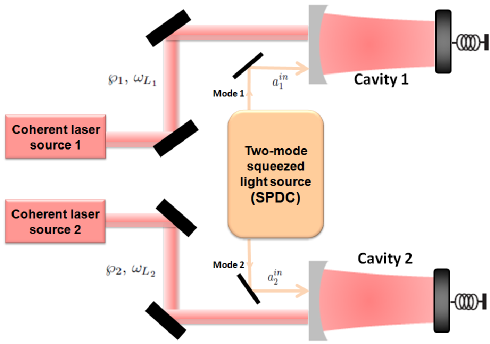
Figure 1: Schematics of two optomechanical Fabry-Perot cavities coupled to a two-mode squeezed light from spontaneous parametric down-conversion (SPDC). The $j^{th}$ cavity is pumped by a coherent laser field of power ${\wp}_{j}$ and frequency $\omega_{L_{j}}$ for $j=1,2$. We will consider a single mechanical mode of the $j^{th}$ movable mirror only, which can be modeled as an harmonic oscillator with frequency $\omega_{\mu_{j}}$, a damping rate $\gamma_{j}$ and an effective mass $m_{\mu_{j}}$. $a_{j}^{in}$ is the $j^{th}$ noise operator corresponding to the $j^{th}$ squeezed mode.

We consider two Fabry-Perot cavities in Fig. 1, where each cavity is composed by two mirrors. The first one is fixed and partially transmitting. The second is movable and perfectly reflecting. As depicted in Fig. 1, the $j^{th}$ cavity is pumped by coherent laser field with the input power ${\wp}_{j}$, phase $\varphi_{j}$ and frequency $\omega_{L_{j}}$. In addition, the two cavities are also pumped by two-mode squeezed light produced for example by spontaneous parametric down-conversion source (SPDC) [29]. The first (respectively, the second) squeezed mode is sent towards the first (second) cavity. Finally, the $j^{th}$ movable mirror modeled as a quantum mechanical harmonic oscillator [30] has an effective mass $m_{\mu_{j}}$, a mechanical damping rate $\gamma_{j}$ and oscillates at frequency denoted by $\omega_{\mu_{j}}$.

2.2 The Hamiltonian

In a frame rotating at the frequency of the lasers, the Hamiltonian of the two optomechanical cavities reads ( $\hbar=1$) [31]:

$$H=\sum_{j=1}^{2}\left[\left(\omega_{c_{j}}-\omega_{L_{j}}\right)a_{j}^{{\dagger}}a_{j}+\omega_{\mu_{j}}b_{j}^{{\dagger}}b_{j}+g_{j}a_{j}^{{\dagger}}a_{j}(b_{j}^{{\dagger}}+b_{j})+\varepsilon_{j}(e^{i\varphi_{j}}a_{j}^{{\dagger}}+e^{-i\varphi_{j}}a_{j})\right].$$ (1)

where $b_{j},b_{j}^{{\dagger}}$ are the annihilation and creation operators associated with the mechanical mode describing the mirror $j$ (for $j=1,2$). They satisfy the usual commutation relations $[b_{j},b_{k}^{{\dagger}}]=\delta_{jk}$ (for $j,k=1,2$). As we shall mainly be concerned in Sec. 3 with the quantum correlations between the mechanical modes, we will refer to the first mode as Alice and to the second mode as Bob. Moreover, $a_{j}$ and $a_{j}^{{\dagger}}$ are the annihilation and creation operators of the $j^{th}$ optical cavity mode. They satisfy also the usual commutation $[a_{j},a_{k}^{{\dagger}}]=\delta_{jk}$. The optomechanical single-photon coupling rate $g_{j}$ between the $j^{th}$ mechanical mode and its corresponding optical cavity mode is given by $g_{j}=\left(\omega_{c_{j}}/l_{j}\right)\sqrt{\hbar/m_{\mu_{j}}\omega_{\mu_{j}}}$ where $l_{j}$ is the $j^{th}$ cavity length. The coupling strength between the $j^{th}$ external laser and its corresponding cavity field is defined by $\varepsilon_{j}=\sqrt{2\kappa_{j}{\wp}_{j}/\hbar\omega_{L_{j}}}$ , $\kappa_{j}$ being the energy decay rate of the $j^{th}$ cavity.

2.3 Quantum Langevin equation

In the Heisenberg picture, the dynamics of the $j^{th}$ mechanical and optical mode variables is completely described by the following set of nonlinear quantum Langevin equations:

$$\partial_{t}b_{j} = -\left(\gamma_{j}/2+i\omega_{\mu_{j}}\right)b_{j}-ig_{j}a_{j}^{{\dagger}}a_{j}+\sqrt{\gamma_{j}}b_{j}^{in},$$ (2)

$$\partial_{t}a_{j} = -\left(\kappa_{j}/2-i\Delta_{j}\right)a_{j}-ig_{j}a_{j}(b_{j}^{{\dagger}}+b_{j})-i\varepsilon_{j}e^{i\varphi_{j}}+\sqrt{\kappa_{j}}a_{j}^{in},$$ (3)

where $\Delta_{j}=\omega_{L_{j}}-\omega_{c_{j}}$ is the $j^{th}$ laser detuning [32] with $j=1,2$. Moreover, $b_{j}^{in}$ is the $j^{th}$ random Brownian operator, with zero mean value ($\langle b_{j}^{in}\rangle=0$), describing the coupling of the $j^{th}$ movable mirror with its own environment. In general, $b_{j}^{in}$ is not $\delta$-correlated [33]. However, quantum effects are reached only using oscillators with a large mechanical quality factor $\mathcal{Q}=\omega_{\mu}/\gamma\gg 1$, which allows us to recover the Markovian process. In this limit, we have the following nonzero time-domain correlation functions [33, 34]:

$$\langle b_{j}^{in{\dagger}}(t)b_{j}^{in}(t^{\prime})\rangle = n_{\mathrm{th,}j}\delta(t-t^{\prime}),$$ (4)

$$\langle b_{j}^{in}(t)b_{j}^{in{\dagger}}(t^{\prime})\rangle = (n_{\mathrm{th,}j}+1)\delta(t-t^{\prime}),$$ (5)

where $n_{\mathrm{th,}j}=\left[\exp(\hbar\omega_{\mu_{j}}/k_{B}T_{j})-1\right]^{-1}$ is the mean thermal photon number, $T_{j}$ is the temperature of the $j^{th}$ mirror environment and $k_{B}$ is the Boltzmann constant. Another kind of noise affecting the system is the $j^{th}$ input squeezed light noise operator $a_{j}^{in}$ with zero mean value ($\langle a_{j}^{in}\rangle=0$). They have the following non-zero correlation properties [35, 36]:

$$\langle\delta a_{j}^{in^{{\dagger}}}(t)\delta a_{j}^{in}(t^{\prime})\rangle = N\delta(t-t^{\prime})\text{ \ for \ \ }j=1,2,$$ (6)

$$\langle\delta a_{j}^{in}(t)\delta a_{j}^{in^{{\dagger}}}(t^{\prime})\rangle = (N+1)\delta(t-t^{\prime})\text{ for \ \ }j=1,2,$$ (7)

$$\langle\delta a_{j}^{in}(t)\delta a_{k}^{in}(t^{\prime})\rangle = Me^{-i\omega_{\mu}(t+t^{\prime})}\delta(t-t^{\prime})\text{ \ for \ }j\neq k=1,2,$$ (8)

$$\langle\delta a_{j}^{in^{{\dagger}}}(t)\delta a_{k}^{in^{{\dagger}}}(t^{\prime})\rangle = Me^{i\omega_{\mu}(t+t^{\prime})}\delta(t-t^{\prime})\text{\ for \ }j\neq k=1,2,$$ (9)

where $N=\mathrm{sinh}^{\mathrm{2}}r$, $M=\mathrm{sinh}r\mathrm{cosh}r$, $r$ being the squeezing parameter (we have assumed that $\omega_{\mu_{1}}=\omega_{\mu_{2}}=\omega_{\mu}$).

2.4 Linearization of quantum Langevin equations

Due to the nonlinear nature of the radiation pressure, the coupled nonlinear quantum Langevin equations (2)-(3) are in general not solvable analytically. To obtain analytical solution to these equations, we adopt the linearization approach discussed in [37, 38]. We decompose each operator ($a_{j}$ and $b_{j}$ for $j=1,2$) into two parts, i.e., sum of its mean value and a small fluctuation with zero mean value. Thus, $\mathcal{O}_{j}=\langle\mathcal{O}_{j}\rangle+\delta\mathcal{O}_{j}=\mathcal{O}_{js}+\delta\mathcal{O}_{j}$ (with $\mathcal{O}_{j}\equiv a_{j},b_{j}$). The mean values $b_{js}$ and $a_{js}$ are obtained by setting the time derivatives to zero and factorizing the averages in Eqs. (2) and (3). Therefore, one gets

$$\langle a_{j}\rangle=a_{js}=\frac{-i\varepsilon_{j}e^{i\varphi_{j}}}{\kappa_{j}/2-i\Delta_{j}^{\prime}}\text{ \ \ \ and \ \ \ }\langle b_{j}\rangle=b_{js}=\frac{-ig_{j}\left|a_{js}\right|^{2}}{\gamma_{j}/2+i\omega_{\mu_{j}}},\qquad$$ (10)

where $\Delta_{j}^{\prime}$ $=$ $\Delta_{j}$ $-g_{j}(b_{js}^{\ast}+b_{js})$ is the $j^{th}$ effective cavity detuning including the radiation pressure effects [32, 39]. To simplify further our purpose, we assume that the double-cavity system is intensely driven ($\left|a_{js}\right|\gg 1$, for $j=1,2$). This assumption can be realized considering lasers with a large input power $\wp_{j}$ [40]. Consequently, the nonlinear terms $\delta a_{j}^{{\dagger}}\delta a_{j}$, $\delta a_{j}\delta b_{j}$ and $\delta a_{j}\delta b_{j}^{{\dagger}}$ can be safely neglected. Hence, we obtain:

$$\delta\dot{b}_{j} = -\left(\gamma_{j}/2+i\omega_{\mu_{j}}\right)\delta b_{j}+G_{j}\left(\delta a_{j}-\delta a_{j}^{{\dagger}}\right)+\sqrt{\gamma_{j}}b_{j}^{in},$$ (11)

$$\delta\dot{a}_{j} = -\left(\kappa_{j}/2-i\Delta_{j}^{\prime}\right)\delta a_{j}-G_{j}\left(\delta b_{j}^{{\dagger}}+\delta b_{j}\right)+\sqrt{\kappa_{j}}\delta a_{j}^{in},$$ (12)

where $G_{j}$ $=g_{j}\left|a_{js}\right|$ is the $j^{th}$ light-enhanced optomechanical coupling in the linearized regime [32]. It is given by:

$$G_{j}=\frac{\omega_{c_{j}}}{l_{j}}\sqrt{\frac{2\kappa_{j}\wp_{j}}{m_{\mu_{j}}\omega_{\mu}\omega_{L_{j}}\left(\left(\frac{\kappa_{j}}{2}\right)^{2}+\left(\Delta_{j}^{\prime}\right)^{2}\right)}}.$$ (13)

Notice that the Eqs. (11) and (12) have been obtained by setting $a_{js}=-i\left|a_{js}\right|$ or equivalently to choose the phase $\varphi_{j}$ of the $j^{th}$ input laser field to be $\varphi_{j}=-\arctan(2\Delta_{j}^{\prime}/\kappa_{j})$. Now, we introduce the operators $\delta\tilde{b}_{j}$ and $\delta\tilde{a}_{j}$ defined by $\delta b_{j}=\delta\tilde{b}_{j}e^{-i\omega_{\mu}t}$ and $\delta a_{j}=\delta\tilde{a}_{j}e^{i\Delta_{j}^{\prime}t}$. Using the Eqs. (11) and (12), we obtain:

$$\delta\dot{\tilde{b}}_{j} = -\frac{\gamma_{j}}{2}\delta\tilde{b}_{j}\ +G_{j}\left(\delta\tilde{a}_{j}e^{i\left(\Delta_{j}^{\prime}+\omega_{\mu}\right)t}-\delta\tilde{a}_{j}^{{\dagger}}e^{-i\left(\Delta_{j}^{\prime}-\omega_{\mu}\right)t}\right)+\sqrt{\gamma_{j}}\tilde{b}_{j}^{in},$$ (14)

$$\delta\dot{\tilde{a}}_{j} = -\frac{\kappa_{j}}{2}\delta\tilde{a}_{j}-G_{j}\left(\delta\tilde{b}_{j}e^{-i\left(\Delta_{j}^{\prime}+\omega_{\mu}\right)t}+\delta\tilde{b}_{j}^{{\dagger}}e^{-i\left(\Delta_{j}^{\prime}-\omega_{\mu}\right)t}\right)+\sqrt{\kappa_{j}}\delta\tilde{a}_{j}^{in}.$$ (15)

Next, we assume that the two cavities are driven at the red sideband ($\Delta_{j}^{\prime}=-\omega_{\mu}$ for $j=1,2$) which corresponds to the quantum states transfer regime [27, 41]. We note also that, in the resolved-sideband regime where the mechanical frequency $\omega_{\mu}$ of the movable mirror is larger than the $j^{th}$ cavity decay rate $\kappa_{j}$ ($\omega_{\mu}\gg\kappa_{1}$, $\kappa_{2}$), one can use the rotating wave approximation (RWA) [32, 42], allowing us to ignore terms rotating at $\pm 2\omega_{\mu}$ in equations (14) and (15). Then, one gets

$$\quad\delta\dot{\tilde{b}}_{j} = -\frac{\gamma_{j}}{2}\delta\tilde{b}_{j}+G_{j}\delta\tilde{a}_{j}+\sqrt{\gamma_{j}}\tilde{b}_{j}^{in},$$ (16)

$$\delta\dot{\tilde{a}}_{j} = -\frac{\kappa_{j}}{2}\delta\tilde{a}_{j}-G_{j}\delta\tilde{b}_{j}+\sqrt{\kappa_{j}}\delta\tilde{a}_{j}^{in}.$$ (17)

2.5 The adiabatic elimination of the optical modes

Being interested only in the quantum correlations between two mechanical modes, the optimal regime for quantum fluctuations transfer from the two-mode squeezed light to the two movable mirrors is achieved when the optical cavities modes adiabatically follow the mechanical modes, which corresponds to the situation where the mirrors have a large mechanical quality factor and weak effective optomechanical coupling ($\kappa_{j}\gg G_{j},$ $\gamma_{j}$) [43]. In this way, inserting the steady state solution of (17) into (16), we obtain a simple description for the two mechanical modes. Then, the $j^{th}$ mirror dynamics reduces to:

$$\delta\dot{\tilde{b}}_{j}=-\frac{\Gamma_{j}}{2}\delta\tilde{b}_{j}+\sqrt{\gamma_{j}}\tilde{b}_{j}^{in}+\sqrt{\Gamma_{\mathrm{a}_{j}}}\delta\tilde{a}_{j}^{in}=-\frac{\Gamma_{j}}{2}\delta\tilde{b}_{j}+\tilde{F}_{j}^{in},$$ (18)

where $\Gamma_{\mathrm{a}_{j}}=4G_{j}^{2}/\kappa_{j}$ is the effective relaxation rate induced by radiation pressure [44], $\Gamma_{j}=$ $\Gamma_{\mathrm{a}_{j}}+\gamma_{j}$ and $\tilde{F}_{j}^{in}=\sqrt{\gamma_{j}}\tilde{b}_{j}^{in}+\sqrt{\Gamma_{\mathrm{a}_{j}}}\delta\tilde{a}_{j}^{in}$. Defining the mechanical fluctuation quadratures, and their corresponding Hermitian input noise operators:

$$\delta\tilde{q}_{j} = (\delta\tilde{b}_{j}^{\dagger}+\delta\tilde{b}_{j})/\sqrt{2},\quad\delta\tilde{p}_{j}=i(\delta\tilde{b}_{j}^{\dagger}-\delta\tilde{b}_{j})/\sqrt{2},$$ (19)

$$\tilde{F}_{q_{j}}^{in} = (\tilde{F}_{j}^{in,{\dagger}}+\tilde{F}_{j}^{in})/\sqrt{2},\qquad\tilde{F}_{p_{j}}^{in}=i(\tilde{F}_{j}^{in,{\dagger}}-\tilde{F}_{j}^{in})/\sqrt{2},$$ (20)

the linearized quantum Langevin equations can be written in the following compact matrix form [45]:

$$\dot{u}(t)=Su(t)+n(t),$$ (21)

where $S=\mathrm{diag}(-\frac{\Gamma_{1}}{2},-\frac{\Gamma_{1}}{2},-\frac{\Gamma_{2}}{2},-\frac{\Gamma_{2}}{2})$, $u(t)^{\mathrm{T}}=(\delta\tilde{q}_{1},\delta\tilde{p}_{1},\delta\tilde{q}_{2},\delta\tilde{p}_{2})$ and $n(t)^{\mathrm{T}}=(\tilde{F}_{q_{1}}^{in},\tilde{F}_{p_{1}}^{in},\tilde{F}_{q_{2}}^{in},\tilde{F}_{p_{2}}^{in})$. The system is stable only if the real parts of all the eigenvalues of the drift matrix $S$ are negative, which is fully verified according to the form of the matrix $S$. Such stability is guaranteed by the fact that both pumps drive the resonators on the red sideband. Therefore, the use of the Routh-Hurwitz criterion [46] is without interest. Nonetheless since we have linearized the dynamics and the noises are zero-mean quantum Gaussian noises, fluctuations in the stable regime will also evolve to an asymptotic zero-mean Gaussian state. It follows that the state of the system is completely described by the correlation matrix $V(t)$ of elements:

$$V_{ii^{\prime}}(t)=\frac{1}{2}(\langle u_{i}(t)u_{i^{\prime}}(t)+u_{i^{\prime}}(t)u_{i}(t)\rangle).$$ (22)

Using Eqs. (21) and (22), the matrix $V(t)$ satisfies the following evolution equation [45]:

$$\frac{d}{dt}V(t)=SV(t)+V(t)S^{\mathrm{T}}+D,$$ (23)

where $D$ is the noise correlation matrix defined by $D_{kk^{\prime}}\delta(t-t^{\prime})=(\langle n_{k}(t)n_{k^{\prime}}(t^{\prime})+n_{k^{\prime}}(t^{\prime})n_{k}(t)\rangle)/2$. Utilizing the correlation properties of the noise operators given by the set of equations [(4)-(9)], we obtain:

$$D=\left(\begin{array}[]{cccc}\ D_{11}&0&D_{13}&0\\ 0&\ \ D_{22}&0&D_{24}\\ D_{13}&0&\ D_{33}&0\\ 0&D_{24}&0&D_{44}\end{array}\right),$$ (24)

where $D_{11}\ \ =D_{22}=\Gamma_{\mathrm{a}_{1}}\left(N+1/2\right)+\gamma_{1}\left(n_{\mathrm{th,}1}+1/2\right)$, $D_{33}=D_{44}=\Gamma_{\mathrm{a}_{2}}\left(N+1/2\right)+\gamma_{2}\left(n_{\mathrm{th,}2}+1/2\right)$ and $D_{13}\ =-D_{24}=M\sqrt{\Gamma_{\mathrm{a}_{1}}\Gamma_{\mathrm{a}_{2}}}$. The equation (23) is an ordinary linear differential equation and can be solved straightforwardly. The corresponding solution can be written as:

$$V(t)=\left(\begin{array}[]{cccc}v_{11}(t)&0&v_{13}(t)&0\\ 0&v_{22}(t)&0&v_{24}(t)\\ v_{13}(t)&0&v_{33}(t)&0\\ 0&v_{24}(t)&0&v_{44}(t)\end{array}\right)\equiv\left(\begin{array}[]{cc}V_{1}(t)&V_{3}(t)\\ V_{3}^{\mathrm{T}}(t)&V_{2}(t)\end{array}\right),$$ (25)

with $V_{1}(t)=\mathrm{diag}(v_{11}(t),v_{22}(t))$, $V_{2}(t)=\mathrm{diag}(v_{33}(t),v_{44}(t))$ and $V_{3}(t)=\mathrm{diag}(v_{13}(t),v_{24}(t))$. We note that $V(t)$ is a real, symmetric and positive definite matrix. The $2\times 2$ matrices $V_{1}(t)$ and $V_{2}(t)$ represent the first and second mechanical mode respectively, while the correlations between them are described by $V_{3}(t)$. Considering identical damping rates ($\gamma_{1}=\gamma_{2}=\gamma$), the explicit expressions of the covariance matrix elements are given by:

$$v_{11}(t) = v_{22}(t)=\frac{(2N+1)\mathcal{C}_{1}+2n_{\mathrm{th,1}}+1}{2(\mathcal{C}_{1}+1)}+\frac{(-2N+1)\mathcal{C}_{1}-2n_{\mathrm{th,1}}+1}{2(\mathcal{C}_{1}+1)}e^{-\gamma(\mathcal{C}_{1}+1)t},$$ (26)

$$v_{33}(t) = v_{44}(t)=\frac{(2N+1)\mathcal{C}_{2}+2n_{\mathrm{th,2}}+1}{2(\mathcal{C}_{2}+1)}+\frac{(-2N+1)\mathcal{C}_{2}-2n_{\mathrm{th,2}}+1}{2(\mathcal{C}_{2}+1)}e^{-\gamma(\mathcal{C}_{2}+1)t},$$ (27)

$$v_{13}(t) = -v_{24}(t)=\frac{2M\sqrt{\mathcal{C}_{1}\mathcal{C}_{2}}}{\mathcal{C}_{1}+\mathcal{C}_{2}+2}\left(1-e^{-\frac{\gamma}{2}(\mathcal{C}_{1}+\mathcal{C}_{2}+2)t}\right),$$ (28)

where $\mathcal{C}_{j}$ is the $j^{th}$ optomechanical cooperativity [47]:

$$\mathcal{C}_{j}=\Gamma_{\mathrm{a}_{j}}/\gamma=4G_{j}^{2}/\gamma\kappa_{j}=\frac{8\omega_{c_{j}}^{2}}{\gamma m_{\mu_{j}}\omega_{\mu}\omega_{L_{j}}l_{j}^{2}}\frac{\ \wp_{j}}{\left[\left(\frac{\kappa_{j}}{2}\right)^{2}+\omega_{\mu}^{2}\right]}.$$ (29)

In the strong optomechanical coupling regime, where $\mathcal{C}_{1,2}\gg 1$ (in the limit of strong coupling $\mathcal{C}_{1,2}\rightarrow 10^{6}$ [48]) and longer time, $v_{11}(t)$, $v_{33}(t)$ and $v_{13}(t)$ reduce respectively to $v_{11}(t)=v_{33}(t)=\frac{1}{2}\mathrm{cosh}(2r)$ and $v_{13}(t)=\frac{1}{2}\mathrm{sinh}(2r)$, meaning that quantum correlations can be governed only by the squeezing degree $r$. Moreover, when either $\mathcal{C}_{1}=0$, $\mathcal{C}_{2}=0$ or $r=0$, we have $v_{13}(t)=v_{24}(t)=0$ or equivalently $\det V_{3}=0$, which corresponds to the Gaussian product states [49], so that the two modes $A$ and $B$ remain separable and consequently, they would be non-steerable in any direction [10]. This is a consequence of the fact that $\det V_{3}<0$ is a necessary condition for a two-mode Gaussian state to be entangled [50]. Therefore, non zero optomechanical coupling and non zero squeezing are necessary conditions to correlate the two separated modes $A$ and $B$. Finally, from Eqs. [(26)-(28)], it is not difficult to show that when $t\rightarrow\infty$ which corresponds to the stationary regime, $v_{11}(\infty)$, $v_{33}(\infty)$ and $v_{13}(\infty)$ coincide respectively with Eqs. (21), (22) and (23) in Ref [51].

3 Gaussian quantum steering and its asymmetry

Now, we are in position to study the dynamics of Gaussian quantum steering and its asymmetry between the two mechanical modes $A$ and $B$. To quantify how much a bipartite Gaussian state with covariance matrix $V(t)$ is steerable, we use the compact formula which has been proposed recently in Ref [10]. Let us start by giving the definition of quantum steerability. Following [4, 10], a bipartite state $\varrho_{AB}$ is steerable from $A$ to $B$ (i.e., Alice can steer Bob’s states) after accomplishing a set of measurements $\mathcal{M}_{A}$ on Alice’s side iff it is not possible for every pair of local observables $R_{A}\in\mathcal{M}_{A}$ on $A$ and $R_{B}$ (arbitrary) on $B$, with respective outcomes $r_{A}$ and $r_{B}$, to express the joint probability as $P(r_{A},r_{B}|R_{A},R_{B},\varrho_{AB})=\sum_{\lambda}\mathcal{P}_{\lambda}\mathcal{P}(r_{A},R_{A}|\lambda)P(r_{B},R_{B}|\varrho_{\lambda})$ [4]. This means that at least one measurement pair $R_{A}$ and $R_{B}$ must violate this expression when $\mathcal{P}_{\lambda}$ is fixed across all measurements [4, 10]. Here $\mathcal{P}_{\lambda}$ and $\mathcal{P}(r_{A},R_{A}|\lambda)$ are probability distributions and $P(r_{B},R_{B}|\varrho_{\lambda})$ is the conditional probability distribution associated to the extra condition of being evaluated on the state $\varrho_{\lambda}$.
A bipartite system of two-mode Gaussian state $\varrho_{AB}$ with covariance matrix $V$ (Eq. (25)) is $A\rightarrow B$ steerable by Alice’s Gaussian measurements, iff the following condition is violated [4]:

$$V+i(0_{A}\oplus\Omega_{B})\geqslant 0,$$ (30)

where $0_{A}$ is a $2\times 2$ null matrix and $\Omega_{B}$ $=\left(\begin{array}[]{cc}0&1\\ -1&0\end{array}\right)$ is the $B$-mode symplectic matrix [10]. Henceforth, a violation of the condition (30) is necessary and sufficient for the Gaussian $A\rightarrow B$ steerability [10].
A computable measure to quantify how much a bipartite two-mode Gaussian state with covariance matrix $V$ (25) is steerable by Gaussian measurements on Alice’s side, is given by [10]:

$$\mathcal{G}^{A\rightarrow B}(V):=\max\{0,-\ln(\bar{\nu}^{B})\},$$ (31)

with $\bar{\nu}^{B}=\sqrt{\det M^{B}}$ the symplectic eigenvalue of the matrix $M^{B}$ written as $M^{B}=V_{2}-V_{3}^{\mathrm{T}}V_{1}^{-1}V_{3}$, where the $2\times 2$ matrices $V_{1}$, $V_{2}$ and $V_{3}$ are defined by Eq. (25).
The Gaussian quantum steering $\mathcal{G}^{A\rightarrow B}$ vanishes when the state described by the covariance matrix $V$ (25) is nonsteerable by Alice’s measurements, and it generally quantifies the amount by which the condition (30) fails to be fulfilled [10]. With quadratures given by [(19)-(20)] and the covariance matrix (25) expressed in the ordered basis ($\delta\tilde{q}_{1},\delta\tilde{p}_{1},\delta\tilde{q}_{2},\delta\tilde{p}_{2}$), the Gaussian steerability $A\rightarrow B$ given by Eq. (31) takes the following simple form[10]:

$$\mathcal{G}^{A\rightarrow B}=\max\left[0,\frac{1}{2}\ln\frac{\det V_{1}(t)}{4\det V(t)}\right]=\max\left[0,\text{ }-\ln 2\left(v_{33}(t)-\frac{(v_{13}(t))^{2}}{v_{11}(t)}\right)\right],$$ (32)

where $v_{11}(t),v_{33}(t)$ and $v_{13}(t)$ are explicitly given by Eqs. [(26)-(28)]. Similarly, a corresponding measure of the Gaussian $B\rightarrow A$ steerability can be obtained by swapping the roles of $A$ and $B$ in (32). One gets:

$$\mathcal{G}^{B\rightarrow A}=\max\left[0,\frac{1}{2}\ln\frac{\det V_{2}(t)}{4\det V(t)}\right]=\max\left[0,\text{ }-\ln 2\left(v_{11}(t)-\frac{(v_{13}(t))^{2}}{v_{33}(t)}\right)\right].$$ (33)

The explicit analytical expressions of $\mathcal{G}^{A\rightarrow B}$ and $\mathcal{G}^{B\rightarrow A}$ are too cumbersome and will not be reported here. It is well known that quantum entanglement is a symmetric property shared between two systems $A$ and $B$ without specification of direction, i.e., if $A$ is entangled with $B$, $B$ is necessarily entangled with $A$. However, quantum steering is an asymmetric property ,i.e., a quantum state may be steerable from Alice to Bob, but not vice versa [10]. Thus, we shall consider three cases: ($i$) $\mathcal{G}^{A\rightarrow B}=\mathcal{G}^{B\rightarrow A}=0$ as no-way steering, ($ii$) $\mathcal{G}^{A\rightarrow B}>0$ and $\mathcal{G}^{B\rightarrow A}=0$ or $\mathcal{G}^{A\rightarrow B}=0$ and $\mathcal{G}^{B\rightarrow A}>0$ as one-way steering, and finally ($iii$) $\mathcal{G}^{A\rightarrow B}>0$ and $\mathcal{G}^{B\rightarrow A}>0$ as two-way steering. In order to check how asymmetric can the steerability be between the mechanical modes $A$ and $B$, we use the Gaussian steering asymmetry $\mathcal{G}_{AB}^{\Delta}$ defined as [10]:

$$\mathcal{G}_{AB}^{\Delta}=\left|\mathcal{G}^{A\rightarrow B}-\mathcal{G}^{B\rightarrow A}\right|.$$ (34)

On the other hand, to compare between quantum steering and entanglement as two different aspects of inseparable quantum correlations, it is more convenient to plot them simultaneously under the same circumstances. To accomplish this, we use the Gaussian Rényi-$2$ entropy [20, 21] as an appropriate measure to quantify entanglement between the two modes $A$ and $B$ [10].
In quantum information theory, an interesting family of additive entropies is represented by Rényi-$\alpha$ entropies [52] defined by [20]:

$$\mathcal{S}_{\alpha}\mathcal{(\varrho)=(}1-\alpha\mathcal{)}^{-1}\ln\mathrm{Tr}\left(\varrho^{\alpha}\right).$$ (35)

In particular, when $\alpha\rightarrow 1,$ the entropies given by Eq. (35) reduce to the von Neumann entropy
$\mathcal{S(\varrho)=}-\mathrm{Tr}\left(\varrho\ln\varrho\right)$ [20], which quantifies the degree of information contained in a quantum state $\mathcal{\varrho}.$ While, for $\alpha=2$, we obtain the Gaussian Rényi-2 entropy defined by [20]:

$$\mathcal{S}_{2}\mathcal{(\varrho)=}-\ln\mathrm{Tr}\left(\varrho^{2}\right).$$ (36)

It has been shown in [20], that Rényi-2 entropy provides a natural measure of information for any multimode Gaussian state of quantum harmonic systems. Importantly, it has been demonstrated also in [20] that for all Gaussian states, Rényi-2 entropy satisfies the strong subadditivity inequality, i.e., $\mathcal{S}_{2}\left(\mathcal{\varrho}_{AB}\right)+\mathcal{S}_{2}\left(\mathcal{\varrho}_{BC}\right)\geqslant\mathcal{S}_{2}\left(\mathcal{\varrho}_{ABC}\right)+\mathcal{S}_{2}\left(\mathcal{\varrho}_{B}\right)$, which made it possible to define measures of Gaussian Rényi-2 entanglement [21, 53] and discord-like quantum correlations [49, 54].
For generally mixed two-mode Gaussian states $\mathcal{\varrho}_{AB}$, the Rényi-2 entanglement measure $\mathcal{E}_{2}\mathcal{(\varrho}_{A:B}\mathcal{)\equiv E}_{2}$, defined by Eq. (36), admits an unclosed cumbersome formula which will not be reported here [20, 21]. However, for relevant subclasses of states including symmetric states [55], squeezed thermal states [49], and so-called GLEMS-Gaussian states of partial minimum uncertainty [21], closed formulas of Gaussian Rényi-2 entanglement have been found [21]. The covariance matrix $V(t)$ (25) is in the so-called standard form [50] and characterized by $v_{13}(t)=-v_{24}(t)$ (28) which corresponds to the squeezed thermal states STS [49]. Therefore, the Gaussian Rényi-2 entanglement measure $\mathcal{E}_{2}$, admits the following expression [20, 21]:

$$\mathcal{E}_{2}=\frac{1}{2}\ln\left[h(s,d,g)\right],$$ (37)

with:

$$h(s,d,g)=\left\{\begin{array}[]{c}1\text{ \ \ \ \ \ \ \ \ \ \ \ \ \ \ \ \ \ \ \ \ \ \ \ \ \ \ \ \ \ \ \ \ \ \ \ \ \ \ iff\ \ \ \ \ \ \ \ \ }4g\geqslant 4s-1,\\ \left[\frac{(4g+1)s-\sqrt{\left[(4g-1)^{2}-16d^{2}\right]\left[s^{2}-d^{2}-g\right]}}{4(d^{2}+g)}\right]^{2}\text{ \ iff \ \ \ \ }4|d|+1\leq 4g<4s-1,\end{array}\right.$$ (38)

where $s=\frac{1}{2}(v_{11}(t)+v_{33}(t)),$ $d=\frac{1}{2}(v_{11}(t)-v_{33}(t))$ and $g=\left(v_{11}(t)v_{33}(t)-v_{13}^{2}(t)\right)$.

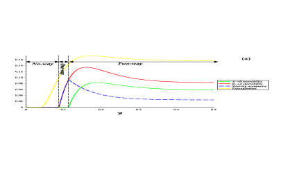
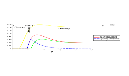
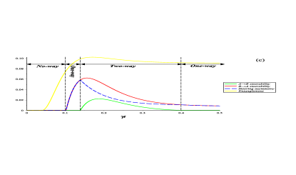
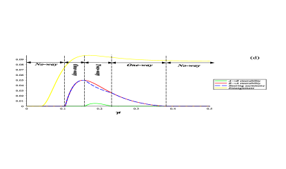
Figure 2: Plot of the Gaussian steering $\mathcal{G}^{A\rightarrow B}$ (green solid line), $\mathcal{G}^{B\rightarrow A}$ (red solid line), the steering asymmetry $\mathcal{G}_{AB}^{\Delta}$ (blue dashed line) and entanglement $\mathcal{E}_{2}$ (yellow solid line) of the two mechanical modes $A$ and $B$ as a function of the scaled time $\gamma t$ for $\mathcal{C}_{1}=15$, $\mathcal{C}_{2}=35$ and $r=1$. The mean thermal photons numbers $n_{\mathrm{th},1}$ and $n_{\mathrm{th},2}$ are fixed as : $n_{\mathrm{th},1}=0.5$ and ${n_{\mathrm{th},2}=1}$ (panel (a)), $n_{\mathrm{th},1}=1$ and $n_{\mathrm{th},2}=0.5$ (panel (b)), $n_{\mathrm{th},1}=1$ and $n_{\mathrm{th},2}=1.2$ (panel (c)) and $n_{\mathrm{th},1}=1$ and $n_{\mathrm{th},2}=1.5$ (panel (d)). Obviously, panels (a) and (b) show that when interchanging the values of $n_{\mathrm{th,}1}$ and $n_{\mathrm{th,}2}$, the Gaussian Rényi-2 entanglement $\mathcal{E}_{2}$ is insensitive to this operation (unlike the steerabilities $\mathcal{G}^{A\rightarrow B}$, $\mathcal{G}^{B\rightarrow A}$), which means that the Gaussian Rényi-2 entanglement is unable to detect the asymmetry shown by the steering criteria (see Eqs. (32)-(33)). This figure shows also that steerable states are strictly inseparable but not necessarily vice versa.

The expressions of $\mathcal{G}^{A\rightarrow B}$, $\mathcal{G}^{B\rightarrow A}$, $\mathcal{G}_{AB}^{\Delta}$ and $\mathcal{E}_{2}$ involve the covariance matrix elements (25) which are expressed in terms of the squeezing parameter $r$, the $j^{th}$ optomechanical cooperativity $\mathcal{C}_{j}$ and the $j^{th}$ mean thermal photons number $n_{\mathrm{th,}j}$. In what follows, we shall consider the case where $n_{\mathrm{th,}1}\neq n_{\mathrm{th,}2}$ and $\mathcal{C}_{1}\neq\mathcal{C}_{2}$ so that the system is not symmetric by swapping the first and the second mode, which is a crucial condition to ensure the Gaussian steering asymmetry. In our simulations, the system parameters have been taken from [56]. The movable mirrors having the mass $\mu_{1,2}=145~{}\mathrm{ng}$ and oscillate at frequency $\omega_{\mu_{1,2}}=2\pi\times 947\times 10^{3}~{}\mathrm{Hz}$ with a mechanical damping rate $\gamma_{1,2}=2\pi\times 140~{}\mathrm{Hz}$. The two cavities have length $l_{1,2}=25~{}\mathrm{\ mm}$, wave length $\lambda_{1,2}=1064~{}\mathrm{nm}$, decay rate $\kappa_{1,2}=2\pi\times 215\times 10^{3}~{}\mathrm{Hz}$, frequency $\omega_{c_{1,2}}=2\pi\times 5.26\times 10^{14}~{}\mathrm{Hz}$ and pumped by laser fields of frequency $\omega_{L_{1,2}}=2\pi\times 2.82\times 10^{14}$ $\mathrm{Hz}$. For the powers of the coherent laser sources, we take $\wp_{1}=5~{}\mathrm{mW}$ and $\wp_{2}=11~{}\mathrm{mW}$ [56]. Next, using the explicit expression of the dimensionless $j^{th}$ optomechanical cooperativity $\mathcal{C}_{j}$ given by Eq. (29), one has $\mathcal{C}_{1}$ $\simeq$ $35$ and $\mathcal{C}_{2}$ $\simeq 15$. Taking the above parameters into account, we find the following sequence of inequalities:

$$\omega_{\mu}\gg\kappa\gg G_{j},$$ (39)

where the parameter $G_{j}$ (for $j=1,2$) is given by Eq. (13). So, in accordance with [24, 32, 40, 42, 57], the condition $\omega_{\mu}\gg\kappa$ justifies the use of the rotating wave approximation. Meanwhile, $\kappa\gg G_{j}$ which is the condition of the weak-coupling regime, allows us the adiabatic elimination of the optical cavities modes [24, 40, 43, 57]. Concerning the environmental parameters (the squeezing parameter $r$ and the thermal occupations $n_{\mathrm{th},1}$ and $n_{\mathrm{th},2}$), we have chosen them of the same order of magnitude as those used in [58].
Fixing the squeezing parameter as $r=1$, Fig. 2 shows the influence of the mean thermal photons numbers $n_{\mathrm{th,}1}$ and $n_{\mathrm{th,}2}$ on the dynamics of the Gaussian steerabilities $\mathcal{G}^{A\rightarrow B}$ and $\mathcal{G}^{B\rightarrow A}$, the steering asymmetric $\mathcal{G}_{AB}^{\Delta}$ and entanglement $\mathcal{E}_{2}$. The mean thermal occupations $n_{\mathrm{th,}1}$ and $n_{\mathrm{th,}2}$ are fixed as : $n_{\mathrm{th,}1}=0.5$, $n_{\mathrm{th,}2}=1$ (panel (a)), $n_{\mathrm{th,}1}=1$, $n_{\mathrm{th,}2}=0.5$ (panel (b)), $n_{\mathrm{th,}1}=1$, $n_{\mathrm{th,}2}=1.2$ (panel (c)) and $n_{\mathrm{th,}1}=1$, $n_{\mathrm{th,}2}=1.5$ (panel (d)). As seen from Fig. 2, $\mathcal{G}^{A\rightarrow B}$, $\mathcal{G}^{B\rightarrow A}$ and $\mathcal{E}_{2}$ have the same time-evolution behavior. Indeed, the initial phase is a period where $\mathcal{G}^{A\rightarrow B}$, $\mathcal{G}^{B\rightarrow A}$ and $\mathcal{E}_{2}$ are zero, exhibiting a time delay before a sudden birth, which is analogous to the superradiance phenomenon. The second phase occurs when the three measures follow a chronological hierarchy and gradual build-up until a maximal value, and finally the third phase occurs when the three measures start to diminish. Moreover, Fig. 2 shows that the influence of the asymmetric values of $n_{\mathrm{th,}1}$ and $n_{\mathrm{th,}2}$ is not only reflected on the time-generation of the steerabilities $\mathcal{G}^{A\rightarrow B}$ and $\mathcal{G}^{B\rightarrow A}$ but also on their time-residence too. Fig. 2 depicts also that steerable states are always entangled as expected, but entangled states are not necessarily steerable, which means that stronger quantum correlations are required for achieving the steering than that for the entanglement. More important, Fig. 2 shows different situations where $\mathcal{G}^{A\rightarrow B}=0$, $\mathcal{G}^{B\rightarrow A}$ $>0$ and $\mathcal{E}_{2}>0$, which witnesses the existence of Gaussian one-way steering, i.e., the states of the two modes $A$ and $B$ are steerable only from $B$ to $A$ even though they are entangled. This behavior constitutes a genuine response to the problem which has been discussed in [4]. In addition, Fig. 2 reveals that the two steerabilities $B\rightarrow A$ and $A\rightarrow B$ are strongly sensitive to the variations of $n_{\mathrm{th,}1}$ and $n_{\mathrm{th,}2}$ than entanglement, and they have a tendency to disappear rapidly when the temperature increases.
Now, fixing the mean thermal photons numbers as $n_{\mathrm{th,}1}=n_{\mathrm{th,}2}=1$, we discuss the dynamics of $\mathcal{G}^{A\rightarrow B}$, $\mathcal{G}^{B\rightarrow A}$ and $\mathcal{E}_{2}$ under influence of the squeezing parameter $r$.

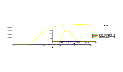
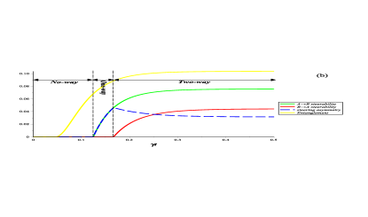
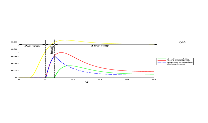
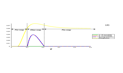
Figure 3: Plot of the Gaussian steering $\mathcal{G}^{A\rightarrow B}$ (green solid line), $\mathcal{G}^{B\rightarrow A}$ (red solid line), the steering asymmetry $\mathcal{G}_{AB}^{\Delta}$ (blue dashed line) and entanglement $\mathcal{E}_{2}$ (yellow solid line) of the two mechanical modes $A$ and $B$ as a function of the scaled time $\gamma t$ for $\mathcal{C}_{1}=15$ and $\mathcal{C}_{2}=35$. We used $n_{\mathrm{th},1}=n_{\mathrm{th},2}=1$ as values of the mean thermal photons numbers. The squeezing parameter $r$ is fixed as : $r=0.1$ (panel (a)), $r=0.5$ (panel (b)), $r=1$ (panel (c)) and $r=1.1$ (panel (d)) and $r=1.7$ in the inset. Panel (d) shows a situation where the states of the two mechanical modes are entangled (for $\gamma t>0.05$); nevertheless they are straightforwardly steerable only in one direction (from $B\rightarrow A$), which reflects genuinely the asymmetry of quantum correlations between the modes $A$ and $B$. As shown also in panel (a) and in the inset, entangled states are not necessarily steerable, whereas steerable states are always entangled as depicted in the panels (b), (c) and (d).

Firstly, like the results which have been presented in Fig. 2, we see from Fig. 3 that steerable states are always entangled, whereas entangled states are not in general steerable. Moreover, Fig. 3 shows that with gradual increase of the squeezing parameter $r$ : $r=0.1$ (panel (a)), $r=0.5$ (panel (b)), $r=1$ (panel (c)), $r=1.1$ (panel (d)) and $r=1.7$ (in the inset), the squeezing has two opposite effects (enhancement and degradation) on the behavior of $\mathcal{G}^{A\rightarrow B}$, $\mathcal{G}^{B\rightarrow A}$ and $\mathcal{E}_{2}$. The enhancement is due to the fact that the photon number in the two cavities increases which enhances the optomechanical coupling by means of radiation pressure and consequently leads to robust quantum correlations. However, in the degradation period, the input thermal noise affecting each cavity becomes important and more aggressive, causing the quantum correlation degradation. This double-effect of the two-mode squeezed light can be understood based on the fact that the reduced state of a two-mode squeezed light is a thermal state having an average number of photons proportional to the squeezing parameter $r$ [36]. On the other hand, comparing with entanglement, it can be clearly seen from Fig. 3 that quantum steering is considerably sensitive to thermal noise induced by the gradual increasing of $r$. Fig. 3(d) shows an interesting situation where the states of the two mechanical modes $A$ and $B$ are entangled (for $\gamma t>0.05$); nevertheless they are steerable only in one direction (from $B\rightarrow A$), which reflects genuinely the asymmetry of quantum correlations. Such a property translates the fact that Alice and Bob can perform exactly the same Gaussian measurements on their part of the entangled system, but obtain different results. This can be explained by the asymmetry introduced in the system and also by the definition of quantum steering in terms of the EPR paradox [11, 10]. Finally, all results depicted in Figs. 2 and 3 show that the Gaussian quantum steering is always upper bounded by the Gaussian Rényi-2 entanglement $\mathcal{E}_{2}$. Moreover, the steering asymmetry $\mathcal{G}_{AB}^{\Delta}$ (see the blue dashed-lines in Figs. 2 and 3) is always less than $\ln 2$, it is maximal when the state is nonsteerable in one way ($\mathcal{G}^{A\rightarrow B}>0$ and $\mathcal{G}^{B\rightarrow A}=0$ or $\mathcal{G}^{A\rightarrow B}=0$ and $\mathcal{G}^{B\rightarrow A}>0$) and it decreases with increasing steerability in either way, which is consistent with the literature [10].

4 Conclusions

Using the criterion proposed in [10], dynamical Gaussian quantum steering and its asymmetry of two mixed mechanical modes $A$ and $B$ have been studied. A specific attention has been devoted to the dynamics of the Gaussian one-way steerability. For this, a double-cavity optomechanical system coupled to a common two-mode squeezed light has been employed. We worked in the resolved sideband regime with high quality factor mechanical oscillators. Eliminating adiabatically the optical cavities modes, we have derived the explicit time-dependent expression of the covariance matrix (Eq. (25)) fully describing the mechanical fluctuations. In this way, we have shown that it is possible to generate dynamical Gaussian quantum steering via a quantum fluctuations transfer from the two-mode squeezed light to the mechanical modes, whereas by an appropriate choice of the environmental parameters (thermal occupations $n_{\mathrm{th},1}$, $n_{\mathrm{th},2}$ and squeezing $r$), Gaussian one-way steering can be observed in different scenarios : (i) Gaussian one-way steering has been detected from $A\rightarrow B$ (see Fig. 3(b)) as well as from $B\rightarrow A$ (see Fig. 2 and Figs. 3(c)-3(d)), (ii) it has been observed from $B\rightarrow A$ during two periods (see Figs. 2(c)-2(d)), and finally (iii) Gaussian one-way steering has occurred without two-way steering behavior (see Fig. 3(d)). We have shown also that in some circumstances which are governed by thermal effects, one can observe the situation where the two mechanical modes are entangled, yet are straightforwardly steerable only in one direction (see Fig. 3(d)), which reflects genuinely the asymmetry of quantum correlations. On the other hand, we have numerically compared the Gaussian steering of the two mechanical modes $A$ and $B$ with their corresponding entanglement. Using the Gaussian Rényi-2 entropy as a measure of entanglement, we showed that Gaussian steering is strongly sensitive to the thermal effects than entanglement and always upper bounded by the Gaussian Rényi-2 entanglement $\mathcal{E}_{2}$. Furthermore, we have found that the steering asymmetry $\mathcal{G}_{AB}^{\Delta}$ is always less than $\ln 2$, it is maximal when the state is nonsteerable in one way, and it decreases with increasing steerability in either way, which is consistent with the literature [10].
So, we believe that a Fabry-Perot double-cavity optomechanical system can be of immediate practical interest in the investigation of Gaussian quantum steering and its asymmetry between two mechanical modes. In addition, the transfer of quantum fluctuations from two-mode squeezed light to mechanical motions can be exploited to gain quantum advantages in implementing long distance quantum protocols. We note also that an equivalent scheme can be considered to study Gaussian steering between optical modes which may open a new perspective in the context of quantum key distribution and in quantum information science in general [17, 18, 19]. Finally, it will be interesting to investigate stationary Gaussian one-way steering in a double-cavity optomechanical system using the criterion of Kogias et al [10]. We hope to report on this issue in a forthcoming work.

Author Contributions

The authors contributed equally to this work.

References

- [1] A. Einstein, B. Podolsky, and N. Rosen, Phys. Rev. 47, 777 (1935).
- [2] E. Schrödinger, Naturwiss. 23, 807 (1935); R. Horodecki, P. Horodecki, M. Horodecki, and K. Horodecki, Rev. Mod. Phys. 81, 865 (2009).
- [3] J. S. Bell, Physics 1, 195 (1964); J. F. Clauser, M. A. Horne, A. Shimony and R. A. Holt, Phys. Rev. Lett. 23, 880 (1969).
- [4] H. M. Wiseman, S. J. Jones, and A. C. Doherty, Phys. Rev. Lett. 98, 140402 (2007).
- [5] S. Wollmann, N. Walk, A. J. Bennet, H. M. Wiseman, and G. J. Pryde, Phys. Rev. Lett. 116, 160403 (2016).
- [6] A. Aspect, P. Grangier, and G. Roger, Phys. Rev. Lett. 49, 91 (1982); H. Nha, H. J. Carmichael, Phys. Rev. Lett. 93, 020401 (2004); A. Acin, T. Durt, N. Gisin, J. I. Latorre, Phys. Rev. A 65, 052325 (2002); N. Brunner, D. Cavalcanti, S. Pironio, V. Scarani, S. Wehner, Rev. Mod. Phys. 86, 419 (2014).
- [7] M. D. Reid, P. D. Drummond, W. P. Bowen, E. G. Cavalcanti, P. K. Lam, H. A. Bachor, U. L. Andersen, and G. Leuchs, Rev. Mod. Phys. 81, 1727 (2009).
- [8] E. Schrödinger, Math. Proc. Cambridge Philos. Soc. 31, 555 (1935); E. Schrödinger, Proc. Camb. Phil. Soc. 32, 446 (1936).
- [9] K. Sun, J. -S. Xu, X. -J. Ye, Y. -C. Wu, J. -L. Chen, C. -F. Li, and G. -C. Guo, Phys. Rev. Lett. 113, 140402 (2014).
- [10] I. Kogias, A. R. Lee, S. Ragy, and G. Adesso, Phys. Rev. Lett. 114, 060403 (2015).
- [11] M. D. Reid, Phys. Rev. A 40, 913 (1989).
- [12] Z. Y. Ou, S. F. Pereira, H. J. Kimble, and K. C. Peng, Phys. Rev. Lett. 68, 3663 (1992).
- [13] D. J. Saunders, S. J. Jones, H. M. Wiseman and G. J. Pryde, Nat. Phys. 6, 845 (2010); D. H. Smith, G. Gillett, M. P. de Almeida, C. Branciard, A. Fedrizzi, T. J. Weinhold, A. Lita, B. Calkins, T. Gerrits, H. M. Wiseman, S. W. Nam and A. G. White, Nature Commun. 3, 625 (2012); J. Chan, T. P. M. Alegre, A. H. S. -Naeini, J. T. Hill, A. Krause, S. Gröblacher, M. Aspelmeyer and O. Painter, Nature 478, 89 (2011); J. D. Teufel, D. Li, M. S. Allman, K. Cicak, A. J. Sirois, J. D. Whittaker and R. W. Simmonds, Nature 471, 204 (2011); E. Verhagen, S. Deléglise, S. Weis, A. Schliesser and T. J. Kippenberg, Nature 482, 63 (2012).
- [14] S. L. W. Midgley, A. J. Ferris, and M. K. Olsen, Phys. Rev. A 81, 022101 (2010); V. Händchen, T. Eberle, S. Steinlechner, A. Samblowski, T. Franz, R. F. Werner and R. Schnabel, Nat. Photonics 6, 596 (2012); Q. Y. He and M. D. Reid, Phys. Rev. A 88, 052121 (2013); H. Tan, X. Zhang, and G. Li, Phys. Rev. A 91, 032121 (2015).
- [15] E. G. Cavalcanti, Q. Y. He, M. D. Reid, and H. M. Wiseman, Phys. Rev. A 84, 032115 (2011); S. P. Walborn, A. Salles, R. M. Gomes, F. Toscano, and P. H. Souto Ribeiro, Phys. Rev. Lett. 106, 130402 (2011); M. K. Olsen and J. F. Corney, Phys. Rev. A 87, 033839 (2013); M. K. Olsen, Phys. Rev. A 88, 051802(R) (2013); J. Bowles, T. Vértesi, M. T. Quintino, and N. Brunner, Phys. Rev. Lett. 112, 200402 (2014); M. K. Olsen, J. Opt. Soc. Am. B 32, A15 (2015); Q. Y. He, Q. H. Gong, and M. D. Reid, Phys. Rev. Lett. 114, 060402 (2015); I. Kogias and G. Adesso, J. Opt. Soc. Am. B 32, A27 (2015); J. Wang, H. Cao, J. Jing, and H. Fan, Phys. Rev. D 93, 125011 (2016).
- [16] B. Wittmann, S. Ramelow, F. Steinlechner, N. K. Langford, N. Brunner, H. M. Wiseman, R. Ursin and A. Zeilinger, New J. Phys. 14, 053030 (2012); S. Armstrong, M. Wang, R. Y. Teh, Q. Gong, Q. He, J. Janousek, H. -A. Bachor, M. D. Reid and P. K. Lam, Nat. Phys. 11, 167 (2015); S. Kocsis, M. J. W. Hall, A. J. Bennet, D. J. Saunders and G. J. E. Pryde, Nat. Commun 6, 5886 (2015); A. J. Bennet, D. A. Evans, D. J. Saunders, C. Branciard, E. G. Cavalcanti, H. M. Wiseman, and G. J. Pryde, Phys. Rev. X 2, 031003 (2012).
- [17] C. Branciard, E. G. Cavalcanti, S. P. Walborn, V. Scarani, and H. M. Wiseman, Phys. Rev. A 85, 010301(R) (2012).
- [18] M. D. Reid, Phys. Rev. A 88, 062338 (2013).
- [19] Y. Z. Law, L. P. Thinh, J. -D. Bancal, V. Scarani, J. Phys. A: Math. Theor. 47 424028 (2014).
- [20] G. Adesso, D. Girolami, and A. Serafini, arXiv:1203.5116 [quant-ph]; G. Adesso, D. Girolami, and A. Serafini, Phys. Rev. Lett. 109, 190502 (2012).
- [21] G. Adesso and F. Illuminati, Phys. Rev. A 72, 032334 (2005).
- [22] Q. He and Z. Ficek, Phys. Rev. A 89, 022332 (2014).
- [23] R. Riedinger, S. Hong, R. A. Norte, J. A. Slater, J. Shang, A. G. Krause, V. Anant, M. Aspelmeyer, S. Gröblacher, Nature 530, 313 (2016); T. A. Palomaki, J. D. Teufel, R. W. Simmonds and K. W. Lehnert, Science 342, 710 (2013); M. Ludwig, A. H. S. -Naeini, O. Painter and F. Marquardt, Phys. Rev. Lett 109, 063601 (2012); M. A. Lemonde, N. Didier and A. A. Clerk, Nat Commun 7, 11338 (2016); C. Schäfermeier, H. Kerdoncuff, U. B. Hoff, H. Fu, A. Huck, J. Bilek, G. I. Harris, W. P. Bowen, T. Gehring, and U. L. Andersen, Nat Commun 7, 13628 (2016); S. G. Hofer and K. Hammerer, Phys. Rev. A 91, 033822 (2015); Q. Mu, X. Zhao, and T. Yu, Phys. Rev. A 94, 012334 (2016); F. M. Buters, M. J. Weaver, H. J. Eerkens, K. Heeck, S. de Man, and D. Bouwmeester, Phys. Rev. A 94, 063813 (2016); B. Nair, A. Xuereb, and A. Dantan, Phys. Rev. A 94, 053812 (2016); Y. Yanay, J. C. Sankey, and A. A. Clerk, Phys. Rev. A 93, 063809 (2016); R. A. Norte, J. P. Moura, and S. Gröblacher, Phys. Rev. Lett. 116, 147202 (2016); R. W. Peterson, T. P. Purdy, N. S. Kampel, R. W. Andrews, P. -L. Yu, K. W. Lehnert, and C. A. Regal, Phys. Rev. Lett. 116, 063601 (2016).
- [24] S. G. Hofer, W. Wieczorek, M. Aspelmeyer, and K. Hammerer, Phys. Rev. A 84, 052327 (2011).
- [25] J. Zhang, K. Peng, and S. L. Braunstein, Phys. Rev. A 68, 013808 (2003); M. Paternostro, D. Vitali, S. Gigan, M. S. Kim, C. Brukner, J. Eisert, and M. Aspelmeyer, Phys. Rev. Lett. 99, 250401 (2007); M. Paternostro, L. Mazzola and J. Li, J. Phys. B: At. Mol. Opt. Phys. 45, 154010 (2012); S. Mancini, D. Vitali, V. Giovannetti and P. Tombesi, Eur. Phys. J. D 22, 417 (2003); D. Vitali, S. Mancini and P. Tombesi, J. Phys. A: Math. Theor. 40, 8055 (2007); M. J. Hartmann and M. B. Plenio, Phys. Rev. Lett. 101, 200503 (2008); G. Vacanti, M. Paternostro, G. M. Palma and V. Vedral, New J. Phys. 10, 095014 (2008); J. El Qars, M. Daoud and Ahl Laamara, Int. J. Quant. Inform. 13, 1550041 (2015); J. El Qars, M. Daoud and R. Ahl Laamara, Int. J. Mod. Phys. B 30, 1650134 (2016).
- [26] J. M. Courty, A. Heidmann and M. Pinard, Eur. Phys. J. D 17, 399 (2001); M. Bhattacharya and P. Meystre, Phys. Rev. Lett. 99, 073601 (2007); I. W. -Rae, N. Nooshi, W. Zwerger, and T. J. Kippenberg, Phys. Rev. Lett. 99, 093901 (2007); M. Bhattacharya, H. Uys, and P. Meystre, Phys. Rev. A 77, 033819 (2008).
- [27] L. Tian and H. Wang, Phys. Rev. A 82, 053806 (2010); Y. -D. Wang and A. A. Clerk, Phys. Rev. Lett. 108, 153603 (2012).
- [28] S. Bose, K. Jacobs, and P. L. Knight, Phys. Rev. A 59, 3204 (1999); W. Marshall, C. Simon, R. Penrose, and D. Bouwmeester, Phys. Rev. Lett. 91, 130401 (2003).
- [29] D. C. Burnham and D. L. Weinberg, Phys. Rev. Lett. 25, 84 (1970); Y. H. Shih and C. O. Alley, Phys. Rev. Lett. 61, 2921 (1988).
- [30] M. K. Olsen, A. B. Melo, K. Dechoum, and A. Z. Khoury, Phys. Rev. A 70, 043815 (2004).
- [31] C. K. Law, Phys. Rev. A 51, 2537 (1995).
- [32] M. Aspelmeyer, T. J. Kippenberg, and F. Marquardt, Rev. Mod. Phys. 86, 1391 (2014).
- [33] V. Giovannetti and D. Vitali, Phys. Rev. A 63, 023812 (2001).
- [34] C. W. Gardiner and P. Zoller, Quantum Noise, (Springer, Berlin, 2000), p. 71.
- [35] C. W. Gardiner, Phys. Rev. Lett. 56, 1917 (1986).
- [36] L. Mazzola and M. Paternostro, Phys. Rev. A 83, 062335 (2011).
- [37] D. F. Walls and G. J. Milburn, Quantum Optics (Berlin, Springer, 1998).
- [38] C. Fabre, M. Pinard, S. Bourzeix, A. Heidmann, E. Giacobino, and S. Reynaud, Phys. Rev. A 49, 1337 (1994).
- [39] S. Mancini and P. Tombesi, Phys. Rev. A 49, 4055 (1994).
- [40] D. Vitali, S. Gigan, A. Ferreira, H. R. Böhm, P. Tombesi, A. Guerreiro, V. Vedral, A. Zeilinger, and M. Aspelmeyer, Phys. Rev. Lett. 98, 030405 (2007).
- [41] M. Pinard, A. Dantan, D. Vitali, O. Arcizet, T. Briant and A. Heidmann, Europhys. Lett. 72, 747 (2005).
- [42] Y. -D. Wang, S. Chesi, and A. A. Clerk, Phys. Rev. A 91, 013807 (2015).
- [43] T. Briant, P. -F. Cohadon, A. Heidmann, and M. Pinard, Phys. Rev. A 68, 033823 (2003).
- [44] C. H. Metzger and K. Karrai, Nature (London) 432, 1002 (2004).
- [45] A. Mari and J. Eisert, Phys. Rev. Lett. 103, 213603 (2009).
- [46] E. X. DeJesus and C. Kaufman, Phys. Rev. A 35, 5288 (1987).
- [47] T. P. Purdy, P. -L. Yu, R. W. Peterson, N. S. Kampel, and C. A. Regal, Phys. Rev. X 3, 031012 (2013).
- [48] Y. -D. Wang and A. A. Clerk, Phys. Rev. Lett. 110, 253601 (2013).
- [49] G. Adesso and A. Datta, Phys. Rev. Lett. 105, 030501 (2010); P. Giorda and M. G. A. Paris, Phys. Rev. Lett. 105, 020503 (2010).
- [50] R. Simon, Phys. Rev. Lett. 84, 2726 (2000).
- [51] E. A. Sete, H. Eleuch and C. H. R. Ooi, J. Opt. Soc. Am. B 31, 2821 (2014).
- [52] A. Rényi, ”On measures of information and entropy”, Proc. of the 4th Berkeley Symposium on Mathematics, Statistics and Probability, p. 547 (1960).
- [53] M. M. Wolf, G. Giedke, O. Krüger, R. F. Werner, and J. I. Cirac, Phys. Rev. A 69, 052320 (2004).
- [54] H. Ollivier and W. H. Zurek, Phys. Rev. Lett. 88, 017901 (2001); L. Henderson and V. Vedral, J. Phys. A 34, 6899 (2001); K. Modi, A. Brodutch, H. Cable, T. Paterek, and V. Vedral, Rev. Mod. Phys. 84, 1655 (2012).
- [55] G. Giedke, M. M. Wolf, O. Krüger, R. F. Werner, and J. I. Cirac, Phys. Rev. Lett. 91, 107901 (2003).
- [56] S. Gröblacher, K. Hammerer, M. R. Vanner, and M. Aspelmeyer, Nature 460, 724 (2009).
- [57] X. -W. Xu, Y. -X. Liu, C. -P. Sun, and Y. Li, Phys. Rev. A 92, 013852 (2015).
- [58] S. Huang and G. S. Agarwal, New J. Phys. 11, 103044 (2009).