Learning Simon’s quantum algorithm

Abstract

We consider whether trainable quantum unitaries can be used to discover quantum speed-ups for classical problems. Using methods recently developed for training quantum neural nets, we consider Simon’s problem, for which there is a known quantum algorithm which performs exponentially faster in the number of bits, relative to the best known classical algorithm. We give the problem to a randomly chosen but trainable unitary circuit, and find that the training recovers Simon’s algorithm as hoped.

Introduction

The power of quantum computation by Simon (1997) Simon provides an exponentially faster quantum algorithm compared to a classical randomised search. Simon illustrated a very simple and scalable quantum circuit to solve a mathematical game now known as Simon’s problem. The aim is to learn a property of a black-box function, a secret bit string $s$, which determines the function within the families of functions under consideration. Simon’s quantum algorithm is an important precursor to Shor’s Algorithm Shor (1997), which also provides an exponential speed up over the best known classical algorithms. With a quantum computer, one could employ Shor’s algorithm to quickly break the widely used RSA cryptographic protocol Mermin (2007). Simon’s and Shor’s algorithms are both examples of the Hidden Subgroup Problem over Abelian groups Grigni et al. (2001).

Quantum machine learning, see e.g. Biamonte et.al. (2016); Schuld et al. (2014); Lloyd et al. (2013, 2014); Montanaro (2015); Aaronson (2015); Garnerone et al. (2012); Harrow et al. (2009); Lloyd et al. (2016); Rebentrost et al. (2014); Wiebe et al. (2012); Adcock et al. (2015); Heim et al. (2015); Gross et al. (2010); Dunjko et al. (2016); Wittek (2014), contains a research direction known as quantum learning  Bisio et al. (2010); Sasaki and Carlini (2002); Bang et al. (2008); Sentís et al. (2015); Banchi et al. (2016); Palittapongarnpim et al. (2016); Wan et al. (2017) which concerns learning and optimising with truly quantum objects. In Wan et al. (2017) some of the present authors defined a quantum generalisation of feedforward neural networks which could numerically be trained to perform various quantum generalisations of classical tasks. This motivated us to consider whether these networks can also find quantum speed-ups for classical tasks. This could help deal with the shortage of useful quantum algorithms. To test this, Simon’s algorithm is a natural candidate, having an exponential speed-up over the best known classical algorithm at the same time as being a more minimal, and thus more tractable, algorithm than Shor’s.

We here accordingly aim to determine whether a quantum neural net can discover Simon’s algorithm. We design an explicit training procedure, and demonstrate that it works. This gives significant hope that it is possible to discover new algorithms using this method of quantum learning.

1 Technical Intro

The notation: $\ket{a}^{\otimes N}\equiv\overbrace{\ket{a}\otimes\ket{a}\otimes...\otimes\ket{a}}^{N\ of\ these\ \ket{a}}$, will be used throughout. Note that the words “gates” and “unitaries” will be used synonymously throughout. Also, the words “blackbox function” and “oracle” are interchangable.

1.1 Simon’s algorithm

Simon’s problem and solution can be summarised as follows Simon (1997); Vazirani (2004). There is a blackbox function, or oracle, that holds a secret string, $s$, within it. One can ask the oracle questions by querying it. The goal is to infer the secret string $s$ with the least number of queries. This blackbox function could be represented classically as $f(x)$ - a function that takes an $n$ bitstring, $x=x_{1}x_{2}x_{3}...x_{n}$, as an input, where $x_{i}$ is either zero or one. The $n$ bitstring, $x$, lives in the set, $\{0,1\}^{n}$, which is the collection of all possible $n$ bitstrings. $f(x)$ is by design guaranteed to either be a particular type of many-to-one functions or a one-to-one function. We restrict, for simplicity, $f(x)$ further by excluding the one-to-one case.

In the quantum version, the blackbox function generalises to a unitary transformation of states: $\hat{U}_{f}\in\mathbb{H}_{2}^{\otimes 2n}$. In Simon’s solution, the quantum state: $\ket{x}=\ket{x_{1}}\otimes\ket{x_{2}}\otimes...\otimes\ket{x_{n}}\otimes\ket{0}^{\otimes n}$ encodes the same bit string $x=x_{1}x_{2}x_{3}...x_{n}$. The classical to quantum generalisation of the oracle can be pictured through Fig. 1.

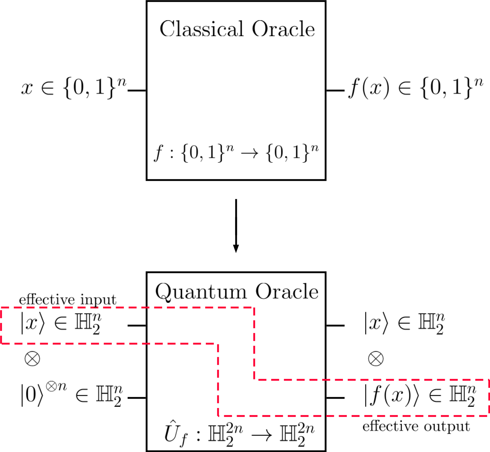
Figure 1: This shows the generalisation of a classical function oracle to a quantum unitary operator oracle, which are maps that perform: $f:\{0,1\}^{n}\rightarrow\{0,1\}^{n}$ and $\hat{U}_{f}:\mathbb{H}_{2}^{2n}\rightarrow\mathbb{H}_{2}^{2n}$ respectively. Note that the qubit lives in the space: $\mathbb{H}_{2}$. The red box in the lower quantum circuit diagram shows the effective input to output of the quantum string as the generalisation of the oracle to a quantum one is reversible.

The quantum version of the oracle acts on a quantum bitstring of length $2n$ instead of $n$. This is a well known technique in quantum generalisations. Since closed quantum evolution is inherently unitary (reversible), we need the oracle to map the initial state, $\ket{x}\otimes\ket{0}^{\otimes n}$, to the final state $\ket{x}\otimes\ket{f(x)}$ in order to make the map reversible. The extra padding of qubits ($\ket{0}^{\otimes n}$ after the effective output) allows the back-tracking of the input given the output, hence the map $\hat{U}_{f}$ is reversible. In summary, Simon’s problem is as follows.

1. $s$ is an $n$ bit string.

2. Blackbox function $f:\{0,1\}^{n}\rightarrow\{0,1\}^{n}$

3. $\exists$ secret string $s\in\{0,1\}^{n}\neq\overbrace{00...000}^{n}$ such that for all inputs $x\in\{0,1\}^{n}$ , $f(x)=f(x\oplus s)$

4. For all inputs $x,y\in\{0,1\}^{n}$, if $x\neq y\oplus s\Rightarrow f(x)\neq f(y)$,

where $\oplus$ is the bitwise modulo 2 addition of two $n$ bitstrings. The game is to find the secret string $s$. Note that the modulo 2 bitwise addition of $s$ to any input $x$ will not change the outcome of the function.

In Simon’s quantum scheme, one has to have access to a $2n$ bitstring long quantum state, $\ket{0}^{\otimes 2n}$ in the computational basis. One applies the gate $\hat{U}_{Simon}=\hat{H}_{a}^{\otimes n}\otimes\mathbb{1}_{2}^{\otimes n}$ to the initial state $\ket{0}^{\otimes 2n}$ before and after the application of the fixed secret string oracle unitary, $\hat{U}_{f}$ as shown in Fig. 2. The matrix $\hat{H}_{a}$ is the 2 by 2 Hadamard matrix and $\mathbb{1}_{2}$ is the 2 by 2 identity matrix. In the basis of the Pauli-$z$ eigenstates $\{\ket{0},\ket{1}\}$, $\hat{H}_{a}=\frac{1}{\sqrt{2}}\begin{bmatrix}1&1\\ 1&-1\\ \end{bmatrix}$. Hence the final state from the quantum circuit is:

$$\ket{final}=\hat{U}_{Simon}\cdot\hat{U}_{f}\cdot\hat{U}_{Simon}\ket{0}^{\otimes 2n}\ \ .$$ (1)

This can be represented using the quantum circuit diagram in Fig. 2 for $n=2$.

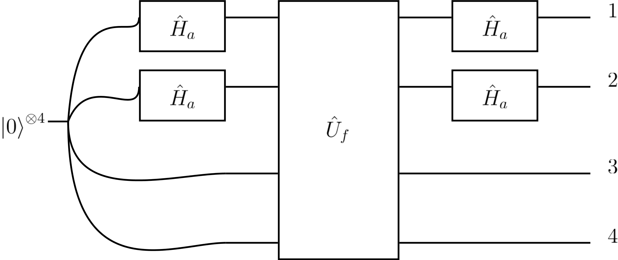
Figure 2: Simon’s quantum circuit for $n=2$. The 2 top qubits are associated with the input to the function and the two lower to the output. Hadamard unitaries create a superposition of inputs. $U_{f}$ enacts the function reversibly, storing the input in the upper two qubits. Hadamards again after $U_{f}$ create further input superposition branching, allowing for interference between terms which originally had different inputs and the same outputs. The number on the right-hand side labels the output port number.

We shall represent the secret string as:

$$s=s_{1}s_{2}...s_{n-1}s_{n}\ \ ,$$ (2)

where $s_{i}\in\{0,1\}$ is the $i^{th}$ bit in the $n$ bit string $s$.

In Simon’s Algorithm, one measures the first register (output port $1$ to $2$ in Fig. 2). This will produce an $n$ bit string, $y$, such that the dot product between $y$ and $s$ in $\mod 2$ is zero, i.e. $y\cdot s=0\pmod{2}$. The algorithm requires repeated inquiries to the oracle, hence obtaining many different $n$ bit strings, $y^{(i)}$, with $i$ indexing the results obtained from each inquiry. The $y$ obtained will be $\{y^{(1)},y^{(2)},y^{(3)},...,y^{(J)}\}$, for $J$ inquiries. Then a classical processing task of Gaussian Elimination in the Galois field $GF(2)$ is carried out to find $s$, represented as follows:

$$\begin{bmatrix}0&0&...&0\\ y_{1}^{(1)}&y_{2}^{(1)}&...&y_{n}^{(1)}\\ \cdot&\cdot&&\\ \cdot&&\cdot&\\ \cdot&&&\cdot\\ y_{1}^{(n-1)}&y_{2}^{(n-1)}&...&y_{n}^{(n-1)}\\ \end{bmatrix}\begin{bmatrix}s_{1}\\ s_{2}\\ \cdot\\ \cdot\\ \cdot\\ s_{n}\\ \end{bmatrix}=\begin{bmatrix}0\\ 0\\ 0\\ 0\\ 0\\ 0\\ \end{bmatrix}\pmod{2}\ \ .$$ (3)

Solving the linear equations in $GF(2)$ is equivalent to only permitting the $s$ vector’s elements to be in $\{0,1\}$, solving the equations in modulo 2.

Since we require that $s$ is not the zero string, only $n-1$ linearly independent equations are needed. The measurement process is probabilistic, meaning sometimes one might not get a set of linearly independent equations to perform Gaussian elimination on, hence one has to inquire the oracle more than $n-1$ times to get a unique solution for $s$, which means $J>n-1$ on average. The Gaussian elimination would have at worst $O(n^{2.3755})$ complexity in time overhead, because the fastest classical algorithm to solve linear equations by Coppersmith and Winograd Coppersmith and Winograd (1990), scales in that manner.

1.2 General Unitary Matrix Parameterisation

We shall train over families of unitaries using techniques from Wan et al. (2017). We shall use a general form of a unitary matrix in terms of Pauli matrices. A general 1 qubit unitary circuit could be written in the forms:

$$\begin{split}\hat{U}^{(1\ qubit)}&=\exp\Bigg{(}i\sum_{j=0}^{3}\alpha_{j}\hat{\sigma}_{j}\Bigg{)},\text{or}\\ \hat{U}^{(1\ qubit)}&=e^{i\alpha_{0}}\Bigg{(}\cos\Omega~{}\mathbb{1}+i\frac{\sin{\Omega}}{\Omega}\sum_{j=1}^{3}\alpha_{j}\hat{\sigma}_{j}\Bigg{)},\end{split}$$ (4)

where $\{\hat{\sigma}_{0},\hat{\sigma}_{1},\hat{\sigma}_{2},\hat{\sigma}_{3}\}$ are the 2 x 2 identity, Pauli-$x$, $y$ and $z$ matrices respectively and $\alpha_{i}\in[0,2\pi)$ and $\Omega=\sqrt{\alpha_{1}^{2}+\alpha_{2}^{2}+\alpha_{3}^{2}}$.

A useful special case with one parameter we will use is $U=\cos(\theta)\hat{\sigma}_{3}+\sin(\theta)\hat{\sigma}_{1}$. A general two qubit unitary could be written in a similar form:

$$\begin{split}\hat{U}^{(2\ qubits)}&=\exp\Bigg{(}i\sum_{j=0}^{3}\sum_{k=0}^{3}\alpha_{j,k}(\hat{\sigma}_{j}\otimes\hat{\sigma}_{k})\Bigg{)}\ \ .\end{split}$$ (5)

2 Methods

2.1 Overall approach

The overall approach is described in Fig. 3. The black-box unitary is given, and the quantum circuit together with the classical post processing needs to learn which states to inject and what type of post-processing to do. There are single-qubit unitaries (or 2 qubit unitaries) with free parameters which get tuned in a systematic manner during the training procedure. There is also a classical post-processing part, which could in principle be a quantum circuit but the number of qubits required would be impractical for simulation/experiments, so it is kept classical.

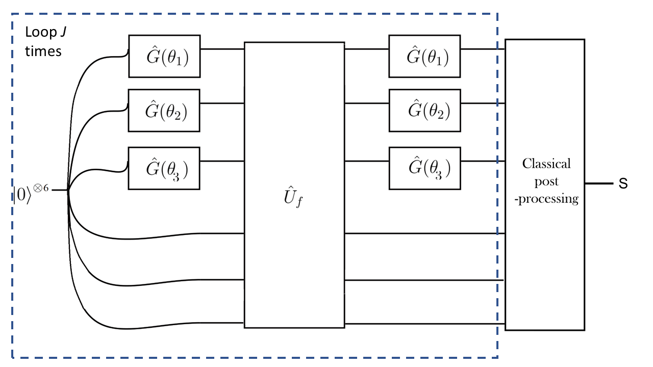
Figure 3: Gradient descent is performed on free parameters $\theta_{1}$, $\theta_{2}$ and $\theta_{3}$, with respect to a single cost function, over all training examples. The quantum part is looped over $J>n-1$ times in line with the technical introduction.

2.2 Number of possible training examples

Lemma 2.1.

The number of 2 to 1 functions of $n$ bitstrings is ${}^{2^{n}}C_{2^{n-1}}$ for a given $s$.

Proof.

There are $2^{n}$ possible $n$ bitstrings. The statement of the lemma is equivalent to saying how many different ways are there to pick $\frac{2^{n}}{2}$ objects from a set of $2^{n}$ objects disregarding ordering.

$\Rightarrow\ ^{2^{n}}C_{2^{n-1}}$ different 2 to 1 functions of $n$ bitstrings. ∎

Lemma 2.2.

For each $n\in\mathbb{Z}$ in Simon’s Problem, there are $(2^{n}-1)\cdot(^{2^{n}}C_{2^{n-1}})$ possible mapping tables.

Proof.

The oracle can have ${}^{2^{n}}C_{2^{n-1}}$ different functions for a given $s$ (using lemma 2.1) and there are $(2^{n}-1)$ different possible $s$ as the problem excludes the zero $n$ bit-string.

$\Rightarrow(2^{n}-1)\cdot(^{2^{n}}C_{2^{n-1}})$ is the number of mapping tables for a specific $n$ in Simon’s Problem. ∎

2.3 Cost function

The cost function, which is the mathematical representation of the aim of the task, is

$$\begin{split}C&=\sum_{\forall s\neq{00...000}}(p_{desired}^{s}-p^{s})^{2},\end{split}$$ (6)

where $p_{desired}^{s}$ is the probability of the output bit string we want it to be and $p^{s}$ is the probability of the measured value. The value of $C$ depends on the free parameters being tuned. This is a supervised learning scenario as the correct $s$ is known and used to evaluate the cost function Nielsen (1991).

2.4 Gradient descent

The quantum circuit is systematically tuned until it reaches a minimum turning point in the cost function. This could be achieved through gradient descent with respect to the $\alpha_{j,k}$ parameters from the unitaries in Eq. 4. Gradient descent is defined as Nielsen (1991):

$$\alpha^{(l)}_{j,k}\rightarrow\alpha^{(l)}_{j,k}-\eta\frac{\partial C}{\partial\alpha^{(l)}_{j,k}},\ \forall j,k\ \ ,$$ (7)

where $\eta\in\mathbb{R}^{+}$ is the step size of the gradient descent and $l$ labels the different unitaries.

2.5 Gradient Descent Assisted Genetic Algorithm Search

Whilst gradient descent works well in many examples, it is a reasonable assumption that optimisation in a high dimensional parameter space may have many local minima. In order to get out of a local minimum de Weck (2010), a Genetic Algorithm is used in the optimisation. This could be done in parallel, which is worthwhile when the computation is done in a supercomputer or using GPUs with a multitude of cores. The gradient assisted genetic algorithm implemented in my system was as follows heuristically:

1. An agent is a random initial guess for the parameters of the unitaries. Start with many agents. This will involve simultaneously initialising many different sets of $\alpha_{j,k}^{(l)}$, with each set being a different agent. The genetic information of each agent is the $\alpha_{j,k}^{(l)}$ parameters.

2. Carry out gradient descent on each agent individually. In this parallelisable procedure, gradient descent is performed for a small number of steps. We shall call this number of steps in gradient descent a generation.

3. After one generation, compare the cost function of each of the agents and find the $\alpha_{j,k}^{(l)}$ of the few agents with the lowest cost. Then repopulate the entire population with the selected few agents with the lowest cost.

4. Apply a small probabilistic random parameter to the $\alpha_{j,k}^{(l)}$ while repopulating the population. This would be analogous to the mutation process in Biology.

5. Repeat the procedure until a minimum is found.

Despite the high computational cost, this method will not guarantee that the final solution will be a global minimum. However, the benefits of this type of search is that the algorithm is now very parallelisable and the mutations added may aid the agents in getting out of a local minima. See Fig. 4 for a pictorial description of the algorithm.

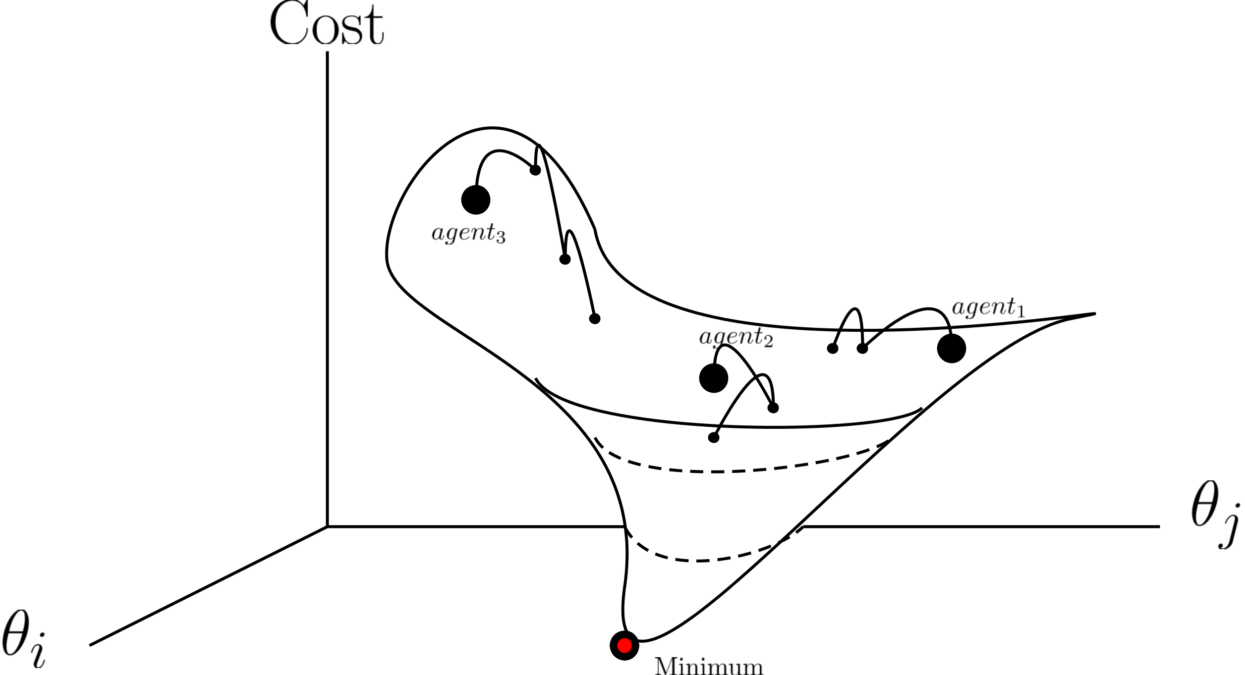
Figure 4: A pictorial representation of how a genetic algorithm works. Many agents are initialised and they are all allowed to propagate to find the minimum.

2.6 Classical post-processing

The classical post-processing takes a set of outputs (the classical bit string $y$’s) and maps them to the corresponding guess for the secret bit-string: $s$. It thus plays an essential role in the algorithm. In Simon’s algorithm this is done by Gaussian elimination modulo 2, as discussed in the technical introduction.

Whilst this part could in principle be enacted with a quantum circuit, as quantum unitary circuits generalise classical computing, that is very costly experimentally and in terms of classical numerical simulation. Our approach here is thus, as depicted in Fig. 3, to include classical post-processing, which takes classical input(s) and then gives the answer: the secret bit string $s$. As Simon’s algorithm and other similar algorithms require several outputs before the classical post-processing, we loop over the quantum part $J$ times to give $J$ classical outputs which are then fed to the classical post-processing.

The classical post-processing amounts to a classical input-output function. This function can be trained as part of the overall training or to make it simpler it can be set by hand to what we want it to be. In the case where only one $s$ was shown to be needed for $n=2$ and $n=3$, the table was set by hand. For $n=2$ we have also tested that the classical part can be trained together with the quantum part rather than set by hand. The training of this part was done by switching one uniformly randomly chosen pair of output bit strings at a time, and accepting the switch only if it decreased the cost function.

3 Results

The main results are summarised as follows.

3.1 Recovering Simon’s Circuit

Results.

A set of restricted unitaries in the form of

$$\hat{G}(\theta_{i})=\begin{bmatrix}\cos(\theta_{i})&\sin(\theta_{i})\\ \sin(\theta_{i})&-\cos(\theta_{i})\end{bmatrix}$$ (8)

could be put in place of the Hadamard matrices in Simon’s original circuit, as shown in Fig. 3, such that gradient descent could be performed on $\theta_{1}$, $\theta_{2}$ and $\theta_{3}$ with respect to the cost function of Eq. 6 to recover Simon’s circuit.

Starting with general single-qubit unitaries yields the same performance as in that restricted single qubit unitary case.

Results.

The same training performed on a set of restricted unitaries in the form of Eq. 4 recovers a circuit with the same performance (same cost function minimum) as Simon’s circuit, but not necessarily the Hadamard gates as in Simon’s circuit.

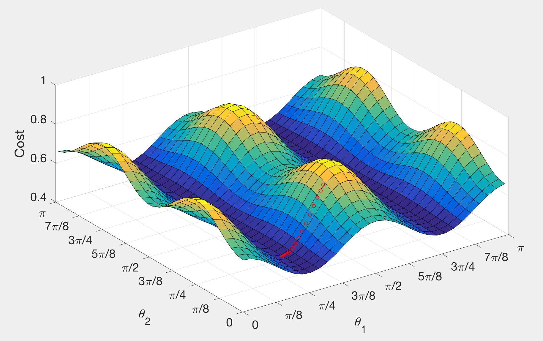
Figure 5: This is the cost landscape sampled under a constant post processing permutation matrix. It can be shown that Simon’s circuit lies in a local minima via the red line which represented the gradient descent path with a starting point close to Simon’s quantum circuit solution parameterised with $\theta_{1}$ and $\theta_{2}$.

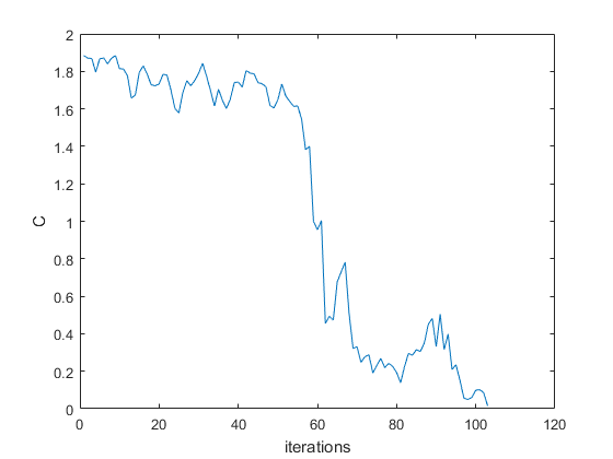
Figure 6: An example of the cost function value as a function of time during training. In this case, $n=3$ and there are 3 free parameters, like those free parameters in Eq. 8.

Fig. 5 illustrates how Simon’s solution $(\theta_{1},\theta_{2})=(\pi/4,\pi/4)$, is a local minimum of the cost function (for n=2). To check if this is truly optimal we did a brute force search over other circuits in this family and confirmed that they never achieve a lower cost value than Simon’s solution. Fig. 6 shows, for $n=3$, parameters staring at a random initial point, can also find the minimum of the cost function, which means can recover Simon’s algorithm. To speed up the classic simulation on computer or high performance computer, we use the parallel computing toolbox in MATLAB, which supports parallel for-loops for running task-parallel algorithms on multiple processors and make the full use of multicore processors on the desktop via workers that run locally.

3.2 Do not need all secret bit strings to train it

We find that we can recover Simon’s algorithm through training with just 1 secret string example for n=2, and 1 secret string for n=3. This is important as there are $2^{n}-1$ such secret strings (the null string is not counted, as it corresponds to a permutation rather than 2-1 function), as discussed earlier. An initial approach, wherein the network would be asked to guess s after just one call to the oracle, required all s’s for the training.

4 Summary and Outlook

We trained a unitary network to find the optimal circuit for solving the task of finding the hidden bit string associated with Simon’s oracle. The result is indeed that the circuit associated with Simon’s algorithm is recovered, such that quantum parallelism is used to probe the oracle unitary. This demonstrates the potential of these techniques for finding algorithms.

We chose Simon’s algorithm as a clean example of the hidden subgroup problem algorithms. It is plausible that the same approach can be used for other problems in that class. A key challenge is to find a task that is technologically useful, such as factoring, but which does not yet have a known quantum algorithm. The current approach combines a human and machine to find the algorithm and making the machine discovery more autonomous may increase the chance of discovering algorithms we have not yet thought of.

Note added: Whilst we were preparing this manuscript, a paper with related ideas, for the case of Grover’s algorithm, appeared on the pre-print server: arXiv:1805.09337, Variationally learning Grover’s Search Algorithm, Morales et al.

Data availability statement

This is a theoretical paper and there is no experimental data available beyond the numerical simulation data described in the paper.

References

- Simon (1997) Daniel R. Simon, “On the power of quantum computation,” SIAM Journal on Computing 26 (5), 1474 – 1483 (1997).
- Shor (1997) Peter W. Shor, “Polynomial-time algorithms for prime factorization and discrete logarithms on a quantum computer,” SIAM J. Comput. 26, 1484–1509 (1997).
- Mermin (2007) N.D. Mermin, Quantum Computer Science: An Introduction (Cambridge University Press, 2007).
- Grigni et al. (2001) Michelangelo Grigni, Leonard Schulman, Monica Vazirani, and Umesh Vazirani, “Quantum mechanical algorithms for the nonabelian hidden subgroup problem,” in Proceedings of the Thirty-third Annual ACM Symposium on Theory of Computing, STOC ’01 (ACM, New York, NY, USA, 2001) pp. 68–74.
- Biamonte et.al. (2016) Biamonte et.al., “Quantum Machine Learning,” (2016), arXiv:1607.08535 .
- Schuld et al. (2014) M. Schuld, I. Sinayskiy, and F. Petruccione, “The quest for a quantum neural network,” Quantum Information Processing 13, 2567–2586 (2014).
- Lloyd et al. (2013) S. Lloyd, M. Mohseni, and P. Rebentrost, “Quantum algorithms for supervised and unsupervised machine learning,” (2013), arXiv:1307.0411 [quant-ph] .
- Lloyd et al. (2014) S. Lloyd, M. Mohseni, and P. Rebentrost, “Quantum principal component analysis,” Nature Physics 10, 631–633 (2014).
- Montanaro (2015) A. Montanaro, “Quantum pattern matching fast on average,” Algorithmica , 1–24 (2015).
- Aaronson (2015) S. Aaronson, “Read the fine print,” Nature Physics 11, 291–293 (2015).
- Garnerone et al. (2012) S. Garnerone, P. Zanardi, and D. A. Lidar, “Adiabatic quantum algorithm for search engine ranking,” Phys. Rev. Lett. 108, 230506 (2012).
- Harrow et al. (2009) A. W. Harrow, A. Hassidim, and S. Lloyd, “Quantum algorithm for linear systems of equations,” Phys. Rev. Lett. 103, 150502 (2009).
- Lloyd et al. (2016) S. Lloyd, S. Garnerone, and P. Zanardi, “Quantum algorithms for topological and geometric analysis of big data,” Nature Communications 7, 10138 (2016).
- Rebentrost et al. (2014) P. Rebentrost, M. Mohseni, and S. Lloyd, “Quantum support vector machine for big data classification,” Phys. Rev. Lett. 113, 130503 (2014).
- Wiebe et al. (2012) N. Wiebe, D. Braun, and S. Lloyd, “Quantum algorithm for data fitting,” Phys. Rev. Lett. 109, 050505 (2012).
- Adcock et al. (2015) J. Adcock, E. Allen, M. Day, S. Frick, J. Hinchliff, M. Johnson, S. Morley-Short, S. Pallister, A. Price, and S. Stanisic, “Advances in quantum machine learning,” (2015), arXiv:1512.02900 [quant-ph] .
- Heim et al. (2015) B. Heim, T. F. Rønnow, S. V. Isakov, and M. Troyer, “Quantum versus classical annealing of Ising spin glasses,” Science 348, 215–217 (2015).
- Gross et al. (2010) D. Gross, Y.K. Liu, S. T. Flammia, S. Becker, and J. Eisert, “Quantum state tomography via compressed sensing,” Phys. Rev. Lett. 105, 150401 (2010).
- Dunjko et al. (2016) V. Dunjko, J. M. Taylor, and H. J. Briegel, “Quantum-enhanced machine learning,” Phys. Rev. Lett. 117, 130501 (2016).
- Wittek (2014) P. Wittek, ed., Quantum Machine Learning (Academic Press, Boston, 2014).
- Bisio et al. (2010) A. Bisio, G. Chiribella, G. M. D’Ariano, S. Facchini, and P. Perinotti, “Optimal quantum learning of a unitary transformation,” Phys. Rev. A 81, 032324 (2010).
- Sasaki and Carlini (2002) M. Sasaki and A. Carlini, “Quantum learning and universal quantum matching machine,” Phys. Rev. A 66, 022303 (2002).
- Bang et al. (2008) J. Bang, J. Lim, M. S. Kim, and J. Lee, “Quantum Learning Machine,” ArXiv e-prints (2008), arXiv:0803.2976 [quant-ph] .
- Sentís et al. (2015) G. Sentís, M. GuŢă, and G. Adesso, “Quantum learning of coherent states,” EPJ Quantum Technology 2, 17 (2015).
- Banchi et al. (2016) L. Banchi, N. Pancotti, and S. Bose, “Quantum gate learning in qubit networks: Toffoli gate without time-dependent control,” Npj Quantum Information 2, 16019 EP – (2016).
- Palittapongarnpim et al. (2016) P. Palittapongarnpim, P. Wittek, E. Zahedinejad, S Vedaie, and B. C. Sanders, “Learning in quantum control: high-dimensional global optimization for noisy quantum dynamics,” (2016).
- Wan et al. (2017) K. H. Wan, O. Dahlsten, H. Kristjánsson, R. Gardner, and M. S. Kim, “Quantum generalisation of feedforward neural networks,” npj Quantum Information 3, 36 (2017).
- Vazirani (2004) Umesh V. Vazirani, “Simon’s algorithm,” (2004), unpublished.
- Coppersmith and Winograd (1990) Don Coppersmith and Shmuel Winograd, “Matrix multiplication via arithmetic progressions,” Journal of Symbolic Computation 9 (3), 251 (1990).
- Nielsen (1991) M. A. Nielsen, Neural Networks and Deep Learning (Determination Press, online book, 1991).
- de Weck (2010) Olivier de Weck, “A basic introduction to genetic algorithms,” (2010), online notes, unpublished.
- Wan (2017) Kwok Ho Wan, “The power of quantum computation-a new perspective, Imperial College London,” (2017), B.Sc. Thesis.