Assisted exchange models in one dimension

Abstract

We introduce an assisted exchange model (AEM)on a one dimensional periodic lattice with $K+1$ different species of hard core particles, where the exchange rate depends on the pair of particles which undergo exchange and their immediate left neighbor. We show that this stochastic process has a pair factorized steady state for a broad class of exchange dynamics. We calculate exactly the particle current and spatial correlations $(K+1)$-species AEM using a transfer matrix formalism. Interestingly the current in AEM exhibits density dependent current reversal and negative differential mobility- both of which have been discussed elaborately by using a two species exchange model which resembles the partially asymmetric conserved lattice gas model in one dimension. Moreover, multi-species version of AEM exhibits additional features like multiple points of current reversal, and unusual response of particle current.

I Introduction

Non-equilibrium phenomena book1 are very common in nature and occur whenever there is a net unbalanced flux of some physical observable like mass, charge etc. along some particular direction- this net flow of physical quantities, commonly termed as current is one of the most intriguing feature that characterizes non-equilibrium systems(NES) in contrast to their equilibrium counterparts which are identified as zero-current states. While the stationary states of equilibrium systems are quantified by the very well known Gibbs measure or Boltzmann distribution, the steady state measure of non-equilibrium systems has no unique identity and has always been a question of interest in the quest of NES. In this context, finding current or net flux in these non-equilibrium steady states and studying several features of the current in order to understand and characterize non-equilibrium systems has become one of the primary interests. For example, the exact large deviation function of the time averaged current resembling to the pressure of an ideal Bose or Fermi gas is obtained in cur_press , anomalous behavior of cumulants of current near phase transition is shown in cfluc_phse_tran , universal behavior of current independent of the dimension in symmetric exclusion process connected to reservoirs and its possible generalization to other diffusive systems is discussed in cur_universal . Also, interesting features like reversal of direction of current with respect to density crev_azrp and negative differential mobility ndm_1 ; ndm_2 ; ndm_3 ; ndm_4 and absolute negative mobility anm_1 ; anm_2 ; anm_3 in interacting particle systems has caused much attention now a days.

Driven diffusive systems(DDS) has been central to the study of non-equilibrium systems in the recent years as they exhibit several interesting features like phase transitions even in one dimension book2 and have a wide variety of applications book3 in different branches of physics. A typical example of DDS that has been widely studied in context of both non-equilibrium phase transitions asep_1 and current asep_2 ; asep_3 in NES, is the asymmetric exclusion process book4 . In particular, asymmetric exclusion process has been used to study extensively current, current fluctuations and its higher order cumulants in asep_4 ; asep_5 ; asep_6 and significant comparison of large deviation functions of current with the notion of equilibrium free energy asep_7 has been made. Also, the asymmetric exclusion process has also been generalized to multi-species asep_8 , restricted exclusion process asep_9 and others in different contexts.

In this article we introduce assisted exchange models on a one dimensional periodic lattice where each site can occupy at most one particle of type $k=0,1,\dots K.$ A particle at any site can exchange their position with one of their nearest neighbors with a rate that depends on both, the type of particle pair which are exchanged, and the type of particle present at the left most neighbour of the exchanging-pair. We primarily address two questions about the ($K+1$)- species assisted exchange models (AEM). The first one is to find the exact steady state measure of this non-equilibrium system- in particular we derive the condition on exchange rates that give rise to pair factorized steady states (PFSS). We argue that for any finite $K,$ a pair factorized steady state can not give rise to phase separation transition; in other words the systems in this case remains in a mixed phase exhibiting nontrivial spatial correlations. We also aim at obtaining the exact steady state current of each particle species. It turns out that AEM exhibits density dependent current reversal and negative differential mobility of particle current, which have been subjects of interest in recent times crev_azrp ; ndm_4 .

Multi-species models with simple exchange dynamics, where exchange of different type of particle pairs occur with different rates, have been introduced earlier Isaev . It turns out that steady state of these models can not be written in pair-factorized form, but there can be a matrix product steady state with matrices satisfying a diffusion algebra. Some explicit examples of these models with $K=1,2$ have been discussed in Refs. ZRP_rev ; Isaev . In fact, asymmetric or symmetric exclusion process ($K=1$) book4 belong to these class of models with $K=1.$ Some other examples, with $K=2$ are two species exclusion models ZRP_rev , ABC model ABC1 ; ABC2 and extended AHR model AHR ; some of these models, like ABC model, exhibits phase separation transition in one dimension.

The article is organized as follows. In section II we introduce the model and derive a condition on rate functions that give rise to a pair-factorized steady states for a broad class of dynamics. Here we introduce a transfer matrix formulation to calculate the steady state current and spatial correlations. In section III, we introduce a class of exactly solvable assisted exchange model (AEM) for which the spatial correlations, particle current and density-fugacity relations can be calculated exactly for any arbitrary $K.$ Some specific examples with $K=1$ and $K=2$ are discussed in section IV and V respectively. We find that the exchange models exhibits several interesting phenomena: reversal of current as particle density is changed, negative differential mobility, double extrema in current voltage relation etc. Lastly, we conclude in section VI with some discussions.

II Model

Consider a system of $(K+1)$species of particles on a one dimensional periodic lattice with $L$ sites represented by $i=1,2,\dots,L.$ Each site $i$ can be occupied by at most one particle of type $k=0,1,\dots,K$; accordingly the site variable $s_{i}$ takes an non-negative integer value smaller than $(K+1).$ The dynamics of the model is given by

$$XIJ\mathop{\leftrightharpoons}_{w(XJI)}^{w(XIJ)}XJI,$$ (1)

where $w(XIJ)>0$ are the exchange rates, which need not have a functional form as the arguments of $w(.)$ only specify the type of particles. Although $k$ being an integer provide a notion of ordering, the ordering here does not carry any physical meaning; in other words the type particle could have been represented by any other symbols, not necessarily by an integer, like $k=a,b,\dots.$ Clearly this dynamics (1) conserves the particle number $N_{k}$ of each kind - the model has $K$ conservation laws along with the trivial one $\sum_{k=0}^{K}N_{k}=L.$

In some examples we discuss here, $k=0$ are considered as vacant sites; in that case there are only $K$-species of particles of type $k=1,2,\dots,K;$ the exchange of a particle with $0$ present in the left (or right) neighbor will then represent hopping of that particle to left or right - the density conservation of each species $\rho_{k}=\frac{N_{k}}{L}$, where $N_{k}$ is the number of particles of type $k$, remains unaltered.

II.1 Steady state

The Master Equation describing the time evolution of the probabilities of different configurations following the dynamics (1) is as follows

$$\frac{d}{dt}P(\{s_{i}\}) = \sum_{i=1}^{L}u(s_{i-1},s_{i+1},s_{i})P(\dots s_{i-1},s_{i+1},s_{i},s_{i+2}\dots)$$ (2)

$$- \sum_{i=1}^{L}u(s_{i-1},s_{i},s_{i+1})P(\dots s_{i-1},s_{i},s_{i+1},s_{i+2}\dots)$$ (3)

Our first goal is to find the steady state by setting the left hand side of Eq.(3) equal to zero. It seems to be quite complex to obtain the steady state for the general dynamics (1) . Instead we look for class of rates for which we can have a pair factorized steady state (PFSS) for this assisted hopping and exchange model. In case of PFSS (which by construction is a spatially correlated state in contrast to factorized steady states that may be simpler to achieve but do not contain spatial correlations among its constituents), the steady state weight of any possible configuration is expressed as a product of pairs of a function of successive neighbors on the lattice. Explicitly, the steady state weight of any configuration $\{s_{i}\}$ is given by

$$P(\{s_{i}\})\sim\prod_{i=1}^{L}g(s_{i},s_{i+1})\prod_{k=1}^{K}\delta\left(\sum_{i=1}^{L}\delta_{s_{i},k}-N_{k}\right)$$ (4)

The right hand side of (3) contains the sum of numerous in-flux and out-flux terms, which must equal to zero in the steady state; this cancellation can happen in several ways. To achieve the PFSS described in (4), it is sufficient to follow the condition

$$u(s_{i-1},s_{i+1},s_{i})\frac{g(s_{i-1},s_{i+1})g(s_{i+1},s_{i})g(s_{i},s_{i+2})}{g(s_{i-1},s_{i})g(s_{i},s_{i+1})g(s_{i+1},s_{i+2})}-u(s_{i-1},s_{i},s_{i+1})$$ (5)

$$~{}~{}~{}~{}~{}=h(s_{i-1},s_{i},s_{i+1})-h(s_{i},s_{i+1},s_{i+2})$$ (6)

where the function $h(.)$ are yet to be determined suitably. Note the right hand side of the condition Eq. (6), when summed over all lattice sites gives zero and ensures stationary, $\frac{d}{dt}P(\{s_{i}\})=0.$ It is now straight forward to check that the follwing rate functions satisfy Eq. (6)

$$u(s_{i-1},s_{i},s_{i+1}) = \frac{g(s_{i-1},s_{i+1})}{g(s_{i-1},s_{i})g(s_{i},s_{i+1})}~{}~{}~{}~{}\mathrm{if}~{}~{}~{}s_{i}\neq s_{i+1}$$ (7)

$$= 0~{}~{}~{}~{}\mathrm{if}~{}~{}~{}s_{i}=s_{i+1}$$ (8)

with

$$h(s_{i-1},s_{i},s_{i+1}) = -u(s_{i-1},s_{i},s_{i+1})~{}~{}~{}~{}\mathrm{if}~{}~{}~{}s_{i}\neq s_{i+1}$$ (9)

$$= 0~{}~{}~{}~{}\mathrm{if}~{}~{}~{}s_{i}=s_{i+1}.$$ (10)

II.2 Transfer matrix formulation

The next task would be to calculate the partition function and the observables of the $(K+1)$-species exchange model, which is,

$$Q(\{N_{k}\}) = \sum_{\{s_{i}\}}\prod_{i}g(s_{i},s_{i+1})\prod_{k}\delta\left(\sum_{i}\delta_{s_{i},k}-N_{k}\right).$$ (11)

The $\delta$-functions ensure that the particle numbers ($N_{k}$-s) are conserved. We now work in the grand canonical ensemble(GCE) and associate fugacities $\{z_{k}\},$ one for each species, which will control the particle densities $\{\rho_{k}\}.$ Also we set $z_{0}=1,$ without loss of generality. Hence the partition function in the GCE is

$$Z(\{z_{k}\}) = \sum_{\{N_{k}\}}^{\infty}Q(\{N_{k}\})\prod_{k}(z_{k})^{N_{k}}$$ (12)

$$= \sum_{\{s_{i}\}}\prod_{i}z_{s_{i}}g(s_{i},s_{i+1})=\mathrm{Tr}[T^{L}]$$ (13)

where $T$ is a $(K+1)$ dimensional square matrix

$$T=\sum_{k^{\prime},k=0}^{K}g(k^{\prime},k)z_{k}|k^{\prime}\rangle\langle k|$$ (14)

which is formally known as the transfer matrix. Here $\{|k\rangle\}$ with $k=0,1,\dots,K$ are the standard basis vectors in $(K+1)$-dimension. The transfer matrix $T$ can also be written as

$$T=\sum_{k=0}^{K}z_{k}D_{k}~{}~{}{\rm with}~{}~{}D_{k}=\sum_{k^{\prime}=0}^{K}g(k^{\prime},k)|k^{\prime}\rangle\langle k|$$ (15)

where the matrix $D_{k}$ represents a particle of the species $k.$ With these set of matrices $\{D_{k}\}$ we write the steady state weights of the system in matrix product form

$$P(\left\{s_{i}\right\})\sim\prod_{i}g(s_{i},s_{i+1})=\mathrm{Tr}[\prod_{i}D_{s_{i}}]$$ (16)

In matrix product form, the correspondence of particles by a representing matrix, helps in calculating expectation values of several observables, which is discussed below.

With Eq.(15) in hand, we can proceed to calculate different observables analytically. Let us start with density $\rho_{k}$ of the particles of species $k.$

$$\rho_{k}=\langle k\rangle=\frac{\mathrm{Tr}[z_{k}D_{k}T^{L-1}]}{\mathrm{Tr}[T^{L}]}=\frac{\langle k|T^{L}|k\rangle}{\mathrm{Tr}[T^{L}]},$$ (17)

Let the eigenvalues of $T$ are $\lambda>\lambda_{1}\geq\lambda_{2}\dots\geq\lambda_{K}$ with corresponding right and left eigenvectors (normalized) $\{|\psi\rangle,|\psi_{1}\rangle,|\psi_{2}\rangle\dots|\psi_{K}\rangle\}$ and $\{\langle\phi|,\langle\phi_{1}|,\langle\phi_{2}|\dots\langle\phi_{K}|\rangle\}$ respectively. Since $T$ is a positive matrix (as $g(i,j)>0),$ the largest eigenvalue $\lambda$ is non-degenerate and the corresponding eigenvector $|\psi\rangle$ can be chosen positive. Thus,

$$T^{n}=\lambda^{n}|\psi\rangle\langle\phi|+\sum_{k=1}^{K}\lambda_{k}^{n}|\psi_{k}\rangle\langle\phi_{k}|$$ (18)

Using this in Eq. (17) we calculate the density of each species in the thermodynamic limit $L\rightarrow\infty$ ( i.e. $\lambda^{L}\gg\lambda_{k}^{L}~{}\forall 1\leq k\leq K$),

$$\rho_{k}=\langle k|\psi\rangle\langle\phi|k\rangle.$$ (19)

In a similar way one can calculate expectation values, that species $k$ is a right neighbor of $m$ in steady state,

$$\langle mk\rangle = \frac{\mathrm{Tr}[z_{m}z_{k}D_{m}D_{k}T^{L-2}]}{\mathrm{Tr}[T^{L}]}$$ (20)

$$= \frac{z_{k}g(m,k)}{\lambda}\langle k|\psi\rangle\langle\phi|m\rangle,$$ (21)

where in the last step we have used the thermodynamic limit. In a similar manner, one can obtain the two-point spatial correlation functions between any two species of particles (say $k$ and $k^{\prime}$) at a distance $r$,

$$C_{k,k^{\prime}}(r) = \frac{\mathrm{Tr}[z_{k}D_{k}T^{r-1}z_{k^{\prime}}D_{k^{\prime}}T^{L-r-1}]}{\mathrm{Tr}[T^{L}]}-\rho_{k}\rho_{k^{\prime}}$$ (22)

$$= \frac{\langle k|T^{r}|k^{\prime}\rangle\langle k^{\prime}|T^{L-r}|k\rangle}{\mathrm{Tr}[T^{L}]}-\rho_{k}\rho_{k^{\prime}}$$ (23)

$$= \langle k^{\prime}|\psi\rangle\langle\phi|k\rangle\sum_{m=1}^{K}\langle k|\psi_{m}\rangle\langle\phi_{m}|k^{\prime}\rangle\left(\frac{\lambda_{m}}{\lambda}\right)^{r}.$$ (24)

Here, to obtain the last step, we used Eq. (19) and taken the thermodynamic limit. For large $r,$ the dominant contribution to the correlation function comes from the first term $m=1$ (in the sum), i.e. $C_{k,k^{\prime}}(r)\sim~{}(\frac{\lambda_{1}}{\lambda})^{r}=e^{-r/\xi}$ where the correlation length $\xi=(\ln\frac{\lambda_{1}}{\lambda})^{-1}.$

From the study of correlation functions it is clear that a pair factorized steady state can not give rise to diverging correlation length if the number of species are finite. For $(K+1)$ species model, one gets $(K+1)-$ dimensional transfer matrix with elements $\langle m|T|n\rangle=z^{m}g(m,n)>0;$ the largest eigenvalue $\lambda$ then remains non-degenerate following Perron-Frobenius theorem. Thus, the correlation length $\xi=(\ln\frac{\lambda_{1}}{\lambda})^{-1}$ is finite and possibility of phase transition is ruled out in $(K+1)$ component systems with PFSS. To get out of this situation, one may think of setting some matrix elements to zero so that the transfer matrix become reducible and then, Perron-Frobenius theorem (non-degenerate largest eigenvalue) does not apply. However, it is easy to check that a reducible form of $g(m,n)$ force the steady state weight of all configurations to be zero.

There are numerous examples of exchange models which exhibit phase transition; like extended KLS models with ferro EKLS or anti-ferromagnetic AF interactions, ABC models in an interval ABC2 or a ring ABC1 . However, the steady state of these models are not pair factorized. In some models, the steady state can be written in matrix product form MPA with matrices having dimensions larger than the number of components $(K+1)$, then the matrix elements of corresponding transfer matrix can not be treated as the weight factors, as in PFSS. In this case one can have a reducible transfer matrix which does not restrict the phase space even though a block of matrix elements are zero.

The assisted exchange models, with factorized steady state, does not give rise to phase separation transitions in general, but they exhibit interesting steady-state current behavior which will be discussed in the next section.

II.3 Average current of particles

The average current is an entity of interest since the non-equilibrium phenomena are characterized by a net flow or current in the system comparing to their equilibrium counterparts which are dictated by zero average current. In this section we will focus on calculating exactly the average particle current in the pair factorized steady states of $(K+1)$species assisted exchange models. In particular, the average current for the species $k$ would be

$$\langle J_{k}\rangle=\sum_{k^{\prime}\neq k}^{K}\sum_{m=0}^{K}u(m,k,k^{\prime})\langle mkk^{\prime}\rangle-u(m,k^{\prime},k)\langle mk^{\prime}k\rangle$$ (25)

Using the matrix representations in Eq. (15), it is quite straightforward to obtain

$$\langle mkk^{\prime}\rangle = \frac{z_{k}z_{k^{\prime}}}{\lambda^{2}}g(m,k)g(k,k^{\prime})\langle k^{\prime}|\psi\rangle\langle\phi|m\rangle$$ (26)

$$= \frac{\langle mk\rangle\langle kk^{\prime}\rangle}{\rho_{k}}$$ (27)

Then, for the exchange dynamics (8), the current of species $k$ is

$$\langle J_{k}\rangle = \frac{1}{\lambda^{2}}\sum_{k^{\prime}\neq k}^{K}\sum_{m=0}^{K}z_{k}z_{k^{\prime}}\langle\phi|m\rangle\left(g(m,k^{\prime})\langle k^{\prime}|\psi\rangle-g(m,k)\langle k|\psi\rangle\right)$$ (28)

$$= \frac{1}{\lambda}\sum_{k^{\prime}\neq k}^{K}\sum_{m=0}^{K}\left(z_{k}\langle mk^{\prime}\rangle-z_{k^{\prime}}\langle mk\rangle\right)$$ (29)

To proceed further we need to be more specific about the dynamics. In the following section we choose a specific form of weight function $g(m,n)$ for which the steady state results for current and other observables can be obtained exactly for any any arbitrary $K.$

III Exact results for a class of AEM

In this section we choose a specific form of weight function $g(m,n)$ for which the steady state calculations of current can be done explicitly for any arbitrary $K.$ Let us consider a weight function

$$g(m,n) = \frac{g(m,0)g(0,n)}{\gamma g(0,0)}~{}~{}~{}m,n>0,$$ (30)

where $g(m,0)$ and $g(0,n)$ are $2K+1$ independent parameters; once these parameters are fixed, the rest of the elements of $g(m,n)$ can be calculated using Eq. (30). In the following, for convenience, we set a short-hand notation

$$v_{m}=g(m,0)g(0,m).$$ (31)

It is easy to check that the transfer matrix $T,$ with elements $\langle m|T|n\rangle=z_{m}g(m,n)$ along with Eq. (30), has the following properties,

$$I. ~{}\mathrm{Tr}[T]=\sum_{k=0}^{K}z_{k}g(k,k)\equiv 2\tau$$ (32)

$$II. ~{}\mathrm{Det}[T]=0$$ (33)

$$III. ~{}{\rm Eigenvalues:}\left\{\lambda_{\pm}=\tau\pm\sqrt{\tau^{2}-\delta},0,0,\dots\right\},~{}~{}~{}~{}\delta\equiv(\gamma^{-1}-1)\prod_{k=1}^{K}z_{k}g(k,k)$$ (34)

Let $|\psi\rangle,$ and $\langle\phi|$ be the left and right eigenvectors (normalized), corresponding to the largest eigenvalue $\lambda\equiv\lambda_{+}$ with elements, $\langle m|\psi\rangle,$ and $\langle\phi|m\rangle$ with $m=0,1,2,\dots K.$ For $m>0$ we have,

$$\langle m|\psi\rangle = \eta~{}g(m,0)\langle 0|\psi\rangle;~{}\langle\phi|m\rangle=\eta~{}z_{m}g(0,m)\langle\phi|0\rangle;~{}~{}{\rm with}~{}~{}\eta=\frac{\lambda+(\gamma-1)g(0,0)}{\gamma g(0,0)\lambda}.$$ (35)

For $m=0,$ one can determine $\langle 0|\psi\rangle$ and $\langle\phi|0\rangle$ from the normalization condition $\langle\phi|\psi\rangle=1,$

$$\langle\phi|0\rangle\langle 0|\psi\rangle=\left(1+2\eta^{2}\tau-\eta^{2}g(0,0)\right)^{-1}$$ (36)

Using these properties of $T$ it is straight forward to calculate the observables - we state the results in the following. Let us use the grand canonical ensemble and remind ourselves that, without loss of generality, we can set the fugacity $z_{0}=1.$ The particle densities are then

$$\rho_{m}=\frac{\gamma z_{m}v_{m}g^{2}(1,1)}{2\alpha^{\prime}\alpha}\left[\alpha^{\prime}+\alpha-v_{1}^{2}\right]$$ (37)

where,

$$\alpha^{\prime}=\sqrt{(\alpha+v_{1}^{2})^{2}+4(\gamma-1)\alpha v_{1}^{2}}$$ (38)

$${\rm and}~{}\alpha=\gamma g^{2}(1,1)\sum_{k=1}^{K}z_{k}v_{k}.$$ (39)

Similarly, the correlation function is

$$C_{m,m^{\prime}}(r)=\frac{\gamma z_{m^{\prime}}g(m,0)g(0,m^{\prime})g^{2}(1,1)}{2\alpha^{\prime}\alpha}\left[\alpha^{\prime}-\alpha+v_{1}^{2}\right]\left(\frac{\lambda_{-}}{\lambda}\right)^{r}$$

This being stated, we now proceed to obtain the particle current given by (29). From now onwards, we will be concerned with the average current of the species $k=0.$ As we have already mentioned that $k=0$ can be considered as vacant sites and $k>0$ as the $K$-particle species; the particles $k=1,2,\dots,K$ exchange with each other whereas the exchange of any species $k$ with $0$ will now represent diffusion, i.e., hopping of that species to right or left vacant neighbour. Clearly in this case the total current including that of $0$ or vacant sites will be $\langle J\rangle+\langle J_{0}\rangle=0$ where $\langle J\rangle$ is the total particle current of $K$-species of particles $k=1,2,\dots,K.$ Then, $\langle J\rangle=-\langle J_{0}\rangle.$ Current $\langle J_{0}\rangle$ can be calculated from Eq. (29), which gives the total particle current

$$\langle J\rangle=\frac{1}{\lambda^{2}}\left[(\rho_{0}g(0,0)+\sqrt{\rho_{0}}s_{k})\sum_{i=1}^{k}z_{i}-(\sqrt{\rho_{0}}+\frac{1}{\gamma g(0,0)}s_{k})s_{k}\right]$$ (40)

$$\mathrm{where}~{}~{}~{}s_{k}=\sum_{i=1}^{k}\sqrt{\rho_{i}z_{i}v_{i}}.$$

Inverting the density fugacity relations, we arrive at the following equation

$$z_{i}=\frac{\rho_{i}}{v_{i}}\frac{(v_{1})^{K-1}}{2g^{2}(1,1)\rho_{0}(1-\rho_{0})^{2}}[~{}~{}v_{1}(1-2\rho_{0})^{2}+2g(0,0)g(1,1)\rho_{0}(1-\rho_{0})$$ (41)

$$+(1-2\rho_{0})\sqrt{v_{1}(v_{1}(1-2\rho_{0})^{2}+4g(0,0)g(1,1)\rho_{0}(1-\rho_{0}))}~{}~{}],$$ (42)

(43)

that expresses the fugacities $z_{i}(i=1,2,\dots,k)$ in terms of the densities $\rho_{i}$ so that $z_{i}$ can be replaced in Eq. (40). Note the difference between the expressions of the average particle current $\langle J\rangle$ in (40) compare to (29)-in case of (40), it became possible to write down the current only in terms of the input parameters like the densities and hop rates(after replacing $z_{i}$s using (43)) -which was not that straightforward for (29).

Now, as we have obtained the exact average current for the $K-$species assisted exchange model studied in this article, our next move would be to investigate possible interesting properties of the current. First we consider next a simple case with $K=1$ i.e. a single species of particles undergoing assisted hopping on a $1-$D periodic lattice and we will discuss phenomenas like density dependent current reversal, negative differential mobility of particles in detail for this simple example.

IV Assisted exchange model with $K=1$

Consider a $1-$D periodic lattice with $L$ sites $i=1,2,\dots,L$ where each site $i$ can be occupied by at most one particle(i.e.the particles are hard core), each represented by $1$ or it can be vacant, represented by $0$. A particle from a randomly chosen site $i$ can move to its right neighbor(if vacant) $(i+1)$ with a rate that depends on the left neighbor $(i-1)$ of the departure site. Whereas, the particle from $i$ can also move to its left neighbor(if vacant) $(i-1)$ with a rate that depends on the left neighbor $(i-2)$ of the arrival site $(i-1)$. More precisely, in a nutshell, the motion of the particles are assisted by their neighbors- isolated particles and crowded particles(particles with occupied neighbors) hop in different manner. The dynamics is represented as

$$010\mathop{\rightleftharpoons}_{q}^{p}001~{}~{}~{}~{}~{}~{}~{}~{}~{}~{}110\mathop{\rightleftharpoons}_{\gamma_{2}q}^{\gamma_{1}p}101$$ (44)

For this dynamics we have pair factorized steady state, following (8) only if $\gamma_{1}=\frac{1}{\gamma_{2}}\equiv\gamma$; the pair-weight functions are then

$$g(0,0)=\frac{1}{q};~{}g(1,0)g(0,1)=v_{1}=\frac{1}{pq};g(1,1)=\frac{1}{\gamma p}$$ (45)

and the corresponding dynamics,

$$010\mathop{\rightleftharpoons}_{q}^{p}001~{}~{}~{}~{}~{}~{}~{}~{}~{}~{}110\mathop{\rightleftharpoons}_{q\gamma^{-1}}^{\gamma p}101$$ (46)

has three parameters $p,q$ and $\gamma.$ It is easy to show that the particle current for this single species assisted exchange model ultimately becomes

$$\langle J\rangle=p(\langle 010\rangle+\gamma\langle 110\rangle)-q(\langle 001\rangle+\frac{1}{\gamma}\langle 101\rangle)=\frac{1}{\lambda^{2}}\left[z_{1}(\frac{\rho_{0}}{q}-\frac{\rho_{1}}{\gamma p})+(z_{1}-1)\sqrt{\frac{\rho_{0}\rho_{1}z_{1}}{pq}}\right]$$ (47)

$$\mathrm{where}~{}~{}~{}\lambda=\frac{1}{2}\left(\frac{1}{q}+\frac{z_{1}}{\gamma p}+\sqrt{(\frac{1}{q}-\frac{z_{1}}{\gamma p})^{2}+4\frac{z_{1}}{pq}}\right).$$

In the above equation, we have calculated the current in the grand canonical ensemble by associating a fugacity $z_{1}$ to the particles. In order to express the average current $\langle J\rangle$ in terms of particle or vacancy densities, one can replace $z_{1}$ in (47) by inverting the density-fugacity relation as follows

$$z_{1} = \frac{\gamma p}{q}+\frac{(1-2\rho_{0})\gamma^{2}p^{2}}{2\rho_{0}(1-\rho_{0})}\left[\frac{1}{pq}(1-2\rho_{0})+\sqrt{\frac{1}{pq}(\frac{(1-2\rho_{0})^{2}}{pq}+4\frac{\rho_{0}(1-\rho_{0})}{\gamma pq})}\right].~{}~{}~{}~{}~{}$$ (48)

Now we would like to discuss two interesting features viz. density dependent current reversal and negative differential mobility of particles emerging from the expression of particle current in Eq. (47) that resulted from the stochastic process (44) along with (45).

IV.1 Current reversal in AEM with $K=1$

Let us discuss a more specific example with, $q=\frac{1}{p}$ and $\gamma=\frac{1}{p^{2}};$ the dynamics is then,

$$010\mathop{\rightleftharpoons}_{\frac{1}{p}}^{p}001~{}~{}~{}~{}~{}~{}~{}~{}~{}~{}110\mathop{\rightleftharpoons}_{p}^{\frac{1}{p}}101~{}~{}.$$ (49)

Now comparing the rates in Eq. (49) with that in (44) and further using Eq. (45), we conclude that the dynamics in (49) indeed gives rise to a pair factorized steady state with the pair weight factors obtained as $g(1,0)=g(0,1)=1$ and $g(0,0)=g(1,1)=p$. Correspondingly, the particle current from Eq. (47) will be

$$\langle J\rangle=\frac{1}{\lambda^{2}}\left[z_{1}p(\rho_{0}-\rho_{1})+(z_{1}-1)\sqrt{\rho_{0}\rho_{1}z_{1}}\right],$$ (50)

where $\lambda=\frac{1}{2}(p(1+z_{1})+\sqrt{p^{2}(1-z_{1})^{2}+4z1})$. But the above expression can be further simplified if we use the fact $\rho_{0}=1-\rho_{1}$ and also note that the fugacity in Eq. (48) subsequently becomes

$$z_{1}=1+\frac{(2\rho_{1}-1)}{2p^{2}\rho_{1}(1-\rho_{1})}\left[2\rho_{1}-1+\sqrt{(2\rho_{1}-1)^{2}+4p^{2}\rho_{1}(1-\rho_{1})}\right].$$ (51)

Then the current takes the functional form as follows

$$\langle J\rangle=\frac{(2\rho_{1}-1)}{\lambda^{2}}\left[pz_{1}+\frac{\sqrt{\rho_{1}(1-\rho_{1})z_{1}}}{2p^{2}\rho_{1}(1-\rho_{1})}\left(2\rho_{1}-1+\sqrt{(2\rho_{1}-1)^{2}+4p^{2}\rho_{1}(1-\rho_{1})}\right)\right]~{}~{}~{}~{}~{}$$ (52)

Note that in principle, we should have replaced $z_{1}$ all the way through Eq. (52) by using (51), but keeping $z_{1}$ intact in some places other than the required does not harm our purpose of showing density dependent current reversal from (52). More precisely, to observe current reversal by changing particle density for a fixed dynamics, we have to have the current $\langle J\rangle$ in Eq. (52) equal to zero for some non-zero value of the particle density $\rho_{1}=\rho^{\ast}_{1}.$ As a careful observation ensures the fact that the entities involving $z_{1}$ in the expression of $\langle J\rangle$ in Eq. (52) are always greater than zero, so the only possibility to obtain density dependent current reversal i.e. $\langle J\rangle=0$ in (52) for the fixed dynamics (49) is to set $\rho^{\ast}_{1}=\frac{1}{2}.$

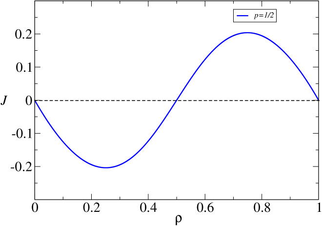
Figure 1: Current as a function of density for $K=1.$ Density dependent current reversal for single species assisted hopping model obeying dynamics (49) with $p=\frac{1}{2}$- the current becomes zero at $\rho^{\ast}=\frac{1}{2}$(point of reversal) and then reverses its direction as density is further increased.

To summarize, for the given dynamics (49) with some fixed value of $p,$ if we start with a very small particle density $\rho_{1}\approx 0$ and increase the density gradually, at first the average current flows towards right(if $p>1$) starting from zero(or, towards left(if $p<1$)), reaches a maximum(or, minimum) value, then decreases(or, increases) continuously until at some particular value of density $\rho^{\ast}_{1}=\frac{1}{2}$- which we call to be the point of reversal- the current $\langle J\rangle$ becomes zero, after which if we increase the particle density, current starts flowing in the opposite direction namely towards left (or, towards right). This incident of change in the direction of particle current as we tune the density for a fixed dynamics, is known as density dependent current reversal and that particular value of density at which the current equals to zero just before changing its direction, is termed as the point of reversal. We can see in Fig. 1 that the particles following the dynamics (49) with $p=\frac{1}{2},$ undergo a reversal in the direction of current with $\rho^{\ast}_{1}=\frac{1}{2}$.

IV.2 Negative differential mobility in AEM with $K=1$

In this section, we consider yet another specific case, where $p=1,q=e^{-\epsilon}$

$$010\mathop{\rightleftharpoons}_{e^{-\epsilon}}^{1}001~{}~{}~{}~{}~{}~{}~{}~{}~{}~{}110\mathop{\rightleftharpoons}_{e^{-\epsilon}\gamma^{-1}}^{\gamma}101~{}~{};\gamma=\frac{1}{1+\epsilon/2}$$ (53)

The above hop rates, when compared to Eq. (44) along with (45), imply that dynamics (53) lead to a pair factorized steady state with $g(1,0)=g(0,1)=e^{\epsilon/2}$,$g(0,0)=e^{\epsilon}$ and $g(1,1)=(1+\epsilon/2)$. Note that, in absence of the additional factor $\epsilon/2$ in (53) the isolated particles and crowded particles hop with same rates and the model no longer remains an assisted one. As usual, we define the net bias on the particles towards some direction, say right, as the logarithm of the ratio of the right hop rate to the left one. More elaborately, the bias on the isolated particles is $\mathrm{ln}(\frac{1}{e^{-\epsilon}})$ i.e. simply $\epsilon$ whereas the crowded particle feels a rightward bias given by $(\epsilon-2\mathrm{ln}(1+\epsilon/2)).$ Since, both the bias are monotonically increasing functions of $\epsilon,$ from here on, we simply consider $\epsilon$ as the bias and will discuss the behavior of the particle current for (53) as we change the bias $\epsilon$ for a given particle density. Firstly, from Eq. (47), we calculate the average current $\langle J\rangle$ for the present dynamics (53),

$$\langle J\rangle=\frac{1}{\lambda^{2}}\left[z_{1}(\rho_{0}e^{\epsilon}-\rho_{1}(1+\epsilon/2))+(z_{1}-1)\sqrt{\rho_{0}\rho_{1}z_{1}e^{\epsilon}}\right]$$ (54)

where $\lambda=\frac{1}{2}\left(e^{\epsilon}+z_{1}(1+\epsilon/2)+\sqrt{(e^{\epsilon}-z_{1}(1+\epsilon/2))^{2}+4z_{1}e^{\epsilon}}\right)$ and from the density-fugacity relation, one can also express the fugacity $z_{1}$ in terms of the densities and other parameters as follows

$$z_{1}=\frac{e^{\epsilon}}{(1+\epsilon/2)}+\frac{(1-2\rho_{0})}{2(1+\epsilon/2)^{2}\rho_{0}(1-\rho_{0})}\times$$ (55)

$$\left[e^{\epsilon}(1-2\rho_{0})+\sqrt{e^{\epsilon}(e^{\epsilon}(1-2\rho_{0})^{2}+4e^{\epsilon}(1+\epsilon/2)\rho_{0}(1-\rho_{0}))}\right].$$ (56)

Let us be more specific and analyze the system at density $\rho_{1}=\frac{1}{2}=\rho_{0}.$ Then the fugacity $z_{1}$ in the above equation simply relates to the bias $\epsilon$ as

$$z_{1}=\frac{e^{\epsilon}}{(1+\epsilon/2)}.$$ (57)

Correspondingly, substituting this value of $z_{1}$ in Eq. (54), the particle current at $\rho_{1}=\frac{1}{2}=\rho_{0}$ becomes

$$\langle J\rangle=\frac{1-e^{-\epsilon}(1+\frac{\epsilon}{2})}{2(1+\frac{\epsilon}{2}+\sqrt{1+\frac{\epsilon}{2}})}$$ (58)

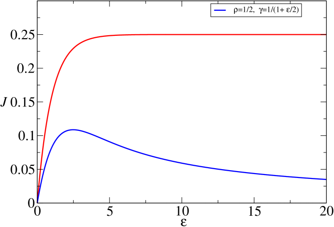
Figure 2: Negative differential mobility exhibited by particles of the single species assisted hopping model when the dynamics (44) takes the specified form of (53) in contrast to another specific case of (44) where $\gamma=1$ - both the systems are studied at particle density $\rho_{1}=\frac{1}{2}$.

If we plot the current($\langle J\rangle$) in Eq. (58) as a function of the bias($\epsilon$), as shown in Fig. 2. by the green curve, we observe that the current is zero at $\epsilon=0$ (as expected from dynamics (53) since $\epsilon=0$ leads to the equilibrium situation), then as we increase the bias the current increases. But at a finite value $\epsilon=\epsilon^{\star}\approxeq 2.4,$ $\langle J\rangle$ reaches to its maximum value, after which, as we increase the bias the current decreases gradually giving rise to negative differential mobility (i.e. $\frac{\mathrm{d}\langle J\rangle}{\mathrm{d}\epsilon}<0$ in the parameter region $\epsilon^{\star}<\epsilon<\infty$). This incidence of negative response is evident from the expression (58) because the current approaches to zero in both the limit $\epsilon\rightarrow 0$ and $\epsilon\rightarrow\infty$, so in between $0<\epsilon<\infty,$ there must be finite $\epsilon=\epsilon^{\star}$ at which the current reaches to an extremum and in one of the regions(either greater than or less than $\epsilon^{\star}$), the current as a result exhibits negative differential mobility. To emphasize the role of the factor $\epsilon/2,$ we present another curve (the red one) in Fig. 2 that corresponds to the current in absence of the factor $\frac{\epsilon}{2}$ in (53), more accurately, it corresponds to the dynamics (44) with $p=1,q=e^{-\epsilon},\gamma=1$. It is quite straightforward to prove that this particular dynamics results in a factorized steady state and the current there is simply $\langle J\rangle=(1-e^{-\epsilon})\rho(1-\rho)$. So, the response for $\rho_{1}=1/2=\rho_{0}$ in this case is just $\frac{\mathrm{d}\langle J\rangle}{\mathrm{d}\epsilon}=\frac{e^{-\epsilon}}{4}$ which remains positive always irrespective of the value of $\epsilon$- this ensures that in absence of the additional factor $\epsilon/2$ the dynamics (53) does not give rise to negative differential response and the corresponding steady state current only increases with increasing bias and ultimately, for large values of $\epsilon$, more precisely in the limit $\epsilon\rightarrow\infty,$ settles to a finite constant value $\rho(1-\rho)=\frac{1}{4}$.

Let us discuss qualitatively the difference between the situations with $\gamma=1$(red curve in Fig. that does not show negative differential mobility) in comparison to the case where $\gamma=1/(1+\epsilon/2)$(blue curve in Fig. exhibiting negative differential response in the regime $<\epsilon<\infty$) in dynamics (44). Actually in both the cases, the isolated particles hop with same rates but the crowded particles (meaning when particle hopping is assisted by neighboring particles, $110\rightleftharpoons 101$) differ. A part of this dynamics where the the immediate neighbour (of the of the three sites under consideration) is vacant, is

$$1100\mathop{\rightleftharpoons}_{e^{-\epsilon}\gamma^{-1}}^{\gamma}1010.$$ (59)

So when a crowded particle moves to right, it creates isolated particles(1’s) and destroys 11-pairs causing de-clustering or breaking of cluster of particles(1’s) creating more activity- whereas the corresponding left move decreases the number of isolated particles and increases number of 11-pairs i.e. the left move causes clustering of particles(1’s) implying decrease in activity. It is evident from Eq. (59) that due to the presence of the additional factor $\epsilon/2$ in the later case, as we increase $\epsilon,$ for large drive, the clustering of 1-s through the leftward move increase significantly for the dynamics corresponding to $\gamma=1/(1+\epsilon/2)$ in comparison to the case $\gamma=1$. Clusterization of 1’s with increasing bias in turn implies decrease in activity which results in decrease of particle current as $\epsilon$ increases. Consequently we have negative differential mobility of particles for the dynamics (53).

This concludes our discussion about the single species assisted hopping model with a generic dynamics of the form (54)- which possess pair factorized steady state when the rates are specified by the condition (45). We have shown explicitly that this model, with some specific choice of rates, as given by Eq. (49) and (53) can exhibit density dependent current reversal(Fig. 1) and negative differential mobility(Fig. 2) respectively.

V Assisted exchange model with $K=2$

In this section we will we describe one example of the dynamics Eq. for $K=2.$ We start by considering a specific rate function,

$$g(0,0) = \frac{3}{10},g(0,1)=\frac{1}{5},g(0,2)=\frac{2}{5},g(1,0)=\frac{1}{2},$$ (60)

$$g(1,1) = \frac{1}{2},g(1,2)=1,g(2,0)=\frac{1}{10},g(2,1)=\frac{1}{8},g(2,2)=\frac{1}{10}.$$ (61)

For exchange rates can be constructed from the pair weight function $g(.,.)$ in a straightforward way, using Eq. (8). The fugacities $z_{1}$ and $z_{2}$ corresponding to the particles of the two different species, can now be expressed as a function of the corresponding particle densities $\rho_{1},\rho_{2}$ as(using Eq. (43)),

$$z_{1}(\rho_{1},\rho_{2})=\frac{2\rho_{1}}{\rho_{0}(1-\rho_{0})^{2}}\left[(1-2\rho_{0})^{2}+3\rho_{0}(1-\rho_{0})+(1-2\rho_{0})\sqrt{(1-2\rho_{0})^{2}+6\rho_{0}(1-\rho_{0})}\right]$$ (62)

$$z_{2}(\rho_{1},\rho_{2})=\frac{\rho_{2}}{2\rho_{0}(1-\rho_{0})^{2}}\left[(1-2\rho_{0})^{2}+3\rho_{0}(1-\rho_{0})+(1-2\rho_{0})\sqrt{(1-2\rho_{0})^{2}+6\rho_{0}(1-\rho_{0})}\right]~{}~{}~{}~{}~{}$$ (63)

and the particle current, as given by (40), takes the following form

$$\langle J\rangle(\rho_{1},\rho_{2})=\frac{1}{\lambda^{2}}\left[\left(\frac{3}{10}\rho_{0}+\sqrt{\rho_{0}}s_{2}\right)(z_{1}+z_{2})-(\sqrt{\rho_{0}}+5s_{2})s_{2}\right]$$ (64)

$$\mathrm{where}~{}~{}~{}s_{2}=\left(\frac{\rho_{1}}{\sqrt{5}}+\frac{\rho_{2}}{5\sqrt{2}}\right)\frac{\left[(1-2\rho_{0})^{2}+3\rho_{0}(1-\rho_{0})+(1-2\rho_{0})\sqrt{(1-2\rho_{0})^{2}+6\rho_{0}(1-\rho_{0})}\right]}{\rho_{0}(1-\rho_{0})^{2}},~{}~{}~{}~{}~{}$$ (65)

with $\rho_{0}=1-\rho_{1}-\rho_{2}$. Finally, by replacing $z_{1,2}$ from (63) into (65)-one gets the expression of $\langle J\rangle_{I}(\rho_{1},\rho_{2})$ which is now only a function of the particle densities $\rho_{1,2}$ for the given set of values of the rates.

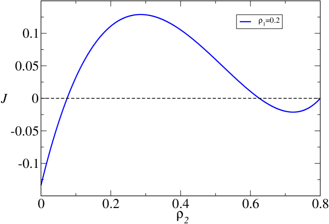
Figure 3: Density dependent current reversal for a two species assisted hopping and exchange process- multiple(two) point of reversal at $\rho_{1}=0.2$.

We have plotted this exact expression of the steady state particle current as a function of the second species particle density $\rho_{2}$ for a fixed value $\rho_{1}=0.2$- the resulting curve is shown in Fig. (3). We see that in Fig. (3), the current reverses its direction twice in contrast to the case $k=1$ in Fig. (1) where the current changed its direction only once giving rise to a single point of reversal, here in Fig. (3), clearly twice change in the direction of current results in multiple points of current reversal which in this case are $\rho_{2}^{\ast}\approx 0.07$ and $\rho_{2}^{\ast}\approx 0.62$ where the current become zero before reversing its direction. Along with this event of multiple reversal points, note that the current in Fig. (3) is still nonzero at $\rho_{2}=0$ because there is a finite number of particles of the first species still hopping on the lattice whereas for the $K=1$ case in Fig. (1) the current was naturally zero at $\rho_{1}=0$. Also note that this current reversal could also be observed by tuning $\rho_{1}$ with a fixed value of $\rho_{2}$. In fact, in general, if one plots $\langle J\rangle(\rho_{1},\rho_{2})$ as a function of both $\rho_{1}$ and $\rho_{2}$, we may expect a line of reversal in the $\rho_{1}-\rho_{2}$ plane along which the current becomes zero before changing its direction.

So, like single species assisted hopping model, we have shown that the emergence of density dependent current reversal can also occur for two species assisted hopping and exchange process- this leads us to believe that current reversal can generally happen in multi- species assisted hopping and exchange models for a broad class of rates.

V.1 Negative differential mobility in AEM with $K=2$

Just like current reversal, in this section, we would like to show that assisted exchange models exhibits negative differential mobility of particle current. In particular, we consider $K=2$ with pair-weight functions-

$$g(0,0)=e^{\epsilon},g(1,0)=g(0,1)=e^{\epsilon/2},g(1,1)=(1+\frac{\epsilon}{2}),g(2,0)=e^{\epsilon/5},g(0,2)=e^{7\epsilon/10},$$ (66)

$$g(1,2)=(1+\frac{\epsilon}{2})e^{\epsilon/5},g(2,1)=(1+\frac{\epsilon}{2})e^{-3\epsilon/10},g(2,2)=(1+\frac{\epsilon}{2})e^{-\epsilon/10}.$$ (67)

Corresponding two species assisted exchange dynamics can be derrived from Eq. (8). Since, here we focus on the current as a function of the bias $\epsilon,$ we consider the particle densities of the two species to be fixed at $\rho_{1}=0.6$ and $\rho_{2}=0.1$ respectively. It is quite straightforward to check that all the relevant biases in the total particle current are increasing functions of the bias $\epsilon$ under consideration. Now, the exact form of the current in this case can be calculated directly from Eq. (29)- but it looks very complicated-so we omit the functional form here. Instead, we show the plot of the total particle current as a function of the bias in Fig. (4).

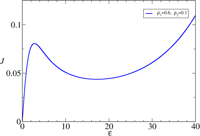
Figure 4: Negative differential mobility exhibited by the total particle current in the region $3\lessapprox\epsilon\lessapprox 17$ for a two species assisted hopping and exchange model at densities $\rho_{1}=0.6,\rho_{2}=0.1$

In Fig. (4), we observe that in the region as we increase the bias, the current decreases indicating the onset of negative differential mobility of the particles. Note the difference in the qualitative features of the negative response for the single species problem in Fig. (2)(green curve) with respect to the negative mobility showed by the two species model in Fig. (4)- in the later case, the negative response occurs in a bounded region value of the bias, more precisely for $3\lessapprox\epsilon\lessapprox 17$ i.e. the current, which at first increases with bias before decreasing in a certain bias value region, can increase again with bias beyond that region whereas in Fig. (2) once the current starts decreasing with increasing bias-it never goes up again resulting in no upper bound in region of bias causing negative response which is $4\lessapprox\epsilon<\infty$.

.

VI Conclusion

We have introduced an assisted hopping and exchange model on a one dimensional periodic lattice with hard core particles of $k$ (any finite positive integer) different species along with vacancies- the dynamics conserves the total number of particles as well as the number of particles of each species. The model is called assisted because the hop rate of any kind of particle to a vacant nearest neighbor or the exchange rate between two different kind of particles- both explicitly depend on the presence of the particle type or vacancy in the neighboring sites other than the sites involved in the hopping or exchange process. For example, we considered a single species assisted hopping model(obviously there is no exchange here) where the isolated particles(having both neighbors vacant) and crowded particles(having one neighbor vacant) move with different rates. Firstly, we investigate the possible steady state measure of this stochastic process and obtained that a pair-factorized steady state is indeed possible for two very different broad class of dynamics. Since the pair factorized state generates spatial correlation by definition, we opt for a transfer matrix formalism that helps us to calculate the spatial correlation function and expectation values of several other observables. We are mostly interested in the particle current that characterizes a non-equilibrium state- so we have derived exact expressions for the current in the corresponding PFSS of both the dynamics. To illustrate intriguing features like density dependent current reversal for a fixed set of rates and negative differential response of the particle current with increasing bias, we have extensively discussed a single species assisted hopping model(where isolated and crowded particles hop with different rates) that resembles to partially asymmetric conserved lattice gas asep_9 . Moreover, these interesting events of current reversal and negative differential mobility has also been described briefly for two species assisted hopping and exchange model with specified rates, where we observe additional features like multiple points of reversal in context of current reversal and an unusual response in particle current where current as a function of bias shows two extrema.

We conclude that the phenomena like density dependent reversal of current and negative differential mobility of particles can generally occur in multi-species assisted hopping and exchange models for suitable choice of the dynamical rates. One can in general ask if AEM can have a steady state measure, other than PFSS and explore the possibility of phase separated states. It would be interesting to explore these exactly solvable models to study the characterization of non-equilibrium states in terms of current and its higher order cumulants.

References

- (1) Nonequilibrium Statistical Mechanics In One Dimension, ed. V. Privman, 1997 Cambridge University Press, Cambridge.
- (2) B. Derrida and J. L. Lebowitz, Phys. Rev. Lett. 80, 209 (1998).
- (3) A. Gerschenfeld and B. Derrida, EPL 96, 20001 (2011).
- (4) E. Akkermans, T. Bodineau, B. Derrida and O. Shpielberg, EPL 103, 20001 (2013).
- (5) A K. Chatterjee and P. K. Mohanty, J. Stat. Mech., 2017 093201 (2017).
- (6) R. K. P. Zia, E. L. Præstgaard, and O.G. Mouritsen,Am. J. Phys. 70, 384 (2002).
- (7) A. S. Maksimenko and G. Ya. Slepyan, Phys. Rev. Lett. 84, 362 (2000).
- (8) P. Baerts, U. Basu, C. Maes, S. Safaverdi, Phys. Rev. E 88, 052109 (2013).
- (9) A. K. Chatterjee, U. Basu and P. K. Mohanty, Phys. Rev. E 97, 052137(2018).
- (10) R. Eichhorn, P. Reimann, and P. Hänggi, Phys. Rev. Lett. 88, 190601 (2002). ibid, ̵̈Phys. Rev. E 66, 066132 (2002).
- (11) A. Ros, R. Eichhorn, J. Regtmeier, T. T. Duong, P. Reimann and D. Anselmetti, Nature 436 928 (2005).
- (12) J. Cividini, D. Mukamel, and H. A. Posch, J. Phys. A: Math. Theor. 51, 085001 (2018).
- (13) J. Marro, R. Dickman, Nonequilibrium Phase Transitions in Lattice Models, 1999 Cambridge University Press, New York.
- (14) B. Schmittmann and R. K. P. Zia, Statistical Mechanics of Driven Diffusive Systems, ed. C. Domb and J. L. Lebowitz, 1995 Academic Press, New York.
- (15) G. M. Schütz, Phase Transitions and Critical Phenomena Vol. 19, ed. C. Domb and J. L. Lebowitz 2000 Academic Press, London.
- (16) B. Derrida, E. Domany and D. Mukamel, J. Stat. Phys. 69, 667 (1992).
- (17) S. Prolhac and K. Mallick, J. Phys. A: Math. Theor. 41(17), 175002 (2008).
- (18) T. M. Liggett, Stochastic Interacting Systems: Voter, Contact and Exclusion Processes, 1999 Springer, New York.
- (19) S. Prolhac and K. Mallick, J. Phys. A: Math. Theor. 41(36), 365003 (2008).
- (20) M. Gorissen, A. Lazarescu, K. Mallick and C. Vanderzande, Phys. Rev. Lett. 109, 170601 (2012).
- (21) A. Lazarescu, J. Phys. A: Math. Theor. 46, 145003 (2013).
- (22) B. Derrida, J. Stat. Mech., P07023 (2007).
- (23) M.R. Evans, Europhys. Lett. 36, 13 (1996).
- (24) U. Basu and P. K. Mohanty, Phys. Rev. E 79, 041143 (2009).
- (25) A. P. Isaev, P. N. Pyatov and V Rittenberg, Phys. A: Math. Gen. 34, 5815 (2001)
- (26) M. R. Evans, T. Hanney, J. Phys. A: Math. Gen. 38, R195(2005).
- (27) M. Clincy, B. Derrida, and M. R. Evans, Phys. Rev. E 67, 066115 (2003).
- (28) A. Ayyer, E. A. Carlen, J. L. Lebowitz,P. K. Mohanty, D. Mukamel and E. R. Speer, J. Stat. Phys 137, 1166 (2009).
- (29) P.F. Arndt, T. Heinzel, and V. Rittenberg, J. Phys A: Math. Gen. 31, L45 (1998); ibid, J. Stat. Phys. 97, 1 (1999).
- (30) R. A. Blythe, M. R. Evans, J. Phys. A: Math. Theor. 40, R333 (2007).
- (31) Y. Kafri, E. Levine, D. Mukamel, G.M. Sch ̵̈ütz, and J. Török, Phys. Rev. Lett. 89, 035702 (2002); M. R. Evans, E. Levine, P. K. Mohanty, D. Mukamel, Euro. Phys. J. B 41, 223 (2004).
- (32) A. Kundu and P. K. Mohanty, Physica A 390, 1585 (2011).